Local Buckling Behavior and Plastic Deformation Capacity of High-Strength Pipe at Strike-Slip Fault Crossing
by
 ,
,
Xiaoben Liu
1,2 ,
,
Hong Zhang
1,*,
Baodong Wang
1,
Mengying Xia
1,2,*,
Kai Wu
1,
Qian Zheng
1 and
Yinshan Han
1 1
College of Mechanical and Transportation Engineering, China University of Petroleum-Beijing, Beijing 102249, China
2
Department of Civil and Environmental Engineering, University of Alberta, Edmonton, AB T6G 2W2, Canada
*
Authors to whom correspondence should be addressed.
Metals 2018, 8(1), 22; https://doi.org/10.3390/met8010022
Submission received: 17 November 2017
/
Revised: 26 December 2017
/
Accepted: 26 December 2017
/
Published: 31 December 2017
(This article belongs to the Special Issue Mechanical Behavior of High-Strength Low-Alloy Steels)
Abstract
:As a typical hazard threat for buried pipelines, an active fault can induce large plastic deformation in a pipe, leading to rupture failure. The mechanical behavior of high-strength X80 pipeline subjected to strike-slip fault displacements was investigated in detail in the presented study with parametric analysis performed by the finite element model, which simulates pipe and soil constraints on pipe by shell and nonlinear spring elements respectively. Accuracy of the numerical model was validated by previous full-scale experimental results. Insight of local buckling response of high-strength pipe under compressive strike-slip fault was revealed. Effects of the pipe-fault intersection angle, pipe operation pressure, pipe wall thickness, soil parameters and pipe buried depth on critical section axial force in buckled area, critical fault displacement, critical compressive strain and post buckling response were elucidated comprehensively. In addition, feasibility of some common buckling failure criteria (i.e., the CSA Z662 model proposed by Canadian Standard association, the UOA model proposed by University of Alberta and the CRES-GB50470 model proposed by Center of Reliable Energy System) was discussed by comparing with numerical results. This study can be referenced for performance-based design and assessment of buried high-strength pipe in geo-hazard areas.
1. Introduction
Buried steel pipelines serve as the main means of transportation of both raw and processed hydrocarbon fluids worldwide. High-strength line pipe steels are preferred by operators for their higher profit induced by the increased throughput of the products [1]. The large expanse of pipe routine makes crossing some geo-hazard areas inevitable, such as active seismic faults. Large ground-relative displacements along the fault trace will cause axial compression (or tension) and lateral bending in pipe, which may be large enough to initiate local buckling or tensile fracture failure [2]. As crucial lifelines, the integrity of steel pipelines at tectonic fault crossings has been paid close attention to by both academic and industrial spheres.
Newmark and Hall conducted the pioneer work for analytical strain analysis of pipe at fault crossing [3], in which the pipe was assumed to deform like a cable. Due to its high simplicity, the Newmark method is still widely used in industry for the primary design of a pipe subjected to fault movement. Thereafter, a series of analytical or semi-analytical models were developed for refined analysis of pipe strain or stress under fault displacement. Kennedy et al. [4] and Wang et al. [5] considered pipe bending with assumptions that pipes deform as curved arcs and elastic beams. In more recent decades, more complicated semi-analytical approaches were proposed by Karamitros et al. [6], Trifonov et al. [7], and Zhang et al. [8], who considered the elastoplastic characteristic of pipe steel’s constitutive model and their effects on pipe’s nonlinear stress distributions in sections of large deformed pipe segments near fault trace. Although these analytical methods can be more easily popularized in guidelines for engineering applications, they also have severe weaknesses. Even the latest analytical methods are still based on the beam assumption of pipe, which is incapable of describing the local deformation of pipes subjected to compression or combined with bending loads.
For pipes subjected to compression at strike-slip fault crossings, numerical and experimental models were mostly utilized for pipe performance analysis. Due to the restrictions of hydraulic loading facilities, experimental investigations were all focusing on low- to medium-strength steel pipes or high-density polyethylene (HDPE) pipes with similar nonlinear stress-strain response as steels. Ha et al. [9,10] and O’Rourke et al. [11,12] conducted centrifuge and full-scale tests of buried HDPE under compression strike-slip faults. Results show that these two methods derived similar pipe response with the similar parameters. Jalali et al. [13,14,15] performed a full-scale experiment on responses of both American Petroleum Institute (API) Grade-B steel and HDPE pipes under reverse fault displacements. Both global and local buckling behavior were captured in his investigation. Valuable conclusions on pipe soil interactions were also obtained in their experiments.
Based on the experimental results, a lot of calibrated numerical models were developed for further investigations on pipe performance subjected to compression strike-slip fault movements. Generally, numerical models can be classified by the simulation methods for pipe and soil constraint on pipe. Pipes can be simulated by pipe (elbow) elements or shell elements. Pipe (elbow) elements have the advantage in calculation efficiency, but they are incapable of demonstrating the pipe wall folding phenomenon in pipe, when local buckling occurs. Soil constraints on pipe can be modeled by discrete nonlinear soil spring elements or the surface-to-surface contact between the shell elements simulating pipe and the continuum solid elements simulating surrounded soil [16]. Adopting the numerical models, stress and strain behaviors of different kind buried pipes under various types of active faults have been studied. Using finite element (FE) models with pipe (elbow) elements and nonlinear spring elements, Xie et al. validated the numerical models by comparing them with centrifuge experiment results [17,18]. Joshi et al. conducted parametric analysis on beam buckling behavior of steel pipe at reverse fault crossing [19]. Uckan et al. proposed a simplified model to derive the response of curved pipeline at strike-slip fault crossing [20]. Liu et al. developed a prediction model on peak pipe compressive strain based on the numerical results and nonlinear regression method [21]. Melissianos et al. conducted performance assessment of buried pipe at fault crossing [22,23]. Using Finite Element (FE) models with shell elements and nonlinear spring elements, Karamitros et al. validated his analytical model [6]. Liu et al. proposed a semi-empirical equation for strain demand of pipeline at oblique-reverse fault crossing [24]. Xu et al. investigated the wrinkling phenomenon under reverse fault [25]. More recently, using FE models with shell elements and continuum solid soil elements, Kaya et al., simulated the failure behavior of a welded steel pipe at Kullar fault crossing [26]. Zhang et al. discussed the collapse behavior of pipeline buried in rock under strike-slip fault movement and reverse fault displacements [27,28]. Vazouras conducted series of numerical models to investigate the failure behavior of pipeline under strike-slip fault movement in detail [29,30,31,32]. Trifonv et al. also built a rigorous numerical model to analyze the influence of the trench on the pipeline performance at fault crossing [7].
However, although extensive research is available, relatively little literature exists on the topic of high-strength pipe buckling behavior specifically. Some attempts were made by Liu et al. to investigate the effects of yield strength and strain hardening parameter on the local failure behavior of high-strength pipes subjected to reverse faulting [33]. Kainat et al. investigated the influences of geometric imperfections on high strength pipe’s buckling behaviors [34]. Neupane et al. captured the anisotropic characteristic of high-strength pipe steel in longitudinal and circumferential directions, and discussed its effects on buckling response of pipe induced by frost heave in northern areas [35,36]. However, comprehensive investigations on local buckling of high-strength pipes in various engineering cases are urgently needed. Thus, a systematic analysis was conducted in this paper on the local buckling behavior of high-strength of X80 steel pipeline subjected to strike-slip fault displacements. Mechanical response of X80 pipe at onset moment when local buckling occurs was studied. Influences of the pipe-fault intersection angle, pipe diameter, pipe wall thickness, pipe operation pressure, soil parameters, pipe buried depth on pipe’s buckling behavior were all investigated in detail. Based on the finite element results, applicability of some well-recognized compressive strain criteria on local buckling failure recognition for high-strength pipe was evaluated in a wide range of common parameters.
2. State of the Art in Buckling Failure Criteria for Line Pipes
Compressive local buckling is a limit state for pipeline under compressive load. In strain-based design, the principle purpose is to keep the strain demand (i.e., the maximum longitudinal compressive strain in pipe) in pipe less than the compressive strain capacity of pipe (i.e., the longitudinal pipe strain at the onset moment of pipe buckling) [1]. Thus, to provide suitable references for pipeline designers and operators, a series of prediction models for compressive strain capacity have been established and adopted by different guidelines and standards. In this section, three well-recognized models for compressive strain capacity of plain pipe are presented briefly.
2.1. CSA Z662 Model (2015)
The CSA Z662 model [37] was initially based on Gresnigt’s research in 1980s [38]. Its latest version was released in 2015. Some modifications have been made to Gresnigt’s model to improve the model’s accuracy for pipes with high internal pressure. This model is the one most widely used so far. A lot of codes and standards directly adopt this model to calculate the compressive strain capacity of steel pipes , such as the guideline for design of buried steel pipeline [39], and the aseismic guidelines for pipes in India [40]. The model considers the effects of pipe diameter to wall thickness ratio D/t and operation pressure P on pipe’s strain capacity directly. It should be noted that the CSA formula was derived by regression of lower-bound test data. Thus, material property parameters and pipe geometrical imperfections were also implicitly considered. The CSA formula is given by Equation (1).
where D is the pipe diameter, t is pipe wall thickness, D/t ≤ 120, P is the pipe operation pressure, σy is the yield strength of pipe steel.
2.2. UOA Model (2006)
The UOA models [41] were developed by structure group at the University of Alberta in 2006 [41]. The equations were established throughout regression analysis on a large number of finite element models and full-scale experimental results. The considered steel grades in parametric analysis included X52, X65 and X80. Four groups of CSA Z662 equations were finally obtained for plain pipes with yield plateau type or round house type stress-strain curve and girth weld pipe with yield plateau type or round house type stress-strain curve. For in the numerical analysis of presented paper, the pipe was considered as a plain pipe with roundhouse-type stress-strain curve; the equation for this kind of pipes was listed here (Equation (2)).
where hg is the height of the geometry imperfection which is defined as the peak-to-valley height of the surface undulation, 50 ≤ D/t ≤ 90.
2.3. CRES-GB 50470 Model (2017)
The CRES model [42] was established by the Center for Reliable Energy Systems in 2013 under the support of the US Department of Transportation [42]. Similar to the UOA model, it is developed based on a large amount of finite element models. This model has been recently recommended by the latest version of China’s national standard for seismic design and assessment of oil and gas transmission pipelines (GB 50470) [43]. The influence factors considered in the CRES-GB 50470 model is the most comprehensive one in reported research so far, including ratio of pipe diameter to pipe wall thickness D/t, operation pressure, ratio of yield strength to tensile strength of pipe material σy/σu, geometry imperfection hg, girth weld, Lüder’s strain, and net-section stress σa. For plain pipes with roundhouse-type stress-strain curves, the CRES equation is as follows:
where σa is the applied net-section stress in the longitudinal direction of pipe, which can be derived from the stress demand analysis. If σa is not available, σa = 0; 20 ≤ D/t ≤ 104, 0.76 ≤ σy/σu ≤ 0.96.
Applicability of these models for high-strength steel pipe will be further evaluated by the numerical results of the buried X80 pipeline under compression strike-slip fault in subsequent sections. It should be noticed that some formulas focusing on compressive strain capacity of offshore pipes with small diameter to wall thickness ratio were recommended by the API-1111-1999 [44], DNV OS F101 [45]. For their incapable application to common onshore high-strength pipelines with large diameter to wall thickness ratio, they are not discussed here.
3. Finite Element Model
3.1. Modelling Pipe-Soil Interaction with Discrete Nonlinear Soil Springs
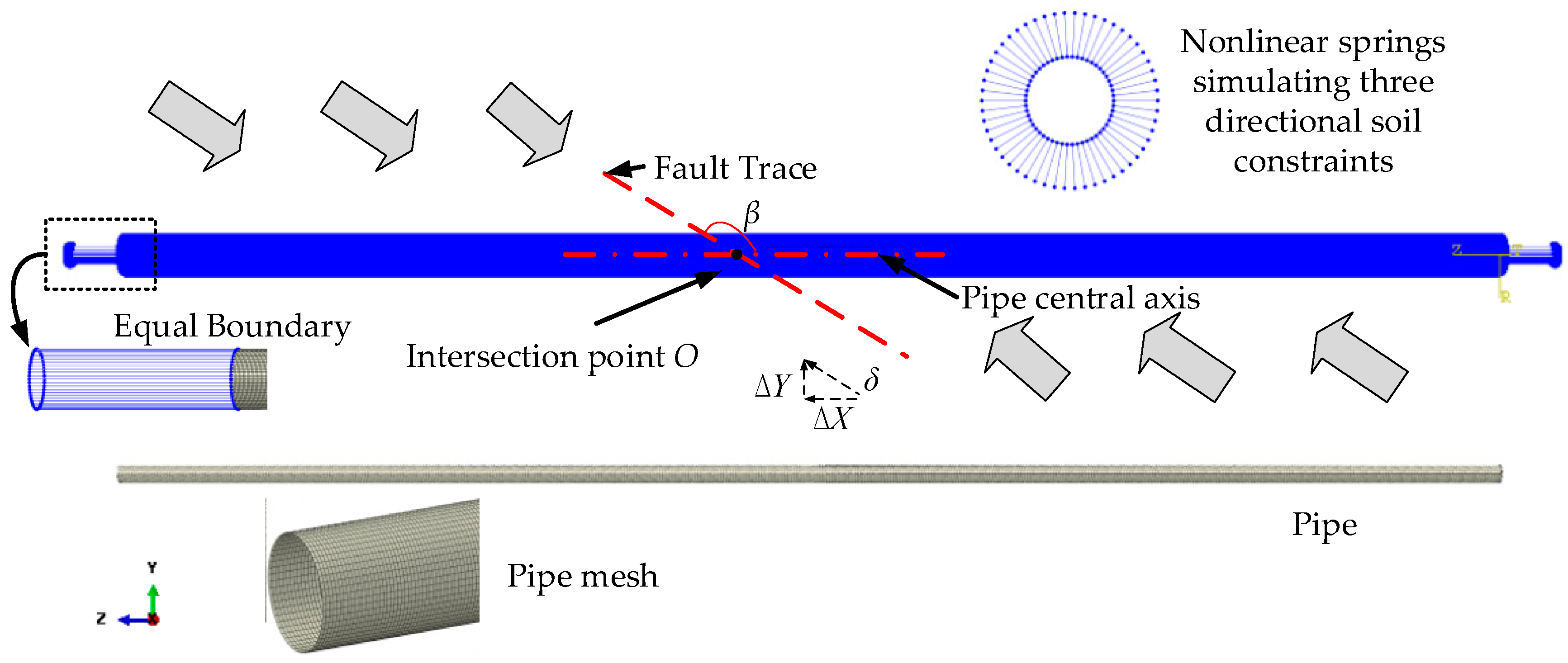
For buried steel pipelines, constraints will be induced on them by the surrounding soil in the axial, horizontal and vertical directions, if they have relative motions. The soil-applied force on pipe or pile structures is commonly nonlinear, which can be described by the p-y curves derived by geotechnical researchers [12]. There is a lot of available literature on this topic, among which the design recommendations specified by the ASCE Guideline [46] and ASCE-ALA Guideline [39] is the most widely used one for design and assessment of buried pipelines. According to the ASCE-ALA Guideline, soil constraints on pipe can be modeled using nonlinear soil springs with elastic plastic constitutive properties in three perpendicular directions, i.e., the axial, lateral and vertical directions of pipe central axis as illustrated in Figure 1, where continuous lines represent the real characteristic and dashed lines represent the approximation implemented in the model. The parameters Pu, Tu, and Qu(Qd) represent the peak soil resistances per unit length of pipes, while ∆p, ∆t, and ∆qu (∆qd) represent the corresponding yield displacements in three directions (i.e., lateral, axial, and vertical), respectively. Values of all these parameters can be readily obtained according to the ASCE-ALA Guideline with soil property parameters derived from field investigation. For numerical modelling, most commercial finite element software has developed spring elements capable of coupling a force with relative displacement nonlinearly. In this paper, the 3D SPRING elements (SPRING2) in general FE package ABAQUS were utilized for numerical investigation [47].
3.2. Modelling of Pipe
In this study, pipe segments were all modeled by four node shell elements with reduced integration (S4R) in general FE software ABAQUS (Dassault Systèmes, version 6.14, Johnston, RI, USA). The Second West-to-East Gas Pipeline in China was taken as the prototype for this study. The modeled pipe in numerical model was set to be 100 m in total, 50 m each at both sides of the fault trace, with pipe nodes at the two axial ends connected with nonlinear springs (SPRING2) to model the axial constraint of longitudinally adjacent pipes on the 100 m long pipe at fault trace (Figure 2). A constitutive model of the equivalent spring will be described in the subsequent section (Section 3.3). A refined mesh was achieved by sensitivity analysis with 54 elements discretized in circumferential direction. In addition, setting the longitudinal length of all the shell elements to be 0.04 m was proven to be accurate for simulating the wrinkling behavior of pipe induced by local buckling [33].
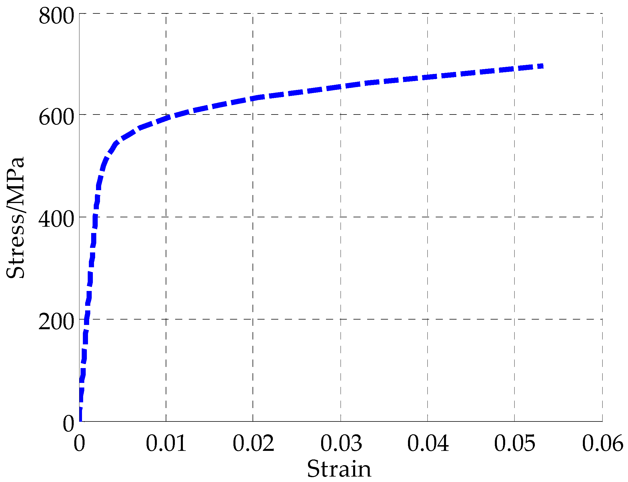
The material stress-strain model for X80 line pipeline considered in this study is plotted in Figure 3. A large-strain von Mises plasticity model with isotropic hardening is used for the steel in numerical investigation. The curve can also be expressed by the Ramberg-Osgood model (Equation (6)), with yield strength as 550 MPa, strain hardening exponent r as 17 and the yield offset parameter α as 0.94 [48].
The finite element model was calculated in two nonlinear static steps. In the first step, all soil nodes are fixed, and operation pressure was applied in the inner surface of the entire pipe. In the second step, all the soil nodes on the right of the fault trace were displaced with fault displacements both longitudinally and laterally in a horizontal plane, while all the soil nodes on the left of the fault trace were all kept motionless. As shown in Figure 2, the longitudinal displacement ∆X and the lateral displacement ∆Y are δcosβ and δsinβ, respectively. In order to insure the convergence of the iterative calculation of the FE model, nonlinear stabilization algorithm was utilized in the second step [49], the initial step size of the fault displacement load step is set to be 0.05, with the minimum allowable step size set to be 10−6. If there is no pressure in the pipe, the first step should be removed. It also should be mentioned that the proposed model can be suitable for dynamic simulations by replacing the static analysis step to explicit dynamic step. With the performed dynamic analysis, the model can be utilized to predict the transients associated with buckling phenomena, thus possibly allowing integration with the techniques adopted for leak detection [50,51,52,53].
3.3. Constitutive Model of Equivalent Boundary
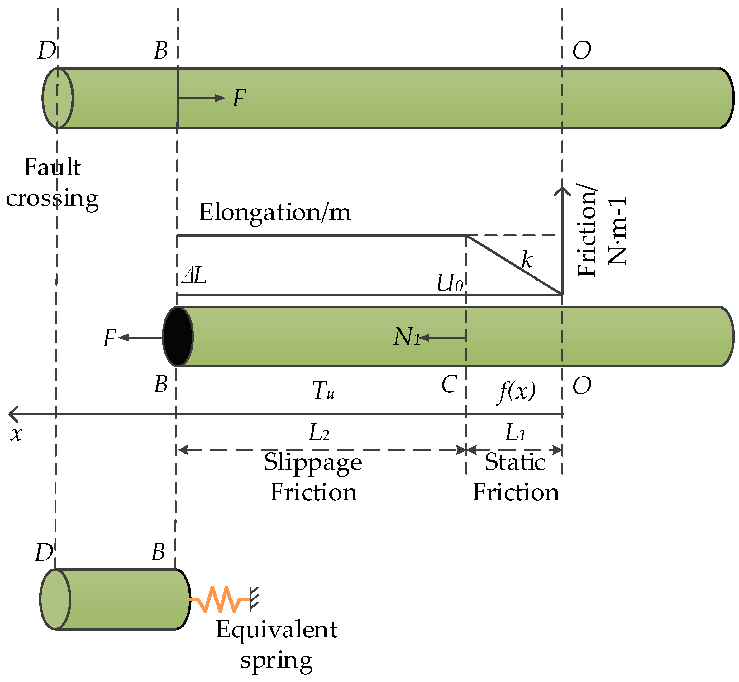
When buried pipelines are subjected to fault movement, relative displacements appear between the pipe and the surrounding soil. The equivalent boundary model was used to reduce the element numbers in numerical calculation by using few nonlinear springs simulating the axial constraints on pipe induced by the adjacent pipes, as show in Figure 4. Liu et al., developed the constitutive model of the equivalent boundary [54], which represents the relationship of the axial force F and the pipe extension at Point B ∆L (Equation (7)).
where E is the elastic modulus, A is the pipe cross section area, Tu is the slip friction force on unit length of pipe, i.e., the peak axial soil resistant force of soil spring, ∆t is the in the axial direction, σy is the yield strength of pipe material.
3.4. Validation of Proposed Model
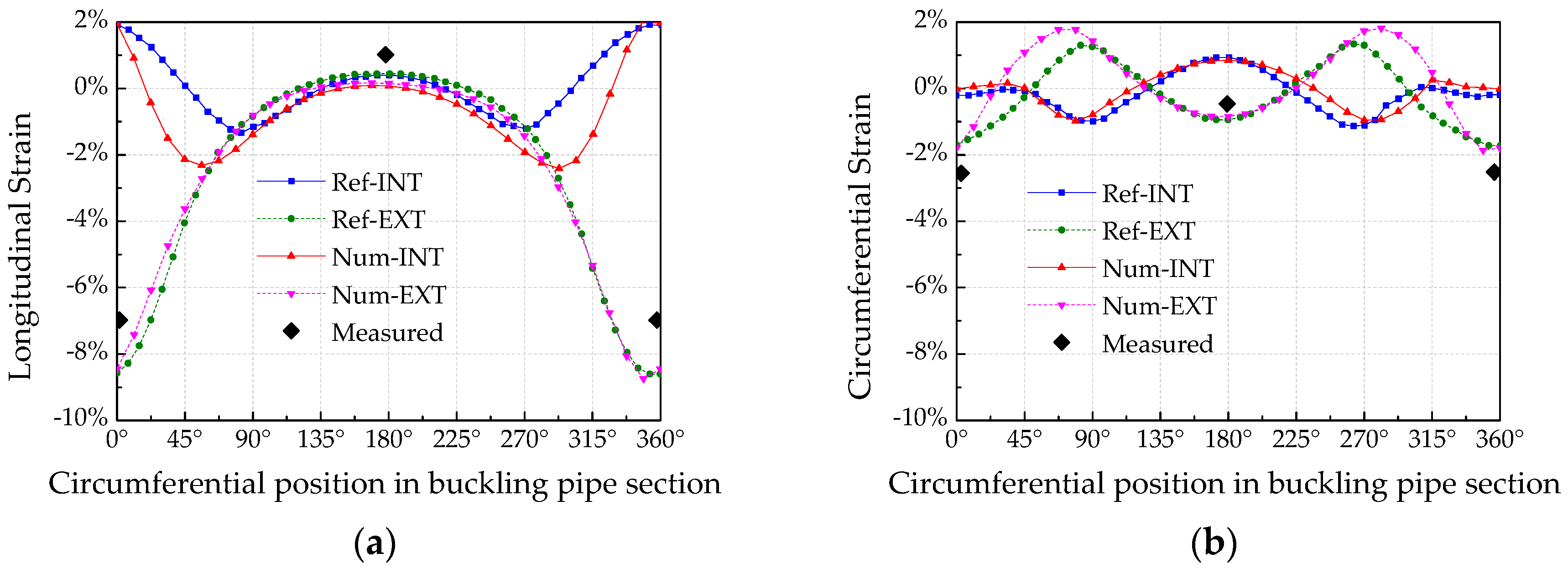
The full-scale experimental results for buried HDPE pipe subjected to strike-slip fault movements conducted by O’Rourke and a corresponding numerical model established by Xie et al. were used here to validate our established numerical model [11,18]. Material characteristics of HDPE material are similar with high-strength pipe strength, which has a roundhouse-type stress-strain curve but with a much smaller yield strength. The experimental pipe is a 10.56 m long pipe with 0.4 m diameter and 0.0024 m wall thickness, and the fault trace is located at the axial center of the pipe with a 65° intersection angle with the pipe axial axis. As the tested pipe is smaller than the steel pipes mentioned in Section 3.2, dimensions of the pipe was revised to be the same as the experiment pipe. The soil spring parameters in the validation model were also directly obtained from the experimental results. Furthermore, as the test PE pipe has smaller pipe diameter, the pipe was re-meshed into 48 elements in pipe’s circumferential direction, which is the same as Xie’s numerical model. The calculation process is the same as the one described in Section 3.2. Figure 5 shows comparison results of longitudinal and circumferential strains in the internal and external surfaces of the buckling section in the pipe under 0.61 m fault displacement. The results contain the proposed numerical results (Num-INT and Num EXT in Figure 5) and the numerical results derived by Xie et al. through a refined 3D finite element model (Xie-INT and Xie EXT in Figure 5) [18] and the measured results (measured in Figure 5).
It can be readily obtained that the maximum longitudinal compressive strain equals −8.5% numerically, locating at 0° position of the pipe section. While the maximum longitudinal tensile strain is less than 1%, located at the opposite direction of the pipe. The circumferential strain values are much smaller than the longitudinal ones. This is mainly induced by the local buckling, which itself is induced by axial compression of pipe. Generally, it can be found that strain results of the presented numerical model matches quite well with measured experimental results and the numerical results derived by Xie et al. [18].
4. Results and Discussion
4.1. Baseline Analysis for the Local Buckling Failure of X80 Pipe Steel
In the section, a baseline analysis was presented for plastic buckling phenomenon of X80 pipe subjected to a strike-slip fault with an intersection angle to be 150°. The pipe diameter and wall thickness are 1.219 and 0.0184 m, respectively. The operation pressure of pipe is 12 MPa. The pipe is buried in cohesive soil with buried depth of 2 m. The internal friction angle of soil is 33°.
As one limit state of pipe, local buckling decreased pipe bearing capacity both longitudinally and circumferentially. For numerical investigation, the section axial force in the buckled area can be monitored for identification of onset of local buckling of pipe (Liu et al. [33,49]). The section axial force in this study represents the local longitudinal internal force of pipe segments in the buckled area. When its value decreases with the increasing of applied fault displacement, the partial stiffness of pipe in this area starts decreasing representing the initiating of local buckling. Relationship of the section axial force with the axial membrane stress of the shell element is as follows:
where σaxial is the axial membrane stress of the shell element; SSectionS4R is the section area of the shell element. As the pipe was discretized into 54 elements circumferentially, SSectionS4R = πDt/54.
Figure 6 shows the relationships of section axial force in buckled area SF and peak axial compressive strain εaxial with fault displacement δ. If δ is relatively small, SF increases almost linearly with the δ. If δ > 0.2 m, gradient of SF decreases obviously until SF reaches its peak value, where it drops suddenly representing the local collapse behavior of pipe. The critical pipe section axial force in the buckled area SFcrit and the relative critical fault displacement δcrit are 5500 KN and 0.465 m, respectively. Compared with the trend of εaxial with δ, it can be found that before δ reaches δcrit, εaxial increases gradually with the increase of δ; once δ reaches δcrit, εaxial exhibits an abrupt increase. The critical axial compressive strain εcrit for the onset of local buckling can then be derived for the curve as −1.88%.
Figure 7 plots the contours of SF and εaxial in pipe with various fault displacements, as well as the detail distribution of εaxial in buckled area. Results show that, distribution of SF have almost no variations when δ increases from 0.182 m to the critical value 0.465 m. However, after that, a small increase of δ (δ = 0.468 m) induces wavy distribution of SF with small amplitude in buckled area. Immediately after this, an obvious bulging pattern occurs in the pipe as well as a much more severe wavy distribution of SF. Compared with the section axial force results, variations of axial strain in the buckled area during this process are more obvious. At the critical fault displacement, an obvious strain concentration appears in the buckled area. After that, during the post buckling stage, severe wavy distribution of axial strain occurs when δ = 0.468 m, which quickly concentrates to one wave in the center of the bucked area. Above all, results show that, when local buckling occurs, pipe loses its partial bearing capacity. The section axial force drops immediately after the onset of local buckling, with axial strain increasing abruptly induced by the large deformation.
4.2. Effects of Pipe-Fault Intersection Angle
When pipes crossing compression strike-slip faults with pipe-fault intersection angle larger than 90°, they are subjected to combined compression and bending load induced by the axial and lateral soil displacement components. With a large intersection angle (i.e., 175°), the pipe is subjected to severe axial compression and relatively small bending. While with a small intersection angle (i.e., 105°), the pipe is subjected to severe bending and relatively small axial compression.
In this section, five typical intersection angles, i.e., 105°, 120°, 135°, 150°, 175°, are considered to investigate their effects on critical fault displacement and critical axial compressive strain for local buckling, as shown in Figure 8. When δ is smaller than 0.45 m, trends of SF with δ are quite similar for the cases with different intersection angles. When δ reaches 0.4612 m, SF for the condition that β = 135° first drops, representing the local buckling of pipe.
Relationships between the critical fault displacements δcrit and pipe fault intersection angles β are also illustrated in Figure 9. It can be derived that for compression strike-slip fault, if β < 135° δcrit decreases with β, else δcrit increases with β. Thus, when pipe fault intersection angle equals 135°, the pipe is more likely to be buckled and fail. This is mainly because when pipe fault intersection angle equals 135°, the combined effect of bending induced by lateral fault displacement δscosβ and compression induced by the axial fault displacement δssinβ is the severest, which makes the pipe more likely to be buckled.
The critical axial compressive strain εaxial for the five cases were captured and compared with the commonly used failure criteria introduced in Section 2. It should be mentioned that as a perfect pipe was used in numerical models in this study, the height of the geometry imperfection was set to be 1%t, a minimum value recommended by CRES (Liu et al. [42]) to calculate the critical compressive strain values. As shown in Figure 10, the derived critical strain values are all near 2%, with a small variation when the intersection angle changes. While for all the three models in Section 2 only consider effects of the pipe geometry parameters and operation pressures on εaxial, their calculated critical strain results will keep the same for these cases with various intersection angles.
It can be further observed that for the three considered models, the CSA Z662 model results are mostly conservative, which is almost less than half of the results of the UOA model, CRES-GB 50470 model and FE model. The UOA model results are larger than derived FE model results, representing un-conservative prediction of pipe’s strain capacity in actual loading conditions, which may limit its application. As for the CRES-GB 50470 model, its results are a little conservative and in good agreement with the FE model results.
The post buckling behaviors of pipelines with different fault pipe intersection angle cases from a lateral view are also illustrated in Figure 11. Pipe buckles in a similar shape, with a main wrinkling (elephant’s foot buckling) near the fault trace for all conditions. In addition, with increase of β, the buckled position becomes a little further away from the fault trace. This is mainly because a smaller β induces a larger bending in pipe.
4.3. Effects of Pipe Operation Pressure
Pipe operation pressure is a typical working parameters for oil and gas pipelines in services [55,56]. Effects of operation pressure on pipe’s mechanical behaviors are investigated in this section. Six values are considered, i.e., 0, 4, 6, 8, 10, 12 MPa, in which 12 MPa is the designed pressure for common high-strength natural gas pipelines [21]. Figure 12 illustrates trends of SF with δ with various pipe operation pressures. The section axial forces for smaller operation pressures are larger. This variation becomes more obvious with increase of fault displacement. When the operation pressure P is 12 MPa, SF reaches its peak value (the onset of local buckling) with the smallest fault displacement (0.472 m). In addition, generally, the critical fault displacement δcrit decreases with the increase of P, except the conditions that P = 0 MPa, as shown in Figure 13. This phenomenon is induced by the different pipe buckling shape when the considered pipe is unpressurized, because a pressurized pipe has stronger anti-collapse capacity than non-pressurized pipe circumferentially, as an initial hoop stress exists in pressurized pipes, which makes the bulging type of deformation occur.
The critical axial compressive strains with different operation pressured derived from numerical analysis were also compared with the analytical models. A general increasing trend from about 1% to 2% can be found for all the results except those of CSA Z662 model. As concluded in the previous section, CSA Z662 model provides quite conservative results. In addition, both UOA model and the CRES model predicts rather good results when operation pressure P is no more than 10 MPa. Comparing Figures 14 with Figure 13, a valuable conclusion can be drawn, although the pipe has higher compressive strain capacity with a higher operation pressure, but it is also more like to fail due to local buckling.
The post-buckling deformation as well as the axial strain distribution of pipe with different operation pressures were plotted in Figure 15. With an increase of operation pressure, the failure position is located a little nearer the fault trace generally. When P is larger than 6 MPa, the pipe buckles with almost a same shape of elephant’s foot buckling. When P is 4 MPa, the pipe also performs an elephant’s foot buckling but with a more abrupt local bulge. When P is 0 MPa, the pipe exhibits severe inward and outward deformation, also commonly known as “diamond buckling”.
4.4. Effects of Pipe Wall Thickness
Due to various safety factors used in the design of pipelines for different regions, different pipe wall thicknesses will appear for pipes with the same outer diameter. In this section, five common values of X80 pipeline, i.e., 18.4, 19.1, 22.0, 26.4, 27.5 mm, were included to investigate effects of pipe wall thickness on the local buckling behavior for X80 pipe. Figure 16 illustrates trends of SF with δ for pipes with different pipe wall thicknesses. As a larger wall thickness induces a larger pipe stiffness, the pipe with a larger pipe wall thickness has a larger section axial force at the same fault displacement. When δ reaches 0.47 m, the thinnest pipe (t = 18.4 mm) first buckled with a smallest critical section axial force SFcrit. In addition, with the increase of t, δcrit and SFcrit both increase. A detailed relationship between δcrit and t is plotted in Figure 17, showing δcrit almost increases linearly with the increase of t, which is in good agreement of the theory results for critical buckling stresses of axial compressed steel cylinders as follows:
where σcrit is the critical buckling stress, E is the elastic modulus, K is the coefficient.
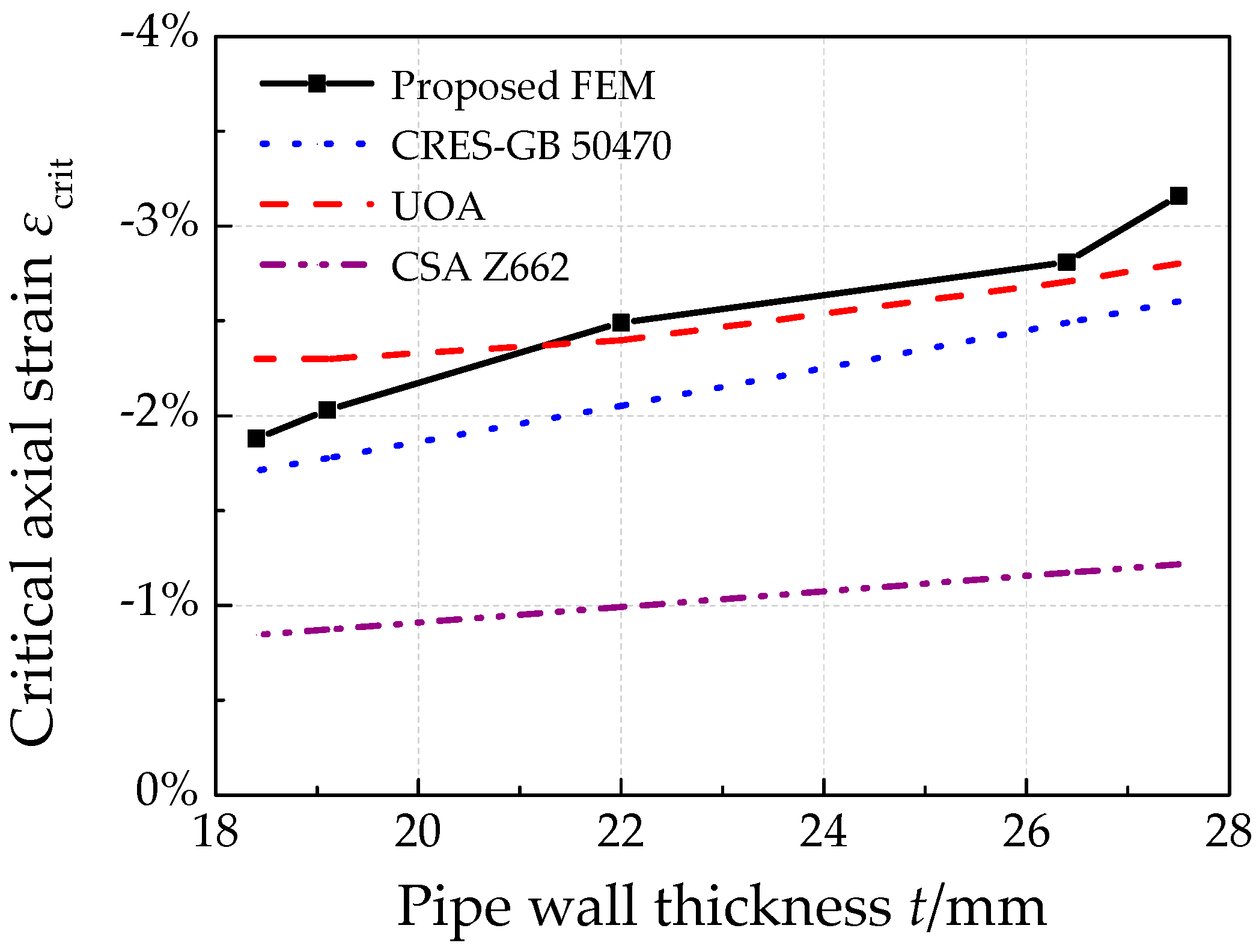
Results of the critical compressive strains of various pipe wall thicknesses derived by different methods are further compared in Figure 18. With increase of t, critical compressive strains increase monotonically. CSA Z662 model predicted results are also quite conservative. If t > 22 mm, the UOA model results has better agreement with the proposed numerical results. While if t ≤ 19.1 mm, the CRES-GB 50470 model has better agreement with the proposed numerical results. However, it should also be noted that, in generally, both the UOA model and the CRES-GB 50470 model have rather good prediction results for a large range of pipe wall thickness.
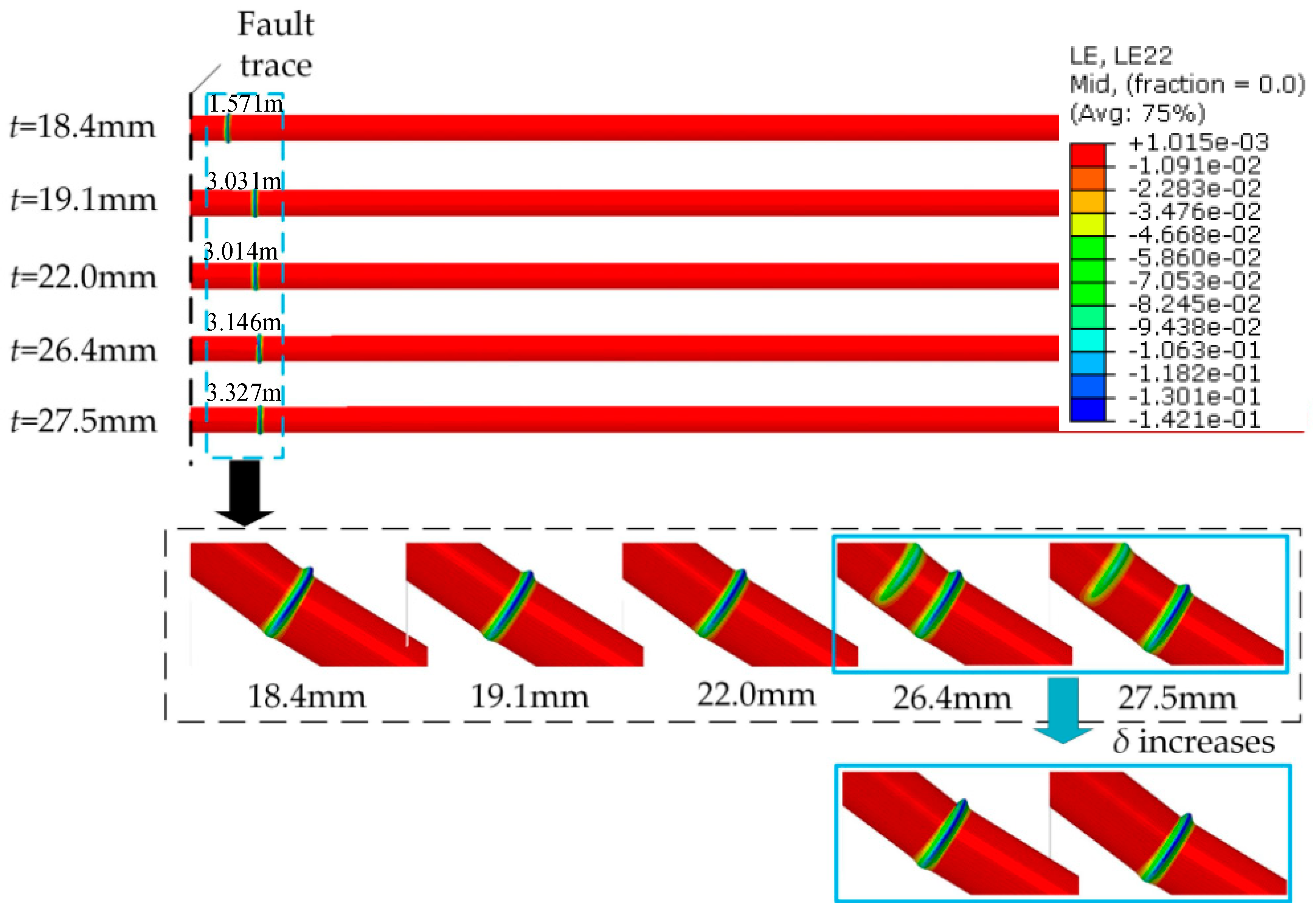
Figure 19 illustrates the post buckling results for pipes with different pipe wall thickness. For the pipes with t ≤ 22 mm, one wrinkle near the fault trace occurs after strain concentration induced by local buckling. For the pipe with t ≥ 26.4 mm, two wrinkles will first appear in the pipe after local buckling, and finally concentrate to the major wrinkle. The local failure position is located further away from the fault trace with the increase of pipe wall thickness.
4.5. Effects of Soil Parameters
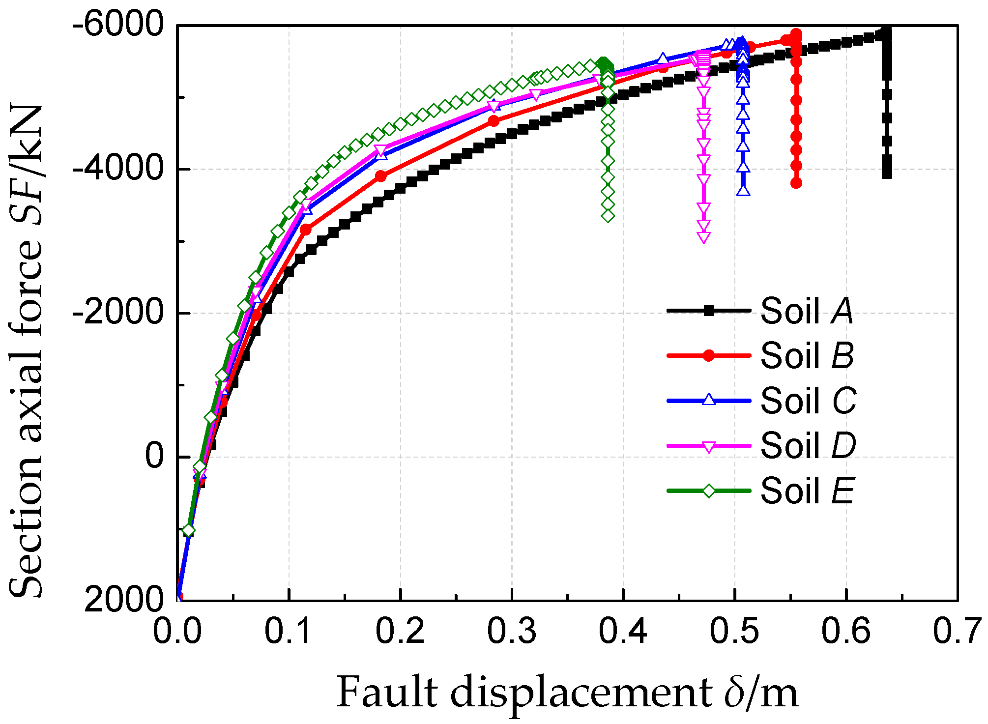
Buried pipelines are surrounded with soil. Constraints of soil on a pipe are directly related to the soil parameters as internal friction angle, cohesion, effective unit weight as well as the pipe soil friction coefficient according to ASCE-ALA Guideline [39]. In this section, five different kinds of clay with various parameters listed in Table 1 were considered to investigate the effects of soil constraints. The soil performed harder and has a larger resistance from Soil A to Soil E in sequence.
Figure 20 shows the trends of section axial force SF in the buckled area with fault displacement δ in various soil types. When δ < 0.05 m, the five curves are almost the same. After δ = 0.1 m, SF for pipe buried in Soil E is the largest one, and it first drops when δ reaches 0.39 m. The relationships of the critical fault displacements derived from Figure 20 with the soil type are further illustrated in Figure 21, which shows that a harder soil stiffness induces a relatively smaller critical fault displacement. Thus, pipes crossing active faults locating hard soil sites have higher failure risk of plastic local buckling.
The critical compressive strains derived by the presented model for different soil conditions are plotted in Figure 22, comparing with common failure criteria based on the case parameters. The results of the CSA Z662 model, UOA model and CRES-GB 50470 model are all constants, similar to Figure 10, because the presented critical compressive strain prediction models are all based on pipe’s pure bending test, which cannot consider the influences of external environment loads encountered by actual pipes in field. In addition, similar to the conclusions derived in the previous sections, the CSA model predicts rather conservative results. The UOA model and CRES-GB50470 model both have a good prediction, but the UOA model result is a little un-conservative. Furthermore, although εcrit derived by the numerical model is around 2%, it should be noted that with the increase of soil stiffness surrounding pipe, εcrit has a general decreasing tendency, which reflects that external load conditions should also affect some of pipe’s strain capacity.
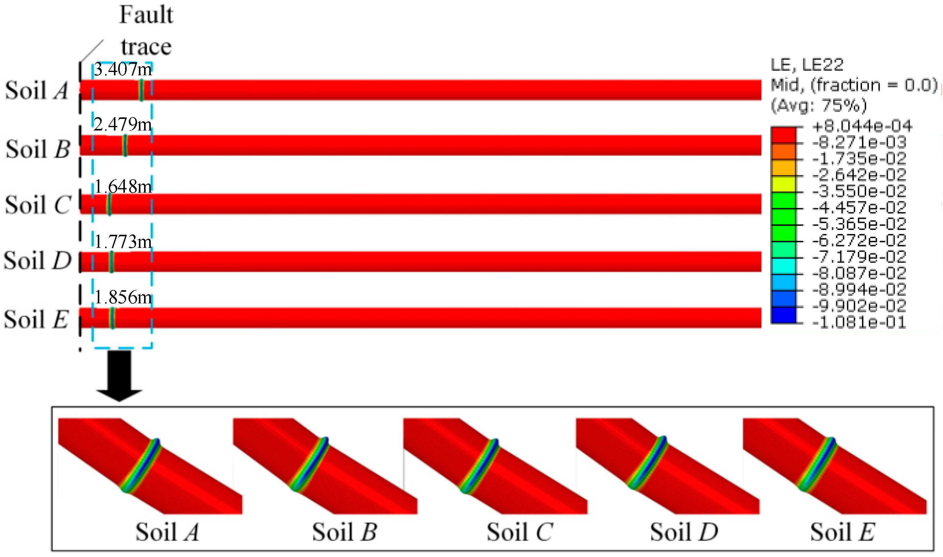
Post buckling axial strain contours of pipes buried in these five kinds of clay are compared in Figure 23. The pipes have almost same plastic section deformation with a bulge pattern induced by the operation pressure considered for all cases. However, variations exist between these five cases on the failure location. If the soil is relatively soft (i.e., Soil A–C), the local buckling failure position is located nearer the fault trace with a stiffer surrounding soil. However, if the soil is hard enough, harder than Soil C of the cases in this study, the local buckling failure position will have negligible variations for different soil types.
4.6. Effects of Pipe Buried Depth
Pipes are commonly buried in various depths according to the environment or pipe safety concern. In this section, five buried depth values, i.e., 0.5, 1.0, 1.5, 2.0, 3.0 m, possibly encountered in true engineering cases were adopted for parametric investigation. As illustrated in Figure 24, trends of SF with δ for pipes buried in different depth are the same, until the pipe buried in 3.0 m reaches its critical fault displacement (0.39 m), where its section axial force first drops. After that, pipe buckles in sequence from the deepest buried depth to shallowest buried depth. The quantitative relationship of the critical fault displacement δcrit with pipe buried depth H is displayed in Figure 25, which shows that δcrit decreases almost linearly with H, from 0.51 to 0.39 m, when H increases from 0.5 to 3 m. Thus, when subjected to fault displacement, a deeper buried depth of pipe enhances soil constraint on pipe leading to easier buckling failure in pipe.
Variations of the critical compressive strain in the pipe with buried depth are shown in Figure 26, which is quite similar with Figure 22. This is mainly because both increase of soil stiffness and increase of buried depth increase the soil resistance on pipe, which causes larger axial compression and lateral bending with the same fault displacement.
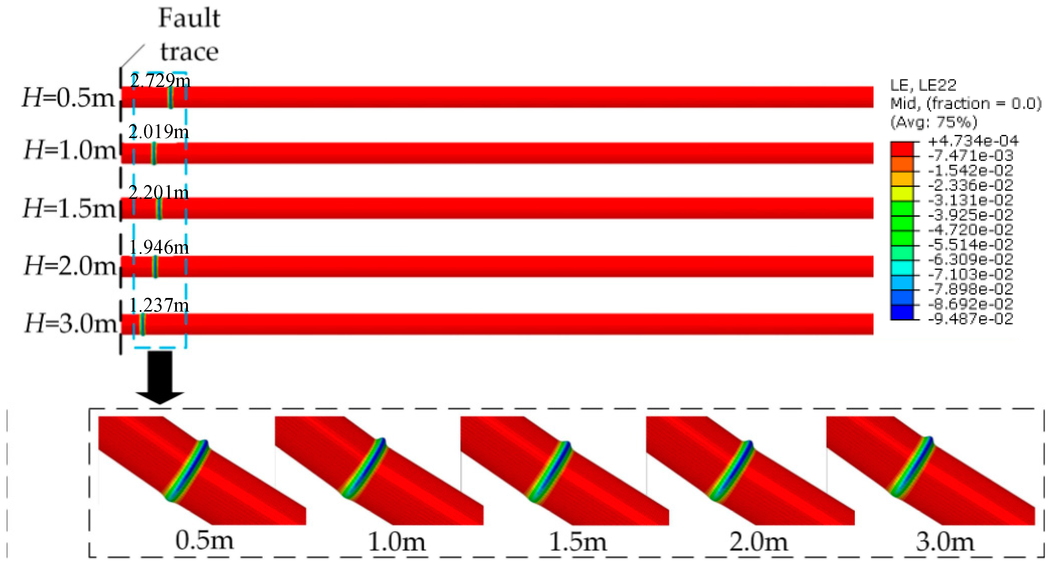
The plastic deformation of pipes in the post buckling stage with the considered five buried depths are plotted in Figure 27. The same elephant foot buckling phenomenon appears in all cases. In addition, with the increase of pipe buried depth, the local buckling failure position is located nearer the fault trace as the trends found in Figure 23 for relatively soft soil types.
5. Conclusions
Local buckling is a major failure type for buried steel pipelines subjected to active fault movements. Based on refined numerical model using finite element methods, it has been found that pipe subjected to strike-slip fault displacements incurs local buckling when it reaches the compressive limit state, which can be identified by the sudden drop of the section axial force in the buckled area. After buckling, wavy axial strain distribution appears initially and changes into strain concentration with wrinkling immediately. Effects of the pipe-fault intersection angle, pipe operation pressure, pipe wall thickness, soil parameters and pipe buried depth on the local buckling behavior of high-strength X80 pipes were further investigated through a parametric analysis. Some conclusions can be drawn:
- For compressive strike-slip fault, the critical fault displacement increases initially and decrease afterwards with pipe fault intersection angle. When pipe fault intersection angle equals 135°, the pipe is most likely to be buckled and fail. The failure section of pipe locates further with increase of pipe fault intersection angle.
- Pipe operation pressure decreases pipe’s anti-buckling capacity generally, although a positive correlation between the critical compressive strain and pipe operation pressure was also found. In addition, operation pressure affects pipe’s plastic deformation shape in post buckling stage. For the pipe investigated, when P is larger than 4 MPa, the pipe performs an elephant’s foot buckling, and when P is 0 MPa, the pipe exhibits diamond buckling.
- Pipe wall thickness has a positive relationship with both the critical fault displacement and critical axial strain for pipe. The failure pipe section of thicker pipes locates further away from fault trace.
- Both increasing soil stiffness and pipe buried depth increase soil constraints on pipe, which will lead to a smaller critical fault displacement. In addition, pipe failure locations are nearer to fault trace with stronger constraints by surrounding soil.
- For pure pipes without considering the geometry imperfections, the CSA Z662 model predicts too conservative results for compressive strain capacity. Generally, both the CRES-GB 50470 model and the UOA model have rather good critical compressive strain results compared with the numerical derived results for various conditions. Among them, the CRES-GB 50470 model is recommended for pipe failure assessment, because it is relatively conservative.
- Numerical results show that not only the pipe parameters (i.e., geometrical parameters and internal pressure) but also external loads (pipe fault intersection angle, soil constraints on pipe) also have some minor effects on pipe’s critical compressive strain, which is not considered by the commonly available buckling failure criteria.
Acknowledgments
This research has been co-financed by China National Key Research and Development Project under (Grant No. 2016YFC0802105), National Natural Science Foundation of China (Grant No. 51309236).
Author Contributions
Hong Zhang conceived and designed the physical model. Xiaoben Liu established the numerical model and wrote the paper. Baodong Wang, Kai Wu and Qian Zheng performed the numerical analysis. Mengying Xia and Yinshan Han analyzed the data.
Conflicts of Interest
The authors declare no conflict of interest.
Nomenclature
| D | the pipe diameter (m) |
| t | the pipe wall thickness (m) |
| P | the pipe operation pressure (MPa) |
| the compressive strain capacity of steel pipes | |
| σy | the yield strength of pipe steel (MPa) |
| E | the initial elastic modulus (MPa) |
| hg | the height of the geometry imperfection (mm) |
| σu | the tensile strength of pipe material (MPa) |
| σa | the applied net-section stress in the longitudinal direction of pipe (MPa) |
| Tu | the axial peak resistant force per unit length of soil springs (kN/m) |
| Pu | the lateral peak resistant force per unit length of soil springs (kN/m) |
| Qu | the vertical uplift peak resistant force per unit length of soil springs (kN/m) |
| Qd | the vertical bearing peak resistant force per unit length of soil springs (kN/m) |
| Δt | the yield displacement in the axial direction (m) |
| Δp | the yield displacement in the lateral direction (m) |
| Δqu | the yield displacement in the vertical uplift direction (m) |
| Δqd | the yield displacement in the vertical bearing direction (m) |
| σtrue | the true stress (MPa) |
| εtrue | the true strain |
| r | the strain hardening exponent |
| α | the yield offset parameter |
| A | the pipe cross section area (m2) |
| ΔL | the pipe extension at Point B (m) |
| δ | the fault displacement (m) |
| ΔX | the fault displacement in the pipe axial direction (m) |
| ΔY | the fault displacement in the pipe perpendicular direction (m) |
| β | the pipe fault intersection angle (°) |
| εcrit | the critical compressive strain |
| SF | the section axial force in buckled area (kN) |
| SFcrit | the critical section axial force in buckled area (kN) |
| K | the coefficient of theory critical axial force |
| εaxial | the axial compressive strain |
| δcrit | the critical fault displacements (m) |
| the internal friction angle of the soil (°) | |
| c | the soil cohesion representative (kPa) |
| γ | the effective unit weight of soil (kN/m3) |
| f | the pipe–soil friction coefficient |
| H | the pipe buried depth (m) |
References
- Lower, M.D. Strain-Based Design Methodology of Large Diameter Grade X80 Linepipe. Ph.D. Thesis, University of Tennessee, Knoxville, TN, USA, 2014. [Google Scholar]
- Liu, X.B.; Zhang, H.; Wu, K.; Xia, M.Y.; Chen, Y.F.; Li, M. Buckling failure mode analysis of buried X80 steel gas pipeline under reverse fault displacement. Eng. Fail. Anal. 2017, 77, 50–64. [Google Scholar] [CrossRef]
- Newmark, N.M.; Hall, W.J. Pipeline design to resist large fault displacement. In Proceedings of the U.S. National Conference on Earthquake Engineering, Ann Arbor, MI, USA, 18–20 June 1975; pp. 416–425. [Google Scholar]
- Kennedy, R.P.; Chow, A.W.; Williamson, R.A. Fault movement effects on buried oil pipeline. Transp. Eng. J. 1977, 103, 617–633. [Google Scholar]
- Wang, R.L.; Yeh, Y.H. A refined seismic analysis and design of buried pipeline for fault movement. Earthq. Eng. Struct. Dyn. 1985, 13, 75–96. [Google Scholar] [CrossRef]
- Karamitros, D.K.; Bouckovalas, G.D.; Kouretzis, G.P. Stress analysis of buried steel pipelines at strike-slip fault crossings. Soil Dyn. Earthq. Eng. 2007, 27, 200–211. [Google Scholar] [CrossRef]
- Trifonov, O.V.; Cherniy, V.P. A semi-analytical approach to a nonlinear stress-strain analysis of buried steel pipelines crossing active faults. Soil Dyn. Earthq. Eng. 2010, 30, 1298–1308. [Google Scholar] [CrossRef]
- Zhang, L.; Zhao, X.; Yan, X.; Yang, X. Elastoplastic analysis of mechanical response of buried pipelines under strike-slip faults. Int. J. Geomech. 2016, 17. [Google Scholar] [CrossRef]
- Ha, D.; Abdoun, T.H.; O’Rourke, M.J.; Symans, M.D.; O’Rourke, T.D.; Palmer, M.C.; Steward, H.E. Buried high-density polyethylene pipelines subjected to normal and strike-slip faulting-a centrifuge investigation. Can. Geotech. J. 2008, 45, 1733–1742. [Google Scholar] [CrossRef]
- Ha, D.; Abdoun, T.H.; O’Rourke, M.J.; Symans, M.D. Centrifuge modeling of earthquake effects on buried high-density polyethylene (HDPE) pipelines crossing fault zones. J. Geotech. Geoenviron. Eng. 2008, 134, 1501–1515. [Google Scholar] [CrossRef]
- O’Rourke, T.D.; Jung, J.K.; Argyrou, C. Underground pipeline response to earthquake-induced ground deformation. Soil Dyn. Earthq. Eng. 2016, 91, 272–283. [Google Scholar] [CrossRef]
- Jung, J.K.; O’Rourke, T.D.; Argyrou, C. Multi-directional force–displacement response of underground pipe in sand. Can. Geotech. J. 2016, 53, 1763–1781. [Google Scholar] [CrossRef]
- Jalali, H.H.; Rofooei, F.R.; Attari, N.K.A. Performance of Buried Gas Distribution Pipelines Subjected to Reverse Fault Movement. J. Earthq. Eng. 2017, 10, 1–24. [Google Scholar] [CrossRef]
- Jalali, H.H.; Rofooei, F.R.; Attari, N.K.A.; Samadian, M. Experimental and finite element study of the reverse faulting effects on buried continuous steel gas pipelines. Soil Dyn. Earthq. Eng. 2016, 86, 1–14. [Google Scholar] [CrossRef]
- Rofooei, F.R.; Jalali, H.H.; Attari, N.K.A.; Kenarangi, H.; Samadian, M. Parametric study of buried steel and high density polyethylene gas pipelines due to oblique-reverse faulting. Can. J. Civ. Eng. 2015, 42, 178–189. [Google Scholar] [CrossRef]
- Trifonov, O.V. Numerical stress-strain analysis of buried steel pipelines crossing active strike-slip faults with an emphasis on fault modeling aspects. J. Pipeline Syst. Eng. Pract. 2015, 6. [Google Scholar] [CrossRef]
- Xie, X.J.; Symans, M.D.; O’Rourke, M.J.; Abdoun, T.H.; O’Rourke, T.D.; Palmer, M.C.; Stewart, H.E. Numerical modeling of buried HDPE pipelines subjected to normal faulting: A case study. Earthq. Spectra 2013, 29, 609–632. [Google Scholar] [CrossRef]
- Xie, X.J.; Symans, M.D.; O’Rourke, M.J.; Abdoun, T.H.; O’Rourke, T.D.; Palmer, M.C.; Stewart, H.E. Numerical modeling of buried HDPE pipelines subjected to strike-slip faulting. J. Earthq. Eng. 2011, 15, 1273–1296. [Google Scholar] [CrossRef]
- Joshi, S.; Prashant, A.; Deb, A.; Jain, S.K. Analysis of buried pipelines subjected to reverse fault motion. Soil Dyn. Earthq. Eng. 2011, 31, 930–940. [Google Scholar] [CrossRef]
- Uckan, E.; Akbas, B.; Shen, J.; Rou, W.; Paolacci, W.; O’Rourke, M. A simplified analysis model for determining the seismic response of buried steel pipes at strike-slip fault crossings. Soil Dyn. Earthq. Eng. 2015, 75, 55–65. [Google Scholar] [CrossRef]
- Liu, X.B.; Zhang, H.; Han, Y.S.; Xia, M.Y.; Zheng, W. A semi-empirical model for peak strain prediction of buried X80 steel pipelines under compression and bending at strike-slip fault crossings. J. Nat. Gas Sci. Eng. 2016, 32, 465–475. [Google Scholar] [CrossRef]
- Melissianos, V.E.; Vamvatsikos, D.; Gantes, C.J. Performance assessment of buried pipelines at fault crossings. Earthq. Spectra 2017, 33, 201–218. [Google Scholar] [CrossRef]
- Melissianos, V.E.; Vamvatsikos, D.; Gantes, C.J. Performance-based assessment of protection measures for buried pipes at strike-slip fault crossings. Soil Dyn. Earthq. Eng. 2017, 101, 1–11. [Google Scholar] [CrossRef]
- Liu, X.B.; Zhang, H.; Gu, X.T.; Chen, Y.F.; Xia, M.Y.; Wu, K. Strain demand prediction method for buried X80 steel pipelines crossing oblique-reverse faults. Earthq. Struct. 2017, 12, 321–332. [Google Scholar] [CrossRef]
- Xu, L.; Lin, M. Analysis of buried pipelines subjected to reverse fault motion using the vector form intrinsic finite element method. Soil Dyn. Earthq. Eng. 2017, 93, 61–83. [Google Scholar] [CrossRef]
- Kaya, E.S.; Uckan, E.; O’Rourke, M.J.; Karamanos, S.A.; Akbas, B.; Cakir, F.; Cheng, Y. Failure analysis of a welded steel pipe at Kullar fault crossing. Eng. Fail. Anal. 2016, 71, 43–62. [Google Scholar] [CrossRef]
- Zhang, J.; Liang, Z.; Han, C.J. Buckling behavior analysis of buried gas pipeline under strike-slip fault displacement. J. Nat. Gas Sci. Eng. 2014, 21, 921–928. [Google Scholar] [CrossRef]
- Zhang, J.; Liang, Z.; Han, C.J.; Zhang, H. Numerical simulation of buckling behavior of the buried steel pipeline under reverse fault displacement. Mech. Sci. 2015, 6, 203–210. [Google Scholar] [CrossRef]
- Vazouras, P.; Karamanos, S.A.; Dakoulas, P. Finite element analysis of buried steel pipelines under strike-slip fault displacements. Soil Dyn. Earthq. Eng. 2010, 30, 1361–1376. [Google Scholar] [CrossRef]
- Vazouras, P.; Karamanos, S.A.; Dakoulas, P. Mechanical behavior of buried steel pipes crossing active strike-slip faults. Soil Dyn. Earthq. Eng. 2012, 41, 164–180. [Google Scholar] [CrossRef]
- Vazouras, P.; Dakoulas, P.; Karamanos, S.A. Pipe-soil interaction and pipeline performance under strike-slip fault movements. Soil Dyn. Earthq. Eng. 2015, 72, 48–65. [Google Scholar] [CrossRef]
- Vazouras, P.; Karamanos, S.A. Structural behavior of buried pipe bends and their effect on pipeline response in fault crossing areas. Bull. Earthq. Eng. 2017, 4, 1–26. [Google Scholar] [CrossRef]
- Liu, X.B.; Zhang, H.; Li, M.; Xia, M.Y.; Zheng, W.; Wu, K.; Han, Y.S. Effects of steel properties on the local buckling response of high strength pipelines subjected to reverse faulting. J. Nat. Gas Sci. Eng. 2016, 33, 378–387. [Google Scholar] [CrossRef]
- Kainat, M.; Lin, M.; Cheng, J.R.; Martens, M.; Adeeb, S. Effects of the initial geometric imperfections on the buckling behavior of high-strength UOE manufactured steel pipes. J. Press. Vessel Technol. 2016, 138. [Google Scholar] [CrossRef]
- Neupane, S.; Adeeb, S.; Cheng, R.; Ferguson, J.; Martens, M. Modeling the deformation response of high strength steel pipelines—Part I: Material characterization to model the plastic anisotropy. J. Appl. Mech. 2012, 136, 272–275. [Google Scholar] [CrossRef]
- Neupane, S.; Adeeb, S.; Cheng, R.; Ferguson, J.; Martens, M. Modeling the deformation response of high strength steel pipelines—Part II: Effects of material characterization on the deformation response of pipes. J. Appl. Mech. 2012, 79, 051003. [Google Scholar] [CrossRef]
- Canadian Standard Association (CSA). Oil and Gas Pipeline Systems; CSA Standard; CSA Z662-11; Canadian Standard Association: Mississauga, ON, Canada, 2015. [Google Scholar]
- Gresnigt, A.M. Plastic Design of Buried Steel Pipelines in Settlement Areas; STEVIN-laboratory of the Department of Civil Engineering, Delft University of Technology: Delft, The Netherlands, 1987. [Google Scholar]
- American Lifelines Alliance. American Society of Civil Engineers, Guidelines for the Design of Buried Steel Pipe (with Addenda through February 2005); American Lifelines Alliance: Reston, VA, USA, 2005. [Google Scholar]
- Indian Institute of Technology Kanpur. IITK-GSDMA Guidelines for Seismic Design of Buried Pipelines, Gandhinagar: Gujarat State Disaster Management Authority; Indian Institute of Technology Kanpur: Kalyanpur, India, 2007. [Google Scholar]
- Dorey, A.B.; Murray, D.W.; Cheng, J.J.R. Critical buckling strain equations for energy pipelines—A parametric study. J. Offshore Mech. Arct. Eng. 2006, 128, 248–255. [Google Scholar] [CrossRef]
- Liu, M.; Wang, Y.Y.; Zhang, F.; Kotian, K. Realistic Strain Capacity Models for Pipeline Construction and Maintenance; US DOT PHMSA Other Transaction Agreement #DTPH56-10-T-000016, Draft Final Report; Center For Reliable Energy Systems: Dublin, OH, USA, 2013. [Google Scholar]
- Codeofchina Inc. GB 50470-2008 Seismic Technical Code for Oil and Gas Transmission Pipeline Engineering; Codeofchina Inc.: Beijing, China, 2017. [Google Scholar]
- American Petroleum Institute (API). Design, Construction, Operation, and Maintenance of Offshore Hydrocarbon Pipelines (Limit State Design); API Recommended Practice, API RP 1111; American Petroleum Institute: Washington, DC, USA, 1991. [Google Scholar]
- Det Norske Veritas (DNV). Submarine Pipeline Systems; DNV Offshore Standard, DNV-OS-F101; Det Norske Veritas: Oslo, Norway, 2010. [Google Scholar]
- Committee on Gas and Liquid Fuel Lifelines of the American Society of Civil Engineers Technical Council on Lifeline Earthquake Engineering. Guidelines for the Seismic Design of Oil and Gas Pipeline Systems; ASCE: Reston, VA, USA, 1984; pp. 10–12. [Google Scholar]
- Hibbitt, D.; Karlsson, B.; Sorensen, P. ABAQUS Standard User’s and Reference Manuals; Version 6.14; Hibbitt, Karlsson & Sorensen, Inc.: Johnston, RI, USA, 2007. [Google Scholar]
- Ramberg, W.; Osgood, W.R. Description of Stress-Strain Curves by Three Parameters; NACA Technical Note; No. 902; National Advisory Committee for Aeronautics (NACA): Washington, DC, USA, 1943.
- Liu, X.B.; Zhang, H.; Xia, M.Y. Buckling behavior of buried steel pipeline under compression strike-slip fault. In Proceedings of the 2017 ASME Pressure Vessels & Piping Conference, Waikoloa, HI, USA, 16–20 July 2017. [Google Scholar]
- Martini, A.; Troncossi, M.; Rivola, A. Leak Detection in Water-Filled Small-Diameter Polyethylene Pipes by Means of Acoustic Emission Measurements. Appl. Sci. 2017, 7, 2. [Google Scholar] [CrossRef]
- Juliano, T.M.; Meegoda, J.N.; Watts, D.J. Acoustic Emission Leak Detection on a Metal Pipeline Buried in Sandy Soil. J. Pipeline Syst. Eng. Pract. 2013, 4, 149–155. [Google Scholar] [CrossRef]
- Martini, A.; Troncossi, M.; Rivola, A. Vibroacoustic Measurements for Detecting Water Leaks in Buried Small-Diameter Plastic Pipes. J. Pipeline Syst. Eng. Pract. 2017, 8, 1–10. [Google Scholar] [CrossRef]
- Yazdekhasti, S.; Piratla, K.R.; Atamturktur, S.; Khan, A. Experimental evaluation of a vibration-based leak detection technique for water pipelines. Struct. Infrastruct. Eng. 2017, 14, 46–55. [Google Scholar] [CrossRef]
- Liu, A.; Hu, Y.; Zhao, F.; Li, X.; Takada, S.; Zhao, L. An equivalent-boundary method for the shell analysis of buried pipelines under fault movement. Acta Seismol. Sin. 2004, 17, 150–156. [Google Scholar] [CrossRef]
- American Society of Mechanical Engineers. Pipeline Transportation Systems for Liquid Hydro Carbons and Other Liquids; ANSI/ASME2016, B31:4; American Society of Mechanical Engineers: New York, NY, USA, 2016. [Google Scholar]
- American Society of Mechanical Engineers. Gas Transmission and Distribution Piping Systems; ANSI/ASME2016, B31:8; American Society of Mechanical Engineers: New York, NY, USA; 2016. [Google Scholar]
Figure 1.
Schematic diagram of nonlinear soil springs on pipe, T for axial springs, P for lateral springs, and Q for vertical springs [39].
Figure 1.
Schematic diagram of nonlinear soil springs on pipe, T for axial springs, P for lateral springs, and Q for vertical springs [39].
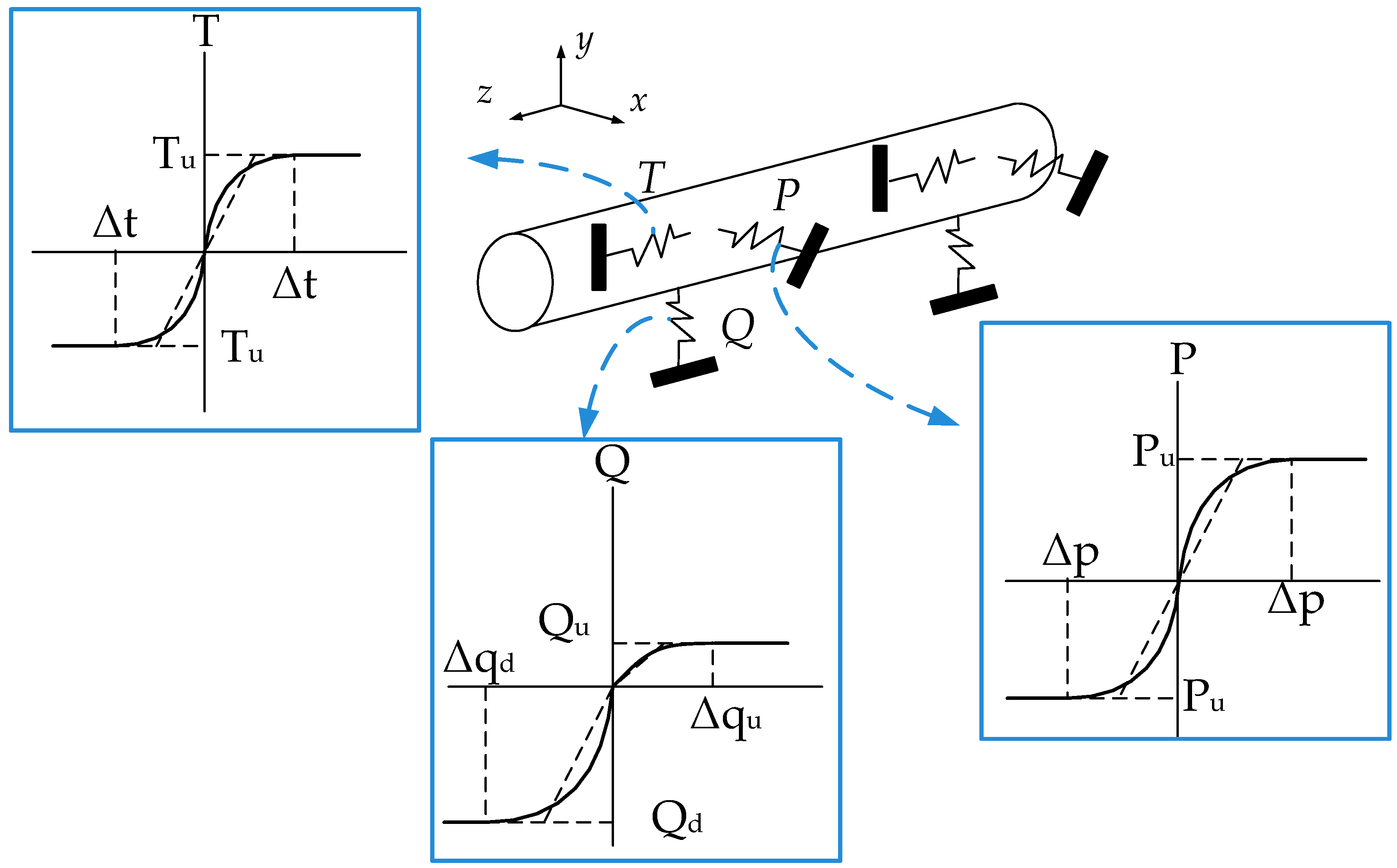
Figure 2.
Established finite element model for pipeline crossing strike slip faults.

Figure 3.
True stress strain curve of X80 line pipe steel.

Figure 4.
Constitutive model for the equivalent boundary spring.

Figure 5.
Comparison of strain distributions at cross-section where buckling occurs when δ = 0.61 m. (a) Longitudinal strain distribution; (b) Circumferential strain distribution.
Figure 5.
Comparison of strain distributions at cross-section where buckling occurs when δ = 0.61 m. (a) Longitudinal strain distribution; (b) Circumferential strain distribution.

Figure 6.
Trends of section axial force and axial strain in buckled area with fault displacement.
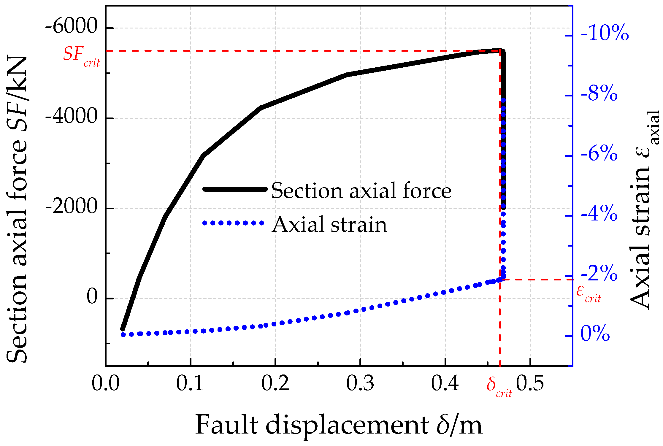
Figure 7.
Section axial force and axial strain distribution in pipe at various fault displacements.
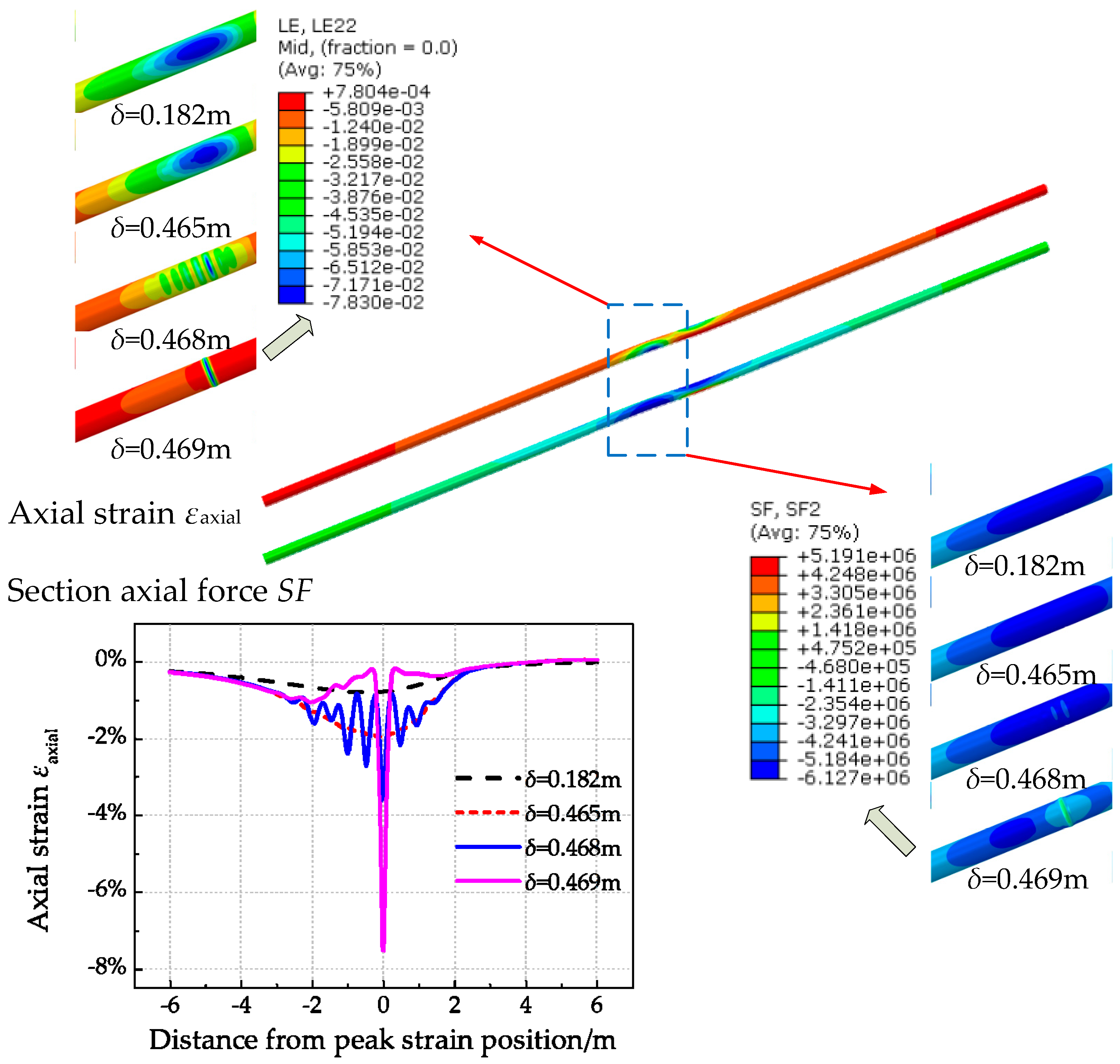
Figure 8.
Relationship between section axial force and fault displacement at different intersection angles.
Figure 8.
Relationship between section axial force and fault displacement at different intersection angles.
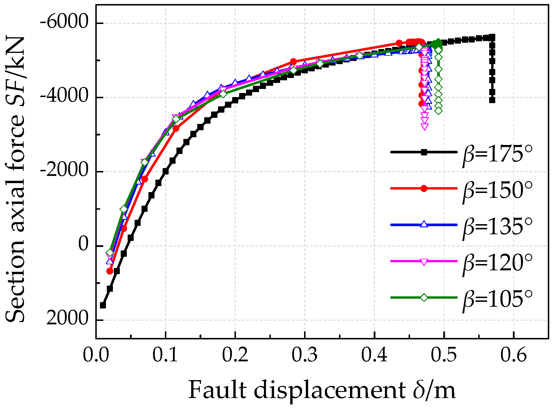
Figure 9.
Relationships of the critical fault displacement and the intersection angle.
Figure 10.
Relationships of the critical compressive strain and the intersection angles.
Figure 11.
Post buckling behavior (axial strain contour) of pipeline at various intersection angles.
Figure 11.
Post buckling behavior (axial strain contour) of pipeline at various intersection angles.
Figure 12.
Relationship between section axial force and fault displacement with different operation pressure.
Figure 12.
Relationship between section axial force and fault displacement with different operation pressure.
Figure 13.
Relationships of the critical fault displacements with the operation pressure.
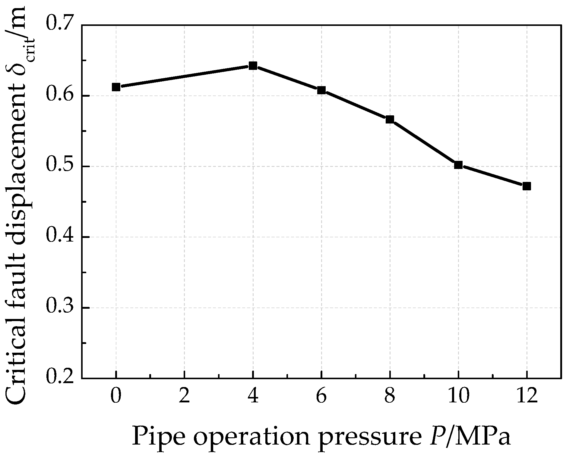
Figure 14.
Relationships of the critical compressive strains with the operation pressure.
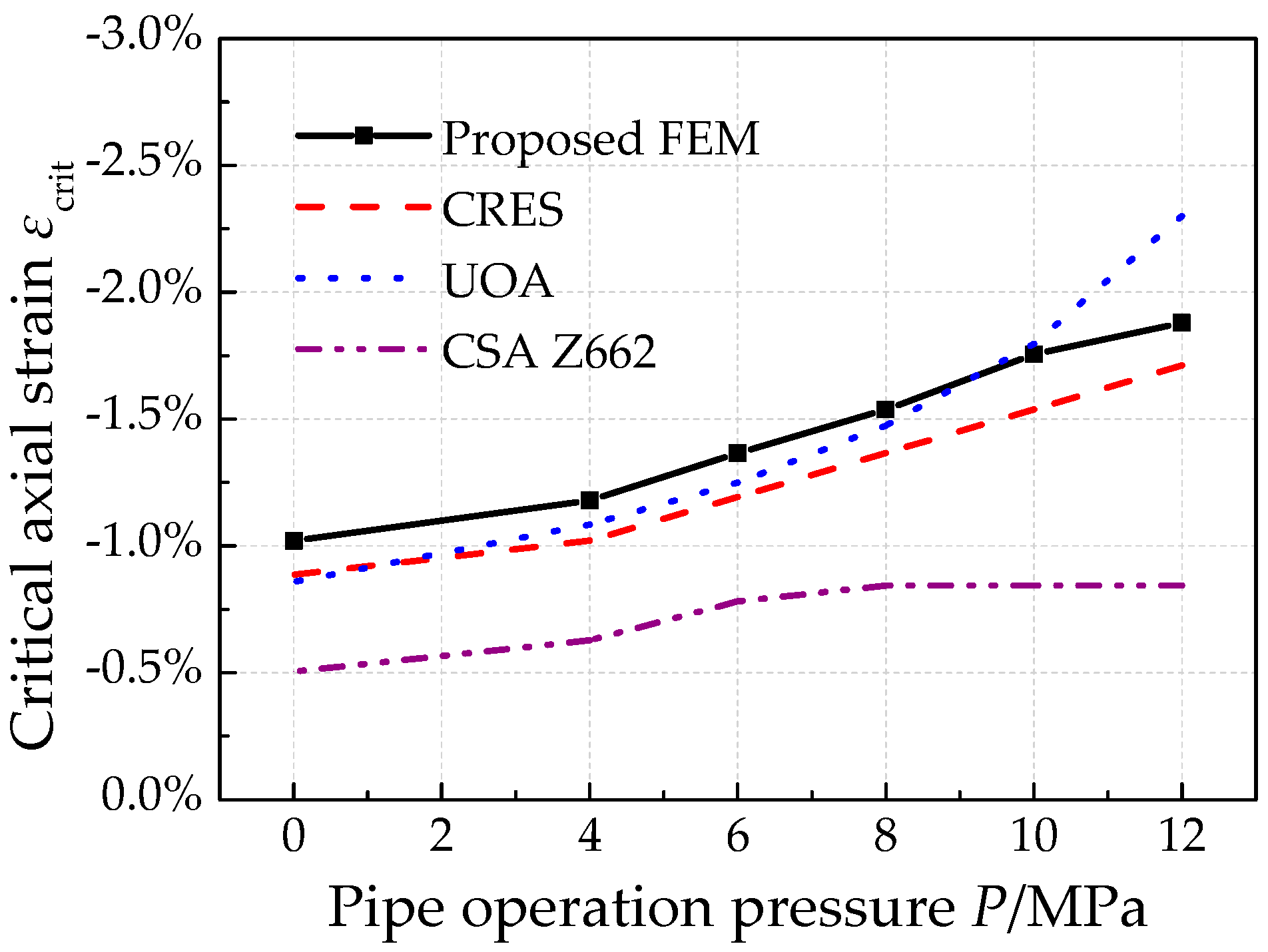
Figure 15.
Post buckling behavior (axial strain contour) of pipeline with different operation pressure.
Figure 15.
Post buckling behavior (axial strain contour) of pipeline with different operation pressure.
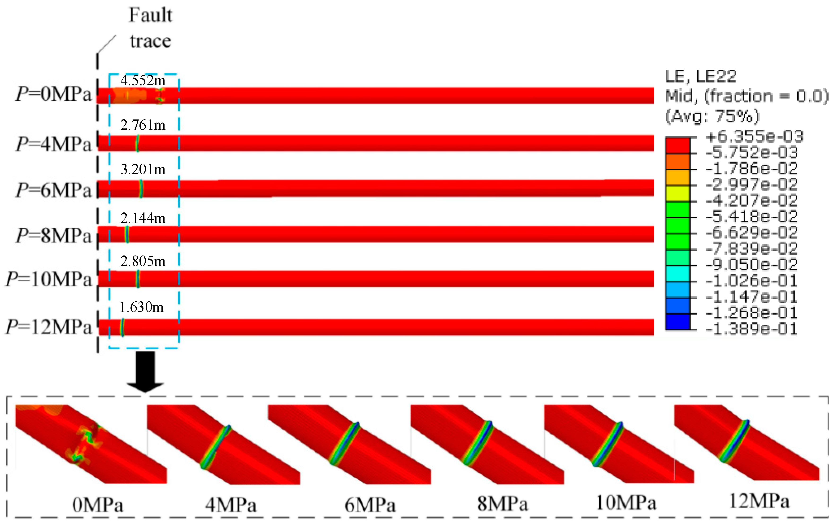
Figure 16.
Relationship between section axial force and fault displacement with different pipe wall thickness.
Figure 16.
Relationship between section axial force and fault displacement with different pipe wall thickness.
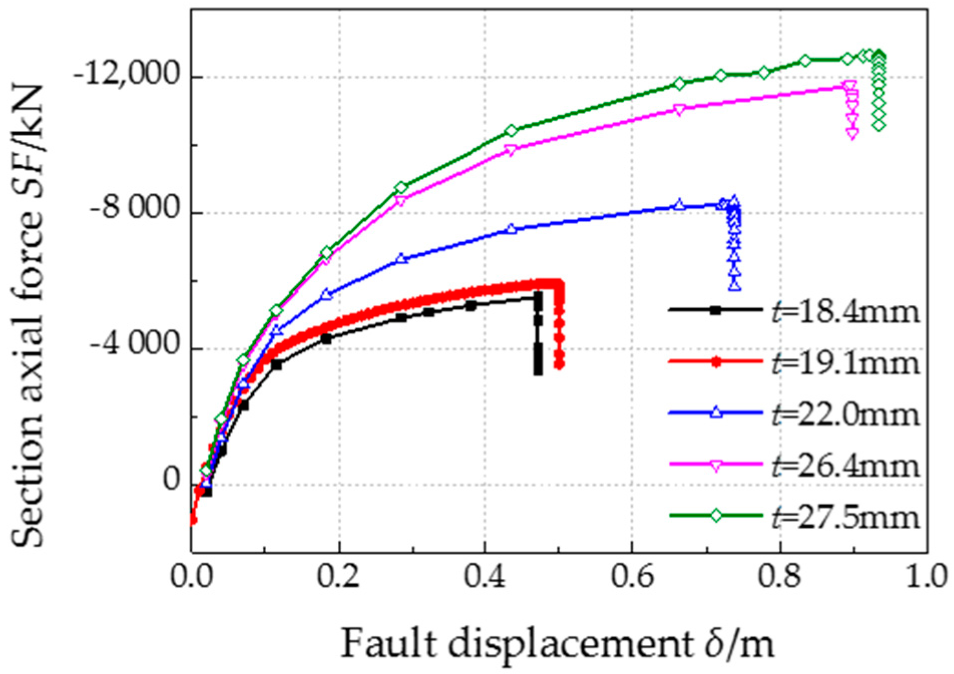
Figure 17.
Relationships of the critical fault displacements with the pipe wall thickness.
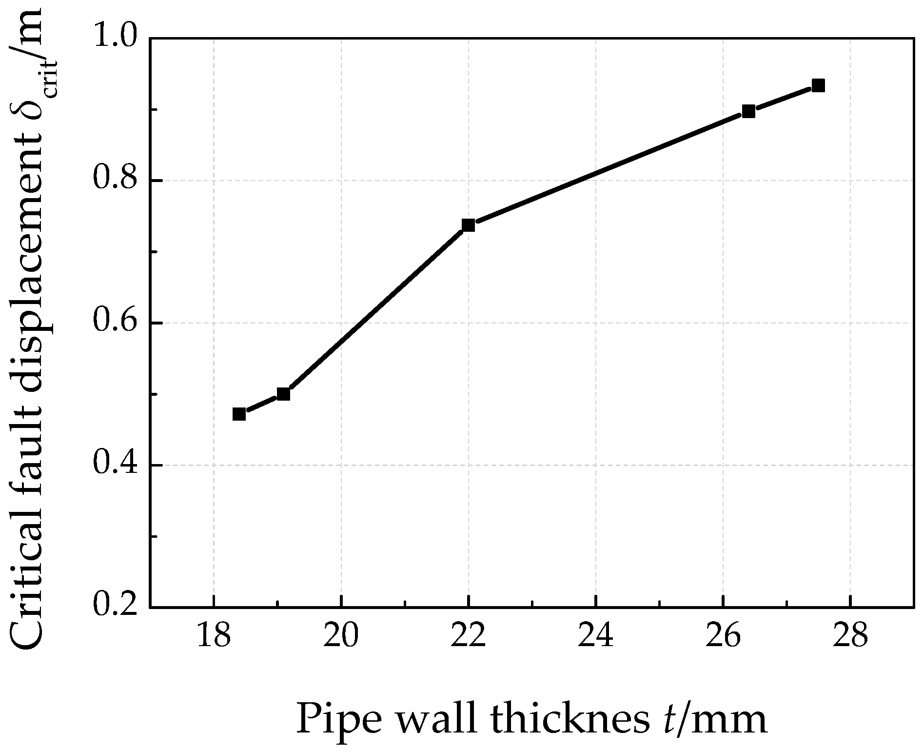
Figure 18.
Relationships of the critical compressive strains with the pipe wall thickness.

Figure 19.
Post buckling behavior (axial strain contour) of pipeline with different wall thickness.

Figure 20.
Relationship between section axial force and fault displacement with different soil parameters.
Figure 20.
Relationship between section axial force and fault displacement with different soil parameters.

Figure 21.
Relationships of the critical fault displacements with different soil parameters.
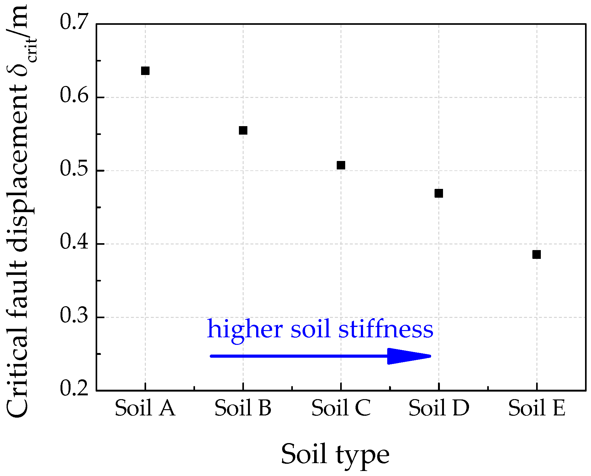
Figure 22.
Relationships of the critical compressive strains for different soil parameters.
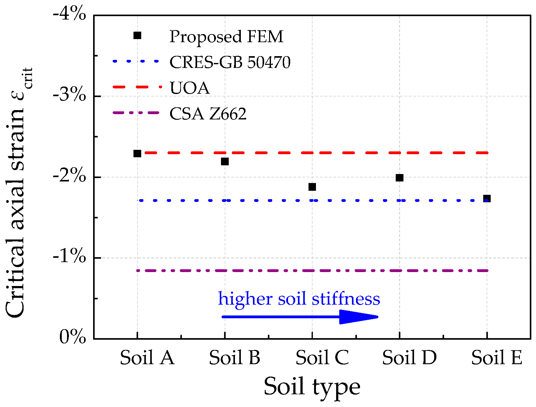
Figure 23.
Post buckling behavior (axial strain contour) of pipeline with different soil parameters.
Figure 23.
Post buckling behavior (axial strain contour) of pipeline with different soil parameters.

Figure 24.
Relationship between section axial force and fault displacement with different buried depths.
Figure 24.
Relationship between section axial force and fault displacement with different buried depths.
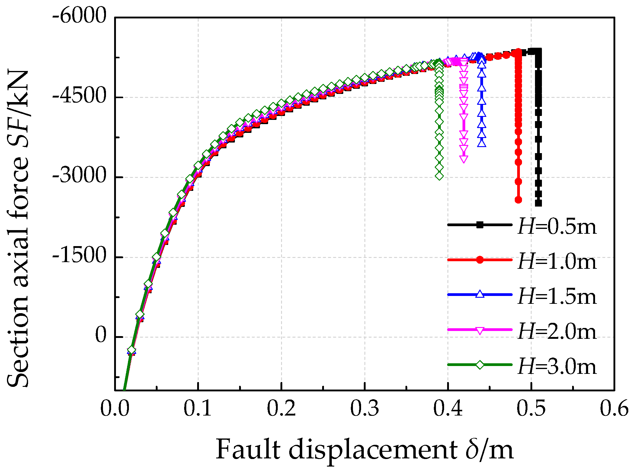
Figure 25.
Relationship of critical fault displacements with buried depth.
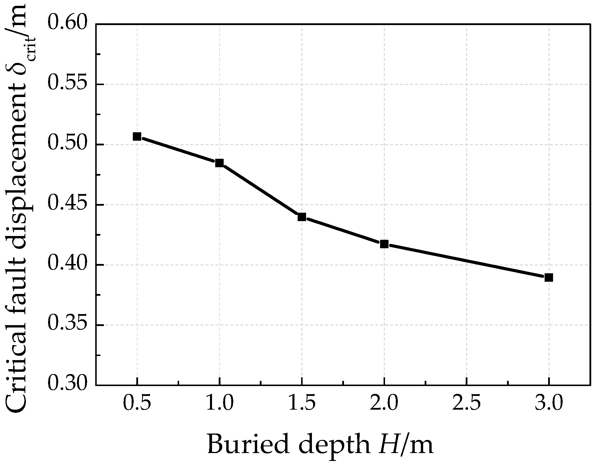
Figure 26.
Relationships of critical compressive strains with buried depth.
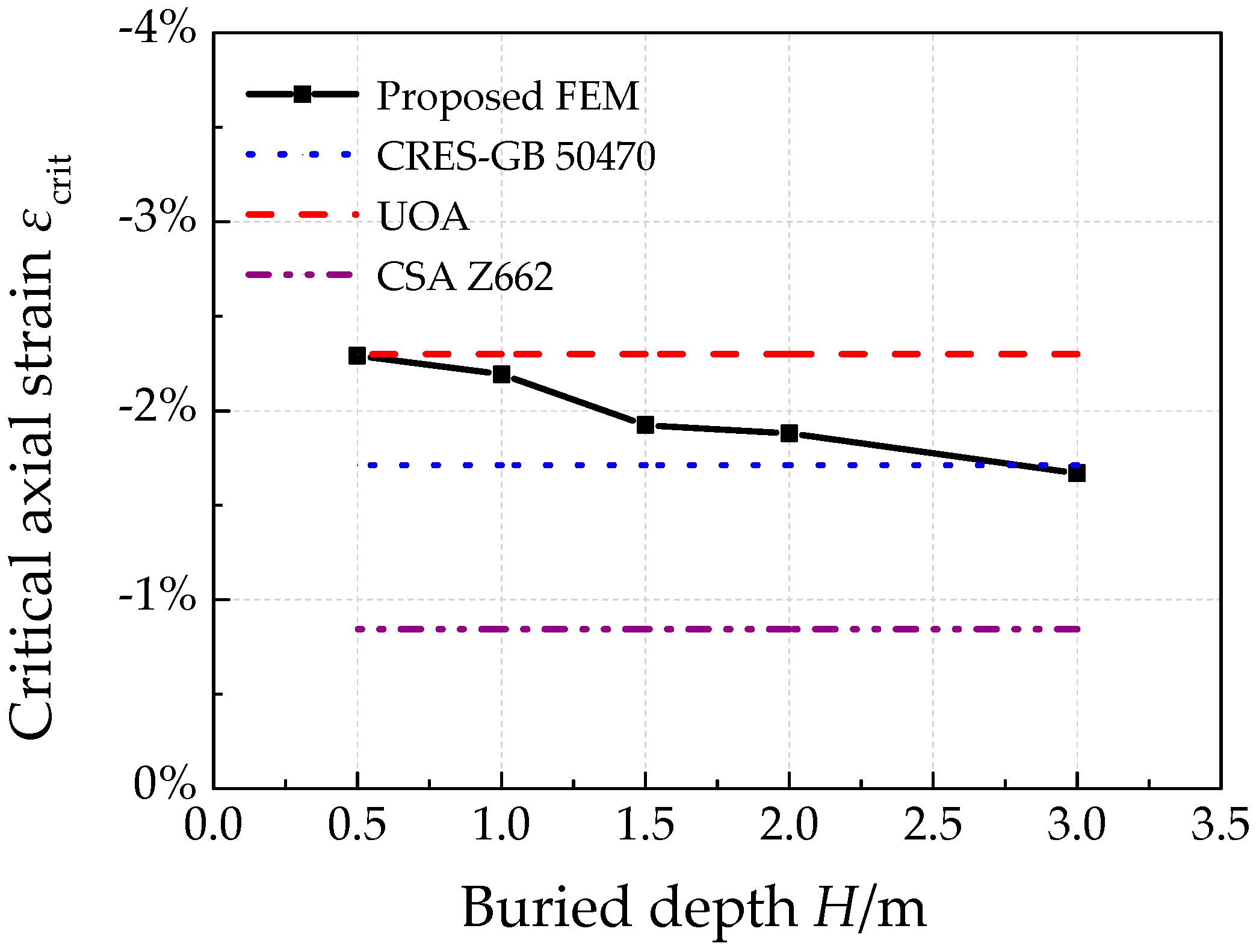
Figure 27.
Post buckling behavior (axial strain contour) of pipeline with different buried depth.


Table 1.
Soil parameters of different types of soil sites in numerical investigation used for pipe soil interaction.
Table 1.
Soil parameters of different types of soil sites in numerical investigation used for pipe soil interaction.
| Soil Sites Type | Internal Friction Angle ψ (°) | Cohesion c (kPa) | Effective Unit Weight of Soil γ (kN/m3) | Pipe-Soil Friction Coefficient f |
|---|---|---|---|---|
| Soil A | 30 | 30 | 22 | 0.6 |
| Soil B | 30 | 40 | 22 | 0.6 |
| Soil C | 33 | 50 | 22 | 0.6 |
| Soil D | 33 | 60 | 22 | 0.6 |
| Soil E | 33 | 70 | 22 | 0.6 |
© 2017 by the authors. Licensee MDPI, Basel, Switzerland. This article is an open access article distributed under the terms and conditions of the Creative Commons Attribution (CC BY) license (http://creativecommons.org/licenses/by/4.0/).
Share and Cite
MDPI and ACS Style
Liu, X.; Zhang, H.; Wang, B.; Xia, M.; Wu, K.; Zheng, Q.; Han, Y. Local Buckling Behavior and Plastic Deformation Capacity of High-Strength Pipe at Strike-Slip Fault Crossing. Metals 2018, 8, 22. https://doi.org/10.3390/met8010022
AMA Style
Liu X, Zhang H, Wang B, Xia M, Wu K, Zheng Q, Han Y. Local Buckling Behavior and Plastic Deformation Capacity of High-Strength Pipe at Strike-Slip Fault Crossing. Metals. 2018; 8(1):22. https://doi.org/10.3390/met8010022
Chicago/Turabian StyleLiu, Xiaoben, Hong Zhang, Baodong Wang, Mengying Xia, Kai Wu, Qian Zheng, and Yinshan Han. 2018. "Local Buckling Behavior and Plastic Deformation Capacity of High-Strength Pipe at Strike-Slip Fault Crossing" Metals 8, no. 1: 22. https://doi.org/10.3390/met8010022
Note that from the first issue of 2016, this journal uses article numbers instead of page numbers. See further details here.