Quadratic Midpoint Integration Method for J2 Metal Plasticity

Department of Civil Engineering, Chonnam National University, 77 Yongbong-Ro, Gwangju 61186, Korea
*
Author to whom correspondence should be addressed.
Metals 2018, 8(1), 66; https://doi.org/10.3390/met8010066
Submission received: 7 December 2017
/
Revised: 11 January 2018
/
Accepted: 16 January 2018
/
Published: 18 January 2018
(This article belongs to the Special Issue Constitutive Modelling for Metals)
Abstract
:The quadratic variants of the generalized midpoint rule and return map algorithm for the J2 von Mises metal plasticity model are examined for the accuracy of deviatoric stress integration of the constitutive equation. The accuracy of stress integration using a strain rate vector for arbitrary direction is presented in terms of an iso-error map for comparison with the exact solution. Accuracy and stability issues of the quadratic integration method are discussed using a two-dimensional metal panel problem with a single slit-like defect in the center. The scale factor and shape factor were introduced to a quadratic integration rule for assuming a returning directional tensor from a trial stress onto the final yield surface. Luckily enough, the perfectly plastic model is the only case where the analytical solution is possible. Thus, solution accuracies were compared with those of the exact solutions. Since the standard scale factor ranges from 0 to 1, which is similar to the linear -method, the penalty scale factors that are greater than 1 were mainly explored to examine the solution accuracies and computational efficiency. A higher value of scale factor above five shows a better computational efficiency but a decreased solution accuracy, especially in the higher plastification zone. A well-balanced scale factor for both computational efficiency and solution accuracy was found to be between one and five. The trade-off scale factor was proposed to be five. The proper shape factor was also proposed to be {1,1,4}/6 among the different combinations of weight distribution over a time interval. This proposed scale factor and shape factor is also valid for relatively long time periods.
1. Introduction
Calculation of crack extension and the behavior of the fracture process zone ahead of the current real void (or crack) in ductile materials (such as metals) strongly depends on the computational method used for stress analysis. Rice and Tracey [1] introduced an iterative procedure to integrate deviatoric stress under loading conditions, especially in J2 metal plasticity. In addition, Krieg et al. [2] explored the accuracies of several solution methods, including the tangent stiffness, secant stiffness, and radial return method compared to the exact solutions obtained from the elastic perfectly plastic model. This perfectly plastic model is the only case where an analytical solution is possible. The exact solution was proposed by Krieg et al. [2] to the perfect plasticity equations for the general deviatoric stress increment. There were no approximations involved in deriving the starting differential equation of incremental plasticity. Based on of these pioneering papers, Ortiz and Popov [3] and Simo et al. [4,5] elaborated the return mapping algorithms for the plane stress problem. The linear method was used to integrate the new stress state over the time interval. By assuming the new stress state in terms of a linear combination between current known stress and stress to be determined, the plastic corrector term has changed accordingly. This means that the direction of mapping onto the final yield surface has changed with varying value. Thus, this directional change onto the yield surface may subsequently affect to computation time to calculate a numerical subroutine. To elaborate this issue, Willam [6] and Shim [7] proposed the higher order method by expanding to additional time integration points and weights, while the time interval remained as a single step. Artioli et al. [8] and Jahanshahi [9] introduced multi-step methods for von Mises materials, specifically single-step midpoint method (SMPT1 and SMPT2) and double-step midpoint method (DMPT1 and DMPT2). The first two schemes used a generalized midpoint integration rule with return mapping procedure enforced by yield conditions. The latter two schemes were two-stage algorithms developed by dividing each time step into two subintervals, in which equations were solved in turn. These approaches essentially rely on sub-steps in a time interval. They develop an extensive comparison based on pointwise mixed stress-strain loading histories, iso-error maps and initial boundary value problem. They investigated the existence of solution, accuracy, stability and the algorithm behavior for long time steps. Since Willam [6] and Shim [7] proposed the higher order method to evaluate the new stress state, they did not implement this scheme in a finite element problem. Hence, this paper examines the accuracies of the quadratic method with the return mapping algorithm for solution of a uniaxial tension problem with a slit in the center. It is instructional to examine the solution using the perfectly plastic model, which only has the analytical solution available.
2. J2 Metal Plasticity
Tresca [10] concluded that yielding in metals would occur when maximum shear stress reaches a yield value. This maximum shear stress is the difference between the major and minor principal stresses. Later, von Mises [11] proposed that the yielding of metals is governed by the second invariants of the deviatoric stress, denoted as J2. This von Mises yield criterion is known to be in better agreement with experiments for ductile metals such as copper, nickel, aluminum, and alloy steels [12]. This paper focuses on the analytical formulation and numerical implementation of the von Mises criterion, which we shall simply refer to as J2 plasticity. In metals, irreversible deformation is largely due to crystal dislocation, generally evident as irreversible deformation behavior when an applied load is removed.
where is the mean normal stress which can be expressed as hydrostatic stress, is the second-rank identity tensor, is the deviatoric stress tensor, is volumetric strain, and is the deviatoric strain tensor. For isotropic linear elastic material, the elastic constitutive equations are
where, K and G are the elastic bulk and shear modulus. This gives
where, the symbol denotes dyadic product for any second-order symmetric tensors, : denotes an inner product (double contraction), and denotes the rank-four symmetric identity tensor. J2 is the second invariants of the deviatoric stress tensor, is defined as
where, is the norm of second-order tensor. and are the principal stresses. The yield function of von Mises metals is defined as
This yield function can be rephrased in another form such as, and . Here, for simplicity, the inelastic behavior of von Mises materials with perfectly plastic yielding is discussed as follows: (6)–(10). The associated flow rule for plastic strain is illustrated in Figure 1. The flow rule defines symmetric tensor of plastic strain rate, with unit direction, and norm . One can rewrite the term, by m which is the trace of deviatoric strain change. Since this term is zero, there is no plastic volume change and normally referred as isochoric deformation.
Flow rule and unit direction tensor:
Kuhn-Tucker consistency condition:
Plastic flow:
Shear modulus:
Elastoplastic tangent modulus:
This fourth-order tangent operator represents the additive relations for both isotropic bulk modulus, and plastic shear operator . The plastic shear operator, can be rank-one updated in the form of when plastic flow evolves. The rank-one update means that one of eigenvalues in will be updated according to the level of plastification. Equation (10) can be written as the incremental format as in Equation (11).
where n is the current time step which has known stress state, n + 1 is the unknown new stress state which has to be evaluated according to deviatoric strain rate, . This new deviatoric stress, must be satisfied with the yield function. Radial return algorithm allows one to integrate the rate constitutive equations for J2 plasticity. The typical procedure of this algorithm is to write the stress tensor in the elastic predictor and plastic corrector format as in Equation (12).
where, the trial stress, . Using the backward implicit scheme for integrating the incremental plastic flow,
where, is the discrete plastic multiplier. In the meantime, is the consistency condition for the rate equation, the discrete consistency condition is the following Equation (14). More detailed stress integration procedure using the radial return algorithm is discussed in the following section.
3. J2 Metal Plasticity with Linear α Method
The time increment over the loading interval is constant for each loading step for . Intermediate time integration (midpoint time integration) can be bounded by , where is the current known state, is the state to be determined and is defined as (15) and Figure 2 shows the linearization of this time integration graphically. Equation (16) defines the midpoint deviatoric stress, , in terms of , which can vary between 0 and 1:
By applying this time linearization into the midpoint strain, , can be determined. The elastic deviatoric stress increment, is expressed by the elastic deviatoric strain increment, where G is the shear modulus and and are the total deviatoric strain increment and plastic deviatoric strain increment respectively over the time increment, . Let is the known stress state in the Figure 3a. The trial stress, can be assumed by adding the elastic predictor as . It must be corrected using the plastic flow rule as defined in (17).
As a result, can be evaluated and must satisfy the consistency condition at the new stress state as depicted in Equation (18) at . Finally, one can describe the new stress state as (18) where , which is the trial stress (elastic predictor) at . By plastically correcting the trial stress state iteratively, one can finally obtain :
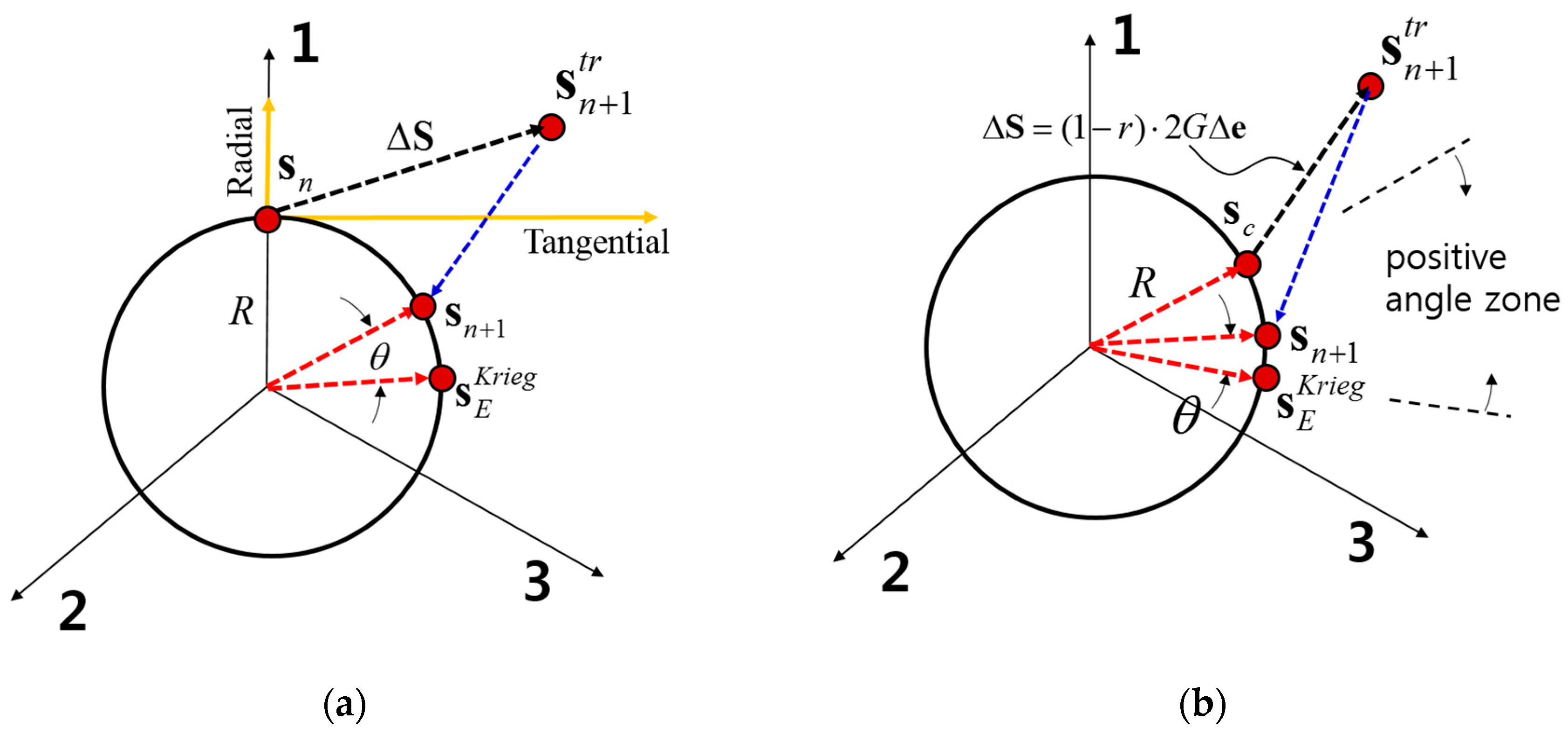
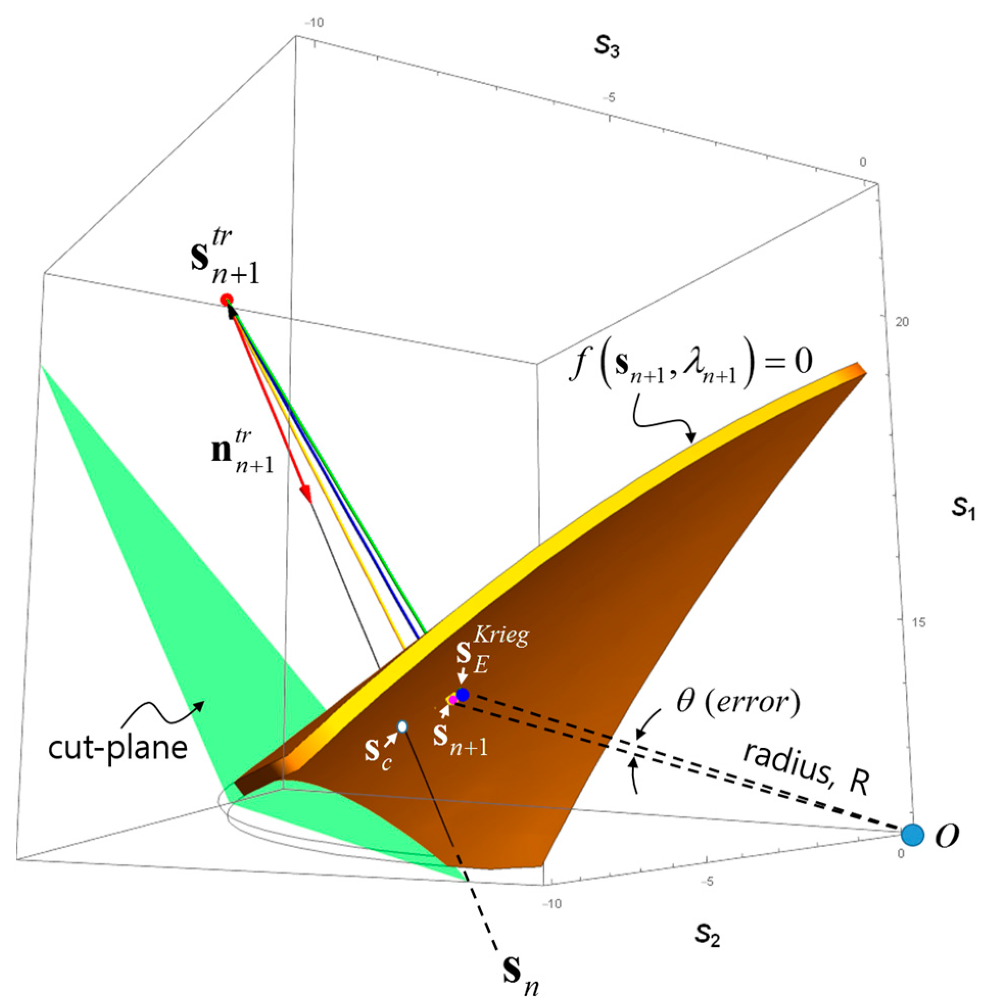
Figure 3a is the specific case which the current stress state resides on the yield surface. Figure 3b is the general case which the current stress state resides inside the yield surface. This means that one needs to calculate the contact stress, when cross through the yield surface. The unknown stress determination using the radial return method in the three-dimensional deviatoric space is shown in Figure 4.
Krieg et al. [2] evaluated the exact stress state at in the perfectly plastic model. In their pioneering work, they compared the three techniques to correct the trial stress: (a) the tangent stiffness–radial return method, (b) the secant stiffness method, and (c) the radial return method. The errors between the exact stress and the stress determined by the radial return method with different values were plotted in the form of an iso-error map, as shown in Figure 5. The errors were plotted in terms of the angle, between and as illustrated in Figure 3b. The error, is defined by Krieg et al. [2] as . R is the radius of deviatoric principal stress plane as shown in Figure 3. In this case, R is the yield strength, or . If lies between and , then the error, becomes positive. is the contact stress when elastic prediction process over a time span such that the yield surface is reached. For the monotonic loading with an arbitrary deviatoric stress increment, between first quadrant of the radial and tangential coordinates in the Figure 3a, the strain rate, was controlled up to five times R of for both the radial and tangential direction. The stress increment, for marching toward the trial stress state, is simply scaled in terms of the reference value, radius R. This is for the purpose of evaluating the solution accuracies due to a different location of elastic predictor in the first quadrant of radial and tangential coordinates. Figure 5 shows various iso-error maps for the linear method. The accuracy improves when , known as the radial return method. The material properties used were E = 210 GPa, = 0.3 and = 900 MPa used. Figure 6 shows the two parallel solution algorithms for finite element analysis: the rate format and the incremental format. The two formulations are equivalent when the material is in the plastic state at and the strain increment, is parallel to the current known deviatoric stress state, . Of course, when the time increment is very small, these two requirements are satisfied.
4. Accuracy of Quadratic Midpoint Integration Method
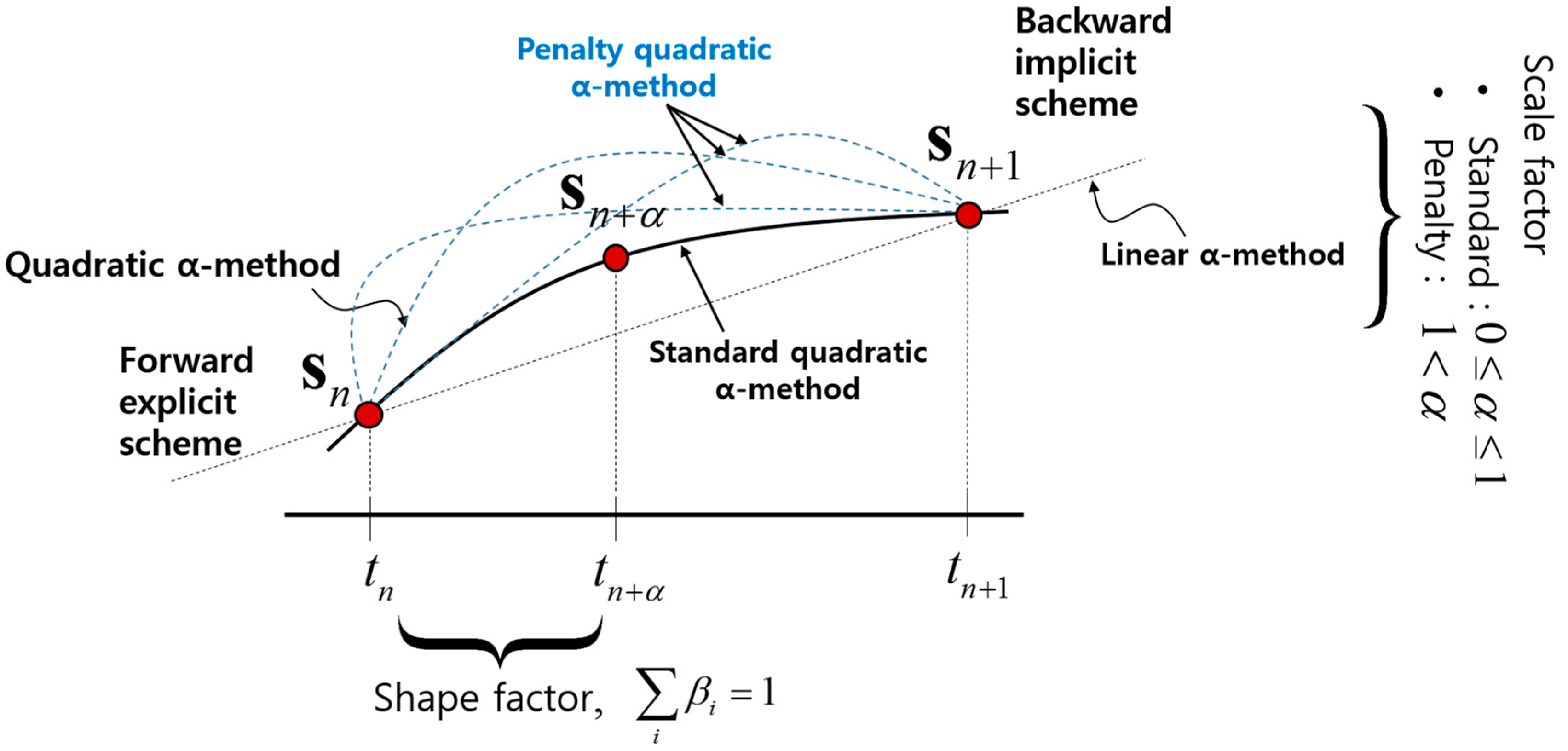
A simple expansion of the linear -method as discussed in the previous section was proposed by Shim [7]. A midpoint time, , bounded by the starting time, , and the arrival time, were added. These three interpolation points allow manipulation of the quadratic midpoint time integration by incorporating the Lagrangian interpolation function, as depicted in Equations (19) and (20). This typical sum of time interval-deviatoric stress products consists of , . k is a number of interpolation point. In our case, .
Using this polynomial expansion, one can express the plastic strain increment, , where . For instance, , , , and , when . The summation of is equal to unity. Thus, is the scale factor and is the shape factor as illustrated in Figure 7. Since the backward implicit scheme, in the linear method shows the best performance in a solution accuracy and a computation time. In this quadratic method, we tried to explore a penalty scale factor that is higher than 1. Although this approach can be seen in the non-logical sense at a glance, it is worthwhile to examine its performance for both solution accuracy and computation time. The accuracies of the quadratic integration methods are plotted in Figure 8. When = 1 and , the method is identical to the backward implicit scheme in the linear -method. In addition, when = 1/2 and , the central difference method is yielded. Thus, as long as , the quadratic integration method coincides with the linear -method. Figure 8b–f shows the results with a range of values and indicates a violation of the interval, . Interestingly, the solution errors compared to Krieg’s exact solution decrease as increases. Figure 8a shows the entire negative solution error in the radial-tangential stress increment domain. However, as increases up to 3, the solution error becomes split into negative and positive components, and its deviation from the zero error iso-line is reduced, as shown in Figure 8b,c, compared to the backward implicit scheme in Figure 8a. In addition, the level of absolute error is reduced in the penalty method. However, when , the negative error diminishes gradually and the positive error prevails, especially in the narrow range of tangential stress increments within . This implies that if is greater than 1, then the positive error within is increased significantly. This will lose solution accuracy significantly. On the other hand, the relatively large stress increment of gives a more accurate estimation compared with that obtained using the standard backward Euler method. This might be helpful for relatively long time steps. In Figure 9, the effects of a range of values of on the solution error were investigated, with a fixed value of . Better solution accuracies were found in Figure 9c,e. The similarity between these two cases arises from the higher weight for as in the backward Euler approach. Hence, the influence of the quadratic time integration method spreads the solution error into the positive and negative ranges, while the relative error deviation is similar from the perspective of solution accuracy. Nevertheless, for the case of a large stress increment, the solution error would decay much faster than in the linear -method. This differs from the results reported by Shim [7]. An iterative solution algorithm for implementing this quadratic time integration the finite element programming is presented in Figure 10. By altering the trial stress in terms of , , one can find under the assumption that so that can be defined as , and the constrained equation in the step at is finally determined by as . K is the bulk modulus.
5. Implementation for Quadratic α Method
The Matlab-based finite element program developed by Ballani [13] was used as a base program for implementing the quadratic method in the stress integration module and associated dependencies. The single-step midpoint methods (SMPTs) applied a generalized midpoint rule for integration of the differential equations of the system. These stress integration schemes were performed once per time interval. The difference between SMPT1 and SMPT2 is the choice of consistency condition at time interval, or . As we introduced the scale factor, and the shape factor, earlier, one can implement the quadratic SMPT1 and SMPT2 as shown in Figure 10. A Newton–Rapson iterative solution technique was used to compute the plastic consistency parameter, . To calculate the consistent tangent moduli, in both the quadratic SMPT1 and SMPT2, the formulations of Equations (21)–(26) were used.
For the quadratic SMPT 1:
where, is a rank-four tensor, is a fourth-order identity tensor and the values of are defined as follows.
Finally, we get
For the quadratic SMPT 2:
Two scale factors were applied to examine the speed of convergence of the calculation of the plastic consistency parameter: the standard method and the so-called penalty method, as shown in Figure 10. The penalty means that if is greater than 1, then the interpolation function layout will be skewed from standard quadratic method as much as the value. Different shape factors were introduced as a weighting method, but the sum of the three components does not necessarily unite as shown in Figure 11.
6. 2D Metal Panel Problem with Slit-Like Defect
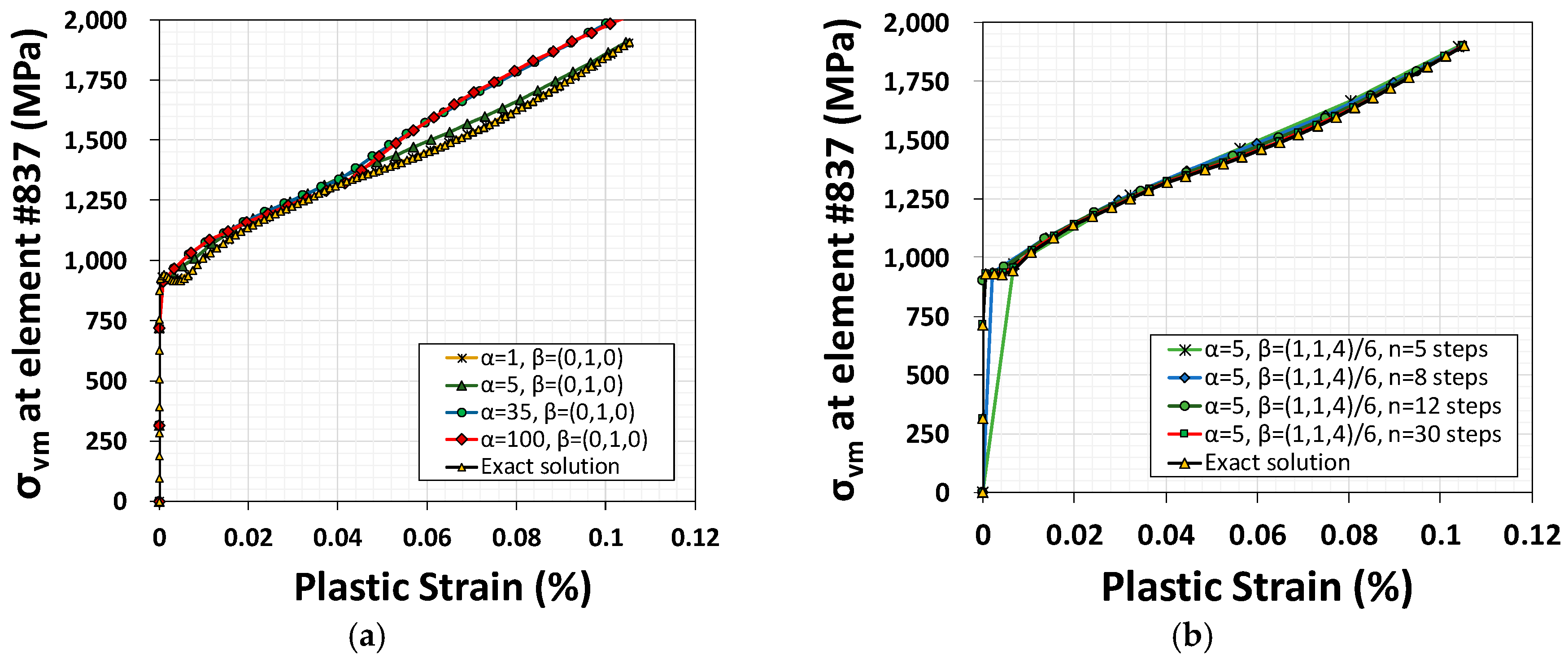
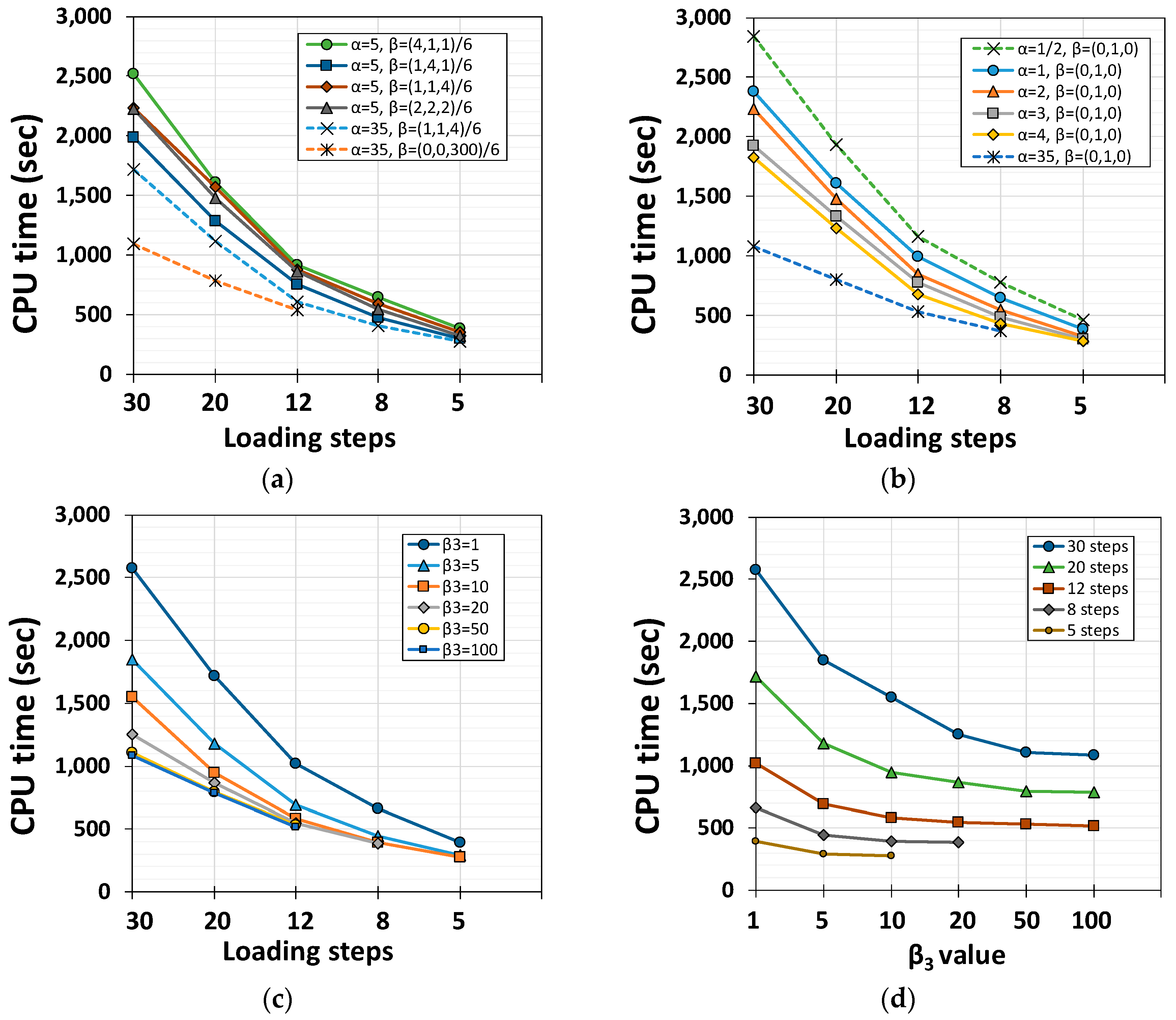
A 1 × 1 mm steel plate with a 0.25 mm slit-like defect in the center was discretized using the Delaunay triangulation scheme with a two-dimensional mesh generator (Persson and Strang, [14]), as shown in Figure 12a,b. A total of 1423 nodes and 2606 CST triangular elements were used. A Matlab based finite element program [13] was used and modified to implement the quadratic -method as discussed in the previous section. An Intel Xeon 2.0 GHz processor was used. The material properties were E = 210 GPa, = 0.3, = 900 MPa. Displacement load control was applied vertically in the upper face of the squared domain up to 0.01 mm for uniform stretching. A single element, #837, in the vicinity of the slit was monitored for von Mises stress during plastification, as shown in Figure 12a. The von Mises stress contour at the final stage of loading is plotted in Figure 12c. The quadratic time integration combinations of discussed in Section 4 were implemented into the finite element program. The convergence performance and accuracy of the solution were compared with the exact solution of the uniform stretching test. The exact solution was assumed from the result of a case with 100 loading steps using the radial return mapping scheme without iteration (rate format by Simo et al. [4,5]), 30, 12, 8, and 5 loading steps were applied for the investigation. Above 30 loading steps, the accuracy of solution should not differ significantly; however, backward Euler method provided a faster convergence rate from all combination of in the quadratic time integration schemes. As discussed earlier, a smaller stress increment produced more severe positive solution errors mainly localized in the narrow region of the small tangential stress increment. For this reason, the backward Euler method in the linear -method still showed better performance. However, for large increments of stress such as the loading step (30, 12, 8 and 5 steps), the backward Euler method lost its stability under the limit of 300 iterations for seeking global Newton–Rapson loops. In contrast, the quadratic time integration scheme with 30, 12, 8 and 5 loading steps showed a stable solution. Table 1 shows that the elapsed computation time and the iteration numbers for each loading step. Figure 13 shows the cross-plots for computational efficiency of the monitored element stress with different time integration schemes. The penalty value reduces the computation time significantly, as shown in Table 1 and Figure 13. However, this leads to a loss in solution accuracy, as shown in Figure 14a. When the shape factor was set to {0,1,0} while the value was varied from 1 to 100, the accuracy of the solution drifted in comparison to the solution from the backward Euler method at 100 time steps (exact solution). Figure 14b shows that light penalty values such as = 5, with a shape factor of {1,1,4}/6 yield more time-efficient results without losing solution accuracy. A comparison of computation time efficiencies between quadratic SMPT1 and SMPT2 is also given in Table 1; the quadratic SMPT2 scheme had a slightly higher efficiency.
7. Conclusions
The quadratic variants of the generalized midpoint rule and return map algorithm for the J2 von Mises metal plasticity model are examined for the accuracy of deviatoric stress integration of the constitutive equation. Based on the Lagrangian interpolation expansion for the linear method, the scale factor and shape factor were introduced to a quadratic integration rule for assuming a returning directional tensor from a trial stress onto the final yield surface. As the perfectly plastic model is the only case where the analytical solution is possible, solution accuracies can be compared with those of the exact solutions with the aid of an iso-error map. Since the standard scale factor ranges from 0 to 1, which is similar to the linear -method, the penalty scale factors greater than 1 were mainly explored to examine the solution accuracies and computational efficiency. A higher value of scale factor above five shows a better computational efficiency but a decreased solution accuracy, especially in the higher plastification zone. A well-balanced scale factor for both computational efficiency and solution accuracy was found to be between one and five. The trade-off scale factor was proposed to be five. The proper shape factor was also proposed to {1,1,4}/6 among the different combinations of weight distribution over a time interval. Since the backward implicit scheme, in the linear method shows the best performance in terms of solution accuracy and a computation time. In this quadratic -method, we tried to explore a penalty scale factor that is higher than 1. Although this approach can be seen in the non-logical sense at a glance, it shows better results in either solution accuracy or computation time. A smaller stress increment produced more severe positive solution errors mainly localized in the narrow region of the small tangential stress increment. For this reason, the backward Euler method in the linear -method still showed better performance. However, for large increments of stress such as the loading step (30, 12, 8 and 5 steps), the backward Euler method lost its stability under the limit of 300 iterations for seeking global Newton–Rapson loops. In contrast, the quadratic time integration scheme with 30, 12, 8 and 5 loading steps showed a stable solution. In addition, the quadratic SMPT2 scheme had a slightly higher efficiency compared to SMPT1.
Acknowledgments
The first author wishes to thank Woo Kim, who introduced him to the field of structural engineering and mechanics in the Civil Engineering Department of Chonnam National University. This paper is dedicated to Woo Kim on the occasion of his retirement.
Author Contributions
Inkyu Rhee performed, analyzed the analysis and wrote the paper. Woo Kim contributed the idea of the paper and corrections to the paper.
Conflicts of Interest
The authors declare no conflict of interest.
References
- Rice, J.R.; Tracey, D.M. Computational fracture mechanics. In Numerical and Computer Methods in Structural Mechanics; Academic Press, Inc.: New York, NY, USA, 1973; pp. 585–623. [Google Scholar]
- Krieg, R.D.; Krieg, D.B. Accuracies of numerical solution methods for the elastic-perfectly plastic model. Trans. ASME 1977, 99, 510–515. [Google Scholar] [CrossRef]
- Ortiz, M.; Popov, E.P. Accuracy and stability of integration algorithms for elastoplastic constitutive relations. Int. J. Numer. Methods Eng. 1985, 21, 1561–1576. [Google Scholar] [CrossRef]
- Simo, J.C.; Taylor, R.L. A return mapping algorithm for plane stress elastoplasticity. Int. J. Numer. Methods Eng. 1986, 22, 649–670. [Google Scholar] [CrossRef]
- Simo, J.C.; Hughes, T.J.R. Computational Inelasticity; Springer: Berlin, Germany, 1998; pp. 1–392. ISBN 0-387-97520-9. [Google Scholar]
- Willam, K.J. Computational Mechanics of Solids and Structures (Class Note); University of Colorado: Boulder, CO, USA, 2002. [Google Scholar]
- Shim, H. Higher-order α-method in computational plasticity. KSCE J. Civ. Eng. 2005, 9, 255–259. [Google Scholar] [CrossRef]
- Artioli, E.; Auricchio, F.; Beirão da Veiga, L. Generalized midpoint integration algorithms for J2 plasticity with linear hardening. Int. J. Numer. Methods Eng. 2007, 72, 422–463. [Google Scholar] [CrossRef]
- Jahanshahi, M. Second order integration algorithms for J2 plasticity with generalized isotropic/kinematic hardening. Asian J. Civ. Eng. 2012, 13, 203–232. [Google Scholar]
- Tresca, H. Mémoire sur l’écoulement des corps solides soumis à de fortes pressions. C. R. Hebd. Séances Acad. Sci. 1864, 59, 754–758. [Google Scholar]
- Von Mises, R. Mechanik der festen Körper im plastisch-deformablen Zustand, Nachrichten von der Gesellschaft der Wissenschaften zu Göttingen. Math.-Phys. Kl. 1913, 1, 582–592. [Google Scholar]
- Boerja, R.I. Plasticity: Modeling & Computation; Springer: Berlin, Germany, 2013; pp. 31–40. [Google Scholar]
- Ballani, J. Three Solution Methods for Perfect Plasticity. 2008. Available online: http://m2matlabdb.ma.tum.de (accessed on 1 August 2017).
- Persson, P.-O.; Strang, G. A simple mesh generator in Matlab. SIAM Rev. 2004, 46, 329–345. [Google Scholar] [CrossRef]
Figure 1.
Failure surface of J2 plasticity: (a) principal stress space, (b) deviatoric stress space.
Figure 1.
Failure surface of J2 plasticity: (a) principal stress space, (b) deviatoric stress space.
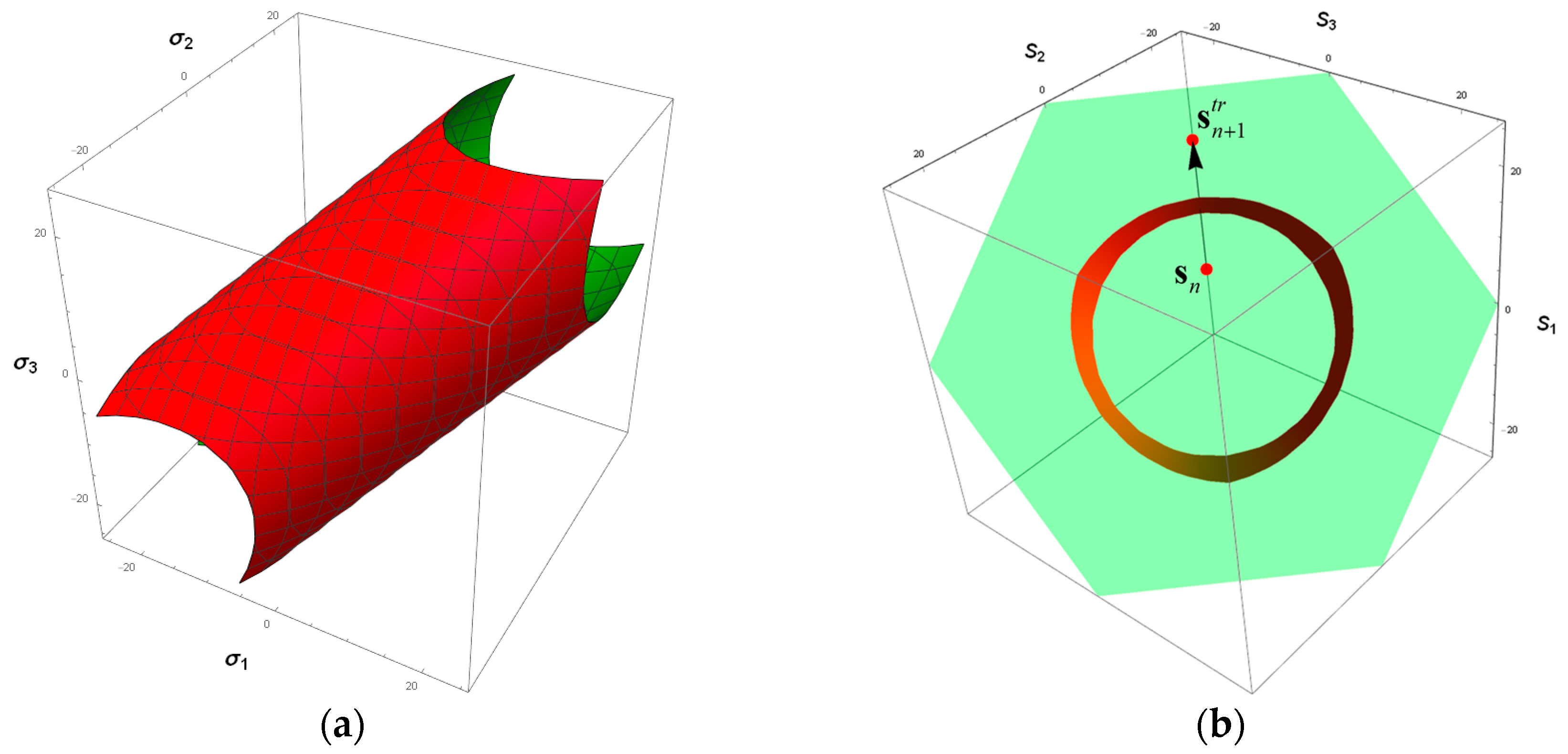
Figure 2.
Time linearization for defining the midpoint deviatoric stress.
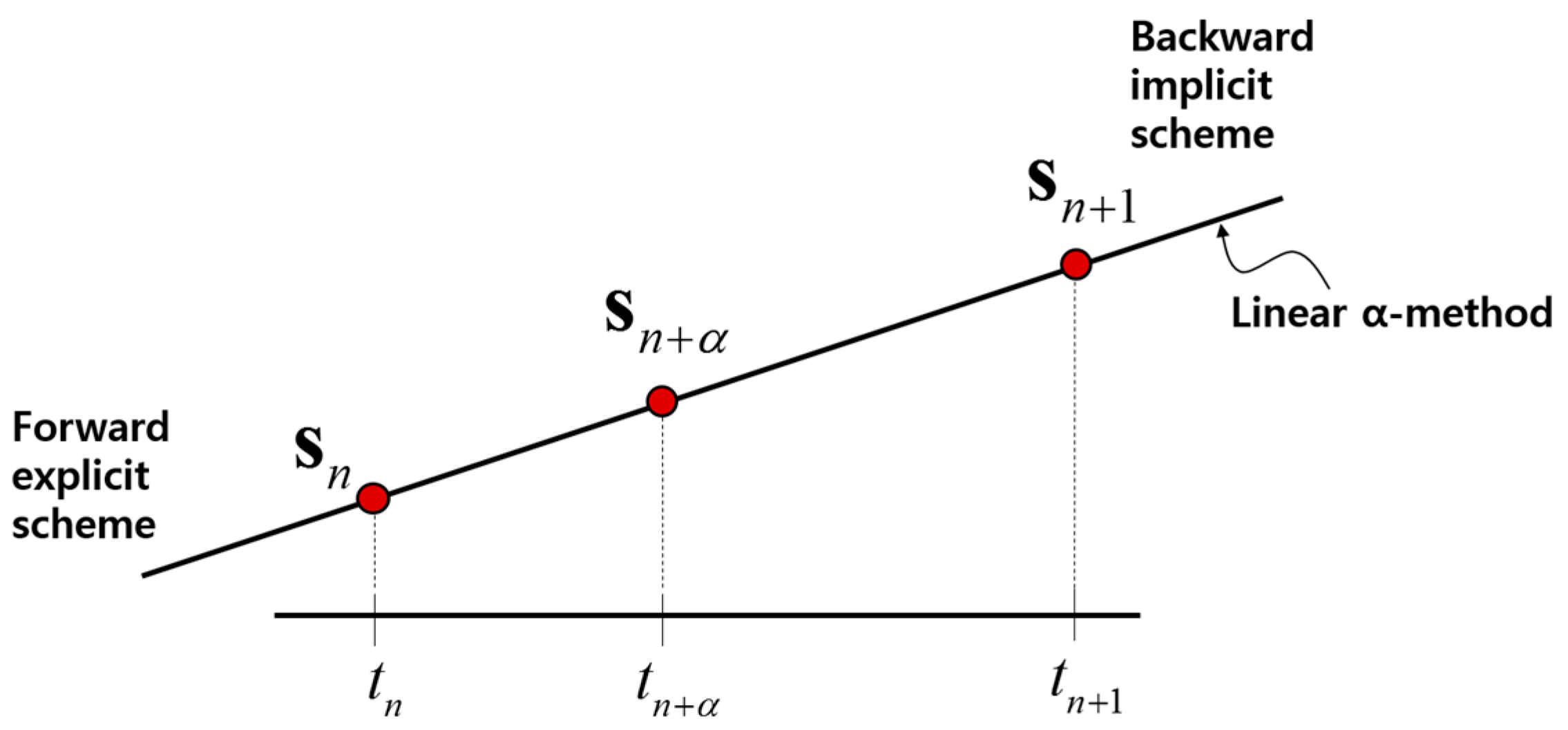
Figure 3.
Deviatoric principal stress plane: (a) radial and tangential coordinates at the contact stress, , and (b) positive angular error shown between computed and exact stress is identified at each trial stress state, . is the final stress which was corrected by the radial return method. Note: r is the distance proportion between and over the time interval.

Figure 4.
Radial return algorithm: trial stress over the yield surface and corrected final stress onto the yield surface: calculation and visualization using Mathematica.
Figure 4.
Radial return algorithm: trial stress over the yield surface and corrected final stress onto the yield surface: calculation and visualization using Mathematica.

Figure 5.
Validation of the linear α-method: (a) central difference, ; (b) skewed difference,; and (c) backward Euler integration, .
Figure 5.
Validation of the linear α-method: (a) central difference, ; (b) skewed difference,; and (c) backward Euler integration, .
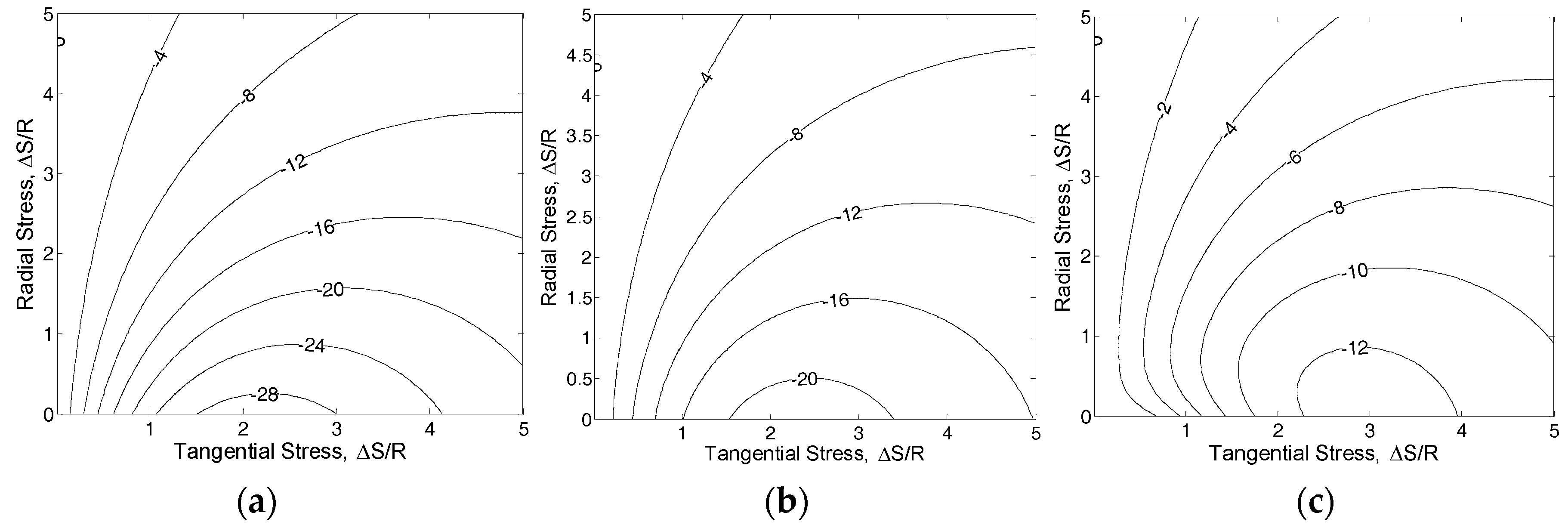
Figure 6.
Solution algorithm for radial return method and linear generalized trapezoidal method in J2 plasticity (rearranged and cast by the author from Simo et al. [4,5]), Note: K is the bulk modulus and k is the iteration number.
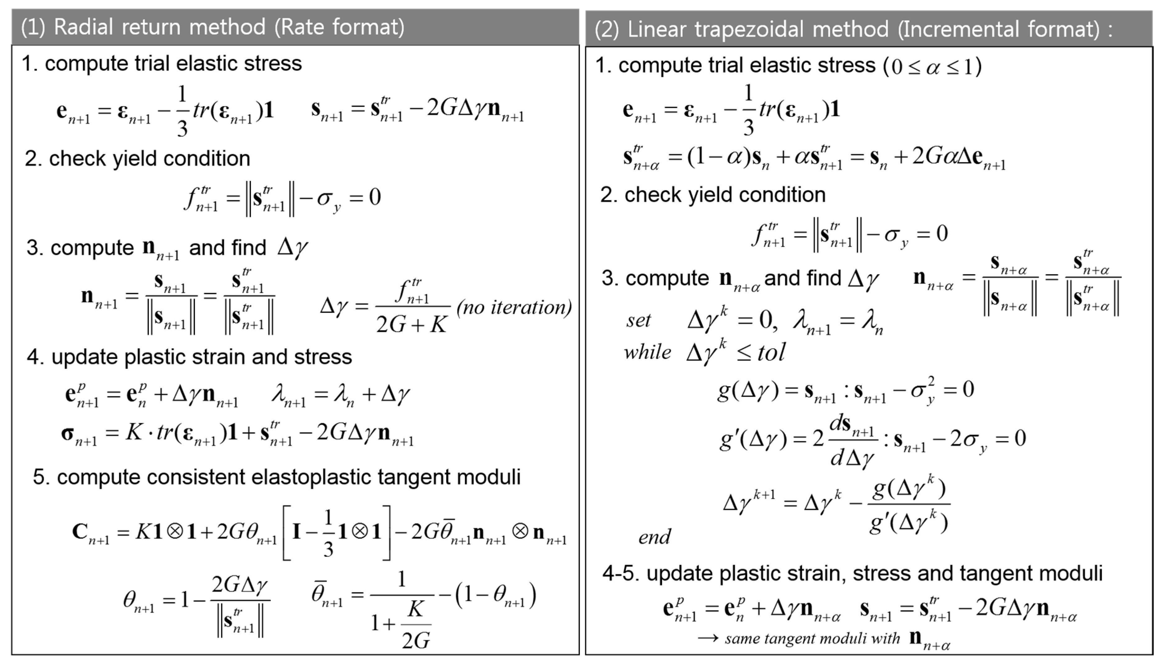
Figure 7.
Quadratic generalized trapezoidal method in J2 plasticity.

Figure 8.
Validation for quadratic α-method: midpoint and backward Euler integration.
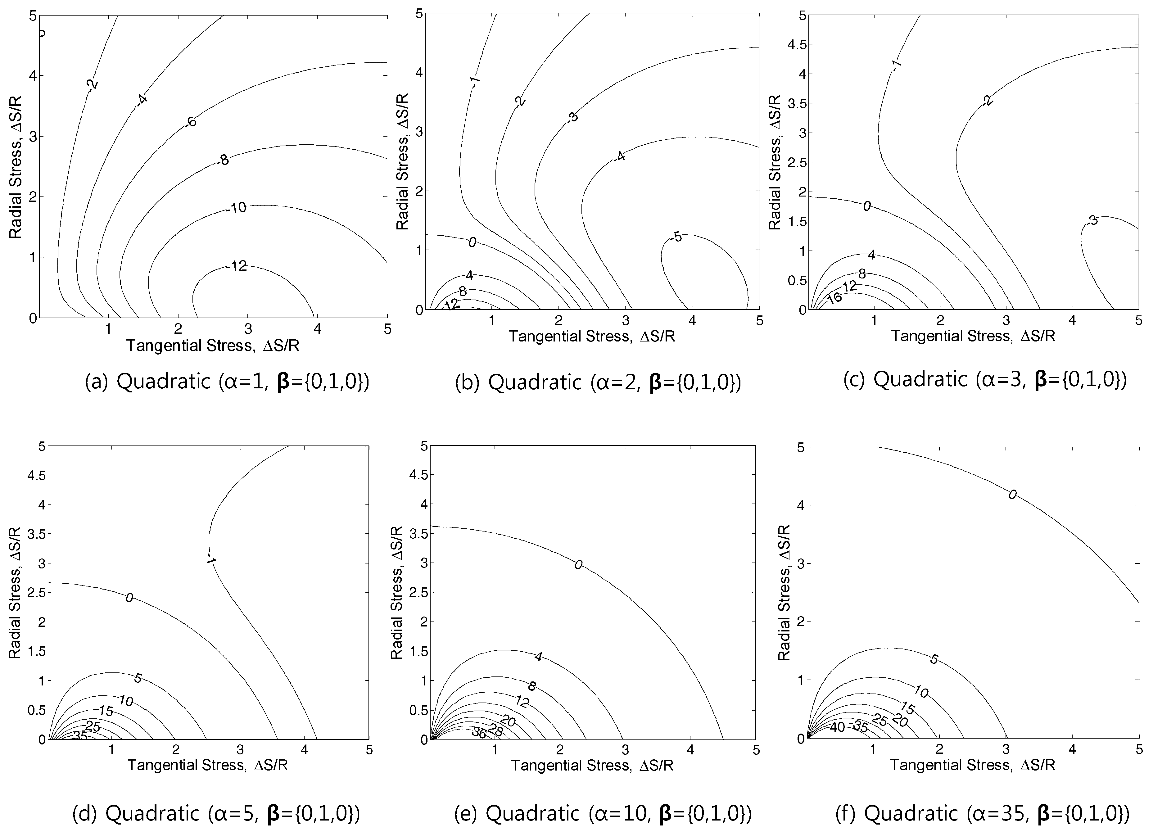
Figure 9.
Error leakage in the vicinity of small increment less than .

Figure 10.
Solution algorithm for quadratic generalized trapezoidal method in J2 plasticity (by rearranged and casted by the author from Simo et al. [4,5]).
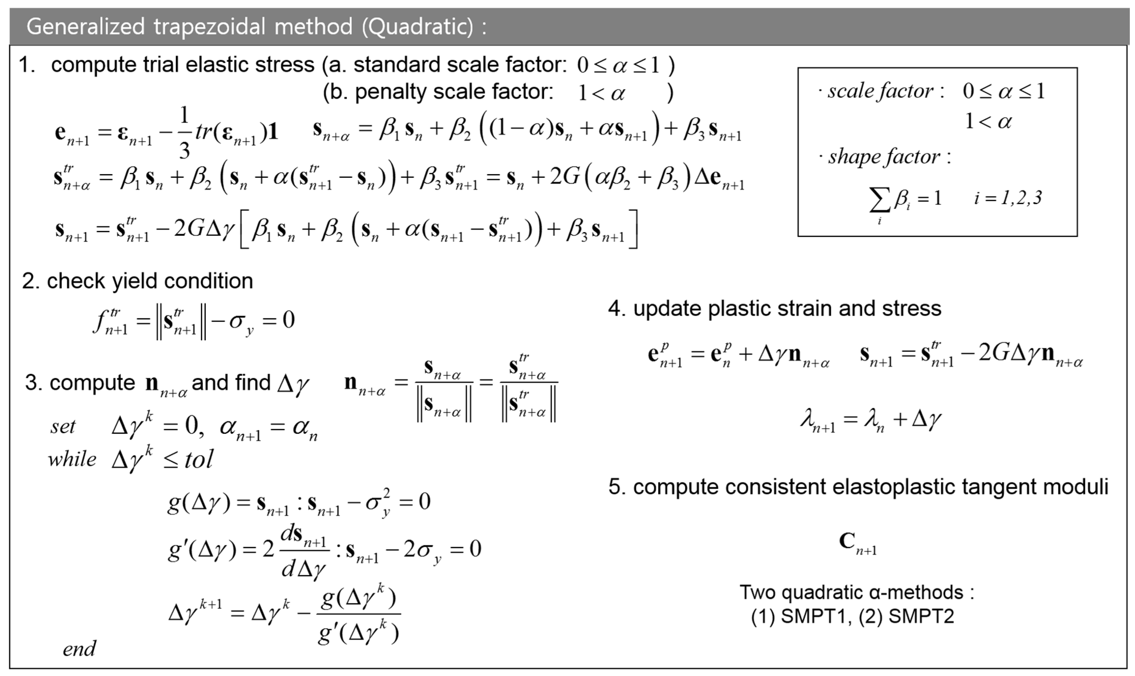
Figure 11.
Quadratic single-step midpoint methods (SMPT1 and SMPT2): standard α-method and penalty α-method.
Figure 11.
Quadratic single-step midpoint methods (SMPT1 and SMPT2): standard α-method and penalty α-method.
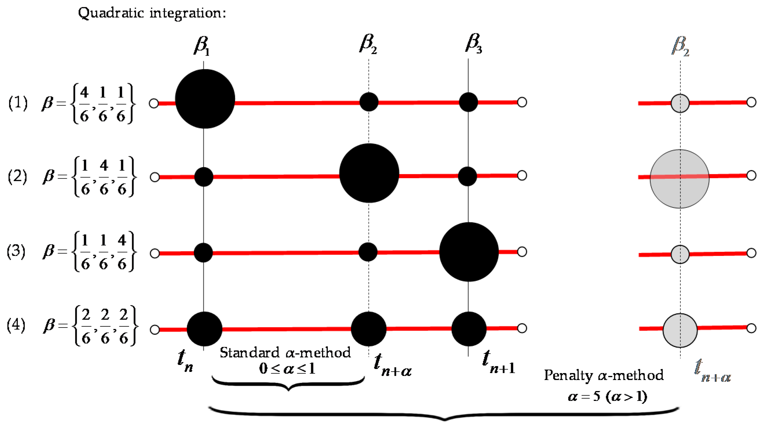
Figure 12.
Two-dimensional metal panel problem with slit-like defect: (a) elements monitored, (b) finite element mesh layout and (c) von Mises stress contour plot.
Figure 12.
Two-dimensional metal panel problem with slit-like defect: (a) elements monitored, (b) finite element mesh layout and (c) von Mises stress contour plot.
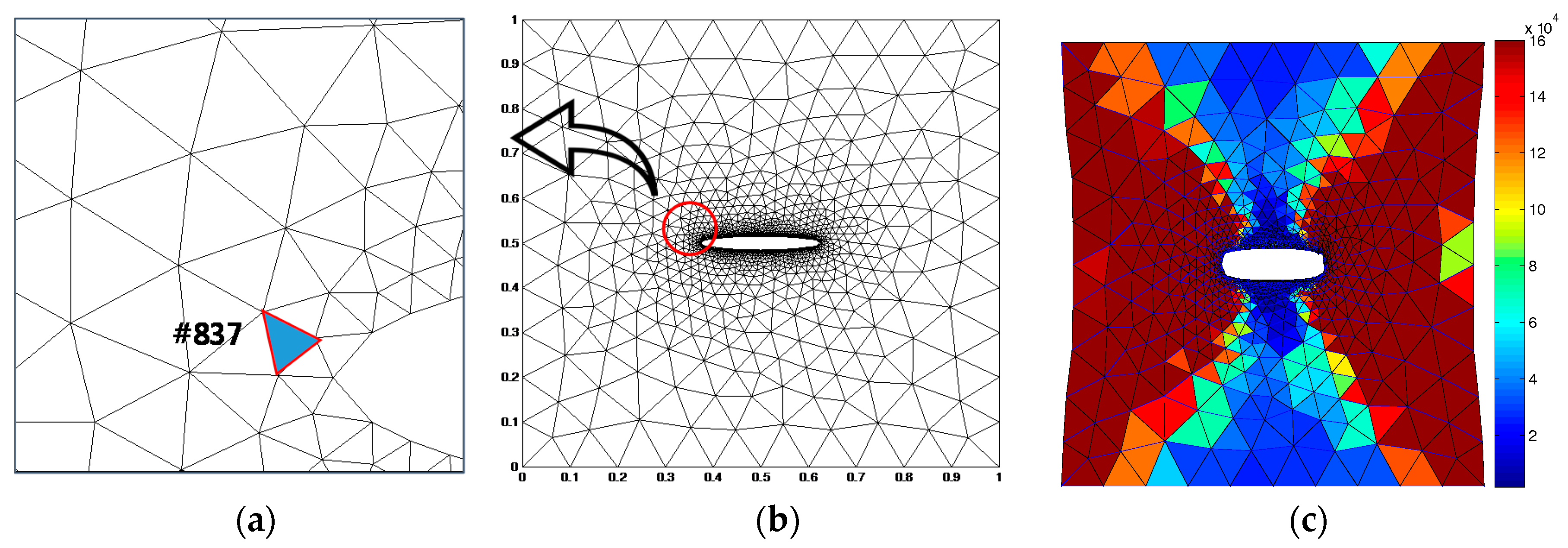
Figure 13.
Computational efficiency of Quadratic SMPT1 using the standard α-method and penalty α-method : the influences of different (a) weights, (b) values, (c) which is the third component of, and (d) time intervals.
Figure 13.
Computational efficiency of Quadratic SMPT1 using the standard α-method and penalty α-method : the influences of different (a) weights, (b) values, (c) which is the third component of, and (d) time intervals.

Figure 14.
Validation for quadratic α-method using von Mises stress at the element #837: (a) varies from 1 to 100, while is kept constant as {0,1,0}, (b) time steps varies from 5 to 30, while and are kept constants as 5 and {1,1,4}/6, respectively.
Figure 14.
Validation for quadratic α-method using von Mises stress at the element #837: (a) varies from 1 to 100, while is kept constant as {0,1,0}, (b) time steps varies from 5 to 30, while and are kept constants as 5 and {1,1,4}/6, respectively.

Table 1.
Computation (CPU) time for different time integration schemes (unit: second (s)).
| Time Integration Schemes | 30 Steps | 12 Steps | 8 Steps | 5 Steps | ||
|---|---|---|---|---|---|---|
| Quadratic -SMPT1 | All | 2578.4 | 1019.6 | 660.8 | 392.1 | |
| 2377.6 | 998.3 | 648.2 | 385.4 | |||
| 2235.1 | 846.8 | 549.3 | 323.2 | |||
| 1925.9 | 781.5 | 488.2 | 305.3 | |||
| 1823.1 | 678.5 | 436.0 | 285.0 | |||
| 1533.0 | 575.7 | diverged 1 | 263.1 | |||
| 1082.1 | 530.3 | 367.3 | diverged 1 | |||
| 1984.4 | 754.3 | 479.4 | 303.2 | |||
| 2521.9 | 918.4 | 651.5 | 387.0 | |||
| 2234.2 | 878.9 | 591.2 | 358.3 | |||
| 2228.9 | 860.5 | 549.2 | 326.4 | |||
| 1717.3 | 606.0 | 411.4 | 276.7 | |||
| 1092.7 | 542.3 | diverged 1 | diverged 1 | |||
| Quadratic -SMPT2 | 2523.1 | 992.8 | 640.3 | 378.1 | ||
| 2256.8 | 868.4 | 552.4 | 319.2 | |||
| 2055.7 | 753.2 | 486.2 | 303.0 | |||
| 1833.7 | 682.1 | 422.1 | 266.7 | |||
| 1541.8 | 543.1 | diverged 1 | diverged 1 | |||
| 1137.9 | diverged 1 | diverged 1 | diverged 1 | |||
| 2011.6 | 693.8 | 476.6 | 297.4 | |||
| 2540.2 | 990.2 | 638.5 | 378.7 | |||
| 2206.7 | 884.0 | 594.2 | 352.0 | |||
| 2285.7 | 858.0 | 552.0 | 319.2 | |||
| 1728.6 | 610.4 | diverged 1 | 270.4 | |||
| diverged 1 | diverged 1 | diverged 1 | diverged 1 | |||
1 Solution had been exceeded 300 iterations for global Newton–Raphson iteration loop.
© 2018 by the authors. Licensee MDPI, Basel, Switzerland. This article is an open access article distributed under the terms and conditions of the Creative Commons Attribution (CC BY) license (http://creativecommons.org/licenses/by/4.0/).
Share and Cite
MDPI and ACS Style
Rhee, I.; Kim, W. Quadratic Midpoint Integration Method for J2 Metal Plasticity. Metals 2018, 8, 66. https://doi.org/10.3390/met8010066
AMA Style
Rhee I, Kim W. Quadratic Midpoint Integration Method for J2 Metal Plasticity. Metals. 2018; 8(1):66. https://doi.org/10.3390/met8010066
Chicago/Turabian StyleRhee, Inkyu, and Woo Kim. 2018. "Quadratic Midpoint Integration Method for J2 Metal Plasticity" Metals 8, no. 1: 66. https://doi.org/10.3390/met8010066
Note that from the first issue of 2016, this journal uses article numbers instead of page numbers. See further details here.