Numerical Study on Flow, Temperature, and Concentration Distribution Features of Combined Gas and Bottom-Electromagnetic Stirring in a Ladle


1
Key Laboratory of Electromagnetic Processing of Materials (Ministry of Education), Northeastern University, No. 3-11, Wen hua Road, Shenyang 110004, China
2
School of Metallurgy, Northeastern University, No. 3-11, Wen hua Road, Shenyang 110004, China
*
Author to whom correspondence should be addressed.
Metals 2018, 8(1), 76; https://doi.org/10.3390/met8010076
Submission received: 24 October 2017
/
Revised: 2 January 2018
/
Accepted: 15 January 2018
/
Published: 19 January 2018
Abstract
:A novel method of combined argon gas stirring and bottom-rotating electromagnetic stirring in a ladle refining process is presented in this report. A three-dimensional numerical model was adopted to investigate its effect on improving flow field, eliminating temperature stratification, and homogenizing concentration distribution. The results show that the electromagnetic force has a tendency to spiral by spinning clockwise on the horizontal section and straight up along the vertical section, respectively. When the electromagnetic force is applied to the gas-liquid two phase flow, the gas-liquid plume is shifted and the gas-liquid two phase region is extended. The rotated flow driven by the electromagnetic force promotes the scatter of bubbles. The temperature stratification tends to be alleviated due to the effect of heat compensation and the improved flow. The temperature stratification tends to disappear when the current reaches 1200 A. The improved flow field has a positive influence on decreasing concentration stratification and shortening the mixing time when the combined method is imposed. However, the alloy depositing site needs to be optimized according to the whole circulatory flow and the region of bubbles to escape.
1. Introduction
Ladle metallurgy plays an important role in modern steelmaking processes. Strong turbulent flow in the ladle beneficially enhances the chemical reaction rate, homogenizes the chemical composition, removes non-metallic inclusions, and eliminates temperature stratification. In addition, enhancing turbulence at the slag/steel interface is required to achieve a desirable desulphurization result [1]. Argon gas stirring (AGS) and electromagnetic stirring (EMS) are the two dominant methods in the ladle refining process [2,3,4,5,6].
A gas-liquid plume is essential for dehydrogenation and denitrogenation in ladle refining [7]. However, a bare metal surface region, called the “open-eye”, will be observable when the velocity of argon bubbles is large enough and the slag layer is relatively thin. The open-eye region increases the amount of oxygen dissolvable in molten steel, therefore resulting in re-oxidation and slag entrapment [8,9]. In addition, the heat loss will escalate due to the argon gas having a comparatively lower temperature than the molten steel. The mixing effect of AGS with a single central plug is not enough to eliminate the temperature and concentration stratification, and the dead zone easily emerges in the region of the ladle bottom far away from the plug, resulting in temperature and concentration stratification. Although there are a few reports aiming to improve the flow field and reduce the dead zone by changing the plug configurations, such as eccentric plug [10,11,12] and by adoption of the dual-plugs with different placement [13,14,15,16], the flow field is not fully stirred at the normal argon blowing rate. The method of improving flow field by increasing argon blowing rate is inadvisable considering the phenomena of re-oxidation and slag entrapment near the extended open eye. EMS can generate a vigorous stirring in melt by keeping the whole melt surface covered in slag layer. The strength of EMS can be controlled accurately, which leads to high reproducibility and operational flexibility. The stirring direction of EMS can be changed easily. The Joule heat produced by alternating electromagnetic field can partly compensate the heat loss during the refining process. Therefore, the combination of EMS and AGS can utilize the advantages of both mixing methods and improve the performance of a ladle furnace. Chung [17] studied the three-dimensional turbulent fluid flow in the ASEA-SKF ladle with the method of side-traveling EMS, AGS, and that of combined stirring. Their results show that side-traveling EMS is superior to AGS for the removal of non-metallic inclusions, however, AGS is more advantageous for a better mixing result. The combined stirring is more effective than each individual stirring method. Sand [18] studied the effect of AGS with side-traveling EMS on the action of gas plume, stirring energy, velocity, and mixing time, and mentioned that there is a significant potential to implement this method in the ladle refining process to shorten the production time and make cleaner steel. Although Chung et al. and Sand et al. have investigated the combined stirring method, the combined stirring method with AGS and bottom-rotating EMS has never been reported.
In the present study, a rotating electromagnetic stirrer was designed, and a novel stirring method combining AGS and bottom-rotating EMS in the ladle refining process was presented. For the purpose of evaluating its effect on improving flow field, eliminating temperature stratification and homogenizing concentration distribution, a three-dimensional Eulerian-Eulerian two phase numerical model was built. In addition, the trajectory of argon bubbles was also analyzed by the Eulerian-Lagrangian approach. Operational parameters including stirring intensity were taken into consideration.
2. Model Descriptions
2.1. Basic Assumptions
In order to simulate the phenomena in a ladle, the following assumptions are made in the formulated models:
- (1)
- The molten steel is an incompressible continuous fluid, and the bubbles are a discrete phase fluid with a constant diameter of 4 mm, the average bubble diameter was evaluated from empirical equation proposed by Davidson and Schuler [19];
- (2)
- The break-up and coalescence of gas bubbles are neglected;
- (3)
- The ladle is filled with molten steel and the effect of the slag layer on the fluid flow is ignored;
- (4)
- The buoyant force and electromagnetic force (EMF) are mainly responsible for the fluid flow and the movement of bubbles;
- (5)
- The effect of temperature on the physical properties is ignored and the parameter of materials is regarded as a constant;
- (6)
- The displacement current is negligible.
2.2. Governing Equations
2.2.1. Eulerian-Eulerian Model
The molten steel and argon gas flow are treated as two different continuous phases interpenetrating and interacting with each other. The EMF is added to the momentum equation as source term to drive molten steel flow. The flow equations for different phase are weighted by their volume fraction and can be described as follows.
For the liquid phase:
and:
For the gas phase:
and:
where α, ρ, t, u, p, and g are the volume fraction, density, time, velocity, pressure, and the gravitational acceleration, respectively. The subscripts l and g denote the liquid and gas phase, respectively. μeff is the effective viscosity. Flg = −Fgl represents the interaction force of the two phases:
The terms on the right hand side of Equation (5) are the drag force, lift force, virtual mass force, turbulent dispersion force, and wall lubrication force, respectively. Here, the drag force, lift force, virtual mass force, and turbulent dispersion force are taken into consideration.
The drag force is calculated according to:
The Schiller Naumann model [20] is employed for the drag force coefficient CD. The db in Equation (6) is the bubble diameter. The Schiller Naumann model may be described as:
where Reb is the bubble Reynolds number and μl is the dynamic viscosity of molten steel.
The lift force [21] in terms of the slip velocity and the curl of the liquid phase velocity is described by:
The present work focuses on the bubbly flow regime of small spherical bubbles, where only a positive lift force coefficient is sufficient, and the constant CL (lift force coefficient) is set to 0.5.
The virtual mass force accounts for relative acceleration and the additional work performed by bubbles in accelerating the liquid surrounding the bubbles. The acceleration of the liquid is taken into account through the virtual mass force, which is given by:
The virtual mass force coefficient CVM is taken to be 0.5 for individual spherical bubble.
The turbulent dispersion force results in the additional dispersion of phases from high volume fraction regions to low volume fraction regions due to turbulent fluctuations. The turbulent dispersion force is given based on Favre Average Drag Model proposed by Burns et al. [22]:
where the turbulent dispersion coefficient CTD = 1.0 and the turbulent Schmidt number σT,l = 0.9 are adopted. The μT,l in Equation (11) is the molten steel turbulence kinetic viscosity.
The total conservation requires:
2.2.2. Turbulent Model
For two-phase turbulent flow, unlike single-phase fluid flow problem, there is no standard turbulent model. However, the standard k-ε turbulence model proposed by Launder and Spalding [23] has been successfully employed to study the two-phase flow in many studies [19,24]. Therefore, this model was adopted in the present research. The effective viscosity in Equations (2) and (4) is formulated as follows:
The turbulent kinetic energy and its energy dissipation rate are calculated from the following equations:
where Gk is the rate of production of turbulent kinetic energy. Other model constants are: Cμ,T = 0.09, Cε1 = 1.44, Cε2 = 1.92, σk = 1.00, and σε = 1.30.
2.2.3. Electromagnetism Model
The mathematical modelling for electromagnetic field analysis is based on the famous Maxwell equations stated below:
and by the constitutive equation:
where E is the electric field intensity, B is the magnetic flux density, H is the magnetic intensity, J is the current density, η is the magnetic permeability, and σ is the electrical conductivity.
The following equation can be deduced by combining Equations (18) and (20)–(22):.
The first term of Equation (23) is the magnetic convection term, and the second is the magnetic diffusion term. The magnetic Reynolds number and the skin depth can be described as:
where L is the characteristic length, ul is the magnitude of flow field characteristic velocity and ω is the angular frequency. At low frequencies, this criterion of judging the influence of the flow velocity on the magnetic field is more restrictive due to the shielding parameter [25], the square of the ratio of the length scales L and δ, and requires that:
In our research, Equation (26) is easily met with the frequency range of 30 Hz to 80 Hz. Therefore, the influence of flow velocity on the magnetic field can be ignored.
The preceding equations can be analyzed in terms of magnetic vector potential A and electric scalar potential φ, which can be described as:
The conductive current density J including both the source and induced components may be obtained by combining Equations (18), (22), (27), and (28):
2.2.4. Energy Transfer Model
The Joule heat generated by alternating electromagnetic field is added to the energy equation as a source term. To obtain a precise prediction of the temperature field of molten steel, the energy equation is applied and may be described as:
where cp is the specific heat capacity at constant pressure, λ is the thermal conductivity and Qv is the source term produced by the alternating electromagnetic field.
2.2.5. Discrete Phase Model
The trajectory of bubbles is also investigated by a Euler-Lagrangian method. The trajectory of bubbles is calculated in each time step according to the buoyancy force, drag force, virtual mass force, turbulent dispersion force, pressure gradient force, and electromagnetic repulsive force [28]. Therefore, the governing equation may be described as:
where FB, Fp, and Fem can be written as:
2.2.6. Species Transport Model
The mixing time in a ladle-combined EMS with AGS is calculated by solving the following species transport equation:
where C is the mass fraction of the species, D0 is molecular dissipation coefficient of the species, and SCt is the turbulent Schmidt number, which is set to 0.7.
3. Geometrical Model and Computational Conditions
3.1. Geometrical Model and Verification of Grid-Independence
Figure 1 shows the schematic view of the geometric model. The ladle is conical shape with a height of 3.732 m. The top and bottom diameters for the ladle are 2.98 m and 2.60 m, respectively. Argon gas is injected through a porous plug with diameter of 118 mm located at the bottom of the ladle. The position of the porous plug is located at half of ladle bottom radius. The electromagnetic stirrer is composed of coils, iron cores, and an insulating base located under the center of ladle bottom, as shown in the figure. A three-phase alternating current with a phase angle difference of 120 degrees is supplied to the coils. The detailed model parameters and computational conditions are given in Table 1.
With regard to the hydrodynamic analysis, error statistics of the computational results for different grid nodes are summarized in Table 2. In the computational domain, the following case was chosen to verify a non-correlation between the number of grid nodes and calculation results. The basic operating parameters are as follows: an argon blowing rate of 600 L·min−1 and a stirring current of 600 A. The influence of the combined method on the behavior of molten steel flow was mainly discussed below, so the computational results of molten steel velocity along with the central axis of ladle were used as the basis for verification. The errors εux, εuy, εuz, and εu relative to the finest mesh case D are estimated (see Table 2, where the exact definition of these quantities is given). ux, uy, uz, and u are the averaged velocity values at the central axis of the ladle. The results show that the velocity errors decrease as the number of cells increased. Therefore, Case B is selected in the present simulation, which ensures good precision at a reasonable computational cost. The time-step of 0.008 s and the convergence criteria of 1 × 10⁻⁴ were used for the computations.
3.2. Computational Method and Boundary Conditions
As for the simulation analysis, the hydrodynamic problem and the electromagnetic problem including the distribution of EMF and Joule heat about the bottom-rotating EMS are individually analyzed using ANSYS Classic software (Version 11.0, ANSYS, Pittsburgh, PA, USA, 2008) and ANSYS CFX software (Version 11.0, ANSYS, Pittsburgh, PA, USA, 2008). Firstly, the electromagnetic analysis is performed and the data including the time-averaged EMF distribution and the Joule heat distribution is derived. Secondly, a transient analysis, including flow field with the time-averaged EMF as the momentum source and temperature field with the Joule heat as the energy source, is performed, lasting for 360 s. Then, a transient concentration field analysis based on the results of the second step is performed. Finally, neglecting the effect of bubbles on the flow field, the trajectory of argon bubbles is also analyzed based on the results of the second step.
For the electromagnetic simulation, an air cube (side length approx. 8 m) around the whole ladle and the electromagnetic stirrer geometry is used to capture a great part of the magnetic field lines closing in the surrounding air. Boundary conditions with zero magnetic vector are applied on the external surfaces of the surrounding air cube, which means the magnetic field intensity is zero on the outside of the simulation region.
For the analysis of fluid flow, a non-slip boundary condition is used at the bottom and side wall with standard “wall functions” in order to capture the steep gradients with reasonable accuracy on a coarse grid. The top surface is modelled as a degassing boundary condition, where dispersed bubbles are permitted to escape, but the fluid is not. The continuous phase may treat the boundary as a free-slip wall and the dispersed fluid phases treat this boundary as an outlet. As for temperature field analysis, the initial temperature of molten steel is set to 1873 K. The specified heat flux density at the ladle wall is 11,702 W·m−2 and 8532 W·m−2 at the ladle bottom. The heat loss on the top surface is ignored.
4. Results and Discussion
4.1. Analysis of Electromagnetic Force
The distribution of EMF on bottom surface (Z = 0 m) and vertical section (Y = 0 m) of the ladle are shown in Figure 2a,b, respectively. Figure 2a shows a clockwise spin of the EMF distribution on the bottom surface, which may drive molten steel in the vicinity of the ladle bottom to rotate and further drive the bulk to rotate due to the shear force. Figure 2b shows at the Y = 0 m section, there is evidence of upward-pointing parabolic EMF distribution, more concentrated in the middle and less on either end of the vertex. The resultant force has an upward and rotational direction and, therefore, may drive molten steel in an upward and rotational motion.
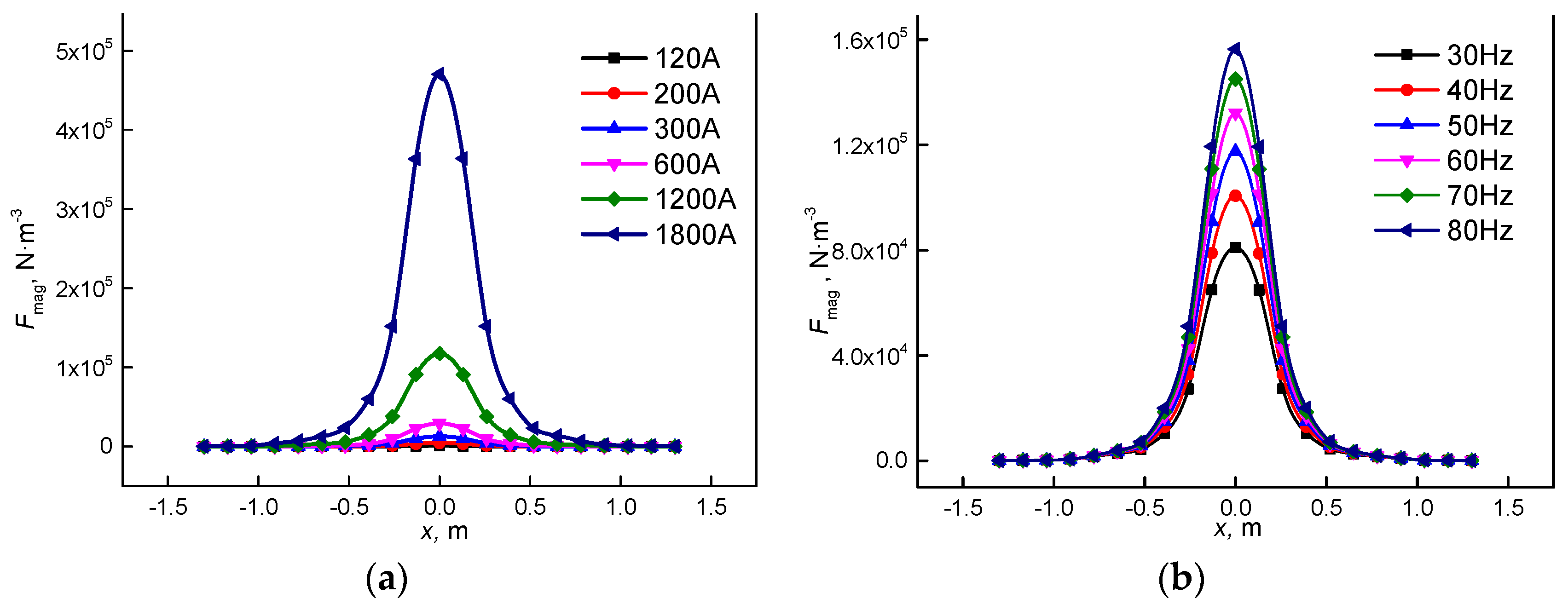
Figure 3 illustrates the magnitude distribution of EMF along the radial direction on the bottom surface with different current intensity and frequency. The distribution characteristics of EMF increase with current intensity and increasing frequency, but the current intensity is most influential on the magnitude of EMF. Due to the skin effect, the penetration depth of EMF is determined by the magnetic field frequency. When the adopted frequency varies from 30 Hz to 80 Hz, the penetration depth is small at about 0.1 m which implies that the adopted frequency range has little effect on the penetration depth.
4.2. Analysis of Flow Field
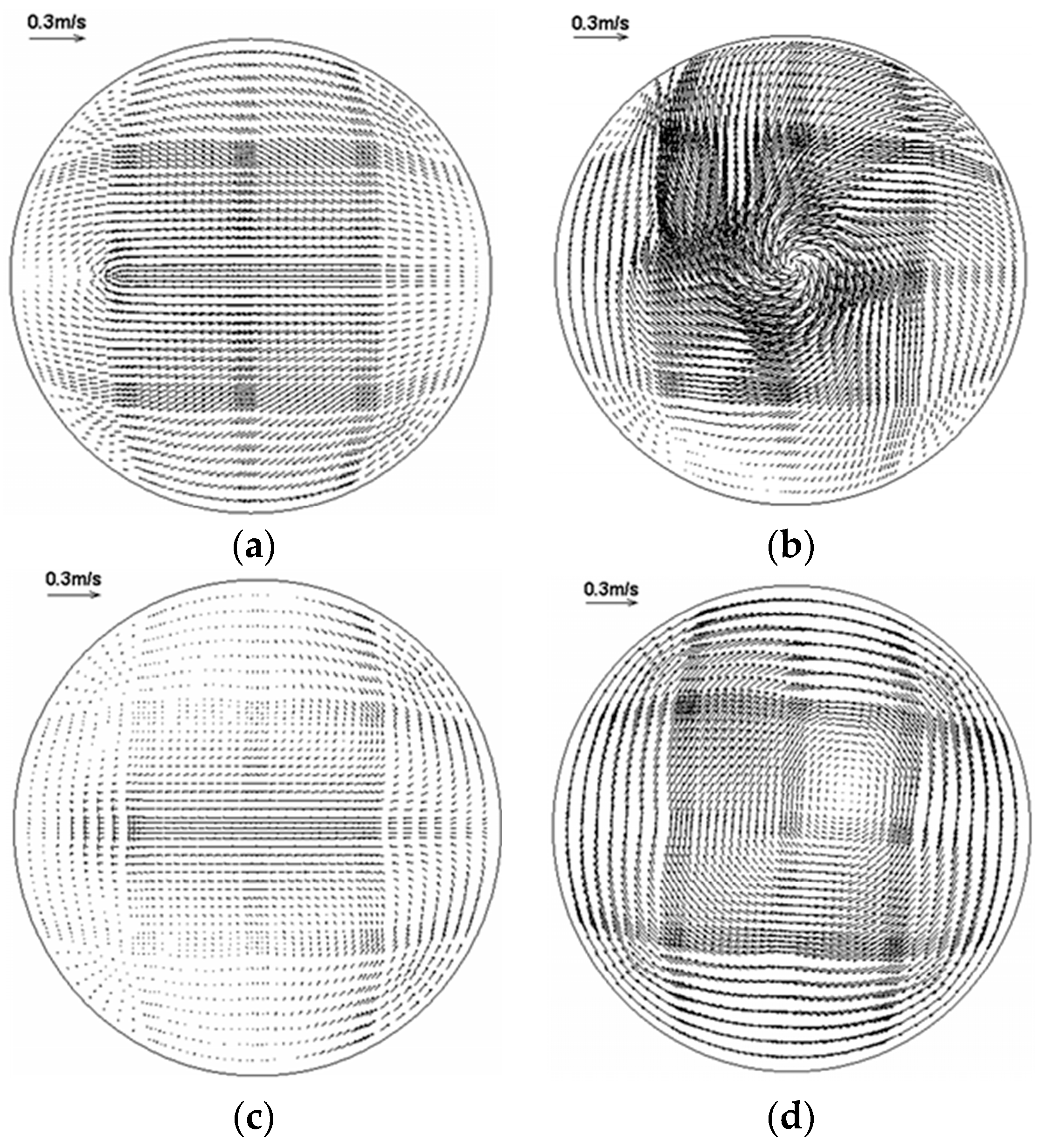
The analysis regarding the flow field is based on the results of transient simulation at 360 s. Figure 4 illustrates the velocity vector of molten steel on Z = 0.1 m and Z = 2 m sections for non-EMS and bottom-rotating EMS. The velocity magnitudes for the case without EMS on Z = 0.1 m and Z = 2 m section are smaller compared with the results obtained from the case with bottom-rotating EMS applied, which implies that dead zones easily form and result in the stratification of temperature and concentration in those regions. The phenomena have adverse effects on improving the product quality. When the bottom-rotating EMS is adopted, the rotating EMF rotates the molten steel near the bottom of the ladle, and the shear force further drives the bulk to in rotational motion, as shown in Figure 4b,d. As a result, the flow field of molten steel is improved significantly.
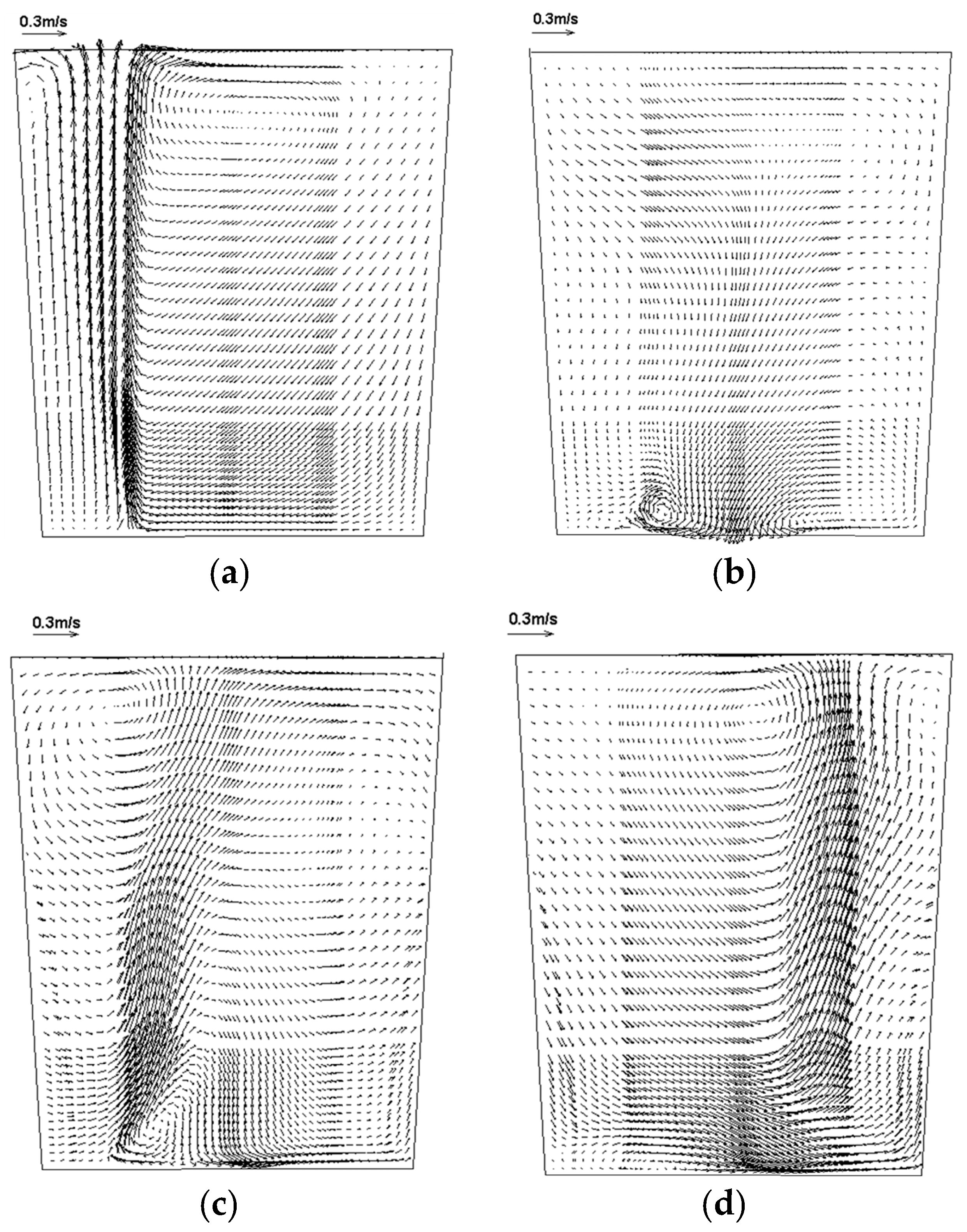
Figure 5a shows the flow pattern on Y = 0 m section without EMS. As depicted, the region with high velocity settles over the argon inlet. The fluid flows upward to the top surface and forms a circulatory flow. This could be attributed to the fact that argon gas bubbles would float upward and escape from the top surface after being jetted from the inlet. As a result, the fluid is driven to flow upward and a circulatory flow is formed due to the interaction force between bubbles and molten steel. Figure 5b–d respectively show the flow pattern with bottom-rotating EMS on Y = 0 m section, Y = 0.5 m and X = −0.4 m section. Figure 5b shows that the flow direction of molten steel is downward near the neighborhood of the agitator, this is because the centrifugal effect caused by the rotating flow of fluid forms a lower pressure region, and resultantly, the fluid in the high pressure region moves along the pressure gradient and down toward the low pressure region. After the bottom-rotating EMS has been applied, the notable upward flow disappears on the Y = 0 m section, but the upward flow is manifested on the section of Y = 0.5 m and X = −0.4 m. It follows that the flow pattern is deflected under the effect of bottom-rotating EMS. The phenomena implies the combined method is beneficial to improve the distal flow and reduce the dead zone inside the ladle.
Figure 6 shows the isosurface of VAr = 1.0 × 10⁻⁴ (volume fraction of argon) for non-EMS and bottom-rotating EMS with the current I = 600 A and I = 1200 A at 360 s. The whole shape of isosurface remains columnar when absent of EMS. It implies the impingement effect caused by the argon bubbles floating upward and passing through the slag layer is intense, which makes it easier to form open-eye and causes re-oxidation and slag entrapment near the slag layer. It is evident from Figure 6b,c, with the employment of the bottom-rotating EMS, the isosurface occurs significant deviation and the isosurface further extends and deflects when the current reaches 1200 A. The gas-liquid two phase region is extended with increasing current intensity, which is beneficial to remove inclusions and reduce the impingement of argon bubbles on the free surface.
Figure 7 shows the trajectory of argon gas bubbles at 420 s. When the bottom-rotating EMS is not applied, the bubbles float upward under the action of buoyancy after the ejection from the porous plug. Its trajectory is linear with little deflection. When the bottom-rotating EMS is applied, the molten steel near the bottom of ladle is driven by the rotating EMF and further promotes rotational motion. Due to the effect of the interaction between the gas and molten steel, the trajectory of bubbles gets deflected along with the tangent direction of the flow and, as a result, the distribution of bubbles become more dispersed. This phenomenon is useful in prolonging the residence time of argon gas bubbles and reducing the impact of bubbles on the slag layer. The water model experiment verifies the identical phenomenon according to Figure 8.
Figure 9 illustrates the distribution of the molten steel turbulence kinetic energy (TKE) on the Z = 3.7 m section near the top surface. A significant gradient of TKE is observed without EMS, which indicates that the intense impact caused by argon bubbles floating upward and passing through the slag layer appears near the free surface. When the bottom-rotating EMS is adopted, the high-TKE region is prone to deflection. The high-TKE region tends to reduce with the increasing current intensity, and in particular, the region enduring a TKE of 0.1 disappears as the current intensity reaches 1200 A. It may be interpreted that the rotating flow disperses argon bubbles and reduces the impingement of argon bubbles on the slag layer, which is beneficial to decrease the open-eye and slag entrapment.
4.3. Analysis of Temperature Field
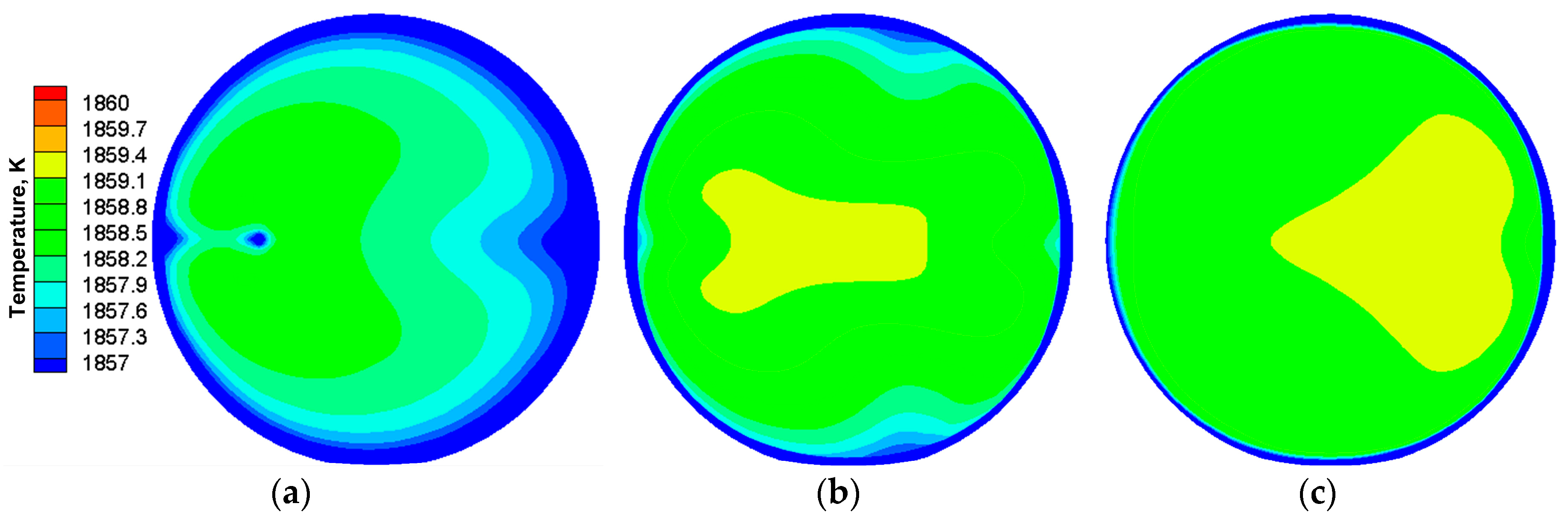
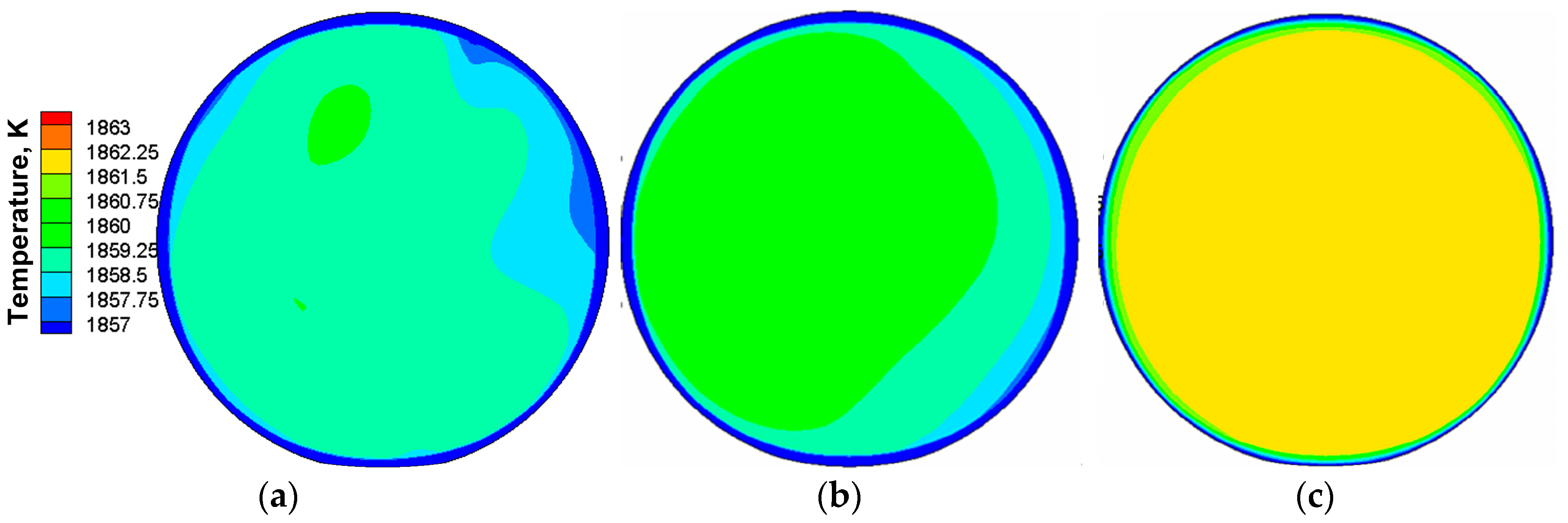
The analysis of temperature field is based on the results of transient simulation at 360 s. The distribution of temperature for non-EMS and bottom-rotating EMS on Z = 0.3 m, Z = 2.0 m, and Z = 3.7 m sections are shown in Figure 10 and Figure 11, respectively. As shown in Figure 10a,b, a wide region with a lower temperature close to the ladle wall and the porous plug is found. The case without EMS indicates a distinct temperature stratification. The two reasons for this phenomenon, one is the heat transfer around ladle wall and the heat absorption of lower temperature argon gas, and another is that the stirring intensity of argon into molten steel is insufficient. After applying the bottom-rotating EMS, the lower temperature region is decreased and the temperature stratification is clearly improved as shown from Figure 11a,b. This is mainly because the thermal effect of the alternating magnetic field partly compensates the heat loss of molten steel and the combination of AGS and the bottom-rotating EMS improves the flow field of molten steel. With the flow field fully mixed, the top surface approaches a uniform temperature distribution according to Figure 10c and Figure 11c. Due to the thermal compensation, the temperature for using the bottom-rotating EMS is slightly higher than that for non-EMS.
Figure 12 shows the distribution of temperature near the middle of the ladle (Z = 2 m section) with a different current intensity. It is clear that there is a clear temperature gradient with higher temperature in the center of ladle and lower temperature near the ladle wall when the current intensity is 300 A. However, in Figure 12a–c, the highest temperature region expands with the current intensity due to the heating effect and improved flow. The distribution of temperature tends to be uniform and the value of the temperature reaches 1862.25 K as the current intensity reaches 1200 A. Therefore, increasing the current intensity is beneficial for compensating the heat loss and eliminating the temperature stratification of molten steel in a ladle.
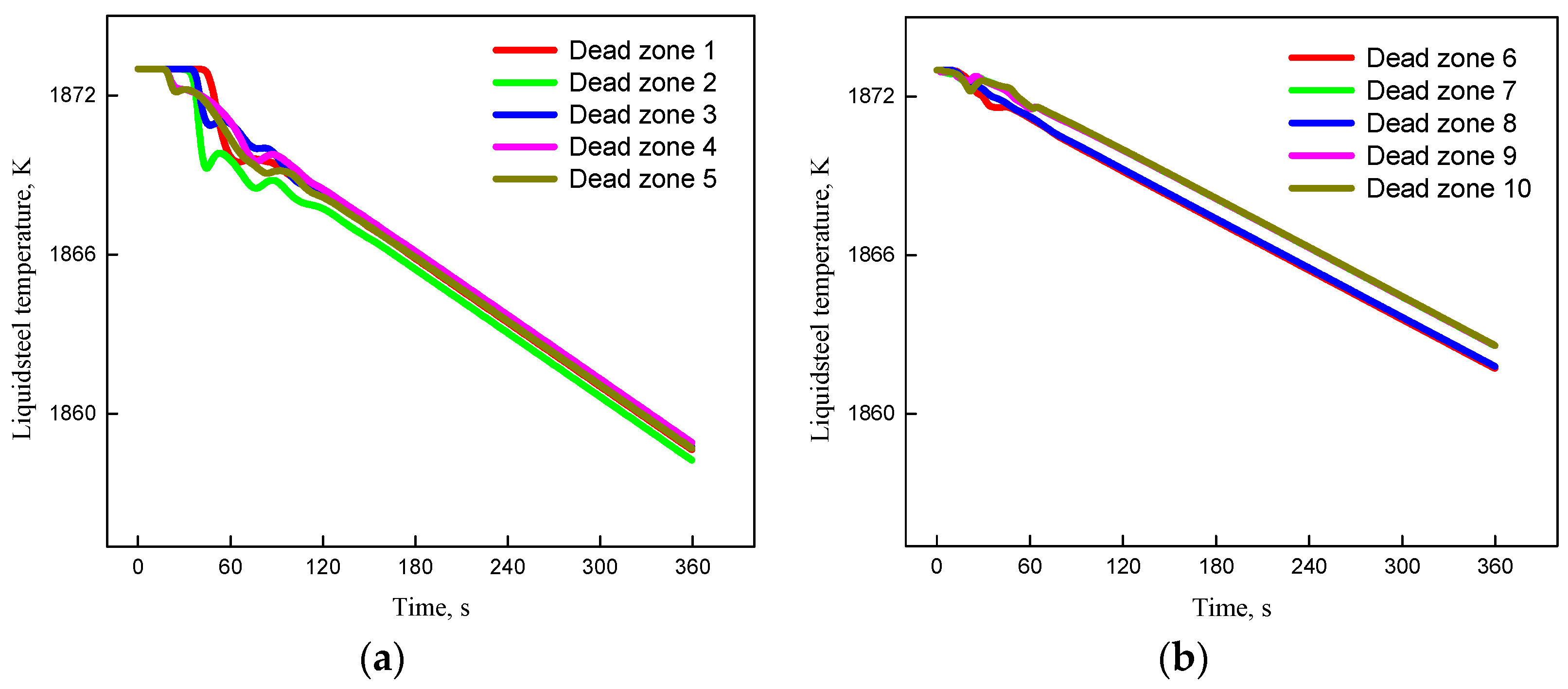
In order to investigate the temperature change in the dead zone, points within different dead zones were monitored and their temperature change with time was analyzed. The distribution and location of the points are shown in Figure 13 and Table 3. The results are shown in Figure 14a,b, where Figure 14a shows the case of non-EMS and Figure 14b shows the case of a combined method with current of 1200 A. As shown in Figure 14a, the temperature at each point of the dead zones decreases steadily and the average temperature drops from 1873 K to 1858.7 K in six minutes. The average temperature drop is about 2.38 K/min. After applying bottom-rotating EMS, the average temperature of each point declines from 1873 K to 1862.9 K and the average temperature drop is about 1.68 K/min according to Figure 14b. Therefore, the increasing current intensity is favorable for keeping the temperature of molten steel steady.
4.4. Analysis of Concentration Field
To research the influence of the combined method on the alloy concentration distribution behavior, manganese alloy was selected as a tracer material and added at a speed of 59.65 kg/s, lasting for 37 s. The normalization concentration was used and can be expressed as CNom = (C − C0)/(C∞ − C0), where C is the alloy concentration at a particular time, C0 is the initial alloy concentration with its value of 0 kg·m−3 and C∞ is the alloy equilibrium concentration [29] in the molten steel. Figure 15 illustrates the normalization concentration contour after the adding alloy at t = 40 s and t = 100 s.
As shown in Figure 15a at t = 40 s, the alloy assembles at the top surface of ladle due to its relatively small density when compared with molten steel. Under the action of molten steel circulatory flow, as shown in Figure 5a, the alloy is involved in the whole circulatory flow and diffuses gradually to the interior of the molten steel. Due to the intense circulatory flow on the vertical section, the alloy is well mixed in this region and, according to Figure 15a at t = 100 s, its normalization concentration almost reaches 1. There is concentration stratification on both sides of the main circulatory flow and nearby the wall due to the weakened flow.
The case of bottom-rotating EMS with the alloy depositing site situating point (−1.3, 0, 3.732), at t = 40 s and t = 100 s have serious concentration stratification according to Figure 15b. The alloy is mainly concentrated in the upper half of the ladle, which implies the alloy cannot participate in the main circulatory flow of molten steel. The reason is that the gas-liquid plume is deflected due to the rotating EMF, which results in an untraceable alloy depositing site in the molten steel circulatory flow. Figure 15c shows the case of the alloy depositing site situating point (0.38, 0.58, 3.732), the concentration is more uniform than that of others at t = 40 s. Since the alloy depositing site is located in the area of the argon gas escape, the alloy is involved in the circulatory flow and rapidly diffuses into the molten steel. When the mixing time reaches 100 s, the alloy in the middle and upper part of the ladle is fully mixed, but there is a slight concentration stratification near the bottom of the ladle. As a whole, its mixture effect of the combined method is superior to the single argon gas stirring method due to the improved flow field and fewer dead zones in the ladle. However, the site of depositing alloy needs to be adjusted according to the whole circulatory flow and the position of argon to escape.
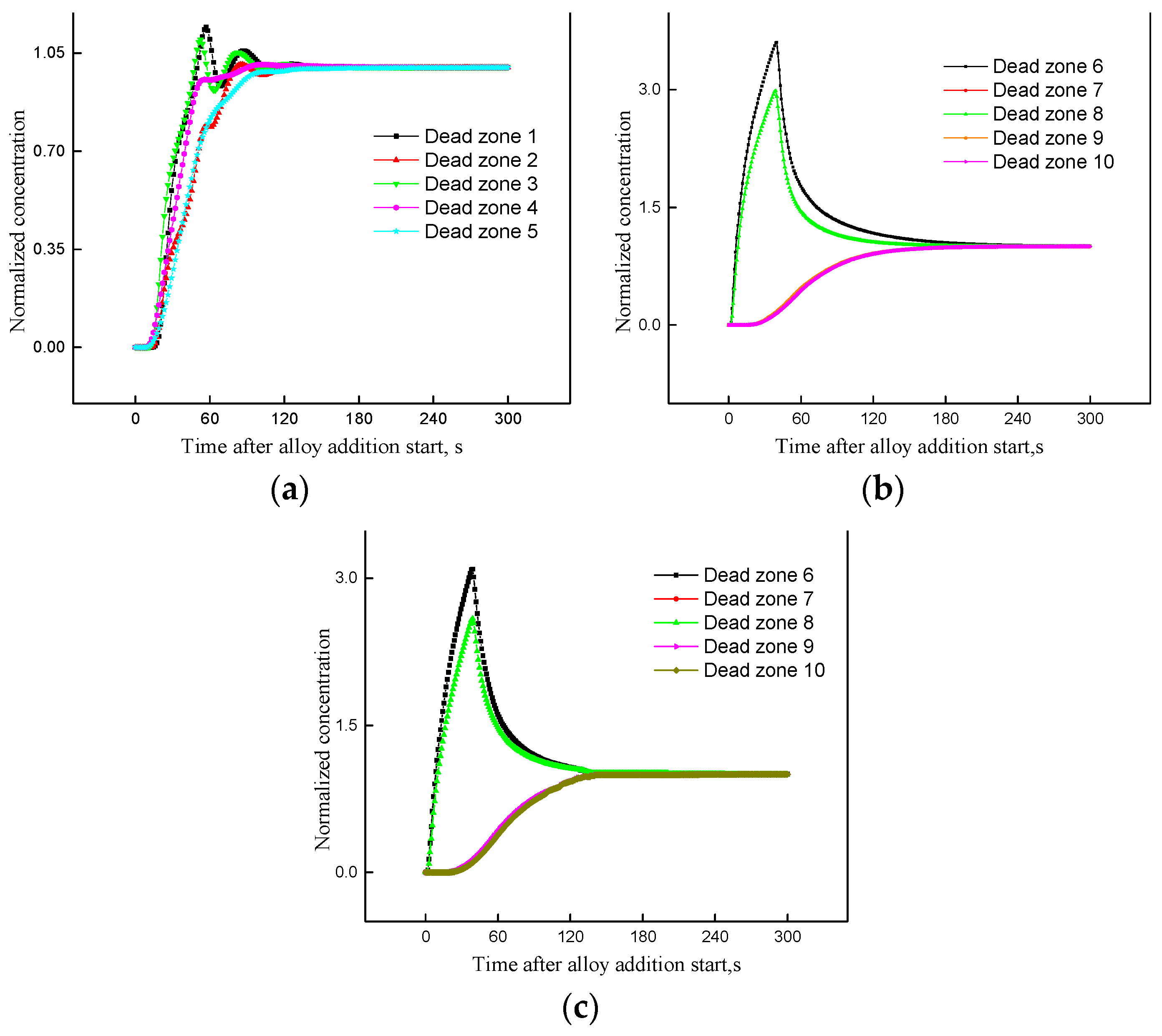
Figure 16a–c illustrates the distribution of normalization concentration along time at different dead zone points. Figure 16a is the case of the single argon gas stirring with the alloy depositing site situating point (−1.3, 0, 3.732). It is shown that the change of each point is the same. When the alloy is added, the normalization concentration increases linearly in the former 50 s, and reaches 1 at 160 s, which indicates the alloy becomes fully mixed in the ladle. Figure 16b,c are the cases with the combined method. For the former, the alloy depositing site is at point (−1.3, 0, 3.732), and for the latter, the depositing site is at the point (−0.38, 0.58, 3.732). The curves of test points 6 and 8 show a tendency to increase and then decrease due to the location of the test point in the upper part of ladle. The curves of test point 7, 9, and 10 are almost coincident, which implies there is the same flow on this test point. The time of full mixture is about 230 s for case 2 and 140 s for case 3 as shown from Figure 16b,c. The full mixing time is shortened from 230 s to 140 s when the depositing alloy site situates the point (−0.38, 0.58, 3.732). Comparing case 1 and case 3, the mixing time of combined method is less than that with the single argon gas stirring method. Therefore, the combined method is beneficial to accelerate the dispersion of additive agent and improve the quality of products in the industry process.
5. Conclusions
Numerical simulation and a water model experiment were carried out to investigate the influence of the combined argon gas stirring method and bottom-rotating EMS on fluid flow, the distribution of temperature, and the concentration in a ladle, respectively. The conclusions can be summarized as follows:
- (1)
- The electromagnetic force consists of a horizontal component spinning clockwise and vertical component upwards. Current intensity plays a critical role on the magnitude of electromagnetic force.
- (2)
- After the combined method is imposed, the gas-liquid plume region is deflected and expanded, and the EMF-driven rotational flow has positive influence of improving the dispersion of bubbles, which contribute to prolonging the residence time of bubbles and weaken the impingement effect of bubbles on the slag layer.
- (3)
- When the combined method is adopted, the temperature stratification tends to alleviate due to the effect of heat compensation and the improved flow. The temperature stratification tends to disappear when the current reaches 1200 A.
- (4)
- The improved flow has a positive influence on decreasing concentration stratification and shortening the mixing time when the combined method is used. However, the alloy depositing site needs to be optimized according to the whole circulatory flow and the region of bubbles to escape.
Acknowledgments
This work was supported by National Natural Science Foundation of China (No. 51474065, 51574083), the Doctoral Scientific Research Foundation of Liaoning Province of China (No. 20141008), and the Program of Introducing Talents of Discipline to Universities of China (No. B07015).
Author Contributions
Anyuan Deng conceived and designed the study. Yang Li and Huan Li performed the simulations and contributed to the result analysis. Engang Wang and Bin Yang contributed to the experiment data. Yang Li wrote the manuscript.
Conflicts of Interest
The authors declare no conflict of interest.
Nomenclature
| A | Magnetic vector potential (Wb·m) | Re | Real part of a complex quantity |
| B | Magnetic flux density (T) | Reb | Bubble Reynolds number (dimensionless) |
| C | Mass fraction of the species (dimensionless) | Rem | Magnetic Reynolds number (dimensionless) |
| CD | Drag force coefficient (dimensionless) | SCt | Turbulent Schmidt number (dimensionless) |
| CL | Lift force coefficient (dimensionless) | t | Time (s) |
| cp | Specific heat capacity at constant pressure (J·kg−1·K−1)) | T | Temperature (K) |
| CTD | Turbulent dispersion coefficient (dimensionless) | ub | Velocity of argon bubble (m·s−1) |
| CVM | Virtual mass force coefficient (dimensionless) | ug | Velocity of the gas phase (m·s−1) |
| Cμ,T | Model constant (dimensionless) | ul | Velocity of the liquid phase (m·s−1) |
| Cε1 | Model constant (dimensionless) | xb | Displacement of argon bubble (m) |
| Cε2 | Model constant (dimensionless) | ||
| D0 | Diffusion coefficient (m2·s−1) | Greek symbols | |
| db | Diameter of argon bubble (m) | α | Volume fraction (dimensionless) |
| E | Electric field intensity (V·m−1) | ε | Turbulent dissipation rate (m2·s−3) |
| FB | Buoyancy force (N·m−3) | λ | Thermal conductivity (W·m−1·K−1) |
| FD | Drag force (N·m−3) | η | Magnetic permeability (H·m−1) |
| FEM | Electromagnetic repulsive force (N·m−3) | μeff | Effective viscosity of the fluid (kg·m−1·s−1) |
| FL | Lift force (N·m−3) | μT,l | Turbulent eddy viscosity (kg·m−1·s−1) |
| Fmag | Lorentz force (N·m−3) | μl | Dynamic viscosity of liquid phase (kg·m−1·s−1) |
| FP | Pressure gradient force (N·m−3) | ρg | Density of the argon gas (kg·m−3) |
| FTD | Turbulent dispersion force (N·m−3) | ρl | Density of the molten steel (kg·m−3) |
| FVM | Virtual mass force (N·m−3) | σ | Electrical conductivity (S·m−1) |
| FWL | Wall lubrication force (N·m−3) | σk | Model constant (dimensionless) |
| g | Gravitational acceleration (m·s−2) | σε | Model constant (dimensionless) |
| H | Magnetic intensity (A·m−1) | σT,l | Turbulent Schmidt number (dimensionless) |
| J | Current density (A·m−2) | φ | Electric scalar potential (V) |
| Je | Induced current density (A·m−2) | ω | Angular frequency (rad·s−1) |
| Js | Source current density (A·m−2) | Subscript | |
| k | Turbulent kinetic energy (m2·s−2) | l | Liquid phase |
| p | Pressure (Pa) | g | Gas phase |
| Qv | Joule heat (W·m−3) | b | Argon gas bubble |
References
- Wu, L.; Valentin, P.; Sichen, D. Study of Open Eye Formation in an Argon Stirred Ladle. Steel Res. Int. 2010, 81, 508–515. [Google Scholar] [CrossRef]
- Alexis, J.; Jonsson, P.; Jonsson, L. Heating and electromagnetic stirring in a ladle furnace—A simulation model. ISIJ Int. 2000, 40, 1098–1104. [Google Scholar] [CrossRef]
- Dayal, P.; Beskow, K.; Bjorkvall, J.; Sichen, D. Study of stag/metal interface in ladle treatment. Ironmak. Steelmak. 2006, 33, 454–464. [Google Scholar] [CrossRef]
- Huang, A.; Harmuth, H.; Doletschek, M.; Vollmann, S.; Feng, X. Toward CFD Modeling of Slag Entrainment in Gas Stirred Ladles. Steel Res. Int. 2015, 86, 1447–1454. [Google Scholar] [CrossRef]
- Inomoto, T.; Ogawa, Y.; Toh, T. Promotion of desulphurization in ladle through slag emulsification by stirring with stationary AC electromagnetic field. ISIJ Int. 2003, 43, 828–835. [Google Scholar] [CrossRef]
- Xu, Y.; Ersson, M.; Jonsson, P.G. A Mathematical Modeling Study of Bubble Formations in a Molten Steel Bath. Metall. Mater. Trans. B 2015, 46, 2628–2638. [Google Scholar] [CrossRef]
- Delobelle, P.; Oytana, C. Study of slag/metal interface in ladle treatment. Ironmak. Steelmak. 2013, 33, 454–464. [Google Scholar]
- Li, B.; Yin, H.; Zhou, C.Q.; Tsukihashi, F. Modeling of Three-phase Flows and Behavior of Slag/Steel Interface in an Argon Gas Stirred Ladle. Trans. Iron Steel Inst. Jpn. 2008, 48, 1704–1711. [Google Scholar] [CrossRef]
- Thunman, M.; Eckert, S.; Hennig, O.; Björkvall, J.; Du, S. Study on the Formation of Open-Eye and Slag Entrainment in Gas Stirred Ladle. Steel Res. Int. 2007, 78, 849–856. [Google Scholar] [CrossRef]
- Ramírez-Argáez, M.A. Numerical Simulation of Fluid Flow and Mixing in Gas-Stirred Ladles. Mater. Manuf. Process. 2007, 23, 59–68. [Google Scholar] [CrossRef]
- Warzecha, W.; Jowsa, J.; Merder, T. Gas Mixing And Chemical Homogenization of Steel In 100 T Ladle Furnace. Metalurgija 2007, 46, 227–232. [Google Scholar]
- Llanos, C.A.; Saul, G.H.; Angel, R.B.J.; Barreto, J.D.J.; Gildardo, S.D. Multiphase Modeling of the Fluidynamics of Bottom Argon Bubbling during Ladle Operations. ISIJ Int. 2010, 50, 396–402. [Google Scholar] [CrossRef]
- Geng, D.Q.; Lei, H.; He, J.C. Numerical Simulation for Collision and Growth of Inclusions in Ladles Stirred with Different Porous Plug Configurations. ISIJ Int. 2010, 50, 1597–1605. [Google Scholar] [CrossRef]
- Joo, S.; Guthrie, R.I.L. Modeling flows and mixing in steelmaking ladles designed for single- and dual-plug bubbling operations. Metall. Trans. B 1992, 23, 765–778. [Google Scholar] [CrossRef]
- Mietz, J.; Oeters, F. Model experiments on mixing phenomena in gas-stirred melts. Steel Res. 1988, 59, 52–59. [Google Scholar] [CrossRef]
- Tang, H.; Guo, X.; Wu, G.; Wang, Y. Effect of Gas Blown Modes on Mixing Phenomena in a Bottom Stirring Ladle with Dual Plugs. ISIJ Int. 2016, 12, 2161–2170. [Google Scholar]
- Chung, S.I.; Shin, Y.H.; Yoon, J.K. Flow Characteristics by Induction and Gas Stirring in ASEA-SKF Ladle. ISIJ Int. 1992, 32, 1287–1296. [Google Scholar] [CrossRef]
- Sand, U.; Yang, H.L.; Eriksson, J.E.; Fdhila, R.B. Numerical and Experimental Study on Fluid Dynamic Features of Combined Gas and Electromagnetic Stirring in Ladle Furnace. Steel Res. Int. 2009, 80, 441–449. [Google Scholar]
- Liu, H.; Qi, Z.; Xu, M. Numerical Simulation of Fluid Flow and Interfacial Behavior in Three-phase Argon-Stirred Ladles with One Plug and Dual Plugs. Steel Res. Int. 2011, 82, 440–458. [Google Scholar] [CrossRef]
- Wang, Q.; Yao, W. Computation and validation of the interphase force models for bubbly flow. Int. J. Heat Mass Transf. 2016, 98, 799–813. [Google Scholar] [CrossRef]
- Drew, D.A.; Lahey, R.T. The virtual mass and lift force on a sphere in rotating and straining inviscid flow. Int. J. Multiph. Flow 1987, 13, 113–121. [Google Scholar] [CrossRef]
- Burns, A.D.; Frank, T.; Hamill, I.; Shi, J.M. The Favre averaged drag model for turbulent dispersion in Eulerian multi-phase flows. In Proceedings of the Fifth International Conference on Multiphase Flow, Yokohama, Japan, 30 May–4 June 2004; pp. 391–392. [Google Scholar]
- Launder, B.E.; Spalding, D.B. The numerical computation of turbulent flows. Comput. Methods Appl. Mech. Eng. 1974, 3, 269–289. [Google Scholar] [CrossRef]
- Lou, W.; Zhu, M. Numerical Simulation of Gas and Liquid Two-Phase Flow in Gas-Stirred Systems Based on Euler–Euler Approach. Metall. Mater. Trans. B 2013, 44, 1251–1263. [Google Scholar] [CrossRef]
- Moreau, R. Magnetohydrodynamics; Kluwer Academic Pbulishers: Dordrecht, The Netherlands, 1990; p. 37. [Google Scholar]
- Jiang, D.; Zhu, M. Flow and Solidification in Billet Continuous Casting Machine with Dual Electromagnetic Stirrings of Mold and the Final Solidification. Steel Res. Int. 2015, 86, 993–1003. [Google Scholar] [CrossRef]
- Sivak, B.A.; Grachev, V.G.; Parshin, V.M.; Chertov, A.D.; Zarubin, S.V.; Fisenko, V.G.; Solov’Ev, A.A. Magnetohydrodynamic processes in the electromagnetic mixing of liquid phase in the ingot on continuous bar- and bloom-casting machines. Steel Transl. 2009, 39, 774–782. [Google Scholar] [CrossRef]
- Leenov, D.; Kolin, A. Theory of Electromagnetophoresis. I. Magnetohydrodynamic Forces Experienced by Spherical and Symmetrically Oriented Cylindrical Particles. J. Chem. Phys. 1954, 22, 683–688. [Google Scholar] [CrossRef]
- Ni, S.; Wang, H.; Zhang, J.; Lin, L.; Chu, S. A Novel Criterion of Mixing Time in Gas-Stirred Ladle Systems. Acta Metall. Sin. 2014, 27, 1008–1011. [Google Scholar] [CrossRef]
Figure 1.
Geometric model of the ladle-combined AGS and bottom-EMS.
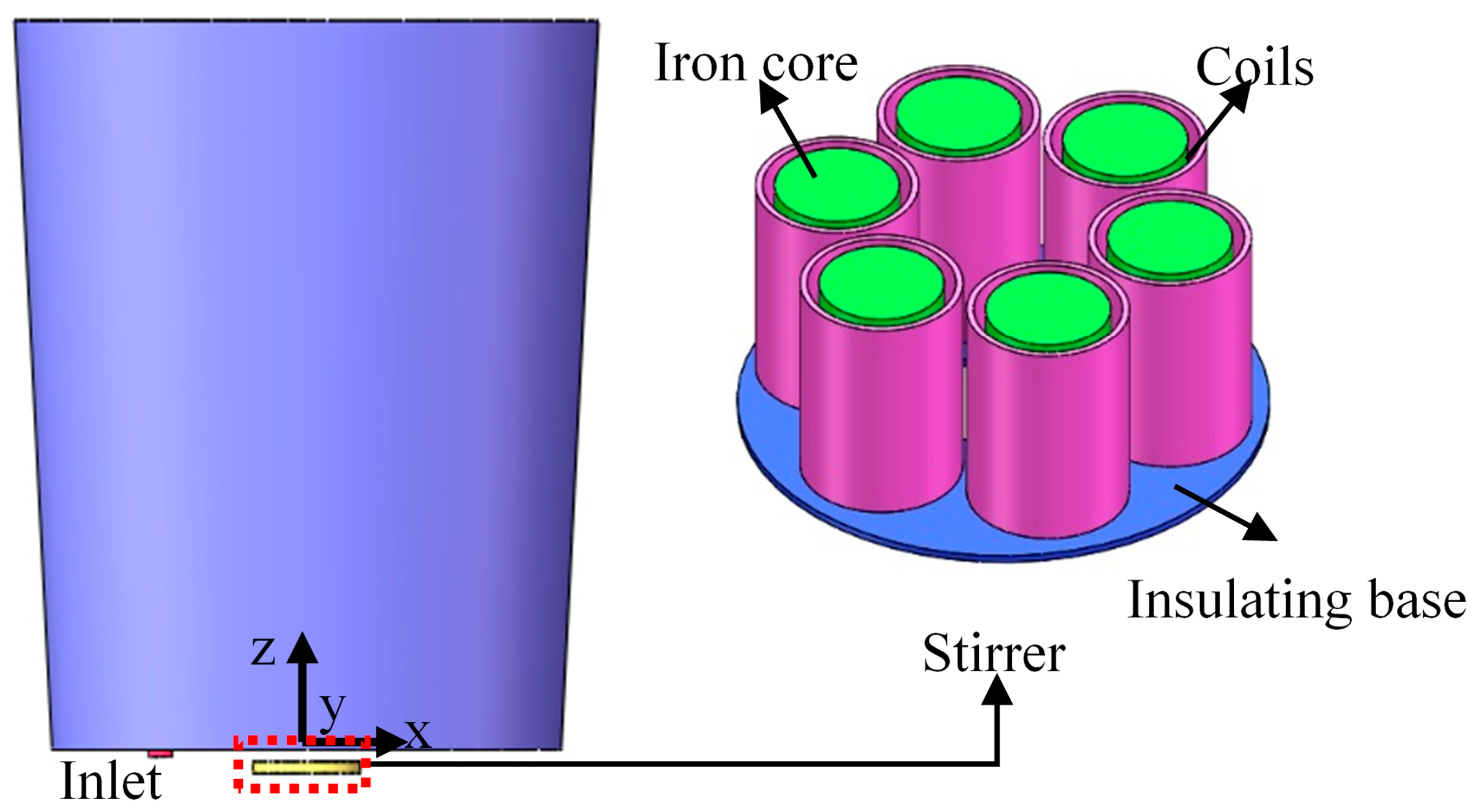
Figure 2.
Distribution of electromagnetic force (EMF) on (a) the bottom surface (Z = 0 m) and (b) the central section (Y = 0 m).
Figure 2.
Distribution of electromagnetic force (EMF) on (a) the bottom surface (Z = 0 m) and (b) the central section (Y = 0 m).
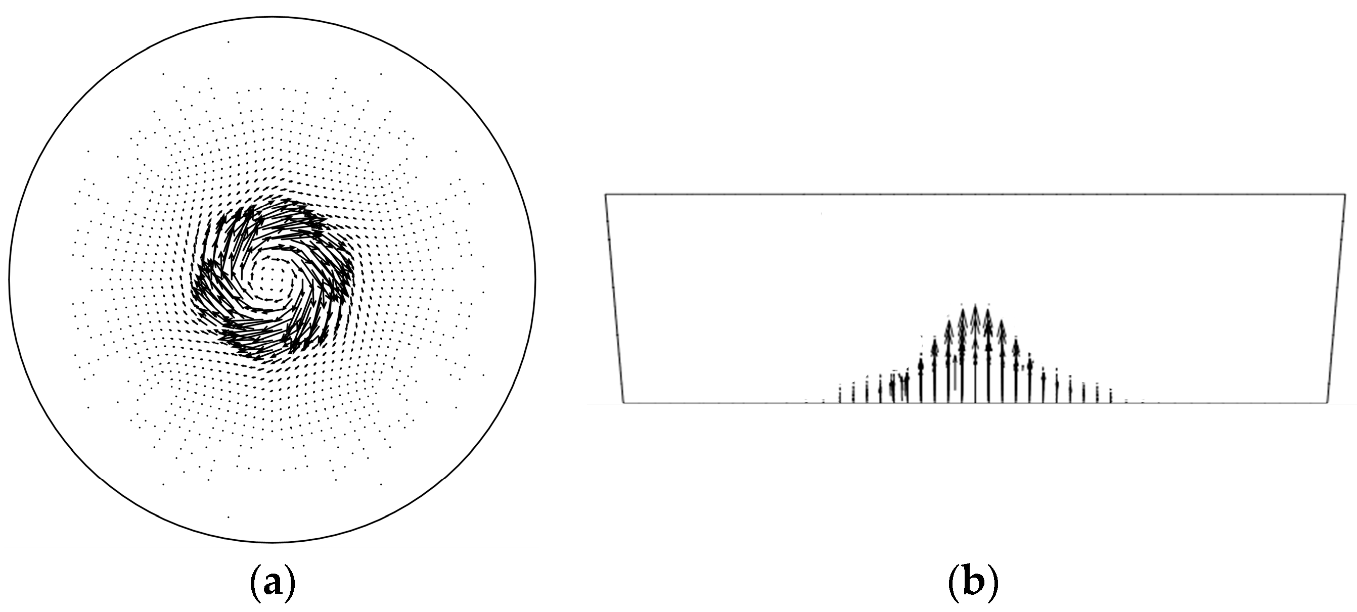
Figure 3.
Distribution of the EMF magnitude for different current intensities with a fixed frequency of 50 Hz (a), and different frequencies with a fixed current intensity of 1200 A (b) along the radial direction.
Figure 3.
Distribution of the EMF magnitude for different current intensities with a fixed frequency of 50 Hz (a), and different frequencies with a fixed current intensity of 1200 A (b) along the radial direction.

Figure 4.
Distribution of the flow field at 360 s ((a,b) are non-EMS and bottom-rotating EMS at I = 300 A on Z = 0.1 m section, respectively; (c,d) are non-EMS and bottom-rotating EMS at I = 300 A on Z = 2 m section, respectively).
Figure 4.
Distribution of the flow field at 360 s ((a,b) are non-EMS and bottom-rotating EMS at I = 300 A on Z = 0.1 m section, respectively; (c,d) are non-EMS and bottom-rotating EMS at I = 300 A on Z = 2 m section, respectively).

Figure 5.
Distribution of the flow field at 360 s ((a) is Y = 0 m section for non-EMS, (b–d) is, respectively, Y = 0 m, Y = 0.5 m and X = 22,120.4 m section for bottom-rotating EMS at I = 300 A).
Figure 5.
Distribution of the flow field at 360 s ((a) is Y = 0 m section for non-EMS, (b–d) is, respectively, Y = 0 m, Y = 0.5 m and X = 22,120.4 m section for bottom-rotating EMS at I = 300 A).

Figure 6.
Isosurface of the argon volume fraction VAr = 1.0 × 10⁻⁴ at 360 s ((a) for non-EMS, (b,c) for bottom-rotating EMS at I = 600 A and I = 1200 A).
Figure 6.
Isosurface of the argon volume fraction VAr = 1.0 × 10⁻⁴ at 360 s ((a) for non-EMS, (b,c) for bottom-rotating EMS at I = 600 A and I = 1200 A).
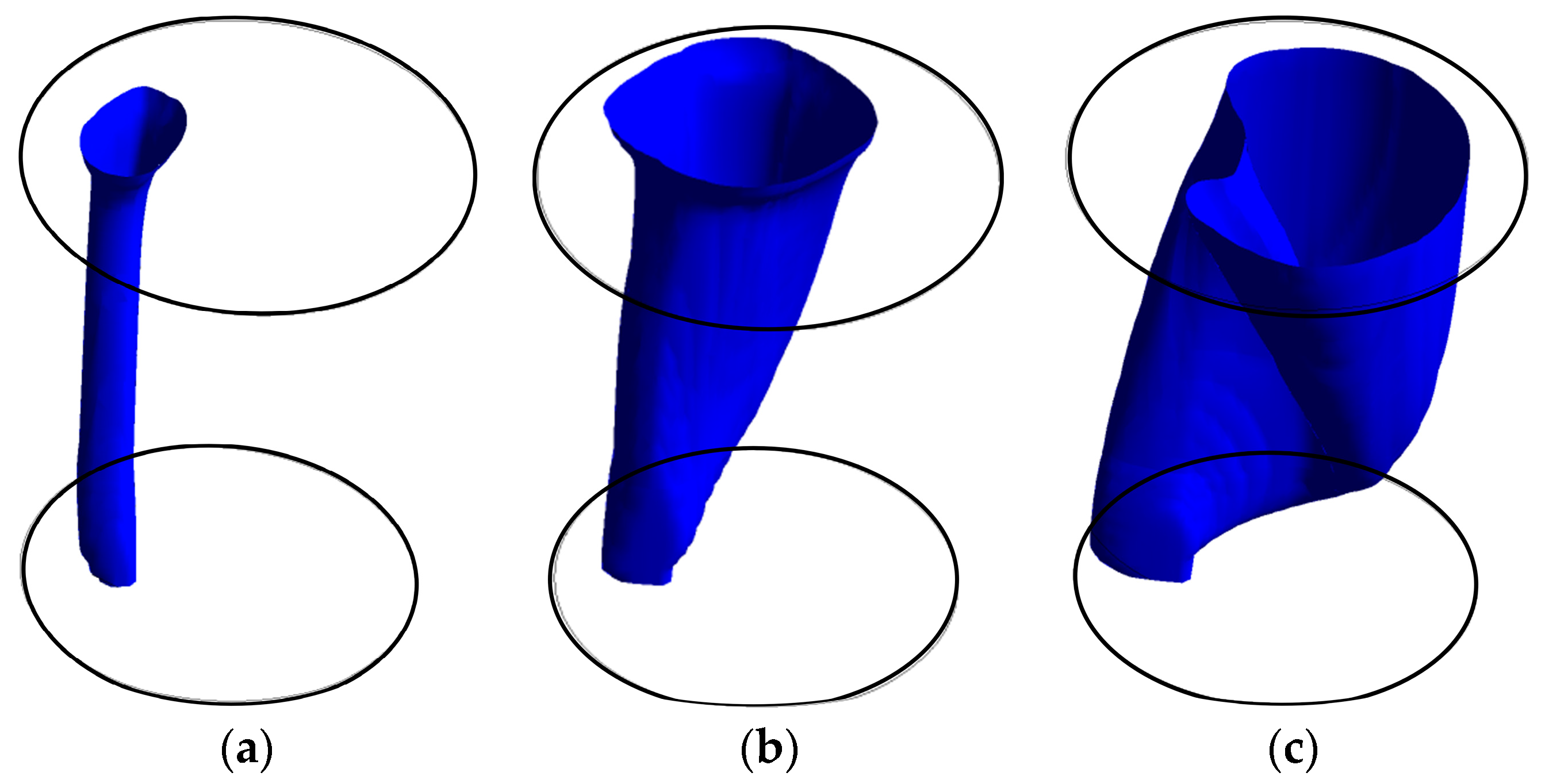
Figure 7.
Bubble trajectory at 420 s for (a) non-EMS and (b) bottom-rotating EMS at I = 600 A.

Figure 8.
Bubble trajectory on the water model experiment ((a) without stirring and (b) with bottom-rotating stirring).
Figure 8.
Bubble trajectory on the water model experiment ((a) without stirring and (b) with bottom-rotating stirring).
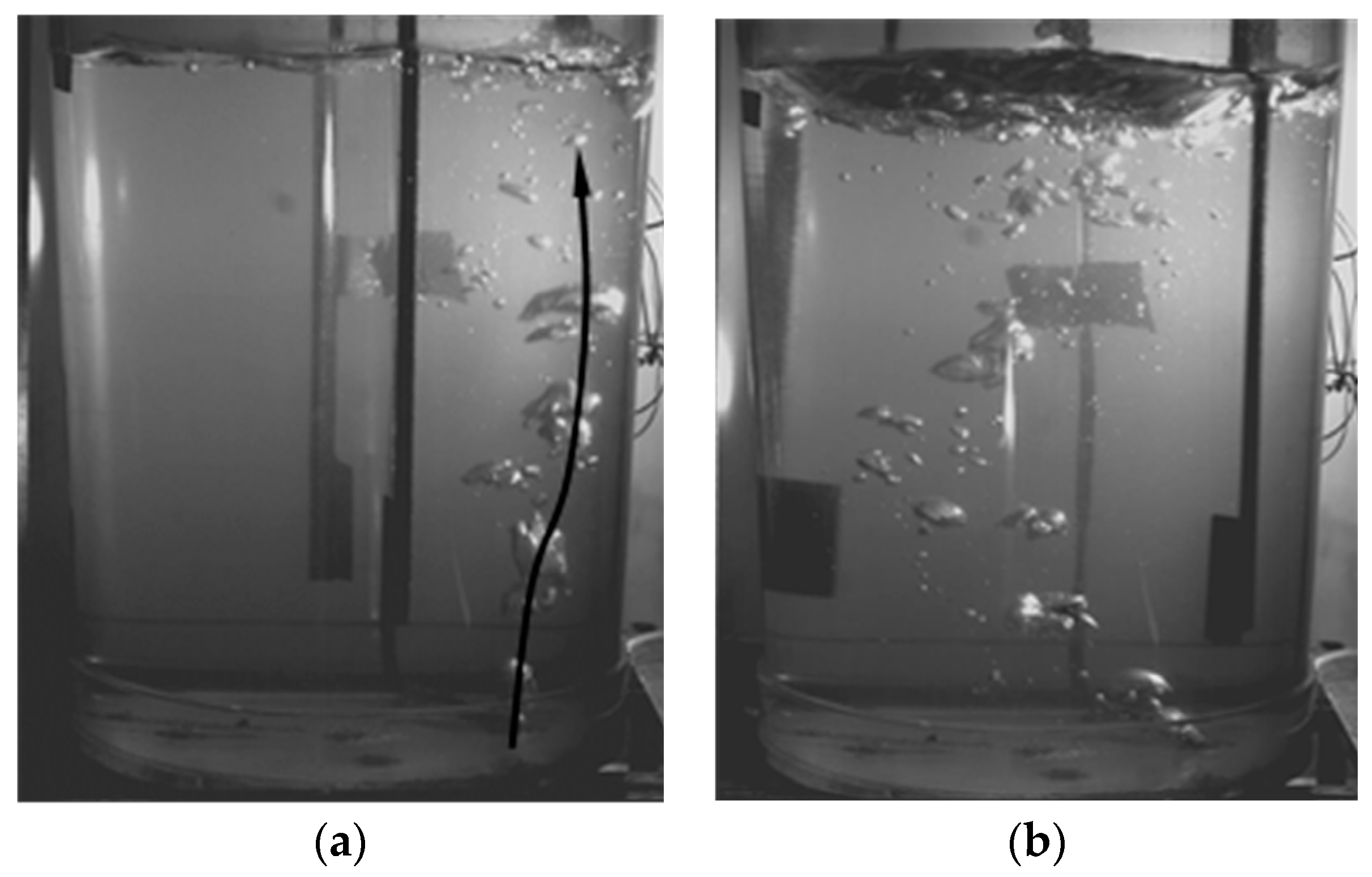
Figure 9.
Distribution of the turbulence kinetic energy on Z = 3.7 m at 360 s ((a) without stirring, (b) bottom-rotating EMS at I = 600 A, and (c) bottom-rotating EMS at I = 1200 A).
Figure 9.
Distribution of the turbulence kinetic energy on Z = 3.7 m at 360 s ((a) without stirring, (b) bottom-rotating EMS at I = 600 A, and (c) bottom-rotating EMS at I = 1200 A).
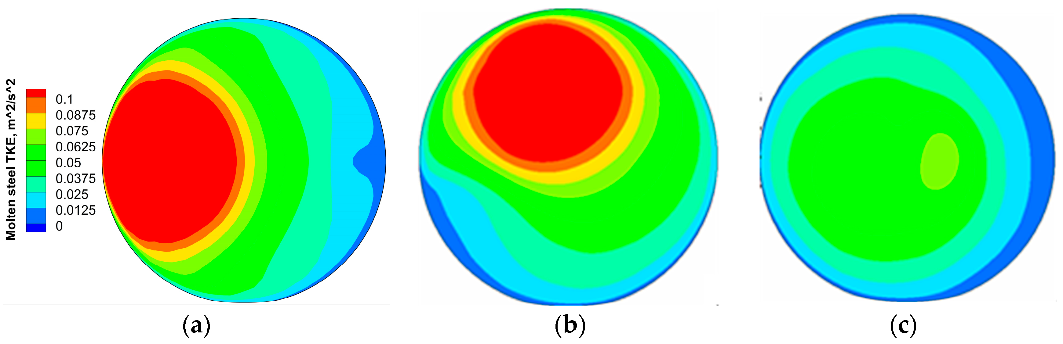
Figure 10.
Distribution of the temperature field without EMS at 360 s ((a) on Z = 0.3 m section, (b) on Z = 2 m section, and (c) on Z = 3.7 m section).
Figure 10.
Distribution of the temperature field without EMS at 360 s ((a) on Z = 0.3 m section, (b) on Z = 2 m section, and (c) on Z = 3.7 m section).

Figure 11.
Distribution of the temperature field with bottom-rotating EMS at I = 600 A at 360 s ((a) on Z = 0.3 m section, (b) on Z = 2 m section, and (c) on Z = 3.7 m section).
Figure 11.
Distribution of the temperature field with bottom-rotating EMS at I = 600 A at 360 s ((a) on Z = 0.3 m section, (b) on Z = 2 m section, and (c) on Z = 3.7 m section).
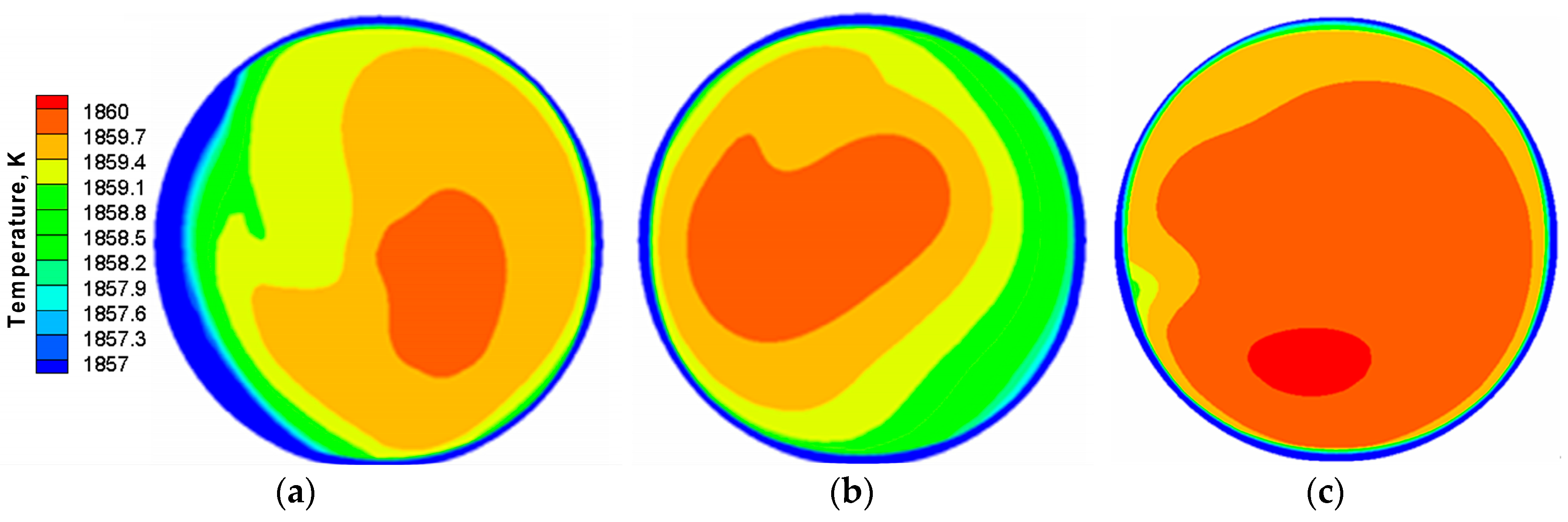
Figure 12.
Distribution of the temperature field on Z = 2 m section with bottom-rotating EMS at 360 s. (a) for 300 A, (b) for 600 A, and (c) for 1200 A.
Figure 12.
Distribution of the temperature field on Z = 2 m section with bottom-rotating EMS at 360 s. (a) for 300 A, (b) for 600 A, and (c) for 1200 A.

Figure 13.
The distribution of test point ((a) is non-EMS, and (b) is bottom-rotating EMS at 1200 A).
Figure 13.
The distribution of test point ((a) is non-EMS, and (b) is bottom-rotating EMS at 1200 A).
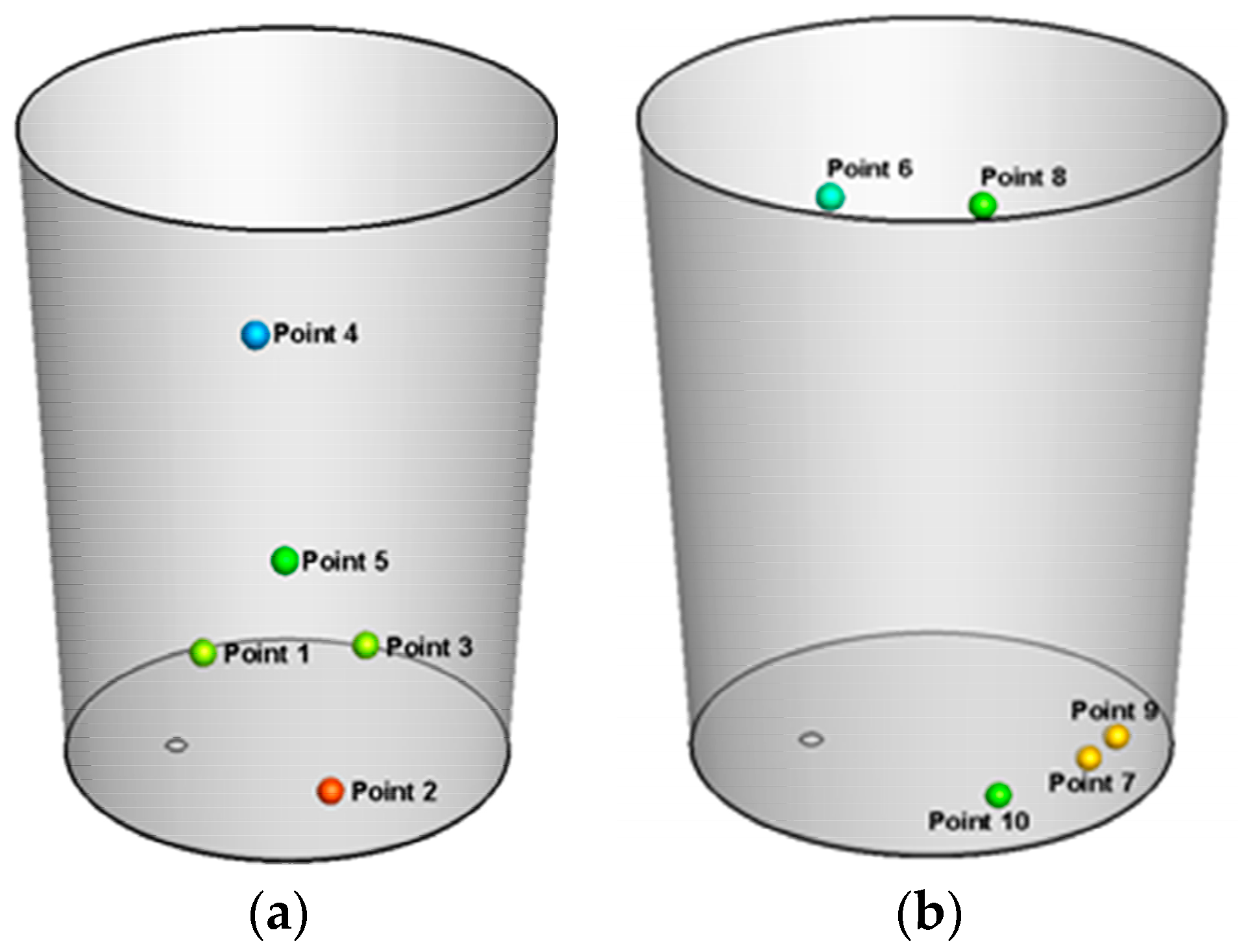
Figure 14.
Dead zone temperature changes of non-EMS (a) and the bottom-rotating EMS at 1200 A (b).

Figure 15.
Contours of the alloy normalized concentration at 40 s and 100 s ((a–c) are the non-EMS with alloy depositing site situating point (−1.3, 0, 3.732), bottom-rotating EMS at I = 600 A with alloy depositing site situating point (−1.3, 0, 3.732), and bottom-rotating EMS at I = 600 A with alloy depositing site situating point (−0.38, 0.58, 3.732) at t = 40 s, respectively; (d–f) are the same cases at t = 100 s).
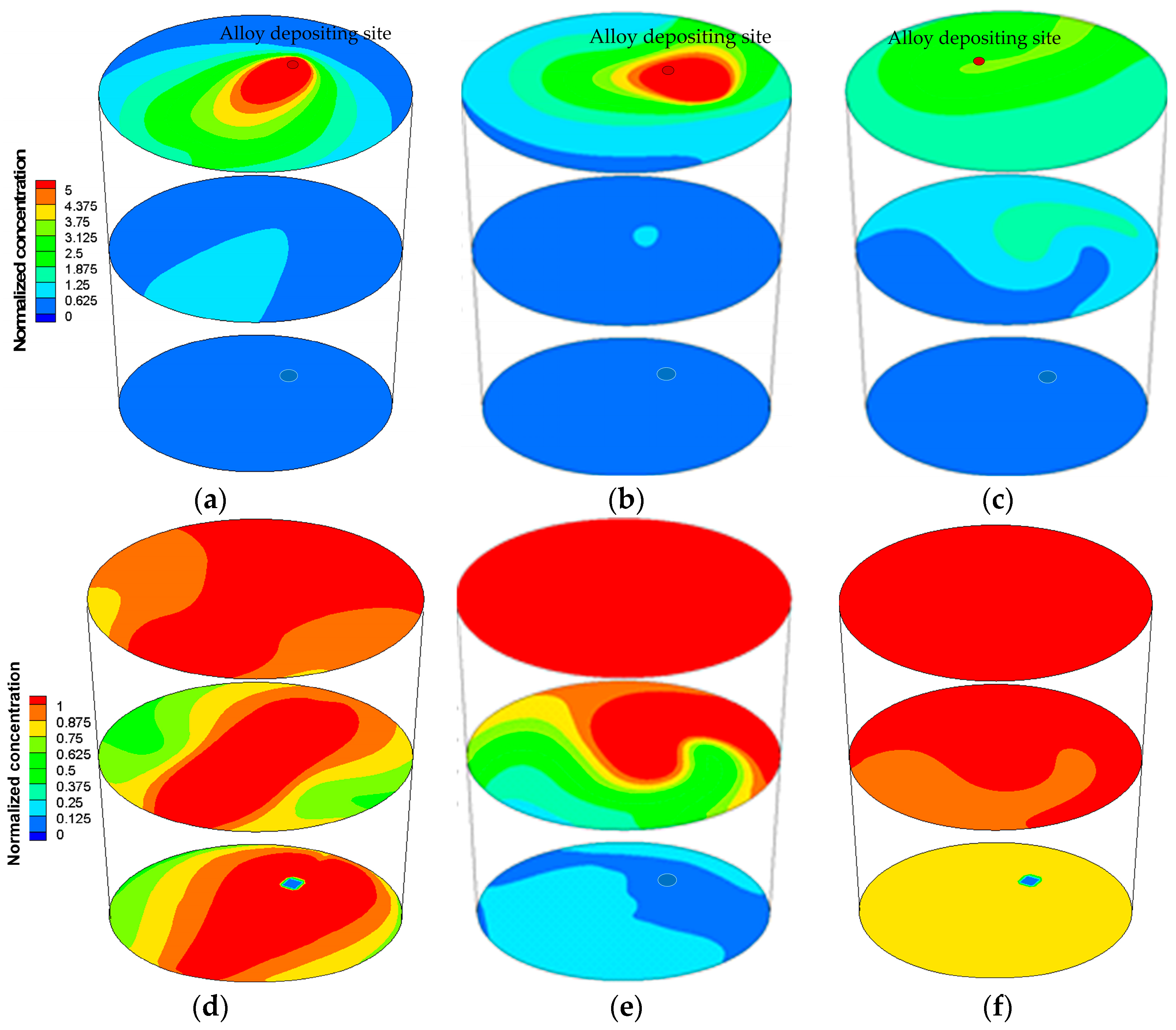
Figure 16.
Dead zone normalized concentration changes ((a,b) is non-EMS and bottom-rotating EMS (I = 600 A) with an alloy depositing site situating point (−1.3, 0, 3.732), respectively, and (c) is the bottom-rotating EMS (I = 600 A) with an alloy depositing site situating point (−0.38, 0.58, 3.732)).

Table 1.
Geometric parameters and operating conditions.
| Parameter | Value |
|---|---|
| Bottom diameter of ladle, m | 2.60 |
| Top diameter of ladle, m | 2.98 |
| Diameter of porous plug, m | 0.118 |
| Height of ladle, m | 3.732 |
| Height of stirrer, m | 0.3 |
| Turns of stirrer | 80 |
| Density of molten steel (ρl), kg·m−3 | 7020 |
| Viscosity of molten steel (μl), kg·m−1·s | 0.006 |
| Density of argon (ρg), kg·m−3 | 1.6228 |
| Viscosity of argon (μg), kg·m−1·s | 2.125 × 10⁻⁵ |
| Diameter of argon bubble (db), m | 0.004 |
| Specific heat capacity of molten steel (cp), J·kg−1·K | 434 |
| Thermal conductivity of molten steel (λ), W·m−1·K | 60.5 |
| Electric conductivity of molten steel (σ), S·m−1 | 7.14 × 10⁵ |
| Magnetic permeability (η), H·m−1 | 1.257 × 10⁻⁶ |
| Current intensity of EMS, A | 300, 600, 1200 |
| Operating frequency of EMS, Hz | 50 |
| Heat flux density of ladle wall, W/m2 | 11,702 |
| Heat flux density of ladle bottom, W/m2 | 8532 |
| Argon gas rate, L/min | 600 |
Table 2.
Characteristics of the different meshes and ux, uy, uz, and u errors.
| Case | A | B | C | D |
|---|---|---|---|---|
| Total cell number | 138,132 | 208,919 | 323,792 | 453,946 |
| Total node number | 145,310 | 217,920 | 355,880 | 469,800 |
| εux = ∑|uxi − uxD|/∑|uxD| | 0.0388 | 0.0110 | 0.0184 | - |
| εuy = ∑|uyi − uyD|/∑|uyD| | 0.0456 | 0.0367 | 0.0332 | - |
| εuz = ∑|uzi − uzD|/∑|uzD| | 0.0207 | 0.0189 | 0.0143 | - |
| εu = ∑|uiuD|/∑|uD| | 0.0614 | 0.0483 | 0.0290 | - |
Table 3.
The position of test points.
| Point | Coordinate (x, y, z) |
|---|---|
| 1 | (−0.4, 0.8, 0.5) |
| 2 | (0.3, −1, 0.6) |
| 3 | (0.3, 0.6, 0.7) |
| 4 | (−0.2, 0.6, 2) |
| 5 | (0, −0.8, 0.9) |
| 6 | (−0.52, −0.4, 3.3) |
| 7 | (0.8, −0.7, 0.6) |
| 8 | (0.08, −0.1, 3) |
| 9 | (1, −0.5, 0.6) |
| 10 | (0.4, −1, 0.55) |
© 2018 by the authors. Licensee MDPI, Basel, Switzerland. This article is an open access article distributed under the terms and conditions of the Creative Commons Attribution (CC BY) license (http://creativecommons.org/licenses/by/4.0/).
Share and Cite
MDPI and ACS Style
Li, Y.; Deng, A.; Li, H.; Yang, B.; Wang, E. Numerical Study on Flow, Temperature, and Concentration Distribution Features of Combined Gas and Bottom-Electromagnetic Stirring in a Ladle. Metals 2018, 8, 76. https://doi.org/10.3390/met8010076
AMA Style
Li Y, Deng A, Li H, Yang B, Wang E. Numerical Study on Flow, Temperature, and Concentration Distribution Features of Combined Gas and Bottom-Electromagnetic Stirring in a Ladle. Metals. 2018; 8(1):76. https://doi.org/10.3390/met8010076
Chicago/Turabian StyleLi, Yang, Anyuan Deng, Huan Li, Bin Yang, and Engang Wang. 2018. "Numerical Study on Flow, Temperature, and Concentration Distribution Features of Combined Gas and Bottom-Electromagnetic Stirring in a Ladle" Metals 8, no. 1: 76. https://doi.org/10.3390/met8010076
Note that from the first issue of 2016, this journal uses article numbers instead of page numbers. See further details here.