Online Surface Defect Identification of Cold Rolled Strips Based on Local Binary Pattern and Extreme Learning Machine


1
Collaborative Innovation Center of Steel Technology, University of Science and Technology Beijing, Beijing 100083, China
2
Quantitative Imaging Research Team, Data61, Commonwealth Scientific and Industrial Research Organization, Marsfield, NSW 2122, Australia
*
Author to whom correspondence should be addressed.
Metals 2018, 8(3), 197; https://doi.org/10.3390/met8030197
Submission received: 12 February 2018
/
Revised: 14 March 2018
/
Accepted: 17 March 2018
/
Published: 20 March 2018
Abstract
:In the production of cold-rolled strip, the strip surface may suffer from various defects which need to be detected and identified using an online inspection system. The system is equipped with high-speed and high-resolution cameras to acquire images from the moving strip surface. Features are then extracted from the images and are used as inputs of a pre-trained classifier to identify the type of defect. New types of defect often appear in production. At this point the pre-trained classifier needs to be quickly retrained and deployed in seconds to meet the requirement of the online identification of all defects in the environment of a continuous production line. Therefore, the method for extracting the image features and the training for the classification model should be automated and fast enough, normally within seconds. This paper presents our findings in investigating the computational and classification performance of various feature extraction methods and classification models for the strip surface defect identification. The methods include Scale Invariant Feature Transform (SIFT), Speeded Up Robust Features (SURF) and Local Binary Patterns (LBP). The classifiers we have assessed include Back Propagation (BP) neural network, Support Vector Machine (SVM) and Extreme Learning Machine (ELM). By comparing various combinations of different feature extraction and classification methods, our experiments show that the hybrid method of LBP for feature extraction and ELM for defect classification results in less training and identification time with higher classification accuracy, which satisfied online real-time identification.
1. Introduction
Cold rolled strip is a true all-round material in various products such as automobiles, electrical appliances, ships etc. With the rapid development of the economy, the demand for cold rolled strip increases year by year. In the production of cold rolled strip, various defects appear on the surface of the rolled strip due to various reasons such as issues from manufacturing technology, equipment etc. These defects not only affect the appearance of the products, but also degrade the performance of the products. To eliminate these defects, they should be detected at the first instance with a surface inspection system [1]. The detection system is machine vision-based, which has become the mainstream of all identification methods. Feature extraction and classification are the key steps of the machine vision method. The step “local feature extraction” has been widely used in machine vision for image recognition [2], image retrieval [3], image registration [4], image classification [5], image mosaicking [6]. Defects are caused for different reasons and appear in different types. Useful features are extracted from the surface images for the detection and classification of the defects on the surface. The cause of different types of defects can then be tracked and addressed.
New types of defects are often discovered in the production of cold rolled strip. To identify these new defects, the production line is normally suspended and then the classification model is retrained with added sample images for the new defect. If the re-training process takes a long time, the product will be impacted. Therefore, a classification model with fast training and identification algorithms is preferred. In the production line, workers change the rolls of a cold rolling mill when a coil of raw strip steel is run out. If the model retraining can be finished within the time of roll change, the classification model can be quickly adapted to the online real-time identification of new defects. This will avoid the suspension of the production.
In this paper, we will explore various options for the image feature extraction and classification and aim to find the best option for the fast identification of the defects with high classification accuracy and high computing performance for the training of the classification model.
There are several popular feature extraction methods, including Scale Invariant Feature Transform [7] (SIFT), Speeded Up Robust Feature [8] (SURF) and Local Binary Pattern [9] (LBP). Lowe proposed efficient SIFT algorithm to speed up feature extraction. Based on SIFT, Bay proposed more efficient SURF algorithm [8] to further speed up feature extraction. Ojala presented LBP algorithm [9], which is a redefinition of the grayscale values of the original image and a simple combination of histogram. Compared to SIFT and SURF, LBP has less computational complexity, leading to higher computing performance in feature extraction.
Literature has reported several popular classification methods, including Back Propagation neural networks [10] (BP), Support Vector Machine [11] (SVM) and Extreme Learning Machine [12] (ELM). The algorithms of BP neural networks are complicated and slow in training. BP neural network requires many iterations to compute weights [13] and it is easy for it to get stuck in a local minima. The identification of complex surface defects of cold rolled strip is a problem of multi-class classification, in which the classic SVM has some disadvantages [14]. ELM [15] (Extreme learning machine) is an improved algorithm based on single hidden layer feedforward neural networks. The only artificial parameter of ELM is the number of hidden layer nodes. Initial weights are randomly generated. ELM is fully automatically implemented without iterative tuning, and it is extremely fast compared to other traditional learning methods. Hence ELM is potentially a solution to satisfy the real-time requirement in online defect identification of cold rolled strip. This paper is organized as follows: Section 2 introduces the principle of LBP and ELM algorithms; Section 3 demonstrates the computing performance of LBP and ELM with comparison among several hybrid methods for the surface defect identification; Section 4 illustrates how the hybrid method of LBP and ELM can be adapted to identify a new defect with an online surface inspection case study; the conclusions are drawn in Section 5.
2. Principle of LBP (Local Binary Pattern) and ELM (Extreme Learning Machine) Algorithms
2.1. LBP Algorithm
2.1.1. Principle of the LBP
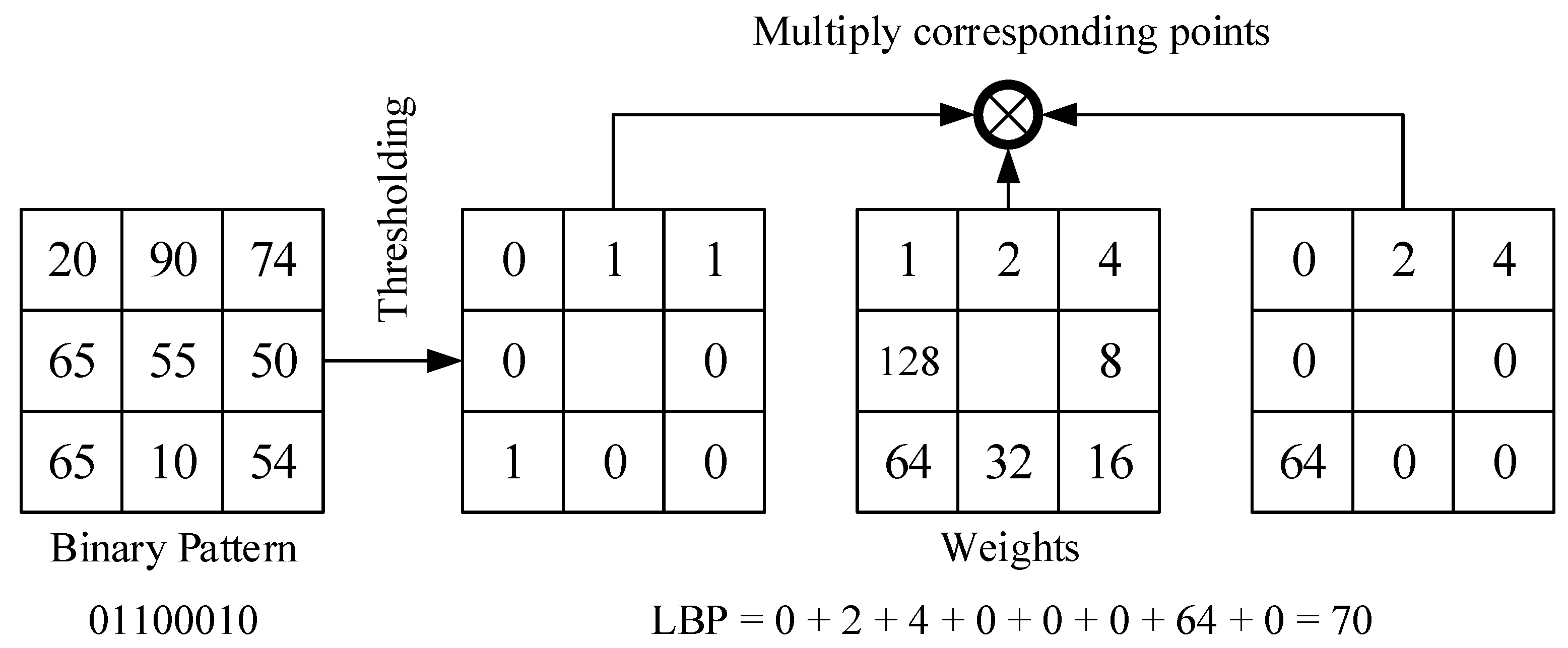
Local binary pattern (LBP) is a type of visual descriptor used for classification in computer vision.
As shown in Figure 1, the LBP feature vector, in its simplest form, is created as follows:
- (1)
- Compare each pixel in a cell with each of its 8 neighbors (on its top left, top right, right, bottom right, bottom, bottom left, left in order) clockwise.
- (2)
- If the value of the neighbor is larger than the value of the center pixel, write “0”, otherwise, write “1”. This generates an 8-digit binary number (usually converted to decimal for convenience).
- (3)
- Calculate the times of occurrence of each decimal number. Then a feature histogram is made (x-axis is decimal number; y-axis is the times of each decimal number occurring). This histogram can be seen as a 256-dimensional feature vector.
2.1.2. Improved LBP
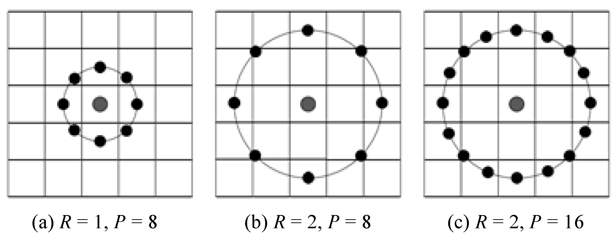
The original LBP operator has obvious limitation, namely its computation only covers a fixed area. To adapt to the changes of scale, LBP operator should be improved to address the limitation.
The improvement includes three aspects: firstly, the square neighborhood is changed into a circular one; secondly, its radius of the covered area is expanded from 1 to arbitrary size R [16]; thirdly, the number of sample points is changed to variant P. The improved LBP operator is shown in Figure 2.
The value of LBP patterns with the radius R and sample points P can be represented as . The encoding process of the improved LBP is similar to that of the basic LBP. Take as an example shown in Figure 3. First, 8 neighborhood points are selected as a circle. Then the gray value of selected points is calculated by bilinear interpolation. The procedures below are same as original LBP in Figure 1.
2.1.3. LBP Uniform Pattern
Set the number of sample points as P, then the maximum of LBP patterns is 2P. That is, the number of LBP patterns rises exponentially as P increases. When , the maximum of LBP patterns reaches , which is incredibly huge for data processing. Such a huge number of patterns will result in long calculation time. Furthermore, huge pattern numbers lead to a sparse feature vector and histogram that is not suitable to describe the feature of defect.
To solve these two problems, Ojala optimized the improved LBP operator and put forward the LBP uniform pattern [17]. This idea is motivated by the fact that some binary patterns occur more commonly in texture images than others [18]. The motivation for this idea is that some binary patterns are more common in texture images than the other. If the binary pattern contains up to two 0-1 or 1-0 transitions, these common binary patterns are called uniform patterns. For instance, 00000010 (2 transformations) is a uniform pattern, 0100100 (4 transformations) is not. Other uncommon binary patterns are called non-uniformed pattern if it contains more than 2 transitions. In LBP uniform pattern, the maximum of LBP patterns is , much smaller than 2P of the original LBP. In this paper, for , the number of LBP patterns decreases from 256 to 59.
In the LBP histogram calculation, the histogram has a separate bin for each uniform pattern, and all non-uniform patterns are assigned to a single bin. The length of the feature vector for one picture is reduced from 256 to 59 with a uniform pattern.
2.2. ELM Algorithm
2.2.1. The Theory of ELM
ELM is a popular machine-learning algorithm in recent years. The theory of the ELM algorithm is briefly introduced as below [15]. The model of ELM neural network is shown in Figure 4.
For N arbitrary distinct samples , where
The ELM with L hidden-layer nodes is mathematically described as
is activation function, using a common activation function such as sigmoid. is the weight vector connecting the ith hidden node and the input nodes, is the weight vector connecting the ith hidden node and the output node, is the bias parameter of the ith hidden node. The computation of ELM is to minimize the error between actual output and the ground truth of a training sample.
i.e., there exist , and , such that
The above N equations can be written compactly as , where
Our goal is to find specific , , such that
which is equivalent to minimizing the cost function
Unlike the approximation theories of traditional functions, which require the adjustment of input weights and hidden layer biases, input weights and hidden layer biases can be randomly assigned. The input weights and the hidden layer biases are in fact not tuned and the hidden layer output matrix H can actually remain unchanged. The learning process is simply equivalent to finding a solution of the linear system and the minimum norm least-squares solution of the above linear system is
where is the Moore–Penrose generalized inverse of matrix , and the norm of the solution is smallest and unique. Thus, ELM omits the process of adjusting input weights and hidden layer biases, only needs a generalized inverse, and this greatly improves the speed for training the ELM neural network.
2.2.2. The Classification Strategies of ELM
Maximum Strategy
Using an N-dimensional vector of sample features, a trained ELM can produce an output of an M-dimensional vector, where M is the number of classes for the classification. In this work, the samples of cold rolled strip are from 4 categories of defects. Therefore, the output of ELM is a four-dimensional vector in response to each input sample . For example, a specific sample belongs to defect I, its output vector is . If it belongs to defect II, then is , and so on. Each dimension of this vector varies between −1 and 1, which means that each element of this vector represents the probability of each defect category. For instance, if the output is , the first element of the vector is the largest, thus the defect category is I. The maximum strategy is most effective when all defect categories are known, and their training samples are used in the training stage of ELM.
If the output is a vector such as , according to the maximum strategy, the 4th element of the vector is the largest, thus the defect belongs to Category IV. However, all elements of the output vector are negative. This means that this actual defect may belong to none of any known categories. In this case, the maximum strategy is not applicable.
Real-Time Identification Strategy
In the production of cold rolled strip, from time to time, a new category of defect may be observed. To monitor these new categories of defects, we proposed a real-time identification strategy as described below.
The procedure for determining a new category of defect is described below:
- (1)
- Set a threshold ,
- (2)
- Find ,
- (3)
- If , the defect is to be classified into the jth known category, otherwise the defect sample should be classified as “unknown”.
For instance, if we set , and if an output vector is , thus . This satisfies , so this defect belongs to Category IV (). For an output vector such as , , which does not satisfy , so the defect should be classified as “unknown”.
3. Experiment and Analysis of Defect Identification
In this section, we present our experimental results by comparing the performance of ELM and other algorithms for surface defect identification of cold rolled strip.
3.1. General Design of the Experiment
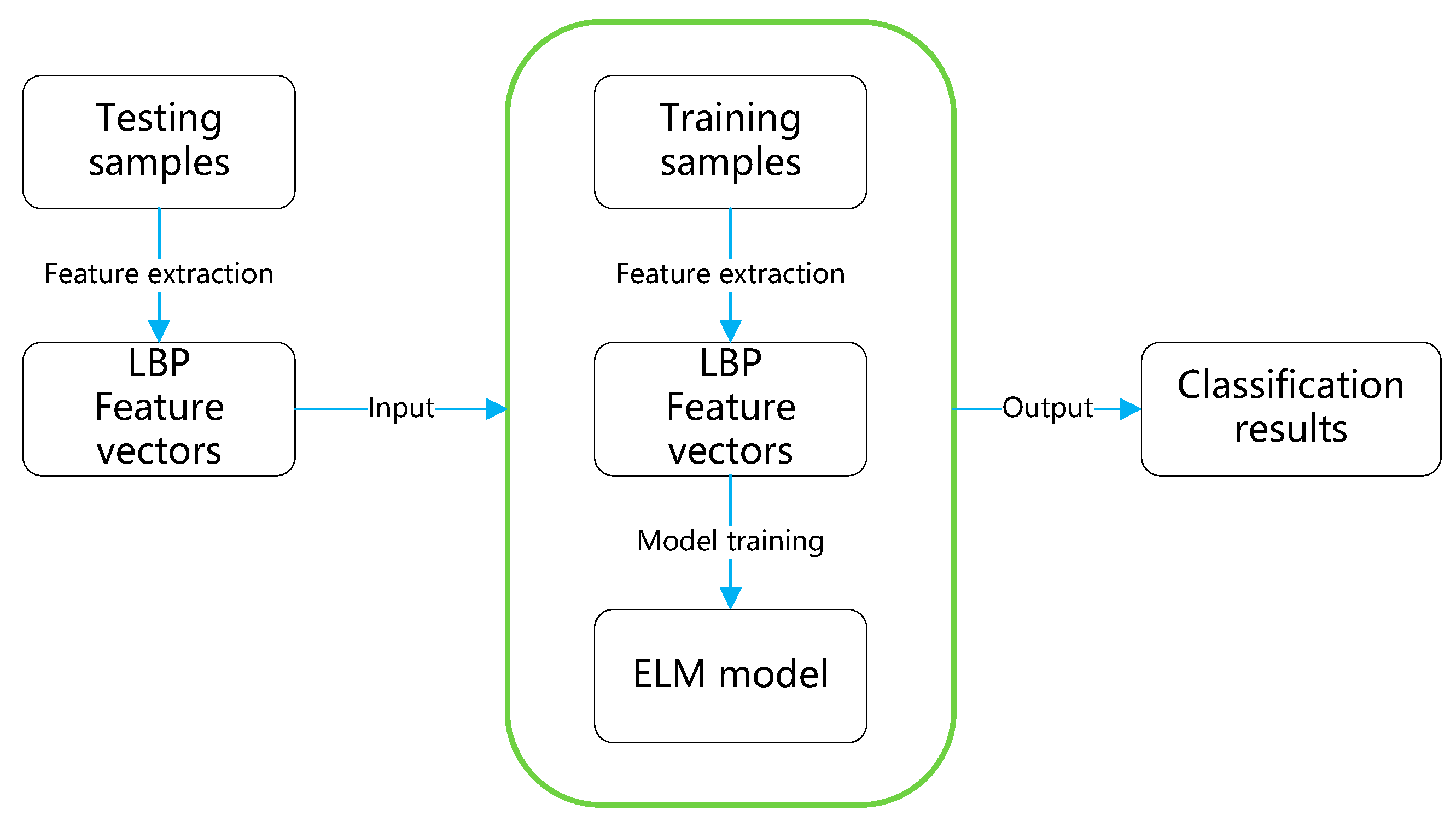
The flowchart of the experiment for defect identification is shown in Figure 5. In the experiment, all the samples are divided into training set and testing set. The training set includes 4 categories, 1348 samples in total. The same is true for the testing set, it includes 4 categories, and 1130 samples in total. Specific distribution of samples is shown in Table 1. We used cross-validation method to train the model by splitting the samples into m shares to train the model and using one share each time.
3.2. Feature Extraction Using LBP
3.2.1. Image Processing with LBP Operator
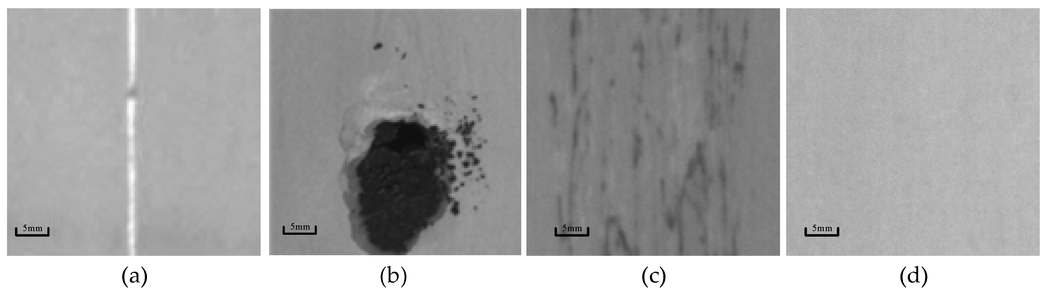
There are various types of defects on the surface of cold rolled strip. Among these types of defects, scratches, slags, and peels have significant negative impact on the quality of the strip; furthermore, these defects are the most common ones occurred in the production process. Therefore, these three defects are the main focus for defect identification.
As has been mentioned in Section 2, LBP algorithm can be used to characterize the texture of images by comparing the grayscale between pixels. It is a linear method for removing light effect by extracting local features. LBP algorithm does not change the position and number of pixels in an image, therefore it does not change the size of the image.
Figure 6 shows some defect images including scratches, slags, peels, and an image with no defects. Figure 7 shows the corresponding images after applying LBP for extracting features. As shown in these two figures, LBP method clearly preserves the texture details of the original images, while removing the effect of uneven lighting.
3.2.2. Statistical Analysis and Dimension Reduction of LBP Images
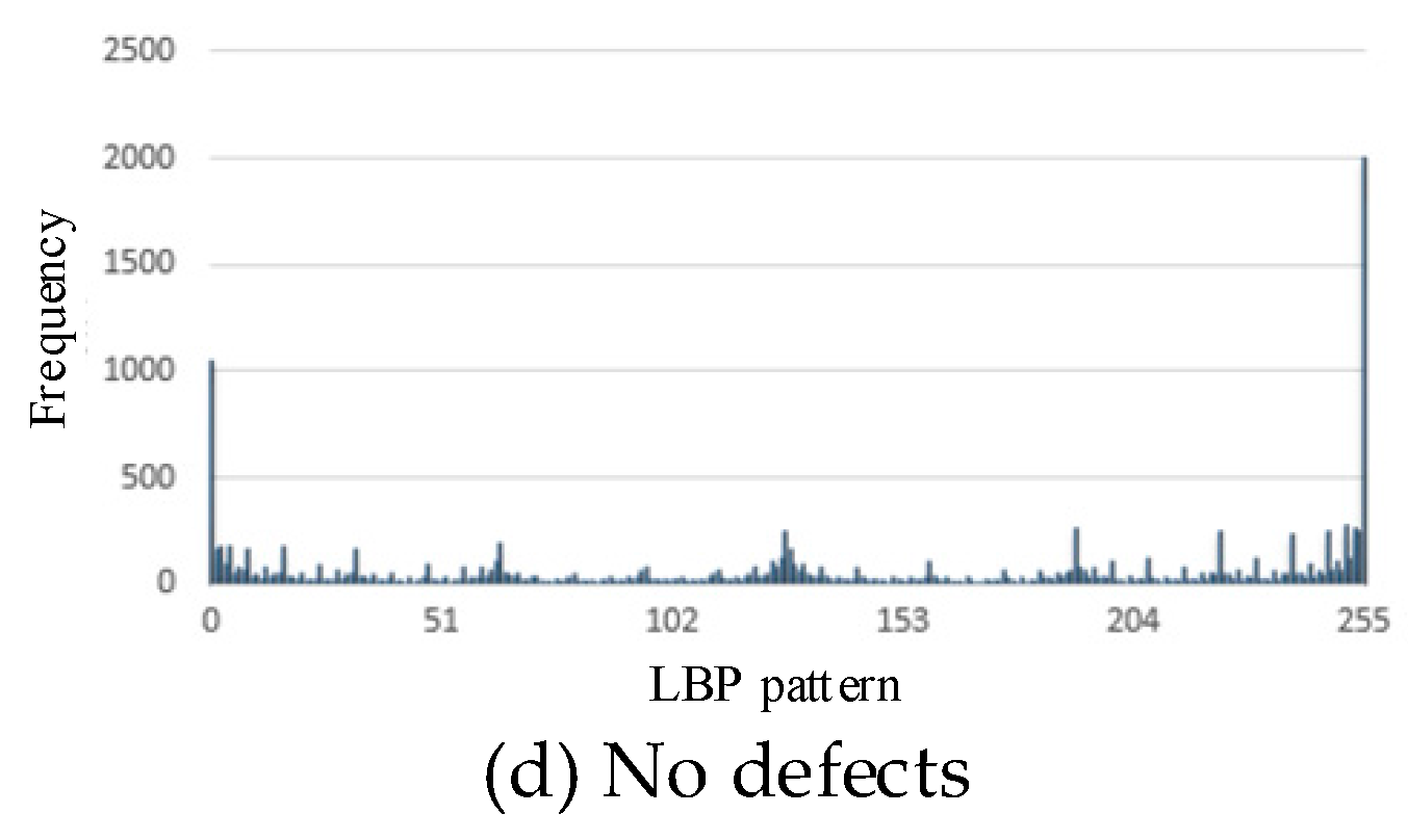
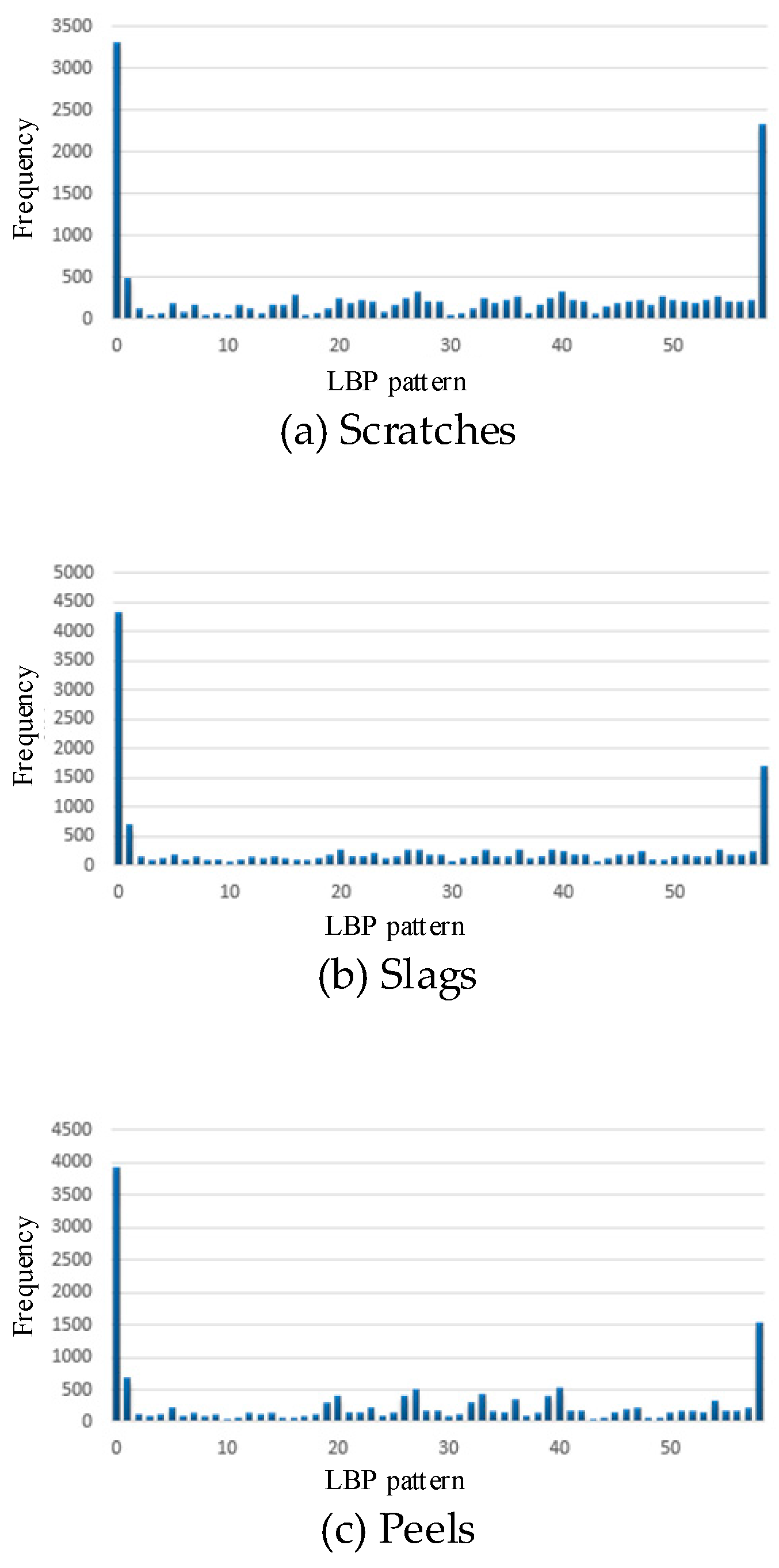
This section presents the histogram of LBP patterns for different types of defects. Images with 256-level grayscales are used to show the distribution of LBP patterns, that is, the frequency of different gray levels in a defect image. The LBP pattern is a one-dimensional vector containing 256 eigenvalues, in which the kth eigenvalue represents the occurrence rate of the kth LBP pattern in the whole image.
Figure 8 shows the histogram of LBP patterns for the above three types of defects and the one without defects. As shown in Figure 8, the histograms of LBP patterns for different defects are quite different. Therefore, the LBP patterns for different defects can be used to train classification models for defect identification.
LBP uniform pattern described in Section 2 can be used for dimension reduction for the LBP patterns. We used the LBP uniform pattern and reduced the dimension of LBP patterns from 256 to 59.
Figure 9 shows the 59-dimensional histogram of LBP patterns after the dimension reduction. The dimension reduction has two advantages: (1) remove low frequency LBP especially noises, and (2) reduce the computation in training classifiers for the defect identification and therefore reduce the training time.
3.2.3. A Comparison of Computing Performance among LBP and Other Feature Extraction Methods
Apart from LBP, the most common local feature-extraction descriptor is SIFT and SURF. SIFT can improve the computing speed based on SURF. They both perform well on feature extraction, compared with LBP. However, the computation complexity and cost of SIFT and SURF are high, so they are not suitable for the real-time applications. The following table shows the comparison of computation time among LBP, SIFT and SURF. As shown in Table 2, LBP performs the best in terms of computation cost.
3.3. Model Training Using ELM
3.3.1. Optimization of the Number of Hidden-Nodes
The number of hidden nodes has great impact on the performance of computation and classification of the defects. If the number is too large, it will cause an over-fitting problem that reduces the generalization ability of ELM. If it is too small, it may lead to an under-fitting problem that reduces the acquisition of all features of the training set.
We select the number of hidden nodes based on the following principle. (1) Refer to the empirical number of the ELM method; (2) Compute the number in I-ELM method; and (3) Depend on the accuracy of cross-validation test.
Figure 10 shows the accuracy of the cross-validation test with different hidden-nodes numbers. When the node number is 50, the identification achieves the highest accuracy. Therefore, we select 50 as the hidden-node number.
3.3.2. Comparison of Training Time between ELM and Other Models
ELM omits the process of adjusting input weights and hidden layer biases, this greatly saves the training time. Table 3 shows the comparison of training time among ELM and other models. For more accurate comparison of training time, we set 50 hidden nodes for BP neural network as well as linear kernel for SVM. The comparison shows ELM takes much less time to train than the others.
3.4. Defect Identification Using ELM
This section reports the classification results of various defects using ELM. We use a confusion matrix to show the actual and classified defect classes.
3.4.1. Analysis on the Result of Defect Identification
We used 1130 sample defect images for testing the ELM classifier, including 216 images for scratch, 100 images for slag, 302 images for peel, 512 samples with no defects. After extracting features and reducing dimensions for each sample image, we obtained a 256-dimensional and a 59-dimensional feature vector for classification. The confusion matrices for the classification using a 59-dimensional feature vector and 256-dimensional feature vector are shown in Table 4 and Table 5, respectively.
As shown in Table 4 and Table 5, the classification accuracy for the defects of scratch and peel are about 95%. This is because these two defect types have distinguishing features and many samples for training. The classification accuracy for the defect of slag is about 89%, which is less than those for other defect types. This is because the image features of these types of defect are less perceptible than those for other defects. It is worth mentioning that all images with no defects are classified correctly using either their 256-dimensional feature vectors or 59-dimensional feature vectors. This is because the image features with no defects are distinct, and there are lots of sample images for training.
3.4.2. Comparison of the Performance of Computation and Classification among ELM and Other Models
To compare the performance of ELM and other classification models, we have conducted experiments and populated the experiment results in Table 6 to show both the computation and classification performance. From Table 6, we can see that:
- (1)
- BP neural network is not performing well in terms of classification accuracy when the training dataset is small;
- (2)
- The classification accuracy of SVM is high, however, it takes long time to identify the defects.
- (3)
- LBP + ELM outperforms others, it can achieve higher classification accuracy with less training time than other models in Table 6.
4. Experiment and Analysis of Online Monitoring with New Types of Defects
In the production of cold rolled strip, new types of defects often appear due to various types of equipment malfunctions. In this case, the pre-trained defect classification model is no longer suitable for identifying these new defect types. This will lead to misclassification of the defects and has negative impact on the product quality. By accurately identifying the defect types, operators can take actions accordingly to mitigate the negative impact of the defects. Therefore, it is important to address the problem of identifying new types of defects.
In this section, an online monitoring experiment has been carried out. ELM has been used for the classification of new types of defects.
4.1. Design of the Experiment
The primary purpose of online monitoring is to improve identification reliability. That is, when new types of defects appear, the classification model can quickly sense the defects and properly adjust itself to identify them.
Figure 11 shows the flowchart of the defect identification process. First, we train ELM using images of known defect types. Then ELM is used to identify the defect types of images captured from the production line. This works well.
If new types of defects are present, the images with new types of defects will be captured and saved for manual classification. When the images with new defect types accumulate to a certain number, they will be added to the training set. Then the training set is used to retrain the model. As aforementioned, ELM can be trained in seconds and the re-trained model can be used for online monitoring immediately.
4.2. Experiment Process
4.2.1. Training of ELM
ELM was initially trained with four typical defect types. These four defect types are shown in Figure 12.
The number of training samples for each defect type is shown in Table 7. These four types of defects are the most common and representative ones in the production of cold rolled strip. The number of training samples in Table 7 is smaller than that in Section 3 (shown in Table 1). This is because the samples used in this experiment have more representative features than those in Table 1. Therefore, even the training set is smaller in this experiment, high classification rate can also be achieved.
For more accurate comparison of experimental results, we set the number of nodes in the hidden layer to 50 which is the same as used in the experiment in Section 3.
4.2.2. Defect Identification Using ELM
After training ELM, it is used for the defect classification. The trained model will output a 4-dimensional vector corresponding to the four types of defects.
In Section 2.2, two classification strategies of ELM are proposed, that is maximum strategy and real-time identification strategy. With the experiment in Section 3, the maximum strategy is used. In that experiment, all testing samples belong to the four known types, so each image sample will be classified into one of the four defect types. In this section, the real-time identification strategy is used to address the problem coming with new defect types. With the real-time identification strategy, a testing sample will be classified into one of four defect classes only when the corresponding one of the four elements in the output vector is greater than or equal to the preset threshold .
To determine a proper value for the threshold, we have conducted cross-validation. All samples in the training set are with known defect types. When plotting the curve of classification accuracy against different threshold values, we observe that the classification accuracy drops significantly when the threshold ε approaches the value of −0.1. As shown in Figure 13, the inflection point appears when the threshold ε is equal to −0.1. Therefore, we use −0.1 as the value of the threshold ε in this experiment. That is, if the maximum value of the elements in the output vector is less than −0.1, this test sample should be classified as “unknown”.
Table 8 shows the confusion matrix obtained by using the trained ELM to classify the testing dataset. As shown in the table, the average classification accuracy is about 92%, slightly less than that shown in Section 3.4.1 (Table 5). This may be caused by the smaller sample size of training set. Another observation is that several samples are classified as unknown defect types due to the change of classification strategy. The proportion of these samples is about 1.1%. This is still acceptable. When the “unknown” types of defects appear more frequently, we have to re-train ELM, and this is described in the following section.
4.2.3. Re-Training ELM with New Types of Defects
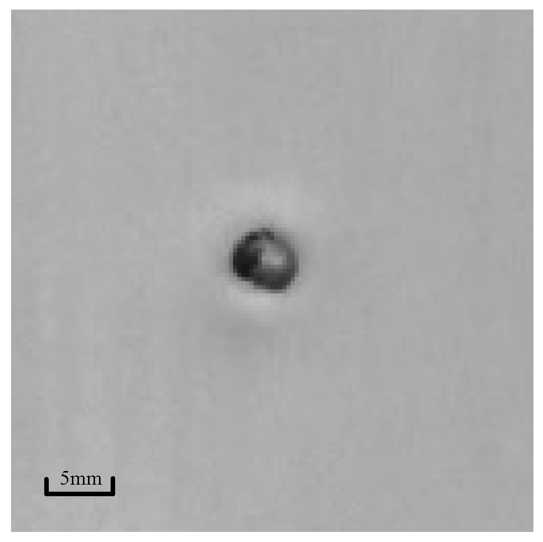
With the new types of defects being detected, we have manually identified that the new defect type is “pore”, as shown in Figure 14. Over time, more “unknown” types of defects are identified. Table 9 shows the confusion matrix with the additional defects of “pores”.
As shown in Table 9, the average classification accuracy drops to about 87.6%, lower than the average accuracy of 92% shown in Table 5. This shows that a small number of samples of “unknown” types of defects has little effect on average classification accuracy. However, when lots of unknown defects are present, ELM should be re-trained with the “unknown” defect types added into the training dataset.
Before adding the “unknown” types of defect samples into the training dataset, we need to manually label them. The re-trained ELM can then be used to replace the old model for defect classification. Table 10 shows the new confusion matrix using the retrained ELM. As shown in the table, the proportion of unknown defects has significantly dropped when using the retrained ELM for classification. We notice that the classification accuracy for the new defect type “pore” is not high. This is because the number of training samples for this type of defect is not large enough. This means that the re-training of the classification model should happen only when sufficient number of unknown types of defects appear.
5. Conclusions
To detect and identify various types of surface defects of cold rolled strip, we have developed an online monitoring system. The system is capable of extracting features of the surface images acquired from the cold rolling production line, and then using the features as input of the ELM classifier. In the production environment, for yield and quality assurance, the model should be quick enough in feature extraction and defect identification based on satisfactory classification accuracy. For potential new defects, fast classifier re-training and satisfactory classification accuracy of re-trained classifier are both necessary.
This paper has explored different feature extraction methods (SIFT, SURF, LBP) and various classifiers (BP, SVM, ELM) to find the fastest combination method with satisfactory classification accuracy. After getting the best combination method, this paper also explored its re-training time and classification accuracy when dealing with new types of defects.
The conclusions from our study are as follows:
- (1)
- LBP is faster in extracting features than traditional methods SIFT and SURF.
- (2)
- ELM can be trained faster than traditional classification method BP and SVM for its simple algorithm.
- (3)
- When dealing with known types of defects, the hybrid LBP + ELM method is more efficient than other combination methods with less training time (865 ms on 1348 samples), classification time (15 ms per sample), and higher classification accuracy (more than 96%).
- (4)
- When dealing with new types of defects, in most cases of production line environment, the samples of new types of defects will be less than training samples in experiment (1348), so the retraining time will be less than 1 s. The retrained classifier also has satisfactory classification accuracy (more than 86%).
On accounts of the satisfactory classification time, re-training time and classification accuracy on major known pre-trained defects and minor new defects in production environment, the hybrid LBP + ELM method satisfy the demand of real-time online defect monitoring system for continuous cold rolling process.
Acknowledgments
This work is sponsored by The National Natural Science Foundation of China (No. 51674031). The authors are indebted to the Collaborative Innovation Center of Steel Technology (CICST), the University of Science and Technology Beijing (USTB), Quantitative Imaging Research Team (QIRT) and Commonwealth Scientific and Industrial Research Organization (CSIRO) for the development infrastructure and financial support.
Author Contributions
Yang Liu conceived, designed and designed the experiments; Ke Xu and Dadong Wang contributed experiment data, materials and experiment equipments; Yang Liu and Ke Xu analyzed the data; Yang Liu wrote the paper; Ke Xu and Dadong Wang revised the paper.
Conflicts of Interest
The authors declare no conflict of interest.
References
- Xu, K.; Liu, S.; Ai, Y. Application of Shearlet Transform to Classification of Surface Defects for Metals. Image Vis. Comput. 2015, 35, 23–30. [Google Scholar] [CrossRef]
- Kawano, Y.; Yanai, K. Food image recognition with deep convolutional features. In Proceedings of the 2014 ACM International Joint Conference on Pervasive and Ubiquitous Computing: Adjunct Publication, Seattle, WA, USA, 13–17 September 2014; ACM: New York, NY, USA, 2014; pp. 589–593. [Google Scholar]
- Yue-Hei Ng, J.; Yang, F.; Davis, L.S. Exploiting local features from deep networks for image retrieval. In Proceedings of the IEEE Conference on Computer Vision and Pattern Recognition Workshops, Boston, MA, USA, 8–10 June 2015; pp. 53–61. [Google Scholar]
- Mohanaiah, P.; Sathyanarayana, P.; GuruKumar, L. Image texture feature extraction using GLCM approach. Int. J. Sci. Res. Publ. 2013, 3, 1. [Google Scholar]
- Romero, A.; Gatta, C.; Camps-valls, G. Unsupervised Deep Feature Extraction for Remote Sensing Image Classification. IEEE Trans. Geosci. Remote Sens. 2016, 54, 1349–1362. [Google Scholar] [CrossRef]
- Bheda, D.; Joshi, M.; Agrawal, V. A study on features extraction techniques for image mosaicing. Int. J. Innov. Res. Comput. Commun. Eng. 2014, 2, 3432–3437. [Google Scholar]
- Li, Y.; Liu, W.; Li, X.; Huang, Q.; Li, X. GA-SIFT: A new scale invariant feature transform for multispectral image using geometric algebra. Inf. Sci. 2014, 281, 559–572. [Google Scholar] [CrossRef]
- Bay, H.; Ess, A.; Tuytelaars, T.; Van Gool, L. Speeded-up Robust Features (surf). Comput. Vis. Image Underst. 2008, 110, 346–359. [Google Scholar] [CrossRef]
- Ojala, T.; Pietikäinen, M.; Harwood, D. A Comparative Study of Texture Measures with Classification Based on Featured Distributions. Pattern Recognit. 1996, 29, 51–59. [Google Scholar] [CrossRef]
- Hecht-Nielsen, R. Theory of the backpropagation neural network. Neural Netw. 1988, 1 (Suppl. S1), 445–448. [Google Scholar] [CrossRef]
- Jiang, J.; Song, C.; Wu, C.; Marchese, M.; Liang, Y. Support vector machine regression algorithm based on chunking incremental learning. In Proceedings of the International Conference on Computational Science, Reading, UK, 28–31 May 2006; pp. 547–554. [Google Scholar]
- Huang, G.; Zhu, Q.; Siew, C. Extreme Learning Machine: Theory and Applications. Neurocomputing 2006, 70, 489–501. [Google Scholar] [CrossRef]
- Yu, D.; Deng, L. Efficient and Effective Algorithms for Training Single-hidden-layer Neural Networks. Pattern Recognit. Lett. 2012, 33, 554–558. [Google Scholar] [CrossRef]
- Hu, J.; Li, D.; Duan, Q.; Han, Y.; Chen, G.; Si, X. Fish species classification by color, texture and multi-class support vector machine using computer vision. Comput. Electron. Agric. 2012, 88, 133–140. [Google Scholar] [CrossRef]
- Huang, G.B.; Zhu, Q.Y.; Siew, C.K. Extreme learning machine: A new learning scheme of feedforward neural networks. In Proceedings of the 2004 IEEE International Joint Conference on Neural Networks, Budapest, Hungary, 25–29 July 2004; Volume 2, pp. 985–990. [Google Scholar]
- Mohamed, A.A.; Yampolskiy, R.V. An improved LBP algorithm for avatar face recognition. In Proceedings of the 2011 XXIII International Symposium on Information, Communication and Automation Technologies (ICAT), Sarajevo, Bosnia and Herzegovina, 27–29 October 2011; pp. 1–5. [Google Scholar]
- Nanni, L.; Lumini, A.; Brahnam, S. Survey on LBP Based Texture Descriptors for Image Classification. Expert Syst. Appl. 2012, 39, 3634–3641. [Google Scholar] [CrossRef]
- Shan, C. Learning Local Binary Patterns for Gender Classification on Real-world Face Images. Pattern Recognit. Lett. 2012, 33, 431–437. [Google Scholar] [CrossRef]
Figure 1.
Principle and encoding process of the LBP (Local Binary Pattern).

Figure 2.
Principle of improved LBP.

Figure 3.
Encoding process of the improved .
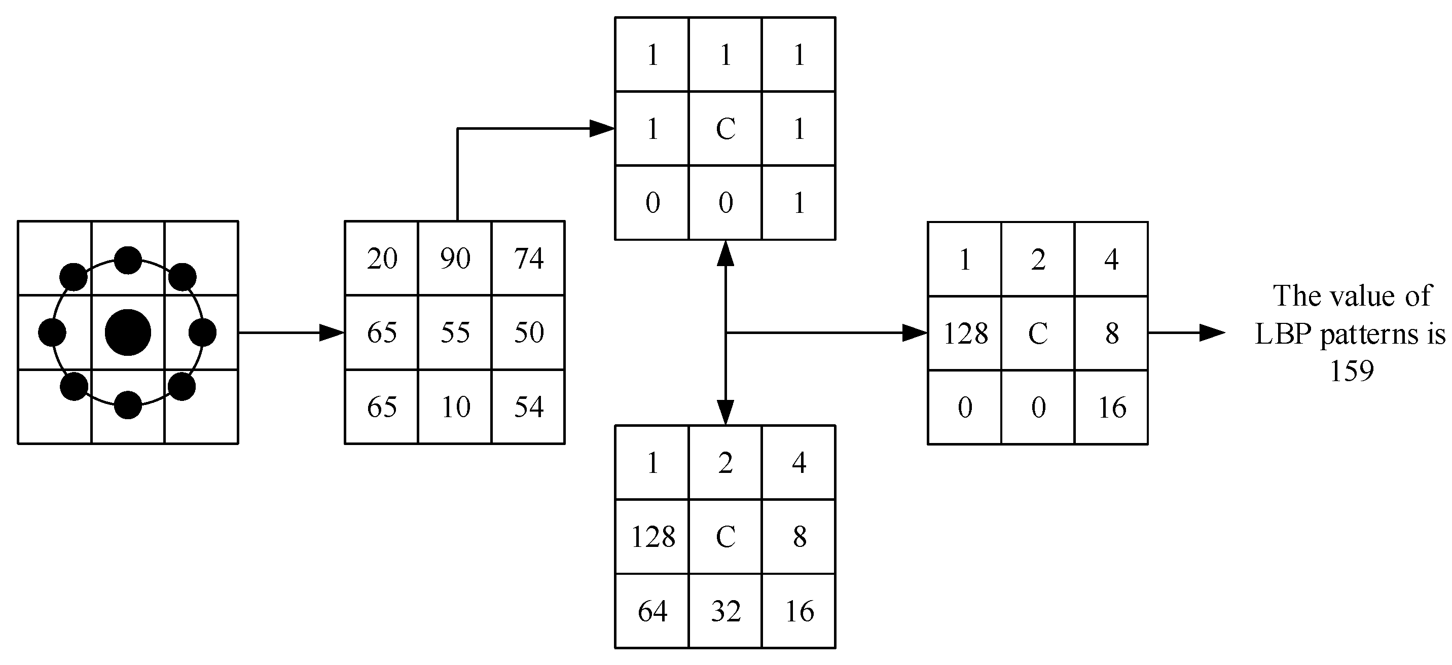
Figure 4.
Model of ELM neural network.
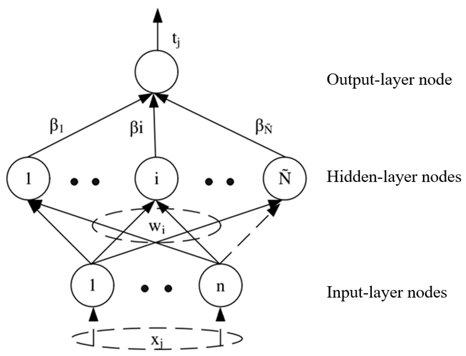
Figure 5.
Flowchart of the experiment.

Figure 6.
Original defect images: scratches (a), slags (b), peels (c), no defects (d).
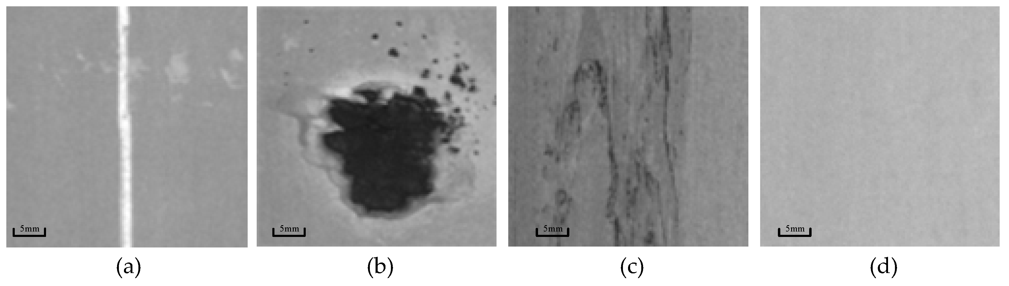
Figure 7.
The images after applying LBP feature extraction: scratches (a), slags (b), peels (c), no defects (d).
Figure 7.
The images after applying LBP feature extraction: scratches (a), slags (b), peels (c), no defects (d).
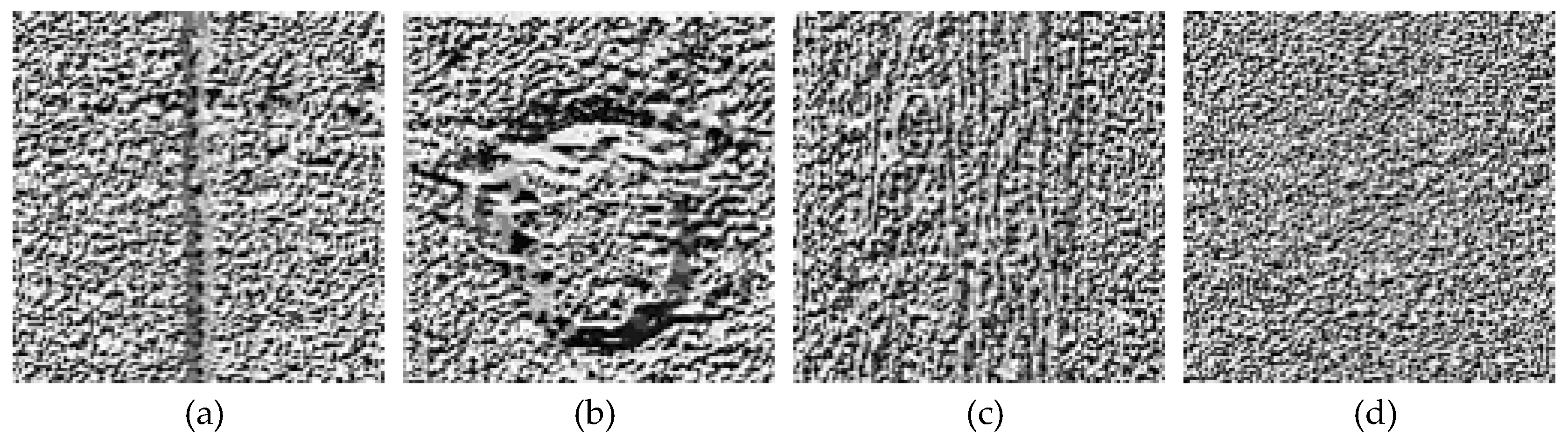
Figure 8.
The 256-dimensionial histogram of LBP patterns: scratches (a), slags (b), peels (c), no defects (d).
Figure 8.
The 256-dimensionial histogram of LBP patterns: scratches (a), slags (b), peels (c), no defects (d).


Figure 9.
59-dimensional histogram of LBP patterns: scratches (a), slags (b), peels (c), no defects (d).
Figure 9.
59-dimensional histogram of LBP patterns: scratches (a), slags (b), peels (c), no defects (d).

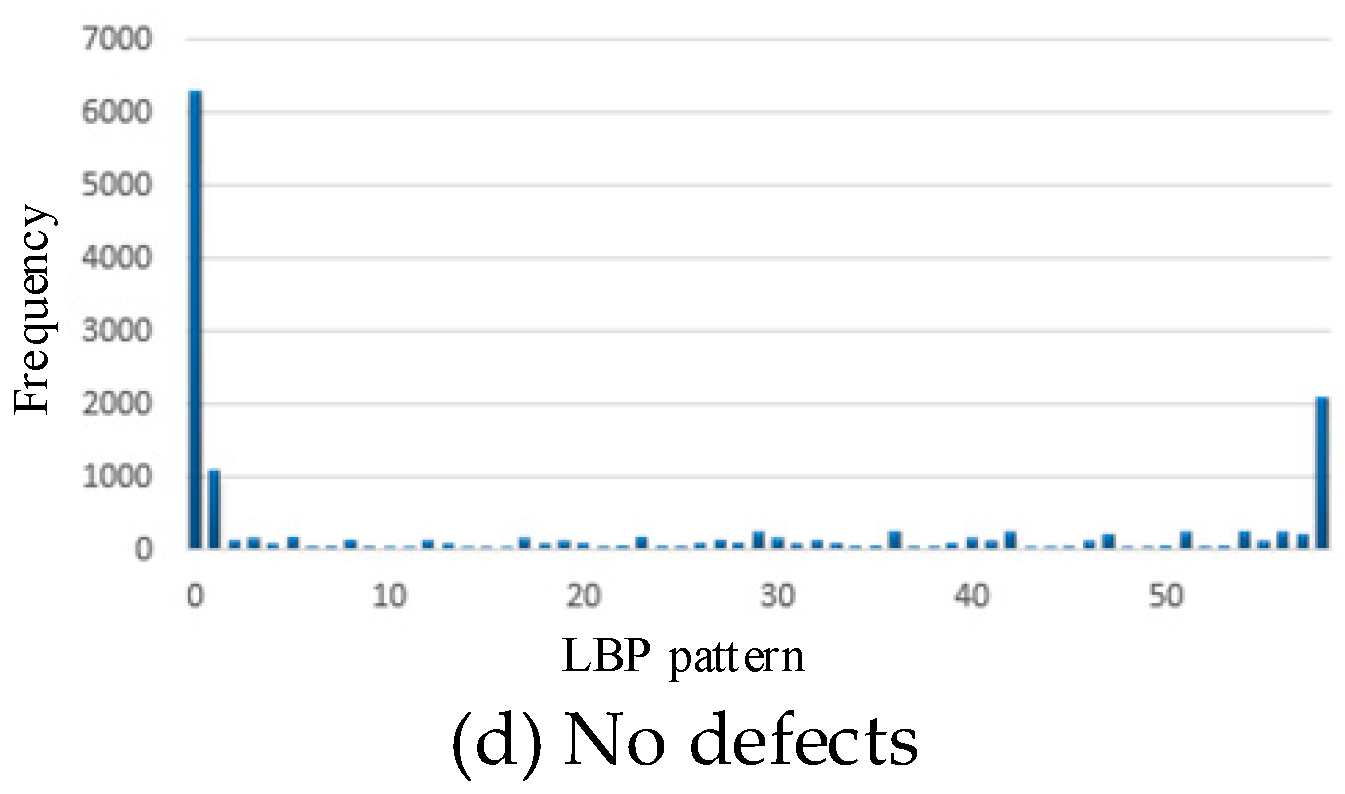
Figure 10.
Accuracy of cross-validation test with different hidden-nodes numbers.
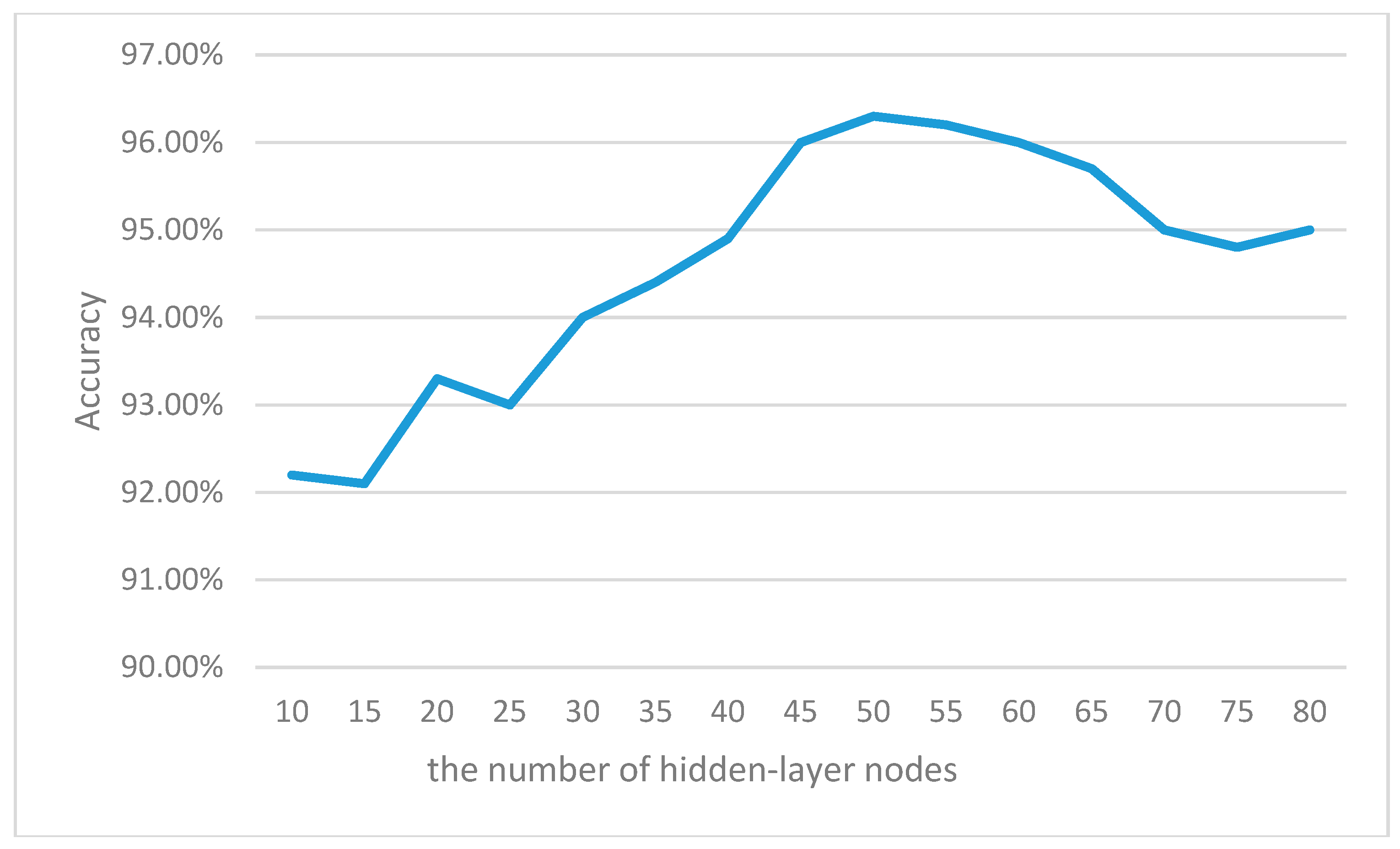
Figure 11.
Flowchart of the online monitoring system.
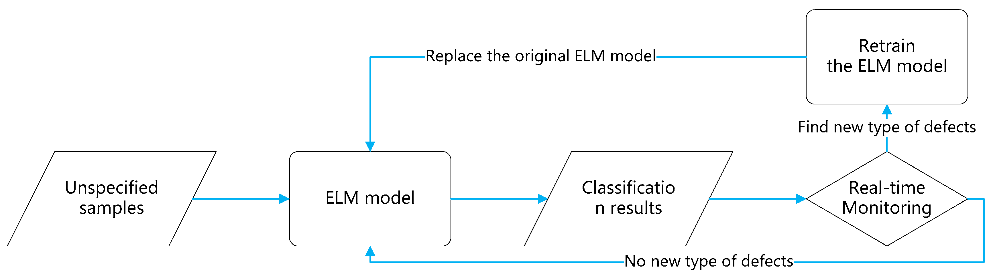
Figure 12.
Four defect types: scratches (a), slags (b), peels (c), no defects (d).

Figure 13.
Classification accuracy changes with different threshold values.
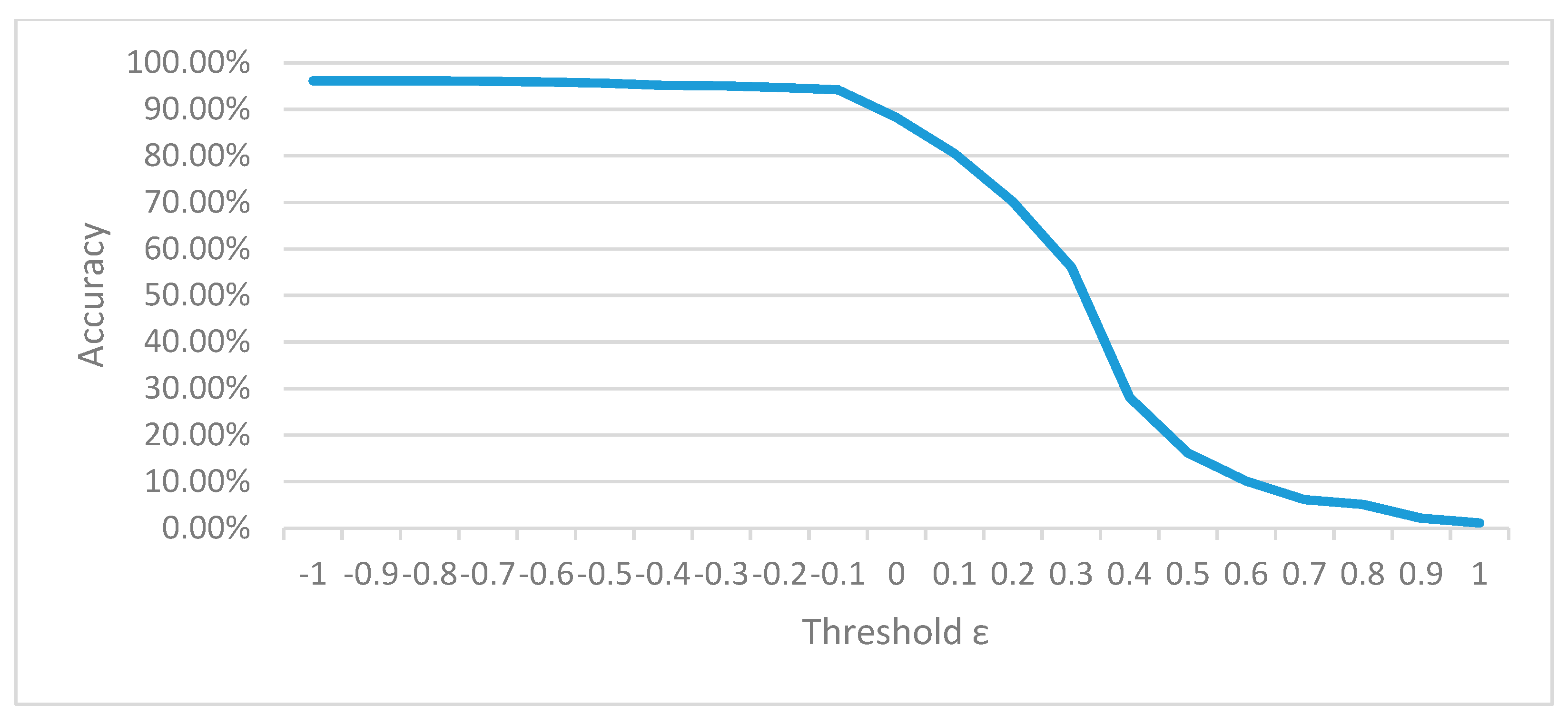
Figure 14.
Pores defect.


Table 1.
The number of training and testing samples.
| Defect Type | Number of Training Samples | Number of Testing Samples |
|---|---|---|
| Scratch | 296 | 216 |
| Slag | 178 | 100 |
| Peel | 362 | 302 |
| No defect | 512 | 512 |
Table 2.
Comparison of average computation time among LBP, SIFT and SURF.
| Method | Sample Size (Pixels) (0.3 mm/Pixel) | Dimensions | Computation Time (ms) |
|---|---|---|---|
| LBP | 128 × 128 | 256 | 15 |
| LBP | 128 × 128 | 59 (After dimension reduction) | 15 |
| SIFT | 128 × 128 | 128 × number of features | 72 |
| SURF | 128 × 128 | 64 × number of features | 22 |
Table 3.
Comparison of training time among ELM and other models.
| Learning Model | Sample Size | Feature Dimensions | Parameters | Training Time (ms) |
|---|---|---|---|---|
| BP | 1348 | 256 | 50 hidden nodes | 153,354 |
| BP | 1348 | 59 | 50 hidden nodes | 41,017 |
| SVM | 1348 | 256 | Linear Kernel | 6338 |
| SVM | 1348 | 59 | Linear Kernel | 6137 |
| ELM | 1348 | 256 | 50 hidden nodes | 2059 |
| ELM | 1348 | 59 | 50 hidden nodes | 865 |
Table 4.
Confusion matrix using ELM with 256-dimensional feature vectors.
| Defect Type | Scratch | Slag | Peel | No Defect | Correctly Classified | Sample Number | Classification Accuracy |
|---|---|---|---|---|---|---|---|
| Scratch | 204 | 0 | 2 | 10 | 204 | 216 | 94.44% |
| Slag | 5 | 85 | 6 | 4 | 85 | 100 | 85.00% |
| Peel | 6 | 5 | 281 | 10 | 281 | 302 | 93.05% |
| No defect | 0 | 3 | 4 | 505 | 505 | 512 | 98.63% |
| Total | 215 | 93 | 293 | 529 | 1075 | 1130 | 95.13% |
Table 5.
Confusion matrix using ELM with 59-dimensional feature vectors.
| Defect Type | Scratch | Slag | Peel | No Defect | Correctly Classified | Sample Number | Classification Rate |
|---|---|---|---|---|---|---|---|
| Scratch | 206 | 4 | 2 | 4 | 206 | 216 | 95.37% |
| Slag | 1 | 89 | 6 | 4 | 89 | 100 | 89.00% |
| Peel | 3 | 5 | 289 | 5 | 289 | 302 | 95.70% |
| No defect | 0 | 0 | 0 | 512 | 512 | 512 | 100.00% |
| Total | 210 | 98 | 297 | 525 | 1096 | 1130 | 96.99% |
Table 6.
Comparison of the computation and classification performance among ELM and other methods.
| Method | Average Classification Accuracy | Feature Dimensions | Classification Time (ms Per Sample) |
|---|---|---|---|
| SURF + SVM | 90.57% | 64 × number of features | 138 |
| LBP + BP | 69.71% | 256 | 33 |
| LBP + BP | 82.45% | 59 | 21 |
| LBP + SVM | 94.47% | 256 | 47 |
| LBP + SVM | 95.01% | 59 | 43 |
| LBP + ELM | 95.13% | 256 | 17 |
| LBP + ELM | 96.99% | 59 | 15 |
Table 7.
The number of training samples for each defect type.
| Defect Type | Number of Training Samples |
|---|---|
| Scratch | 160 |
| Slag | 80 |
| Peel | 200 |
| No significant defect | 300 |
Table 8.
Confusion matrix with unknown defect type.
| Defect Type | Scratch | Slag | Peel | No Defect | Unknown Defect | Total | Classification Accuracy |
|---|---|---|---|---|---|---|---|
| Scratch | 109 | 0 | 2 | 7 | 2 | 120 | 90.83% |
| Slag | 6 | 49 | 3 | 1 | 1 | 60 | 81.67% |
| Peel | 3 | 2 | 132 | 11 | 2 | 150 | 88.00% |
| No defect | 0 | 0 | 1 | 218 | 1 | 220 | 99.09% |
| Total | 118 | 51 | 138 | 237 | 6 | 550 | 92.36% |
Table 9.
Confusion matrix with the addition of pores defect.
| Defect Type | Scratch | Slag | Peel | No Defect | Unknown Defect | Total | Classification Accuracy |
|---|---|---|---|---|---|---|---|
| Scratch | 109 | 0 | 2 | 7 | 2 | 120 | 90.83% |
| Slag | 6 | 49 | 3 | 1 | 1 | 60 | 81.67% |
| Peel | 3 | 2 | 132 | 11 | 2 | 150 | 88.00% |
| No defect | 0 | 0 | 1 | 218 | 1 | 220 | 99.09% |
| Pore | 0 | 2 | 0 | 0 | 28 | 30 | N/A |
| Total | 118 | 53 | 138 | 237 | 34 | 580 | 87.59% |
Table 10.
New confusion matrix using retrained ELM with new samples of “pore”.
| Defect Type | Scratch | Slag | Peel | No Defect | Pore | Unknown Defect | Total | Classification Accuracy |
|---|---|---|---|---|---|---|---|---|
| Scratch | 108 | 0 | 3 | 7 | 0 | 2 | 120 | 90.00% |
| Slag | 5 | 49 | 3 | 1 | 1 | 1 | 60 | 81.67% |
| Peel | 4 | 3 | 131 | 10 | 0 | 2 | 150 | 87.33% |
| No defect | 0 | 0 | 2 | 216 | 0 | 2 | 220 | 98.18% |
| Pore | 0 | 4 | 2 | 4 | 18 | 2 | 30 | 60.00% |
| Total | 117 | 56 | 141 | 238 | 19 | 9 | 580 | 90.00% |
Table 11.
Confusion matrix with new samples of the defect type “white spot”.
| Defect Type | Scratch | Slag | Peel | No Defect | Pore | Unknown Defect | Total | Classification Accuracy |
|---|---|---|---|---|---|---|---|---|
| Scratch | 108 | 0 | 3 | 7 | 0 | 2 | 120 | 90.00% |
| Slag | 5 | 49 | 3 | 1 | 1 | 1 | 60 | 81.67% |
| Peel | 4 | 3 | 131 | 10 | 0 | 2 | 150 | 87.33% |
| No defect | 0 | 0 | 2 | 216 | 0 | 2 | 220 | 98.18% |
| Pore | 0 | 4 | 2 | 4 | 18 | 2 | 30 | 60.00% |
| White spot | 0 | 0 | 1 | 2 | 0 | 22 | 25 | N/A |
| Total | 117 | 56 | 142 | 240 | 19 | 31 | 605 | 86.28% |
Table 12.
Confusion matrix obtained using the retrained ELM with new samples of “white spot”.
| Defect Type | Scratch | Slag | Peel | No Defect | Pore | White Spot | Unknown Defect | Total | Classification Accuracy |
|---|---|---|---|---|---|---|---|---|---|
| Scratch | 106 | 0 | 4 | 6 | 0 | 2 | 2 | 120 | 88.33% |
| Slag | 4 | 47 | 2 | 2 | 3 | 0 | 2 | 60 | 78.33% |
| Peel | 2 | 3 | 133 | 11 | 0 | 0 | 1 | 150 | 88.67% |
| No defect | 0 | 0 | 0 | 217 | 0 | 1 | 2 | 220 | 98.64% |
| Pores | 0 | 5 | 3 | 2 | 18 | 1 | 1 | 30 | 60.00% |
| White spot | 0 | 0 | 1 | 7 | 0 | 17 | 0 | 25 | 68.00% |
| Total | 112 | 55 | 143 | 245 | 21 | 21 | 8 | 605 | 88.93% |
© 2018 by the authors. Licensee MDPI, Basel, Switzerland. This article is an open access article distributed under the terms and conditions of the Creative Commons Attribution (CC BY) license (http://creativecommons.org/licenses/by/4.0/).
Share and Cite
MDPI and ACS Style
Liu, Y.; Xu, K.; Wang, D. Online Surface Defect Identification of Cold Rolled Strips Based on Local Binary Pattern and Extreme Learning Machine. Metals 2018, 8, 197. https://doi.org/10.3390/met8030197
AMA Style
Liu Y, Xu K, Wang D. Online Surface Defect Identification of Cold Rolled Strips Based on Local Binary Pattern and Extreme Learning Machine. Metals. 2018; 8(3):197. https://doi.org/10.3390/met8030197
Chicago/Turabian StyleLiu, Yang, Ke Xu, and Dadong Wang. 2018. "Online Surface Defect Identification of Cold Rolled Strips Based on Local Binary Pattern and Extreme Learning Machine" Metals 8, no. 3: 197. https://doi.org/10.3390/met8030197
Note that from the first issue of 2016, this journal uses article numbers instead of page numbers. See further details here.