Modeling of Phase Equilibria in Ni-H: Bridging the Atomistic with the Continuum Scale
by

Dominique Korbmacher
1, 
Johann Von Pezold
1,
Steffen Brinckmann
1,
Jörg Neugebauer
1,
Claas Hüter
2,3 and
Robert Spatschek
2,3,* 1
Max-Planck-Institut für Eisenforschung GmbH, D-40237 Düsseldorf, Germany
2
Institute for Energy and Climate Research, Forschungszentrum Jülich GmbH, D-52428 Jülich, Germany
3
Jülich Aachen Research Alliance (JARA), RWTH Aachen University, D-52056 Aachen, Germany
*
Author to whom correspondence should be addressed.
Metals 2018, 8(4), 280; https://doi.org/10.3390/met8040280
Submission received: 29 March 2018
/
Revised: 13 April 2018
/
Accepted: 16 April 2018
/
Published: 18 April 2018
(This article belongs to the Special Issue First-Principles Approaches to Metals, Alloys, and Metallic Compounds)
Abstract
:In this paper, we present a model which allows bridging the atomistic description of two-phase systems to the continuum level, using Ni-H as a model system. Considering configurational entropy, an attractive hydrogen–hydrogen interaction, mechanical deformations and interfacial effects, we obtained a fully quantitative agreement in the chemical potential, without the need for any additional adjustable parameter. We find that nonlinear elastic effects are crucial for a complete understanding of constant volume phase coexistence, and predict the phase diagram with and without elastic effects.
1. Introduction
The understanding of phase equilibria and transitions is essential for the comprehension of many processes in nature as well for a theory guided search for novel materials with superior properties. The modeling of two-phase coexistence in binary alloys is based on the common tangent construction: In equilibrium, the chemical potentials of each species in the two phases of interest have to be equal. As shown in pioneering work by several authors [1,2,3], elastic effects can significantly modify the phase coexistence behavior, especially in solid phases, e.g., due to density differences.
For a true multi-scale modeling of phase equilibria and transitions in complex materials, ranging from macroscopic dimensions down to the nanoscale, an efficient and accurate matching between the atomistic simulations and formal thermodynamic and continuum concepts is critical. However, despite significant progress, there is still a substantial gap between these two levels. The purpose of the present article is therefore to seamlessly connect the atomistic and continuum scale, illustrated for the Ni-H system. This system is used as a prototype in atomistic simulations for the understanding of hydrogen embrittlement phenomena [4] and rechargeable batteries [5,6,7]. Mechanical deformations play a crucial role, and thus a careful thermodynamic inspection is essential for a thorough understanding. In previous work [8], we connected ab initio modeling of coherent phase equilibria in the presence of lattice strains and interfacial proximity effects to continuum descriptions. Here, in contrast, the focus is on a matching between Monte Carlo (MC) simulations using empirical potentials and bulk effects on the continuum level. Additionally, we consider interfacial energy contributions, which were neglected in [8].
Experimentally, it is known that metallic nickel absorbs very limited amounts of hydrogen under ordinary conditions, but is known to form a nearly stoichiometric hydride NiH at high hydrogen fugacities. Fukai et al. performed in situ measurements of the lattice parameter of Ni-H alloys over a wide range of hydrogen partial pressures. This way they constructed a pressure–composition–temperature diagram, encompassing the region of two-phase coexistence [9,10].
One of the central outcomes of the present study is the importance on nonlinear elastic effects in constant volume simulations, as large stresses can arise [11]. Moreover, our approach also provides important fundamental insights into the theory of phase equilibria in coherent solid-state systems, as it elucidates quantitatively the role of different energetic and entropic contributions.
The present work is complementary to atomistic modeling [12] and cluster expansion approaches [13,14], which aim at a description on the atomic level. Cluster expansion approaches are based on an energy description of an Ising-like model of alloys and are powerful methods for predicting phase diagrams and ordering phenomena; long-ranged elastic effects, however, are difficult to capture in such approaches. Therefore, in the present work, we focused on the bridging between a hybrid molecular static and Monte Carlo approach for finding the equilibrium configurations on the one hand and long-wavelength continuum theories on the other hand. This link across the scales is needed to capture in a closed description both microscopic effects related to H–H interactions as well as long-ranged elastic effects due to phase separation. The derived scale bridging energy functional can then serve as a direct input e.g., to phase field simulations. The resulting quantitative scale-bridging is the major outcome of this paper. Step by step, we introduce the various contributions on the continuum scale to match the atomistically determined chemical potential of hydrogen, which is a key quantity in the description of phase coexistence.
2. Methods
The starting point of our study is the determination of the equilibrium spatial distribution of the interstitial H atoms in the metallic matrix, employing grand canonical Monte-Carlo simulations and molecular statics. The simulations are performed within a periodic fcc supercell containing 4000 Ni atoms at constant volume (corresponding to the equilibrium volume of pure Ni) and temperature. H atoms are introduced on the octahedral interstitial sites according to the Metropolis algorithm [15]. The energies of the trial steps are determined by relaxing the ionic degrees of freedom—thus fully capturing elastic interactions—using the LAMMPS simulation package [16,17] in conjunction with a modified version [4] of the Ni-H EAM potential by Angelo et al. [18,19]. The effects of temperature are thus only considered to account for the configurational entropy contributions to the free energy, while vibrational contributions are disregarded. This description has previously been used to model hydrogen mediated dislocation–dislocation interaction [4].
The continuum modeling involves the construction of a free energy functional, which is derived step by step in the following section. This partly requires solving continuum mechanics problems, for which we used in particular finite element modeling using ABAQUS.
3. Results
3.1. Monte Carlo Modeling
In the grand canonical simulations, the chemical potential is prescribed, and the number of hydrogen atoms can vary. Depending on the H chemical potential dilute or condensed H distributions are obtained. The condensed hydride precipitates remain coherent and adopt characteristic shapes depending on the bulk H concentration, as shown in Figure 1.
A peculiarity, which motives the present scale bridging investigations, is the functional form of the hydrogen chemical potential as function of the average H concentration, see dots in Figure 2, which will be discussed in detail below. Classically, we would expect (in a strain free situation) the chemical potential to be constant in the entire two-phase region as a consequence of the common tangent construction. Obviously, this is not the case here, and it is one of the goals of this paper to shed light on this effect.
3.2. Free Energy Formulation
Our starting point for transferring the atomic scale behavior to the continuum level is the free energy for the single phase material,
with the number of hydrogen atoms and the elastic free energy , the configurational free energy and the H–H interaction . is the solvation energy needed to insert an isolated hydrogen atom into the (empty) matrix, in contrast to the aforementioned chemical potential , which also includes mutual interactions, elastic effects, etc.
3.3. Solvation Energy and H–H Interaction
For the formation of a hydride phase, it is essential to include a description of the lattice mediated interaction between the hydrogen atoms [4]. We use the Margules model [5], , where is the number of nickel atoms and the (homogeneous) hydrogen concentration; it is normalized to 1 for a crystal where all interstitial octahedral sites are occupied. The parameters are determined from the Monte Carlo calculations by averaging over several random mixtures of fully relaxed homogeneous solutions. We point out that, for this matching, we only consider homogeneous “lattice gas” configurations and not phase separated states, which involve additionally (coherency) elastic and interfacial effects, and which will be parametrized below. These reference calculations are performed under constant pressure conditions, , to suppress (external) stress effects. The resulting curve is shown in Figure 3. It is fitted by a polynomial . Identification with the above parameters therefore uniquely gives , and ( is an irrelevant zero-point energy). Hence, we obtain relative to monatomic hydrogen in vacuum, and . These numbers differ slightly from those given in Ref. [5] due to a different pair potential cutoff to stabilize the hydride, as this leads to a positive value of the elastic constant , see Ref. [4] for details. The positive sign of favors an increase of the local hydrogen concentration, thus leading to the hydride formation.
The chemical potential is defined in the usual way,
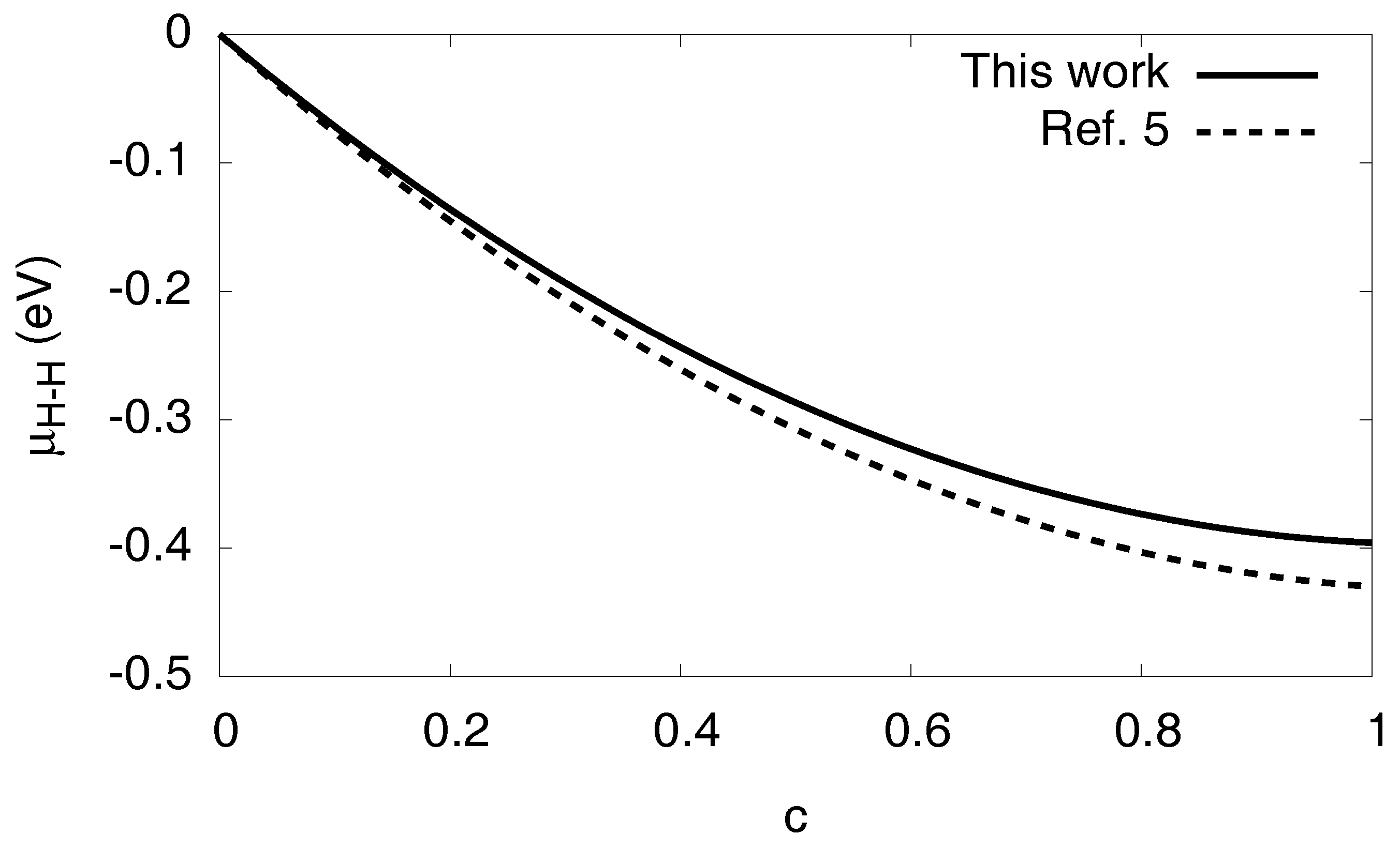
and is split into additive contributions analogous to the free energy in Equation (1). We therefore get for the chemical potential contribution by the H–H interaction . It is shown in Figure 4 for both the present fitting parameters and the ones given in Ref. [5], exhibiting only small differences between the predictions.
3.4. Configurational Entropy
The configurational free energy stems from the different possibilities to occupy the interstitial sites with hydrogen (or the hydride with vacancies), and is therefore given by
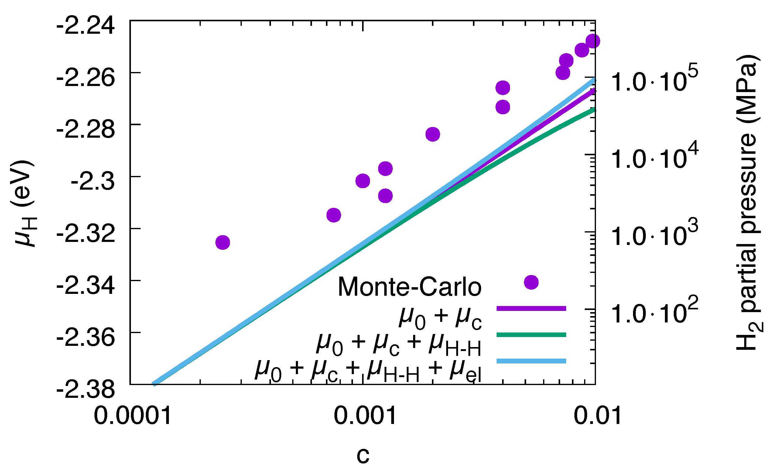
under the assumption of equal occupation probability for all octahedral sites [20]. In the low concentration regime, it gives the dominant nontrivial contribution, as elastic and interaction effects are negligible there, see Figure 5.
We note that the configurational term is the only temperature dependent one in the present description. To verify this dependence we also computed in the Monte Carlo simulations cases with different temperatures, and the results are shown in Figure 6, showing very good agreement.
3.5. Maxwell Construction
Thus far, the system is described for a single phase state only, and elastic effects are suppressed by a free volume expansion. Due to homogeneity, elastic stresses as well as interfacial contributions do not appear, and the description is therefore complete on this level.
According to the usual thermodynamic picture, a single phase state is unstable in regions where the slope of the chemical potential is negative, , and phase separation should occur there. As can be seen in Figure 6, this is the case for a wide concentration regime for low temperatures, whereas for high temperatures the hydrogen solubility limit is significantly larger.
Phase coexistence on this level is described by Maxwell’s equal area rule, which states that phase separation sets in at the intersection points of a horizontal line with the S-shaped van der Waals loop, cutting it into two equal areas above and below this Maxwell line. This is shown in Figure 2 for . From this, we get the constant chemical potential in the two-phase region, for . In equilibrium, the system therefore enters the two-phase region at the first intersection of the horizontal Maxwell line with the S-shaped single phase curve. Apparently, this happens already for very low concentrations in the ppm range. Nevertheless, on the following ascending part of the curve , the system is still metastable. We point out that, according to the principles of the two-phase construction, the dual phase hydrogen chemical potential should be constant and equal to until the phase transformation is completed. Obviously, this is not the case for the atomistic data with the fixed volume constraint.
3.6. Elastic Effects
Before entering into a detailed analysis of elastic effects, let us briefly discuss them in relation to the H–H interaction term. The latter is sometimes also introduced as long-range elastic interaction, and we want to stress that we do not double count effects here. The H–H interaction term expresses that an H atom locally deforms the lattice, and therefore makes the placement of another H atom in the vicinity energetically favorable. In a mean field context, this is expressed by the term ∼ in . If the site occupancy gets higher and the octahedral sites more and more filled, the energy for placing more H atoms into the lattice increases again, as expressed by the term. Although this consideration makes reference to elastic deformations, this is distinct from the elastic effects considered in the following. To make this point more explicit, we consider the following two situations, for simplicity both with homogeneous hydrogen distributions, i.e., spatially constant concentration c:
First, for fixed pressure , we increase the hydrogen concentration. This leads to a widening of the lattice, as discussed in the following and shown in Figure 7. However, since the system remains stress free on a mesoscopic or macroscopic level, , the elastic energy (see Equation (5)) in the continuum mechanics sense remains zero. Nevertheless, the total energy of the system is changed due to the H–H interaction, and this is expressed through , which is independent of the elastic stress state.
Second, for fixed concentration (and total number of hydrogen atoms), we change the external pressure of the system. Then, the H–H interaction term does not change, but the mesoscopic elastic energy does.
The difference between the H–H interaction term and the explicit elastic term becomes most prominent in two-phase situations. Then, the hydride has a larger equilibrium lattice constant and therefore distorts the surrounding, coherently connected matrix phase. This leads to long-ranged elastic deformations, and the range of these interactions of the order of the precipitate size, which is captured by the mesoscopic elastic energy term introduced below, but not by the H–H interaction term. For further discussion of this separation of microscopic and mesoscopic elastic contributions, we refer to [8]. There, it was shown that the elastic energy due to microscopic deformations around individual H atoms and long ranged strains resulting from the formation of mesoscopic precipitates decompose additively into microscopic and mesoscopic contributions without the appearance of a cross term.
The large deviations between the atomistic data and the continuum model clearly indicate that elastic and interfacial effects are critical and cannot be neglected. We remind that the basis for the Maxwell construction—or here equivalently the common tangent construction—is based on the assumption that the two-phase energy in a macroscopic system decomposes additively into the contributions of the two phases, which do not influence each other. This means, that they are described by free energy densities, which depend only on the local concentration. This condition, however, is violated in the presence of elastic effects. Here, e.g., a density variation in one phase also influences the other, as the global pressure in the system changes.
In the following, we discuss the modeling mainly from the continuum perspective. The technical aspects of the parameter matching between the scales are given in the appendices.
We focus first on the low-temperature regime, where the hydrogen solubility limit is low (see Figure 13), and higher temperatures will be discussed later. In the present regime, the phases are almost stoichiometric, and the chemical potential of the hydrogen in the two-phase region is modified. From a minimization of the total free energy in the two-phase region, we obtain the modified chemical potential (see Appendix A)
In contrast to the Maxwell term , the elastic and interfacial contributions, and , respectively, do depend on the concentration, and therefore the chemical potential is no longer constant in the two-phase region, as observed in the Monte Carlo simulations (see Figure 2).
3.6.1. Linear Elastic Effects
The pure nickel and the hydride exhibit a substantial lattice mismatch, and therefore, in the two-phase region, elastic stresses arise. The linear elastic free energy density per unit volume is given by
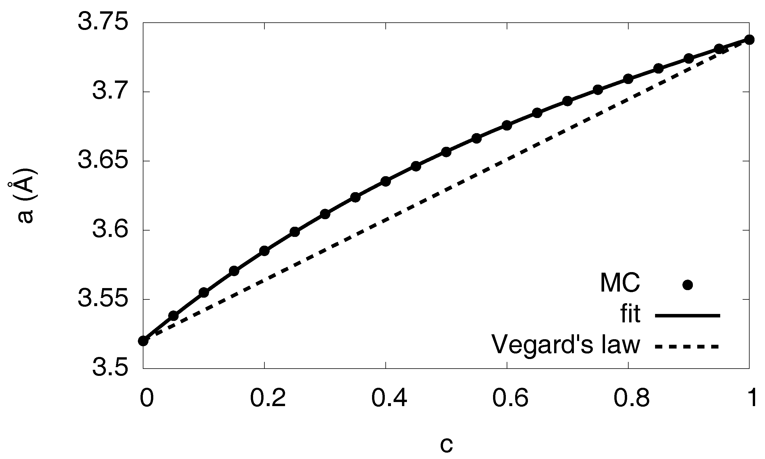
where is the strain derived from the displacements , and the eigenstrain represents the isotropic volume expansion of the hydride [21]. It is concentration dependent, and we extracted it again from simulations of homogeneous states with ; it is well described by with fitting parameters , and , going beyond a linear dependence in the spirit of Vegard’s law. The eigenstrain is directly related to the concentration dependent lattice constants with and via , since we use here the relaxed, hydrogen-free nickel as reference configuration (see Figure 7).
The elastic constants for the pure phases are listed in Table 1. We note that all values are given with respect to Ni as reference configuration; see Appendix B for a discussion of this issue. The determination of the elastic constants from the Monte Carlo simulations is described in detail in Appendix C.
To better understand the role of the elastic effects, it is instructive to inspect an analytical isotropic linear elastic model, where we assume for simplicity the elastic constants to be equal in both phases. We use a spherical sample of radius R consisting of nickel, with a hydride inclusion of radius in its center. The radial displacement component is continuous at the coherent interface and vanishes at the outer boundary due to the volume constraint. At low temperatures, the concentration is in good approximation in Ni and in the hydride. This gives (see Appendix D)
where is the number of octahedral sites per unit cell, , and and G are Lamé coefficient and shear modulus respectively. In this approximation, the elastic contribution in Equation (6) is a linear function of the concentration, and it depends quadratically on the eigenstrain difference . Since the material is relaxed for , the elastic effects therefore give only an additive constant for , which is related to the elastic hysteresis due to the internal stresses that arise upon precipitate formation. For the isotropic elastic constants we use the values for nickel and and for the solid curve in Figure 8.
The calculation can also be done using the elastic constants of the individual phases, leading to the long-dashed curve shown in the same graph (see Appendix D). A numerical finite element solution with ABAQUS for spherical precipitates in a cubic box with fixed volume, taking into account the full cubic elasticity and periodic boundary conditions, leads to the short-dashed curve shown in Figure 8. It is very close to the analytical results. Since we still observe a significant discrepancy to the Monte Carlo data, we conclude that the consideration of linear elasticity is not sufficient to explain the slope of the chemical potential in the two-phase region.
3.6.2. Nonlinear Elastic Effects
The reason for the discrepancy between the atomistic data and the continuum modeling involving linear elasticity is the appearance of large compressive stresses for higher hydrogen concentrations (at fixed volume), and therefore the linear elastic approximation breaks down. Instead, we have to take into account nonlinear elastic effects; they include nonlinearities in the stress-strain relationship, leading effectively to expressions in the elastic free energy density. Additionally, geometrical nonlinearities appear due to the volume deformation and the nonlinear strain tensor [11],
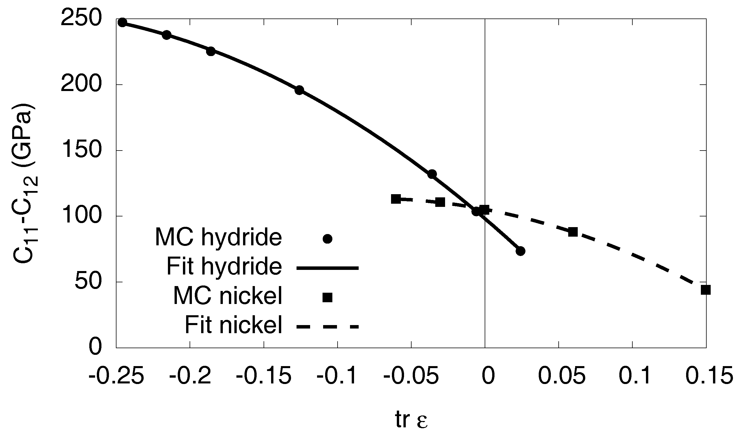
We have estimated that these effects are small in comparison to the change in the constitutive law, and therefore effectively captured them in the modified elastic constants. However, it turns out to be important to carefully use consistently the same reference configuration for the Lagrangian formulation of elasticity for both phases. We note that the chemical potential contains now also a contribution due to the strain dependence of the elastic constants. We mention in passing that we do not observe plastic deformations in the atomistic simulations. From a careful analysis of the Monte Carlo simulations we find that the nonlinear corrections depend only on the volume change and not on shear effects, thus the elastic constants depend only on the trace of the (local) strain tensor, which simplifies the expressions. We therefore write them as series expansion
for all elastic constants or combinations of them. From the atomistic simulations we find the coefficients of the nonlinearities for , and the bulk modulus K, see Table 2 and Appendix C. From them, all elastic constants can be expressed using the relation . We note that for the present geometry bulk compression is the dominant effect, and the material becomes stiffer in this regime of negative strain (compression). Including the nonlinear contributions the continuum chemical potential shows now a very satisfactory agreement with the Monte Carlo data, see the dotted line in Figure 8.
3.7. Interfacial Effects
In a final step, we take into account interfacial effects. As already visible from the agreement of the Monte Carlo data and the nonlinear elastic curve, their contribution is obviously small. In isotropic approximation, the surface energy for a spherical inclusion is given by with the surface energy . From planar interface calculations, we obtain for (100) interfaces and for (111) interfaces. From the fitting of two-phase data, we independently get an excellent agreement using for the spherical inclusion.
The magnitude of interfacial terms should be compared to bulk contributions to see their influence and to get an impression on the dimension of critical nuclei. For an order of magnitude estimate, we compare elastic bulk contributions in the approximation in Equation (6) to interfacial contributions for spherical precipitates for small concentrations in Equation (A42), where the influence of interfacial terms is largest. For the elastic and interfacial contributions are comparable for
which is the case for about 23 H atoms. This indicates that interfacial contributions are indeed small for the present scenario in comparison to the elastic bulk terms.
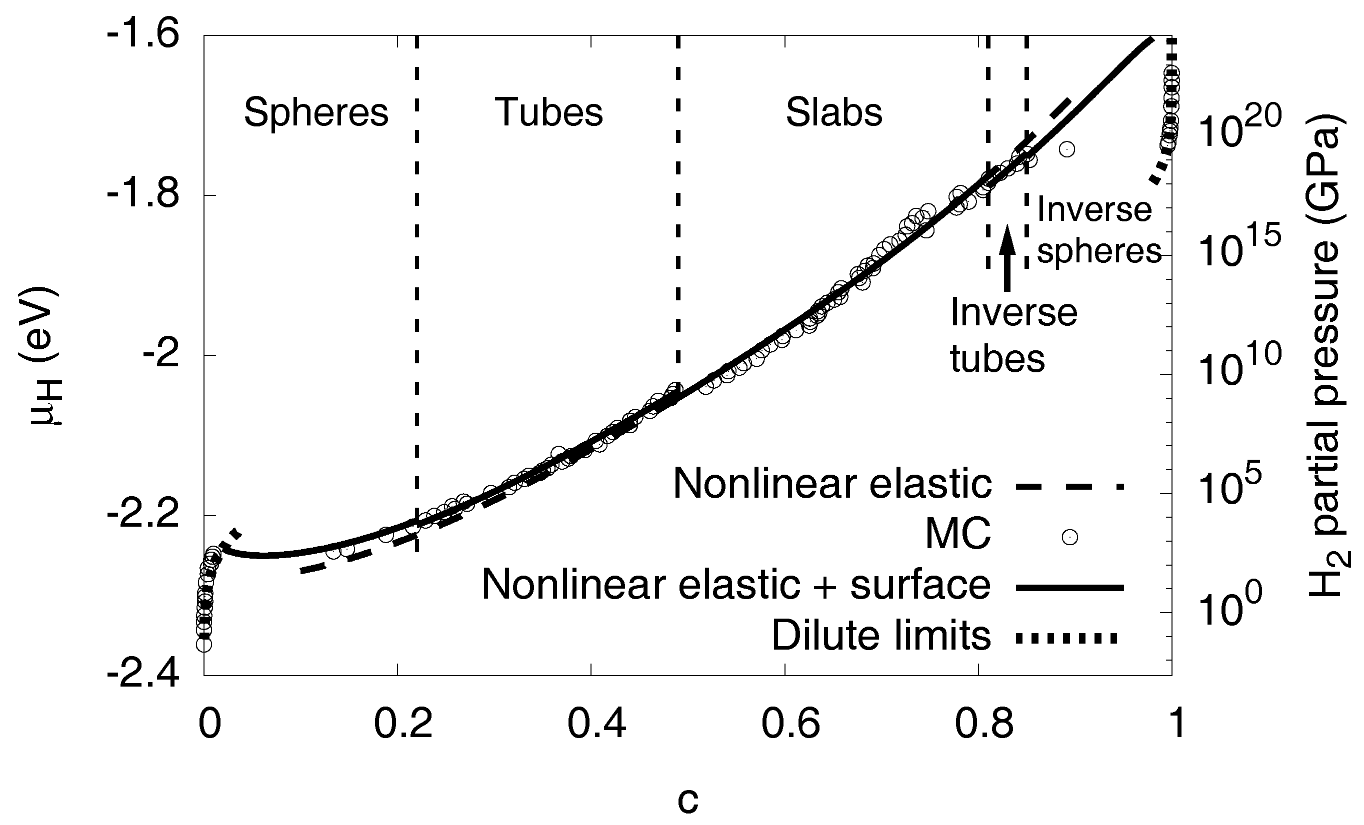
For a linear isotropic material with equal elastic constants in both phases and a purely dilatational eigenstrain, the elastic energy does not depend on the shape of the inclusion but only on its volume fraction [22]. Although the conditions for this rigorous statement are not exactly fulfilled here, we find only a small dependence of the elastic energy on the precipitate shape in the Monte Carlo data, as exemplarily shown for spherical hydride inclusions in a Nickel matrix and vice versa in Figure 9. Consequently, the shape of the precipitate is determined by the interfacial energy terms alone, see Appendix E for explicit calculations. This means, that for each given average concentration c, which is related to a precipitate size, the equilibrium shape with the minimum interfacial energy appears. For isotropic surface energy we expect spherical inclusions for , followed by tubes up to , and slabs thereafter. The situation is symmetric for with then the hydride being the matrix phase. Thus we expect nickel tubes in the range and spheres beyond this concentration. In our Monte Carlo calculations, we indeed find all these structures in the correct ordering (see Figure 1 and Figure 10), but the transition points differ slightly due to anisotropy and nonlinear elastic effects. Based on the observed structures and the calculated interfacial energy we added this contribution to the nonlinear elastic chemical potential in Figure 10. The transitions between different precipitate shapes explain the small discontinuities in the chemical potential, as computed from the Monte Carlo simulations. Apparently, with all the aforementioned effects taken together, we get an excellent agreement with the Monte Carlo data in the entire two-phase region.
Finally, we briefly comment on the role of surface stress. In isotropic approximation, the surface energy for a spherical inclusion is given by with the surface energy . The surface stress contribution is in spherical coordinates, with the scalar surface stress coefficient [23,24]. We obtain—in the same approximation as for Equation (6)—due to the additional pressure difference between the precipitate and the matrix also a contribution from the elastic bulk energy [25]
where we have neglected a small destabilizing term proportional to for (we have estimated from the atomistic data to be of the order , thus this condition is fulfilled), and also assumed , since spherical precipitates appear for small concentrations only, as discussed below. Consequently, these terms have the same radius scaling as the surface energy term ∼, and despite their partial origin from a bulk energy, they appear effectively as surface term; therefore, we treat them via a renormalized interfacial energy density .
With this, the parametrization of the continuum model is completed, and it is used in the following for predicting hydrogen partial pressures, volume relaxation effects, and for the prediction of phase diagrams.
3.8. High Concentration Limit
We can also correctly describe the limit of high hydrogen concentrations, where almost all octahedral sites are filled with H. For , the system is again in a single phase state, with a dilute distribution of vacancies, thus the steep divergency of the chemical potential is due to the configurational degrees of freedom. Nevertheless, the central difference to the dilute limit is that the material is here severely under (nonlinear) stress (as we focus on fixed volume situations, where pure Ni is stress free, hence stresses are maximized for ) , thus elastic effects play a major role here. In contrast to the phase separated region we need precise knowledge of the concentration dependence of the elastic constants, their nonlinearities and the eigenstrain. Consideration of all these effects leads to the good agreement between the Monte Carlo data and the continuum picture, as shown in Figure 10.
3.9. Conversion to Partial Pressures
To relate the chemical potentials to experimentally accessible quantities, it is useful to translate them to hydrogen (H) partial pressures. In the following, we use a subscript to discriminate between quantities related to the gaseous hydrogen molecules and the monatomic hydrogen in solid solution. From the ideal gas equation and the Maxwell relation
we obtain by integration the chemical potential of up to an additive term ,
with an arbitrary reference pressure . From the equilibrium between and dissociated hydrogen follows
This leads to
We therefore need an expression for to link the chemical potential to a hydrogen partial pressure.
In the dilute limit , the chemical potential is (see also Figure 5)
This is in agreement with experimental findings [26] for the solubility of H in Ni
expressed in terms of the quantities used here, with and (the prefactor 2 stems from the dissociation of a H molecule in two H atoms). This allows to identify an expression for the offset potential
where we have chosen . With these identifications, Equation (14) is the desired relation, which is shown in Figure 10. Apparently, the H partial pressures needed for the higher concentrations are extremely high and not reachable in experiments under normal conditions, making computer simulations particularly useful there. In addition, we note that for such high pressures the used ideal gas description of H breaks down. On the other hand, the H partial pressures needed for formation of a hydride are much lower for free volume situations, which will be discussed below (see Figure 11). We can therefore conclude that volumetric constraints, or—more generally—compressive stresses can suppress the formation of hydrides, which can be responsible for the embrittlement of the metal.
3.10. Volume Relaxation
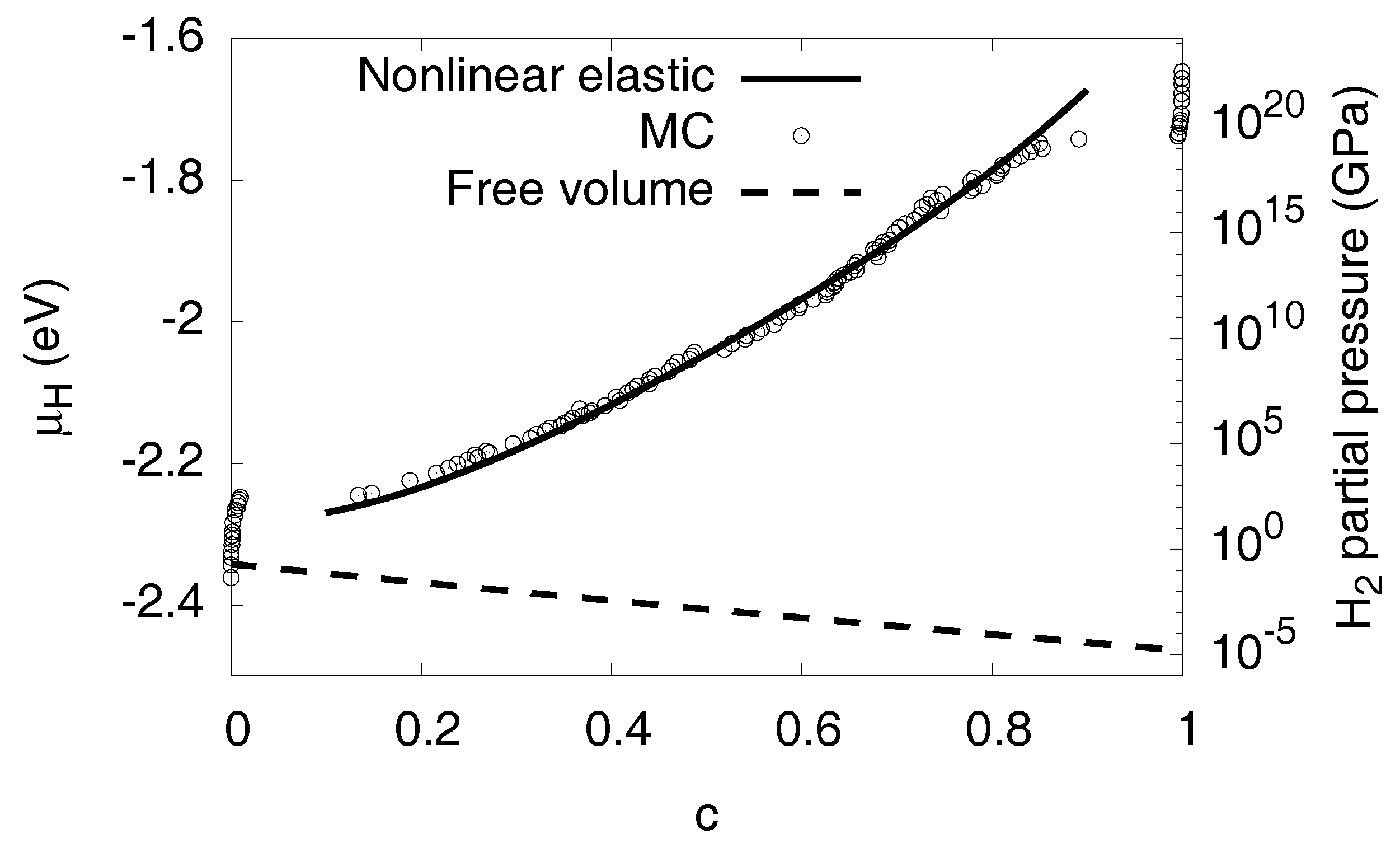
Instead of a fixed volume constraint, one may also consider a situation with free expansion, . This does not mean that elastic effects disappear, because in the two-phase region internal coherency stresses still arise. Thus, the same elastic barrier appears for the first nucleation of the precipitate, but thereafter the elastic contribution to the chemical potential decreases with concentration, see Figure 11. Since the stress effects are much lower, elastic nonlinearities are negligible here, and the curve is calculated in linear isotropic approximation. The qualitatively different behavior shows the important role of external boundary conditions. In contrast to scenarios with free expansion, the volume constraint stabilizes two-phase equilibria. This behavior can intuitively be understood as follows: When a precipitate is inserted into the matrix, coherency stresses arise, which increase the elastic energy. If the precipitate grows and finally fills the whole sample, the freely expanding material is homogeneous and therefore stress free. This implies that the elastic energy decays with the hydride volume fraction, and therefore the elastic contribution to the chemical potential appears with negative sign. Therefore, we get a hydrogen chemical potential with a negative slope in the two-phase region, which corresponds to an unstable situation. We have verified this prediction using Monte Carlo simulations for fixed and free volume at , see Figure 12.
We note that volume constraints can therefore stabilize precipitates. In a simulation, this is useful for probing situations with phase coexistence, which would otherwise not appear, as either the system is homogeneously in the dilute state or fully saturated with H for given chemical potential. This is expressed here by a negative slope of the chemical potential of H. The present physically motivated approach is therefore an alternative to bias potentials [12] to probe configurations with phase coexistence.
3.11. Phase Diagram
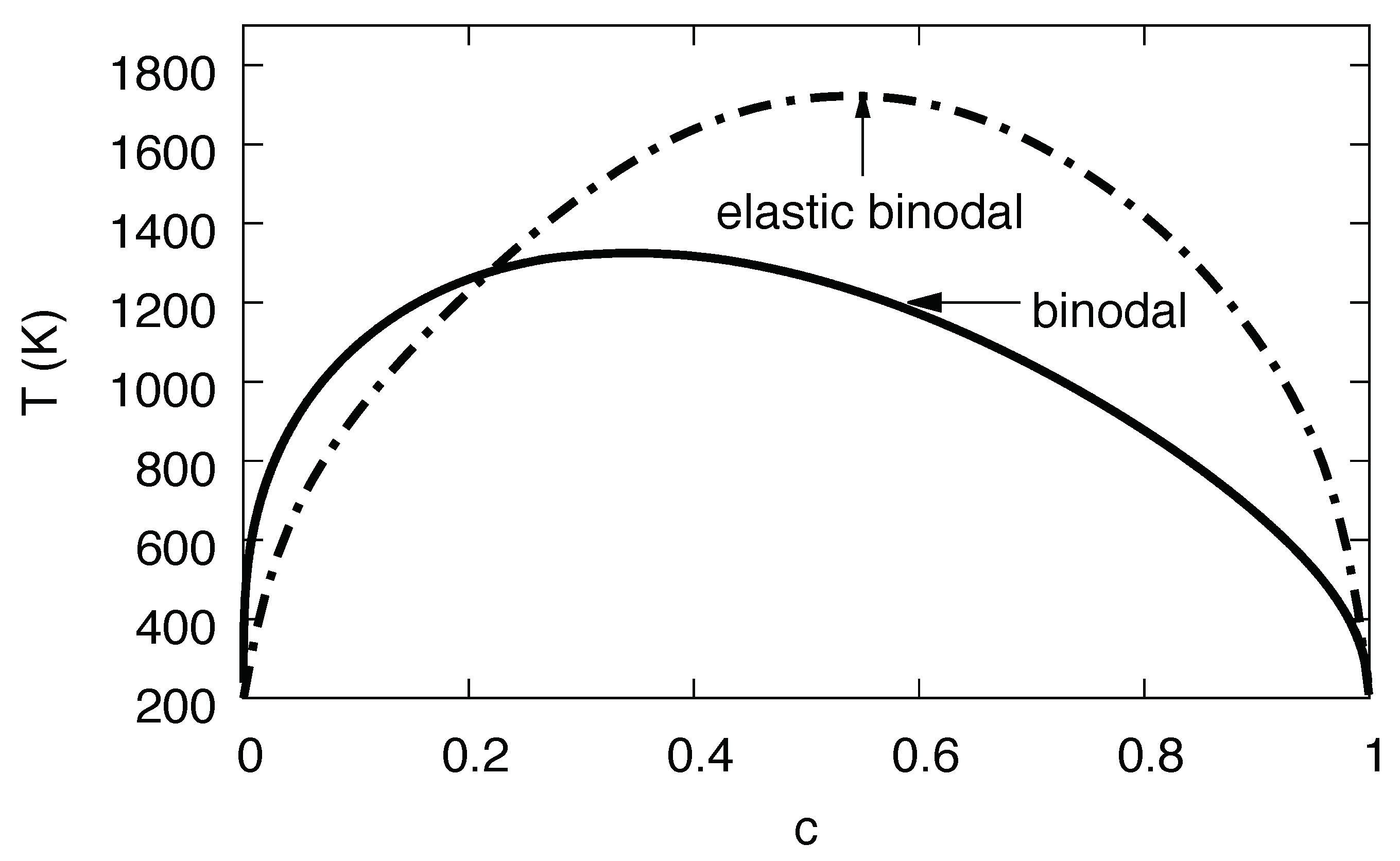
Based on the temperature dependence of , we can predict the entire bulk phase diagram without elastic effects via the Maxwell construction, see Figure 13. We note that this phase diagram is derived solely from data for the H–H interaction. To verify it also for higher temperatures, we have compared the analytical expression for the chemical potential to the single-phase data from grand-canonical Monte Carlo simulations with free volume relaxation, where elastic and interfacial effects do not appear, and find an excellent agreement (see Figure 6). We note that the purpose of the present work is to match a continuum description of Ni-H to Monte Carlo simulations based on an empirical interatomic potential. The agreement between the two theoretical approaches is excellent. Compared to experimental values, however, the description is less suitable for high temperatures, and therefore it is not accurate in this regime. The reason is—apart from potential limitations of the interatomic potential—the use of the (lattice) Monte Carlo molecular statics description, which neglects in particular phonon excitations.
An application that we can readily extract from the above results is the phase diagram taking into account elastic effects. In particular, we consider the situation of fixed volume and determine the two-phase region by minimization of the total free energy. For the sake of simplicity, we assume a slab geometry with the phase normal in direction (see Figure 14), which is the most relevant pattern in the medium concentration regime, as discussed above in Figure 10. In contrast to other geometries, homogeneity implies the constancy of concentrations in each phase. We neglect the elastic nonlinearities, which allows for a straightforward solution of the underlying one-dimensional elastic problem. As the elastic constants were determined mainly for and , we assume additionally that they interpolate linearly for arbitrary concentrations . This is mainly relevant for higher temperatures, where the appearing phases have larger solubilities for hydrogen or vacancies, thus they appear with intermediate concentrations. As will be discussed below, it turns out that the concentration dependence of the elastic constants is not important, and therefore this approximation is legitimate.
We inspect the case of a constant total volume which is stress free for pure nickel, i.e., the lattice constant for a homogeneous system is . Consequently, for the two-phase system with cubic symmetry, the only non-vanishing displacement component is , which is a linear function of x in each phase, (the phases are enumerated by i). Hence, the only nontrivial strain component is ; stresses follow from Hooke’s law with cubic symmetry,
Because the concentration is homogeneous in each phase for this effectively one-dimensional situation, the linear bulk elastic equations are automatically fulfilled by the above ansatz. The coefficients are determined by the boundary and matching conditions, , and . The elastic energy density is in each phase
From that, we can calculate the elastic energy per unit area,
The total free energy is then . Additionally, the concentrations and in the two phases are related to the (fixed) average concentration c via the lever rule,
We can therefore investigate as function of for given values of , and the phase fractions are determined by the lever rule. The concentration domain can be restricted to , and the free energy is minimized with respect to and in equilibrium. Whenever the minimum is located inside this domain, the system is in a two-phase state, whereas the minimum is located on the border or for a single phase state. By performing this minimization in the entire plane one obtains the elastic phase diagram.
Already at this level we see the tremendous influence of the elastic effects in Figure 13, with an enlargement of the two-phase region towards higher temperatures and the hydrogen rich side. This unusual behavior—one would intuitively expect the suppression of phase separation since coherency stresses are energetically unfavorable—is due to the fact that the eigenstrain is a concave function of the concentration, (see Figure 7), thus volumetric deviations from Vegard’s law play the dominant role here.
To investigate this peculiarity in more detail, we look at the elastic energy depending on the phase concentrations. We start with a situation which differs from the true Ni-H problem. Instead, we assume a linear dependence of the eigenstrain on concentration (see Figure 7) (Vegard’s law). Here, we find that single-phase states have the lowest elastic energy in a wide region of the phase diagram and are therefore energetically favorable. Thus, phase separation is suppressed by elastic effects in this fictitious situation, leading to an increased H solubility limit, and this is shown in Figure 15. In contrast, for the true concentration dependence of the lattice constant on the H concentration in Figure 7, we obtain a reduced solubility limit of hydrogen in the nickel matrix. As mentioned above, this is a counterintuitive result, as the appearance of phase separation should usually increase the elastic energy and therefore make this state thermodynamically unfavorable, in contrast to our observation. Here, the situation is opposite: Single-phase states are more expensive from point of view of elastic energy, and the hydrogen solubility limit is therefore reduced. The explanation is that the single-phase case has a higher average eigenstrain, and therefore the mechanical volume work is higher than for the phase separated case for the anticipated fixed volume ensemble.
As a result, we find that the dependence has a tremendous influence on the phase diagram. This effect is much more pronounced that the concentration dependence of the elastic constant. If we assume, instead of the linear interpolation between the values for Ni and Ni-H, just concentration independent constants using the values of Ni, we find only a small shift of the binodal (see Figure 15). We can therefore conclude that the concentration dependence of the lattice constant is the most relevant quantity for the influence of elastic effects on hydrogen solubility limits.
4. Discussion and Conclusions
Understanding the thermodynamics of phase separation across the scales is a key for deriving macroscopic material properties from fundamental microscopic descriptions. Often, such a transfer is not straightforward, but, with careful descriptions, it is possible to obtain not only macroscopic parameters but also describe energy functionals in agreement with the underlying behavior on atomic scales. We demonstrated such an approach for the Ni-H system with a special focus not only on classical thermodynamics but also strong mechanical and interfacial effects.
In detail, we have seamlessly matched the results of hybrid molecular static and Monte-Carlo simulations in a binary system with full consideration of elastic effects to a continuum description for large scale simulations. The accurate identification of configurational, interaction, nonlinear elastic and surface effects allows for a thorough understanding, which will be equally useful and applicable to other mechanisms or material systems. Presently, the description is most useful for the low temperature regime below the Debye temperature. The consideration of vibrational degrees of freedom and defect formation, as well as the consideration of more complex phase diagrams will be the subject of future investigations. It should be pointed out that the accuracy of the predictions is limited by the atomic scale description, to which the continuum energy functional is tailored. The inclusion of the effects mentioned before will presumably require the consideration of additional energy terms and variables such as defect concentration.
The determination of phase diagrams demonstrates the opportunities arising from the transfer of atomistic data to the mesoscale: The quantitative determination of the free energy allows for example to construct the entire phase diagram in Figure 13 computationally much more efficiently than using atomistic simulations which require large system sizes and long relaxation times, especially in the room temperature regime. Moreover, the description serves as an accurate basis for mesoscale simulation methods such as phase field [27].
Acknowledgments
This work was supported by the DFG Collaborative Research Center 761 Steel ab initio. The authors gratefully acknowledge the computing time on the supercomputer JURECA at Forschungszentrum Jülich.
Author Contributions
All authors contributed equally to this work.
Conflicts of Interest
The authors declare no conflict of interest.
Abbreviations
The following abbreviation is used in this manuscript:
| MC | Monte Carlo |
Appendix A. Thermodynamic Framework
To understand the influence of elastic effects on the phase diagram and the chemical potential, we start with considering the free energy of the system. We use the following notations: is the total number of nickel atoms, is the number of Ni atoms in the dilute phase, is the number of Ni atoms in the hydride, and is the number of nickel atoms per unit cell (4 for fcc). Similarly, is the total number of hydrogen atoms, with of them being in the dilute phase and in the hydride. In the fully saturated hydride, we have hydrogen atoms per unit cell (here, ), which corresponds to the normalization . Thus, we define the hydrogen concentration in the dilute phase , and in the hydride, . The average concentration is .
The free energy of the system is
Here, is the free energy density (per host atom) of the dilute phase, and is the same for the hydride. The elastic energy depends on the volume fractions and the concentrations in each phase. Here, we already suppressed the degree of freedom of the shape of the hydride inclusion and assume that the free energy is already minimized with respect to it. Notice that we consider here only situations with fixed global strain (i.e., fixed volume), therefore the free energy is the appropriate thermodynamic functional.
As a further approximation of the elastic energy for low temperatures, we take into account that the dilute phase is almost free of hydrogen (), whereas the hydride is almost fully saturated (. This implies . Therefore, we obtain the simplification with the intensive elastic energy density .
For the determination of the two-phase equilibrium, we proceed in the usual way: The free energy has to be minimized with respect to the phase fractions and the partitioning. Therefore, we get
where we defined the chemical potentials
The equality of grand potentials becomes
Notice that the elastic terms do not appear in the common tangent construction in the framework of the above approximations, since the concentration is assumed to be fixed in this approximation, which holds here for low temperatures.
Next, we calculate the chemical potential of the hydrogen in the two-phase region. It is given by
since the last two terms vanish by the equilibrium conditions in Equations (A2) and (A4). Here, we obtain
which corresponds to Equation (4) in the main text. Interfacial effects can be considered in a similar way.
Appendix B. Reference State
For the elastic problem, we describe the material in the Lagrangian reference frame of the stress-free nickel. The eigenstrain of the hydride is therefore ; notice that also for the hydride the (eigen-)strain is defined relative to the lattice constant of the relaxed Ni. To make this point more transparent, we denote all quantities with Ni-H as reference state by a tilde, e.g., a dilatational strain by , thus apart from an additive eigenstrain contribution . Since stresses are defined as force per area in the reference configuration, we have the transformation rule . From Hooke’s law, and , we therefore conclude . This means that that the elastic constants of the hydride relative to nickel as reference state appear by a factor higher than their nominal values for Ni-H reference configuration.
Appendix C. Elastic Constants
Here, we briefly explain the extraction of the elastic constants from the Monte Carlo simulations. Notice that in the absence of vibrational contributions the elastic constants are temperature independent and are therefore calculated at . In all cases, the relaxed equilibrium configuration of pure Ni is taken as reference state, see Appendix B.
Appendix C.1. Bulk Modulus
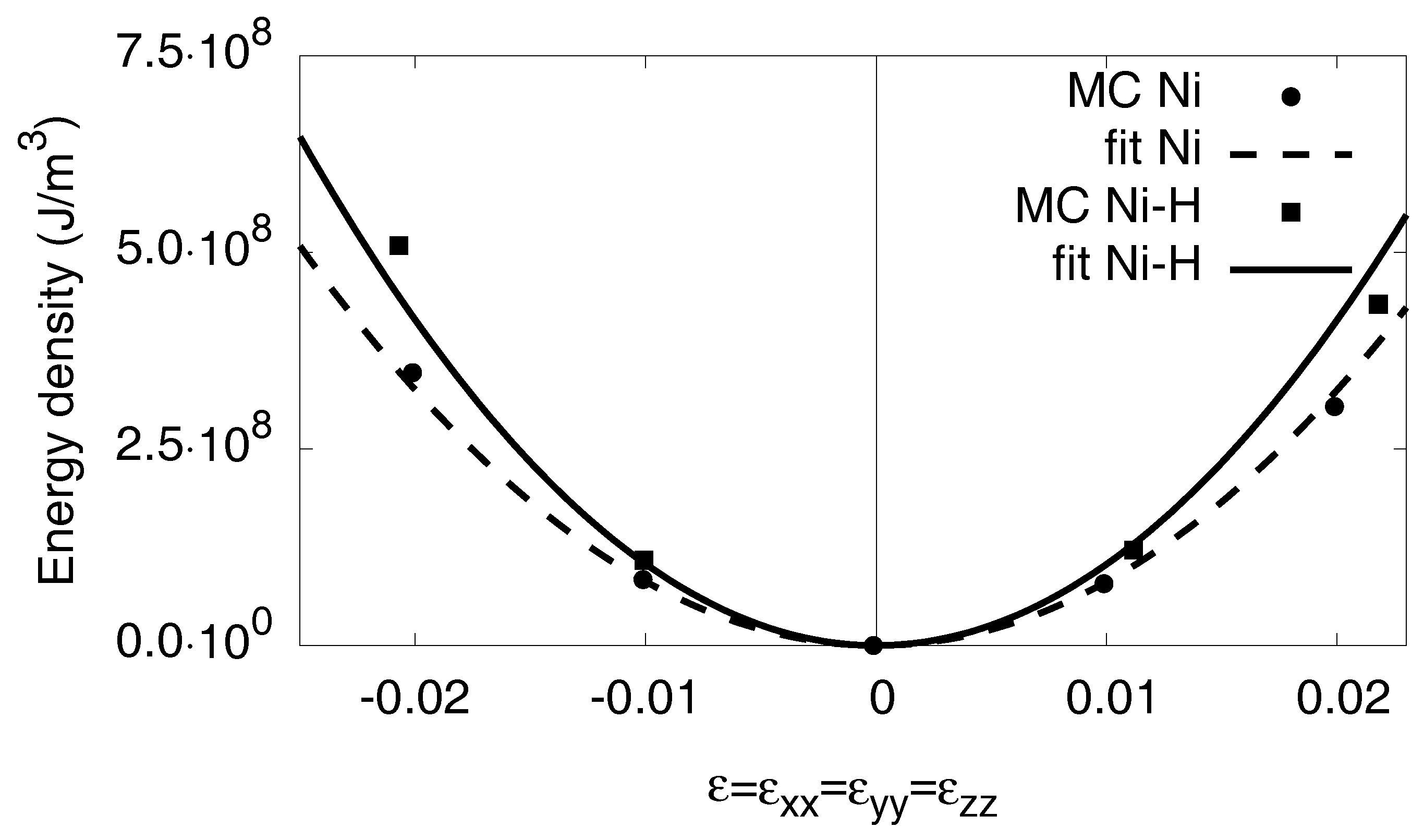
To get the bulk modulus K for the phases, we strain the system isotropically with . The resulting energies are represented in Figure A1. In linear elasticity, the energy increases quadratically with the strain,
and we determine the bulk modulus K from the curvature of the measured energy–volume curves. Hence, we get for pure Nickel and for the fully saturated hydride .
Figure A1.
Energy density as function of the external hydrostatic strain . With the relation in Equation (A7), we get the bulk modulus K in quadratic approximation. The atomistic data are taken from simulations at . For high strains deviations from the linear elastic response can be seen.
Figure A1.
Energy density as function of the external hydrostatic strain . With the relation in Equation (A7), we get the bulk modulus K in quadratic approximation. The atomistic data are taken from simulations at . For high strains deviations from the linear elastic response can be seen.
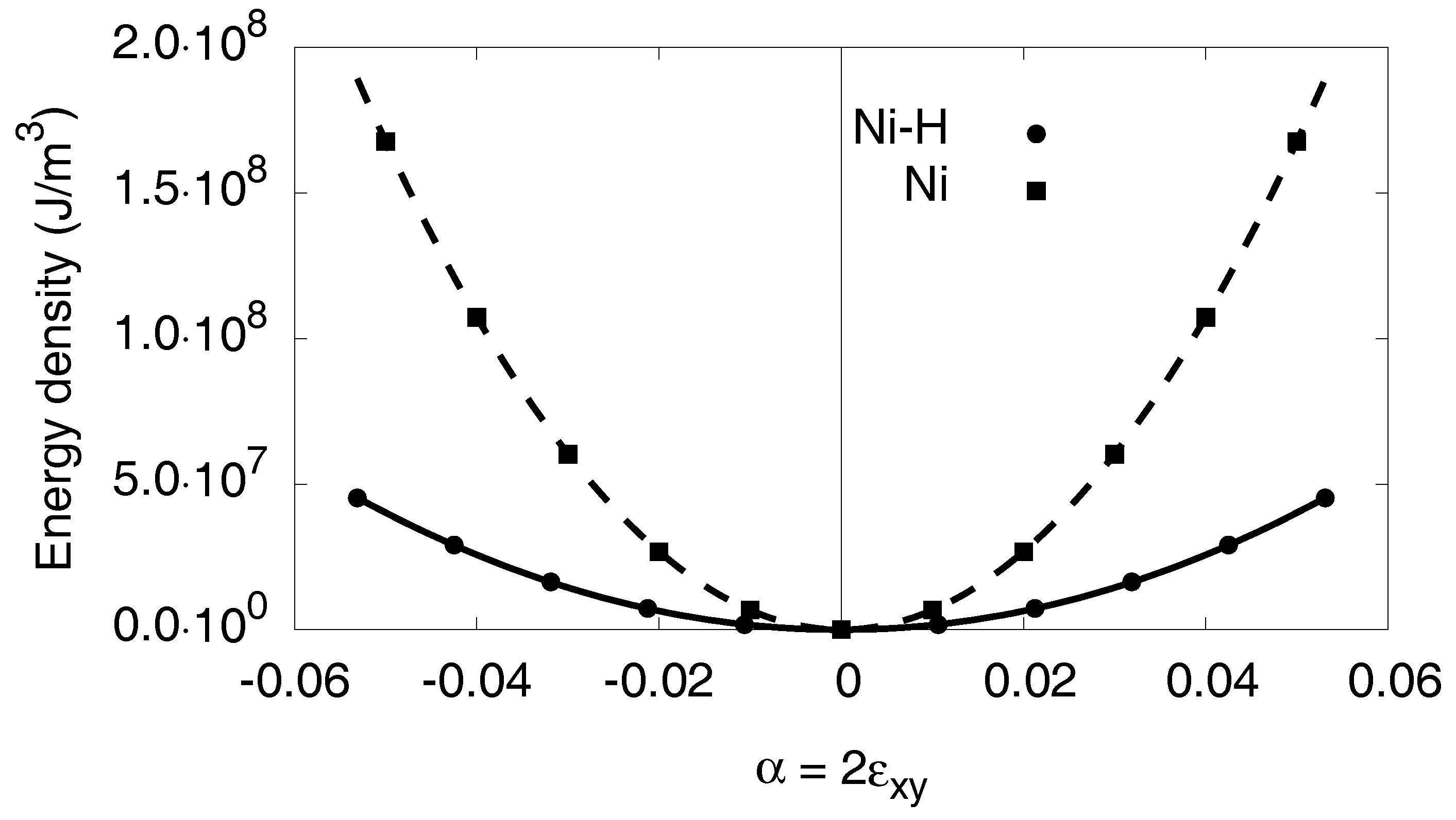
Appendix C.2. Monoclinic Distortion
The monoclinic distortion describes shear effects to get the elastic constant both for Ni and the hydride. One gets the translational movement of an atom from the original location to the new position ,
with a deformation parameter . With the displacement and the linear strain tensor , we obtain
whereas all other strains are zero and the quadratic term in can be neglected in a linear approximation. Thus, the elastic energy is
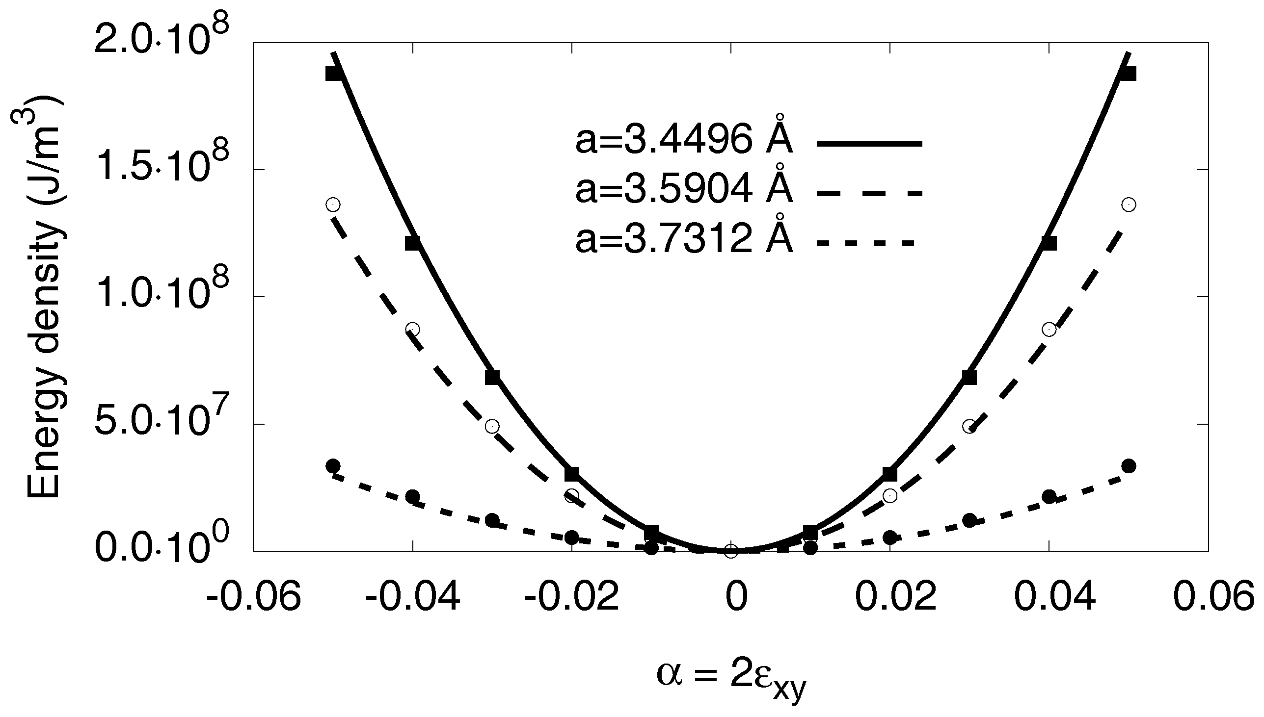
Figure A2 shows the energy density of both phases depending on the strain for the monoclinic distortion, and the elastic constant is obtained from the curvature at the origin. We obtain a value of for Nickel and for the hydride. Notice that for pure shear the quadratic energy–deformation dependence holds up to several percent of strain.
Figure A2.
The results for the monoclinic distortion are shown. The atomistic data is fitted via a quadratic ansatz.
Figure A2.
The results for the monoclinic distortion are shown. The atomistic data is fitted via a quadratic ansatz.
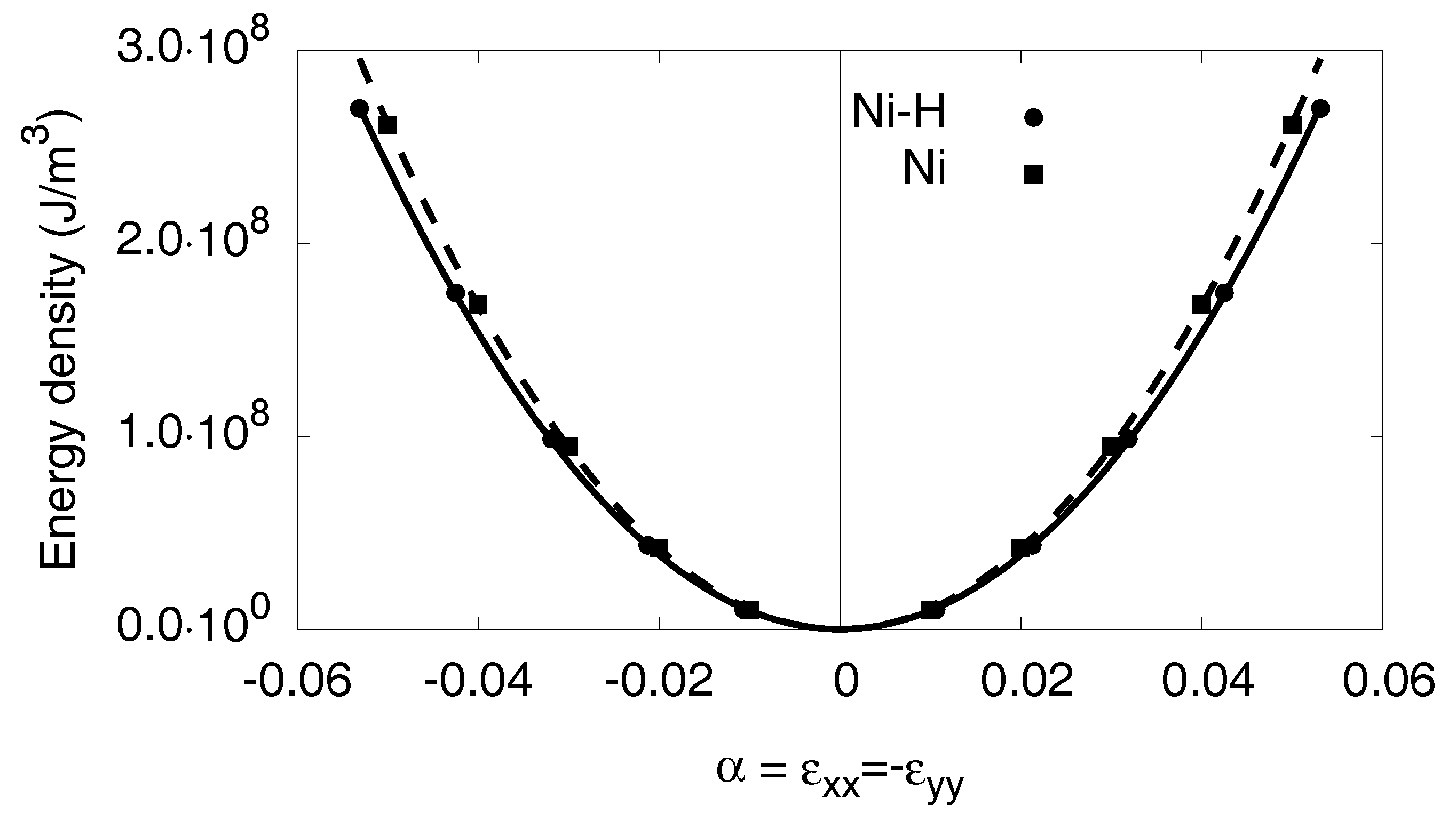
Appendix C.3. Orthorhombic Distortion
The orthorhombic distortion delivers the result for the term for both phases. It is described by
hence
where can be neglected again with the same argument as above. Consequently, the elastic energy is
The elastic constants and are
From the quadratic fit in Figure A3, we get for nickel , , and for the hydride , .
Figure A3.
The results for the orthorhombic distortion are shown. The atomistic data are fitted via a quadratic ansatz.
Figure A3.
The results for the orthorhombic distortion are shown. The atomistic data are fitted via a quadratic ansatz.
Appendix C.4. Nonlinear Elastic Coefficients
To demonstrate the extraction of the elastic nonlinearities, we inspect the mechanical response of pure Ni under bulk compression or expansion, as shown in Figure A4.
For larger strains, we see deviations from the linear response, i.e., a quadratic energy–strain relationship. For tensile stresses the material appears effectively softer, whereas it is stiffer under compression. In the strain regime shown in the plot, the elastic response is well described by
in the spirit of Equation (8). The coefficients are given in Table 2.
For pure shear during a monoclinic transformation, the energy is well described by a quadratic strain dependence, as shown before in Figure A2, and the same holds for the volume preserving orthorhombic transformation (see Figure A3). This demonstrates that the nonlinearities depend only on the trace of the strain tensor. We have performed monoclinic and orthorhombic transformations at different lattice units (i.e., bulk compression or expansion), to extract the coefficients in the spirit of Equation (8). This is exemplarily shown in Figure A5 for the monoclinic deformation of pure Ni. This allows to extract the elastic constants, here e.g., as function of the trace of the strain tensor. This dependence is shown in Figure A6. The resulting data for both phases are then described by Equation (8) with the coefficients in Table 2. The corresponding plot for the orthorhombic deformation is shown in Figure A7.
Figure A4.
The free energy density as a function of the external strain for the pure Nickel. The quadratic ansatz is only true for small strains, whereas for higher strain we have to use a nonlinear function to fit the Monte Carlo data.
Figure A4.
The free energy density as a function of the external strain for the pure Nickel. The quadratic ansatz is only true for small strains, whereas for higher strain we have to use a nonlinear function to fit the Monte Carlo data.
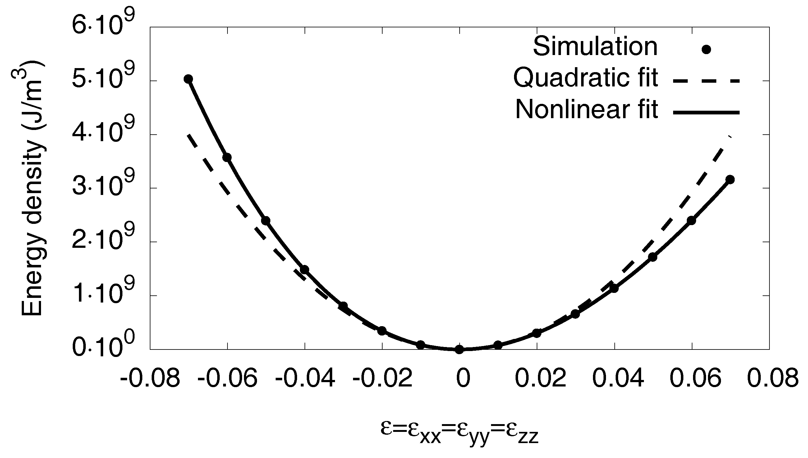
Figure A5.
Monoclinic deformation of pure nickel for different bulk lattice constants. The fits (curves) are parabolic, and the data (points) are well described without further nonlinear corrections, in agreement with the statement that corrections depend only on . The latter is contained in the lattice constant dependence of the curvatures, leading to strain-dependent elastic constants . The energy of the bulk compression is subtracted in the plots.

Figure A6.
The elastic constant as function of the trace of the strain for Nickel and the hydride is shown. For , we obtain the values: and .
Figure A6.
The elastic constant as function of the trace of the strain for Nickel and the hydride is shown. For , we obtain the values: and .
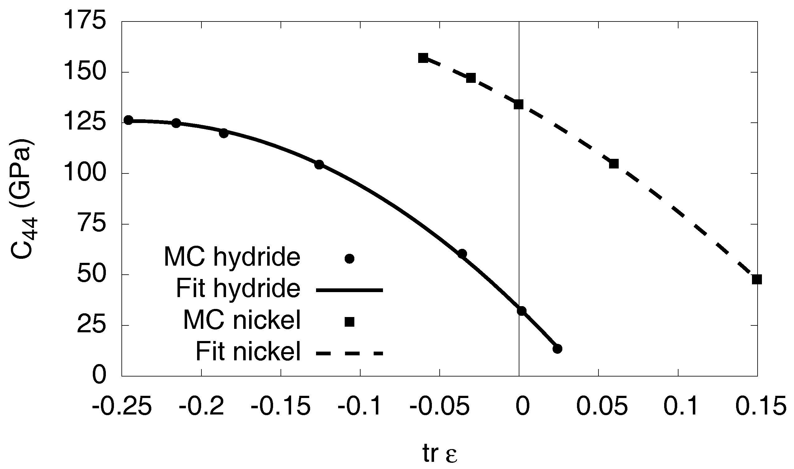
Figure A7.
The difference depending on the trace of strain for Nickel and the hydride is shown.
Appendix D. The Isotropic Model
We assume that the material is isotropic, and that a spherical nucleus of the hydride with radius forms within the dilute matrix. To simplify the geometry, we assume that the system is also spherical with radius R, thus the entire problem is rotational invariant. Hence, the displacement field depends only on the radius coordinate and has only a radial component. We note that we treat here only the linear elastic case, where corrections due to higher order terms in the strain as introduced in Equation (8) are not considered. Nevertheless, we note that the nonlinear case can also be treated in a similar way. However, for going beyond the one-dimensional case for an inclusion inside a cubic cell, we use finite element simulations instead.
In the outer dilute phase, the displacement is given by
with constants and . This ansatz satisfies the linear elastic bulk equations. In the hydride (inner phase), we use similarly
The strains are given in spherical coordinates by
and all non-diagonal terms vanish. The stresses in the dilute phase are
and in the hydride
with the eigenstrain .
At the interface coherency and stress balance demands
At the outer boundary, the fixed volume condition implies
These are altogether three conditions to determine the constants and . The elastic energy densities (per unit volume) are
and
The total free energy is
which is a lengthy expression. Using the conversions
with the lattice unit , we can calculate the elastic contribution to the chemical potential
In the general case, it becomes
In particular for equal elastic constants (, )
Appendix E. Interfacial Effects
The shape of the precipitate forming in the two-phase region is mainly determined by interfacial energy. For isotropic surface energy, a spherical inclusion minimizes the interfacial energy for small radii , with L being the edge length of the enclosing box with periodic boundary conditions. However, for , the formation of other interface contours is energetically favorable, since we use periodic boundary conditions in the atomistic and FEM simulations.
To find the different ranges and the limiting concentrations at which the forms change, we have to compute the minimum surface energy. The surface energy is defined as
where S defines the size of the interfaces and the surface energy coefficient.
First, we look for the spherical inclusion of the hydride with the radius . In this case, the surface energy is
The concentration (volume fraction) is given as
so the surface energy is
The surface energy for a hydride tube with radius r and length L is
with the respective concentration
we obtain
In the case of slabs, the surface energy is independent of the concentration c:
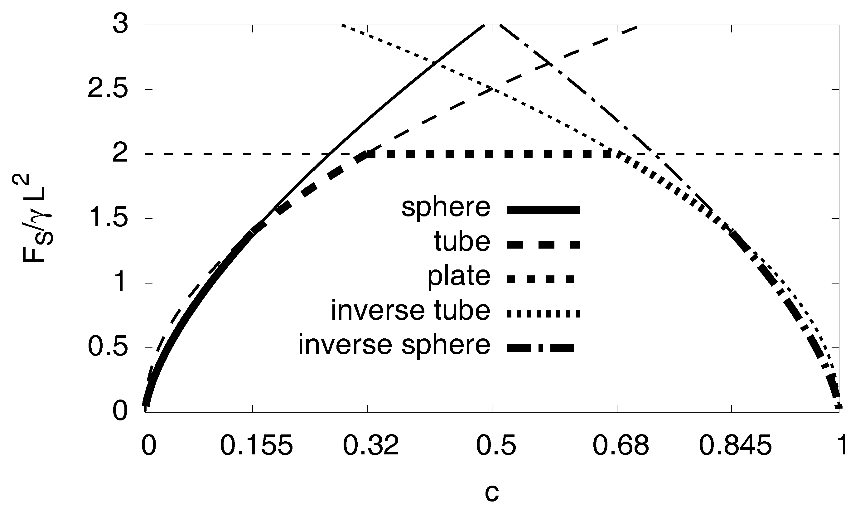
The cases with are analogous, with the role of the matrix and the hydride being exchanged. Figure A8 shows the surface energy depending on the concentration for the respective case. Up to , it should be a spherical inclusion of the hydride in the nickel matrix. For , the inclusion of the hydride should be a tube followed by plates up to . The analytical results predict a symmetric behavior for concentrations , so for concentrations there should be a tube and for we expect a nickel sphere.
Figure A8.
Surface energy depending on the concentration for different geometric cases. The thick line segments indicate the lowest energy configurations.
Figure A8.
Surface energy depending on the concentration for different geometric cases. The thick line segments indicate the lowest energy configurations.

With the calculated surface energy , we compute now the chemical potential with . Then, we have to rewrite the surface energy in an expression which depends on the number of hydrogen atoms . For the first case, the hydride sphere inclusion, the radius can be expressed as
so
The chemical potential then becomes
and finally with
Similarly, for tubes, we get
for slabs
for inverse tubes
and for inverse spheres
References
- Williams, R.O. The calculation of coherent phase equilibria. Calphad 1984, 8, 1–14. [Google Scholar] [CrossRef]
- Cahn, J.W.; Larché, F. A simple model for coherent equilibrium. Acta Metall. 1984, 32, 1915–1923. [Google Scholar] [CrossRef]
- Johnson, W.C.; Vorhees, P.W. Phase equilibrium in two-phase coherent solids. Metall. Trans. A 1987, 18, 1213–1228. [Google Scholar] [CrossRef]
- Von Pezold, J.; Lymperakis, L.; Neugebauer, J. Hydrogen-enhanced local plasticity at dilute bulk H concentrations: The role of H–H interactions and the formation of local hydrides. Acta Mater. 2011, 59, 2969–2980. [Google Scholar] [CrossRef]
- Haftbaradaran, H.; Song, J.; Curtin, W.A.; Gao, H. Continuum and atomistic models of strongly coupled diffusion, stress, and solute concentration. J. Power Sour. 2011, 196, 361–370. [Google Scholar] [CrossRef]
- Hüter, C.; Fu, S.; Finsterbusch, M.; Figgemeier, E.; Wells, L.; Spatschek, R. Electrode-Electrolyte Interface Stability in Solid State Electrolyte Systems: Influence of Coating Thickness under Varying Residual Stresses. AIMS Mater. Sci. 2016, 4, 867. [Google Scholar] [CrossRef]
- Markus, I.M.; Prill, M.; Dang, S.; Markus, T.; Spatschek, R.; Singheiser, L. High temperature investigation of electrochemical lithium insertion into Li4Ti5O12. Phys. Chem. Chem. Phys. 2016, 18, 31640. [Google Scholar] [CrossRef] [PubMed]
- Spatschek, R.; Gobbi, G.; Hüter, C.; Chakrabarty, A.; Aydin, U.; Brinckmann, S.; Neugebauer, J. Scale bridging description of coherent phase equilibria in the presence of surfaces and interfaces. Phys. Rev. B 2016, 94, 134106. [Google Scholar] [CrossRef]
- Shizuku, Y.; Yamamoto, S.; Fukai, Y. Phase diagram of the Ni-H system at high hydrogen pressures. J. Alloys Comp. 2002, 336, 159. [Google Scholar] [CrossRef]
- Fukai, Y.; Yamatomo, S.; Harada, S.; Kanazawa, M. The phase diagram of the Ni-H system revisited. J. Alloys Comp. 2004, 372, L4–L5. [Google Scholar] [CrossRef]
- Hüter, C.; Friák, M.; Weikamp, W.; Neugebauer, J.; Goldenfeld, N.; Svendsen, B.; Spatschek, R. Nonlinear elastic effects in phase field crystal and amplitude equations: Comparison to ab initio simulations of bcc metals and graphene. Phys. Rev. B 2016, 93, 214105. [Google Scholar] [CrossRef]
- Sadigh, B.; Erhart, P. Calculation of excess free energies of precipitates via direct thermodynamic integration across phase boundaries. Phys. Rev. B 2012, 86, 134204. [Google Scholar] [CrossRef]
- Laks, D.B.; Ferreira, L.G.; Froyen, S.; Zunger, A. Efficient cluster expansion for substitutional systems. Phys. Rev. B 1992, 46, 12587. [Google Scholar] [CrossRef]
- Kurta, R.P.; Bugaev, V.N.; Ortiz, A.D. Long-Wavelength Elastic Interactions in Complex Crystals. Phys. Rev. Lett. 2010, 104, 085502. [Google Scholar] [CrossRef] [PubMed]
- Metropolis, N.; Rosenbluth, A.W.; Rosenbluth, M.N.; Teller, A.H. Equation of State Calculations by Fast Computing Machines. J. Chem. Phys 1953, 21, 1087–1092. [Google Scholar] [CrossRef]
- Plimpton, S.J. Fast Parallel Algorithms for Short-Range Molecular Dynamics. J. Comp. Phys. 1995, 117, 1–19. [Google Scholar] [CrossRef]
- LAMMPS Molecular Dynamics Simulator. Available online: http://lammps.sandia.gov (accessed on 17 April 2018).
- Angelo, J.E.; Moody, N.R.; Baskes, M.I. Trapping of hydrogen to lattice-defects in nickel. Model. Simul. Mater. Sci. Engr. 1995, 3, 289. [Google Scholar] [CrossRef]
- Baskes, M.I.; Sha, X.W.; Angelo, J.E.; Moody, N.R. Trapping of hydrogen to lattice defects in nickel. Model. Simul. Mater. Sci. Eng. 1997, 5, 651–652. [Google Scholar] [CrossRef]
- Haasen, P. Physical Metallurgy; Cambridge University Press: Cambridge, UK, 2003. [Google Scholar]
- Landau, L.D.; Lifshitz, E.M. Theory of Elasticity; Pergamon Press: Oxford, UK, 1987. [Google Scholar]
- Mura, T. Micromechanics of Defects in Solids; Springer: Berlin/Heidelberg, Germany, 1987. [Google Scholar]
- Marchenko, V.I. Theory of the equilibrium shape of crystals. Zh. Eksp. Teor. Fiz. (USSR) 1981, 81, 1141. [Google Scholar]
- Fischer, F.D.; Waitz, T.; Vollath, D.; Simha, N.K. On the role of surface energy and surface stress in phase-transforming nanoparticles. Progress Mater. Sci. 2008, 53, 481–527. [Google Scholar] [CrossRef]
- Cahn, J.W.; Larché, F. Surface Stress and Chemical Equilibrium of Small Crystals. II. Solid. Particles Embedded in a Solid Matrix. Acta Metall. 1982, 30, 51–56. [Google Scholar] [CrossRef]
- Armbruster, M.H. The Solubility of Hydrogen at Low Pressure in Iron, Nickel and Certain Steels at 400 to 600∘. J. Am. Chem. Soc. 1943, 65, 1043–1054. [Google Scholar] [CrossRef]
- Brener, E.A.; Marchenko, V.I.; Spatschek, R. Influence of strain on the kinetics of phase transitions in solids. Phys. Rev. E 2007, 75, 041604. [Google Scholar] [CrossRef] [PubMed]
Figure 1.
Selected atomistic simulation results for different hydrogen concentrations with fixed volume at . The Ni matrix is not shown, and the hydrogen atoms are visualized by the dots. The equilibrium shape of the precipitates in a periodic system depends on the H concentrations. First, hydride spheres appear at low concentrations, here for (a); followed by a hydride tube (b) with . For higher saturations (here ), slabs are observed (c). Beyond , the situation is inverted and Ni precipitates form inside the hydride matrix. Snapshot (d) shows a Ni tube for . The last possible shape—a Ni sphere inside a hydride matrix—is not shown.
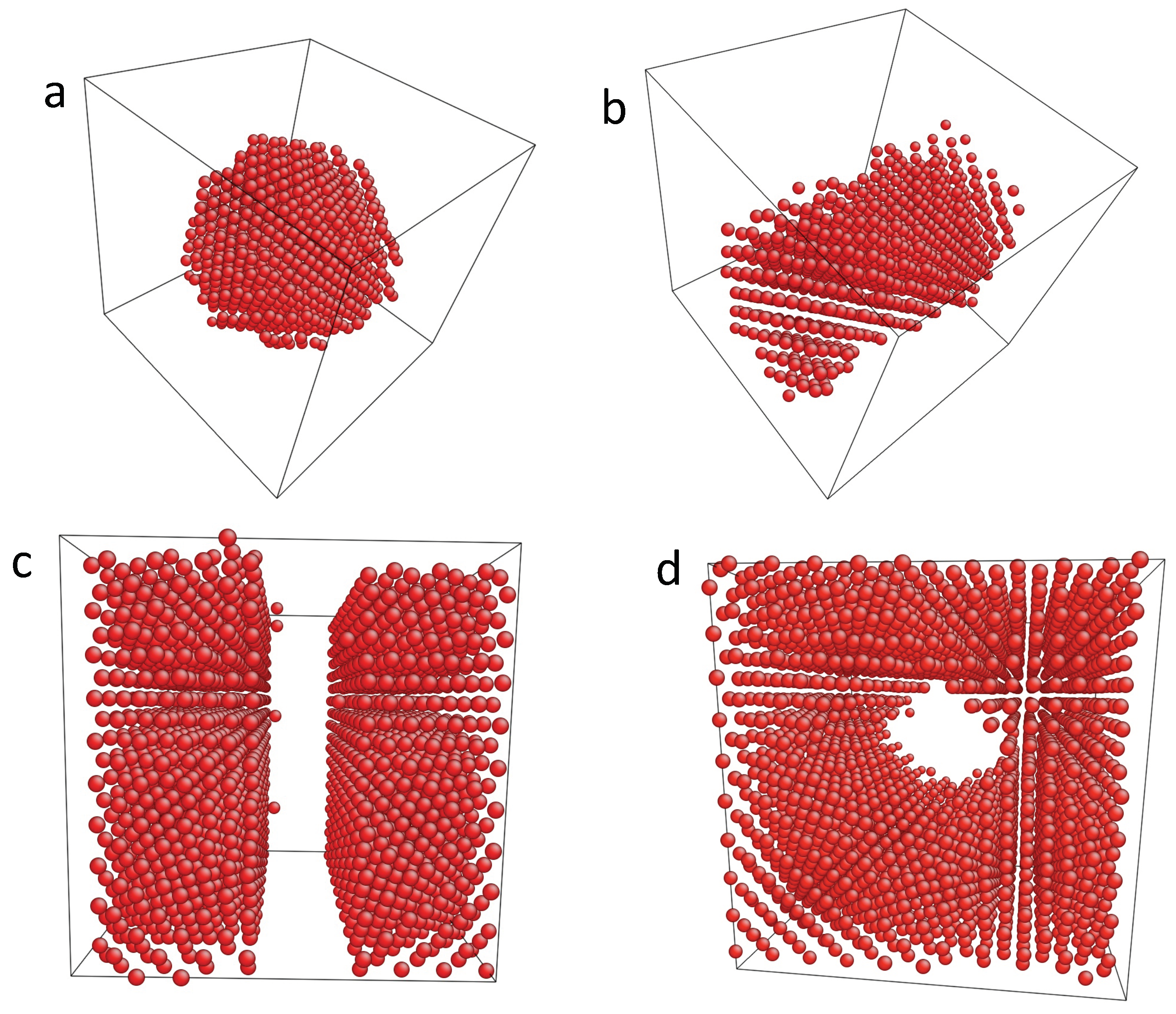
Figure 2.
Chemical potential of hydrogen as function of H concentration at . The S-shaped curve is the single phase prediction, the horizontal dashed line the Maxwell construction. For them, elastic effects are not taken into account, in contrast to the Monte Carlo data, which is for fixed volume (lattice constant of pure Ni). For high concentrations, compressive elastic effects become dominant. Apart from the dilute regions and , the Monte Carlo data correspond to two-phase configurations.
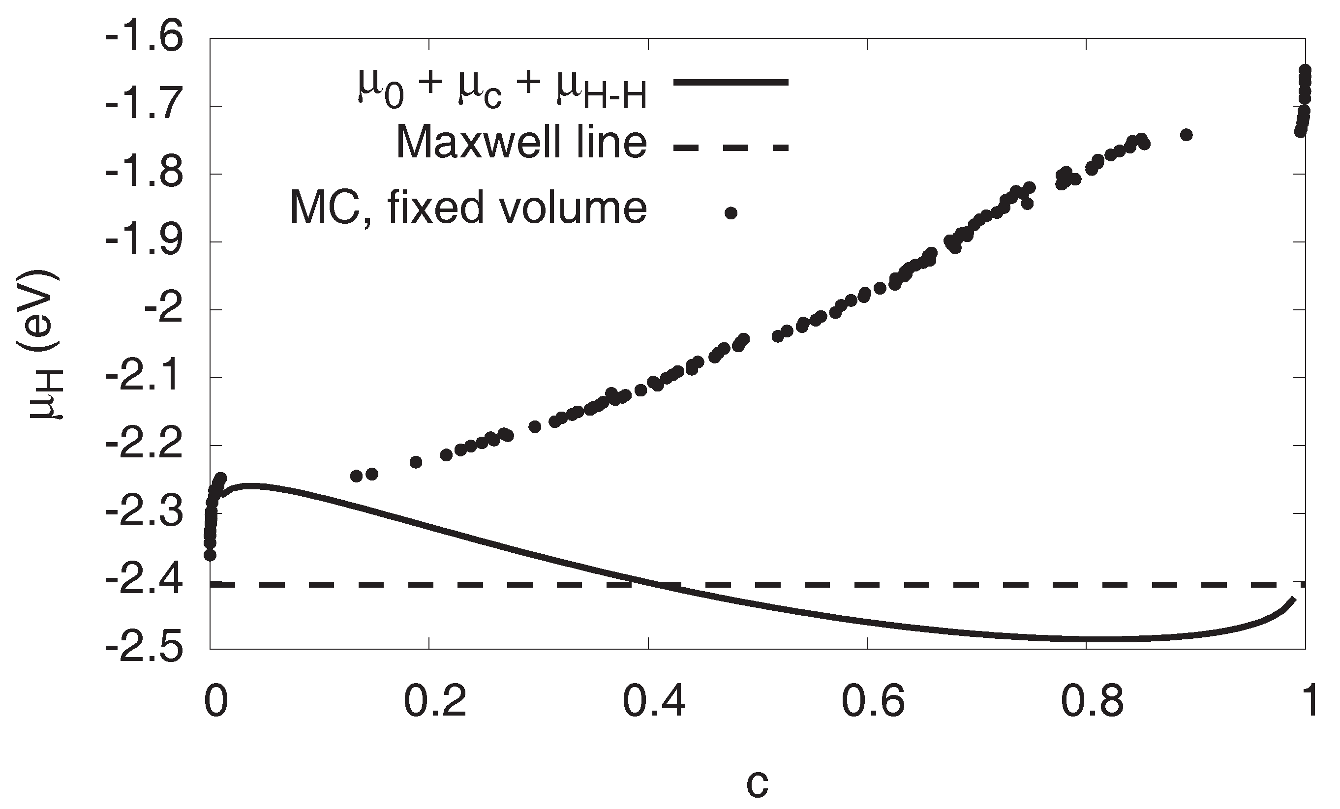
Figure 3.
Energy as function of the H concentration for a homogeneous and pressure free system, to determine the solvation energy and the H–H interaction. Notice that neither entropic effects are present at , nor elastic or interfacial effects. The Monte Carlo data is averaged over several configurations.
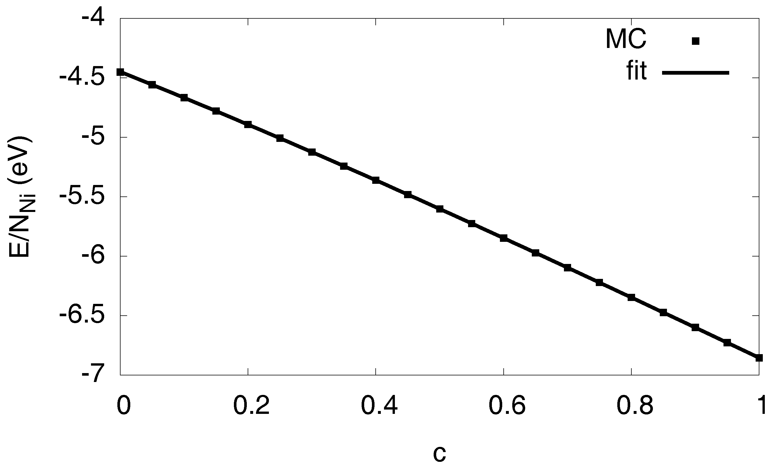
Figure 4.
The chemical potential contribution as function of the hydrogen concentration in a homogeneous system.
Figure 4.
The chemical potential contribution as function of the hydrogen concentration in a homogeneous system.

Figure 5.
Dilute limit of the chemical potential, which is dominated by the configurational entropy. The data are for and for fixed volume with the equilibrium lattice constant of pure Ni. The chemical potential is (apart from the offset ) dominated by the configurational contribution , whereas elastic and H–H interaction terms, and are negligible there. The accuracy of the continuum description in comparison to the Monte Carlo data are finally about 20 meV per atom in the entire concentration range .

Figure 6.
Chemical potential in the single phase state for different temperatures. The curves are the analytical descriptions based on the expression using the parameters of the H–H interaction and the solvation energy. The points are the data from the grand canonical Monte Carlo simulations of homogeneous, single-phase states. At low temperatures, the solubility is very low, and therefore the concentration range of the single phase equilibrium states limited to the dilute regions.
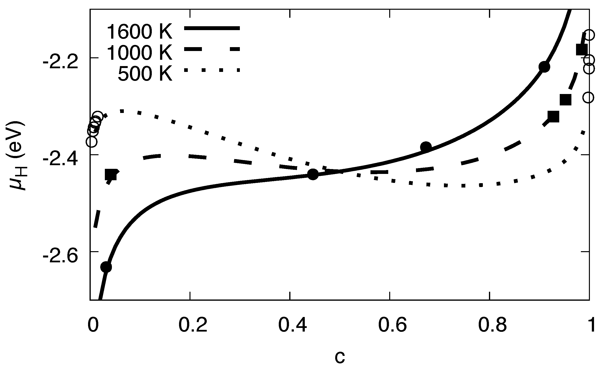
Figure 7.
Lattice constant as function of the hydrogen concentration. The Monte Carlo results are obtained from homogeneous free volume simulations, averaged over several configurations. The fit describes the nonlinear concentration dependence, in contrast to a linear interpolation (Vegard’s law).
Figure 7.
Lattice constant as function of the hydrogen concentration. The Monte Carlo results are obtained from homogeneous free volume simulations, averaged over several configurations. The fit describes the nonlinear concentration dependence, in contrast to a linear interpolation (Vegard’s law).

Figure 8.
Elastic contribution to the chemical potential in various approximations: The solid curve expresses the isotropic prediction by Equation (6), using equal elastic constants for both phases (we use the values of pure Ni). The long-dashed curve is the same isotropic model, but this time using the different elastic constants of both phases. This prediction is almost identical to a numerically calculated expression based on cubic elasticity, which assumes a spherical inclusion in a cubic box with periodic boundary conditions (short-dashed curve). In contrast to all these linear elastic approximations, the dotted line also considers elastic nonlinearities. Its prediction is very close to the Monte Carlo data.
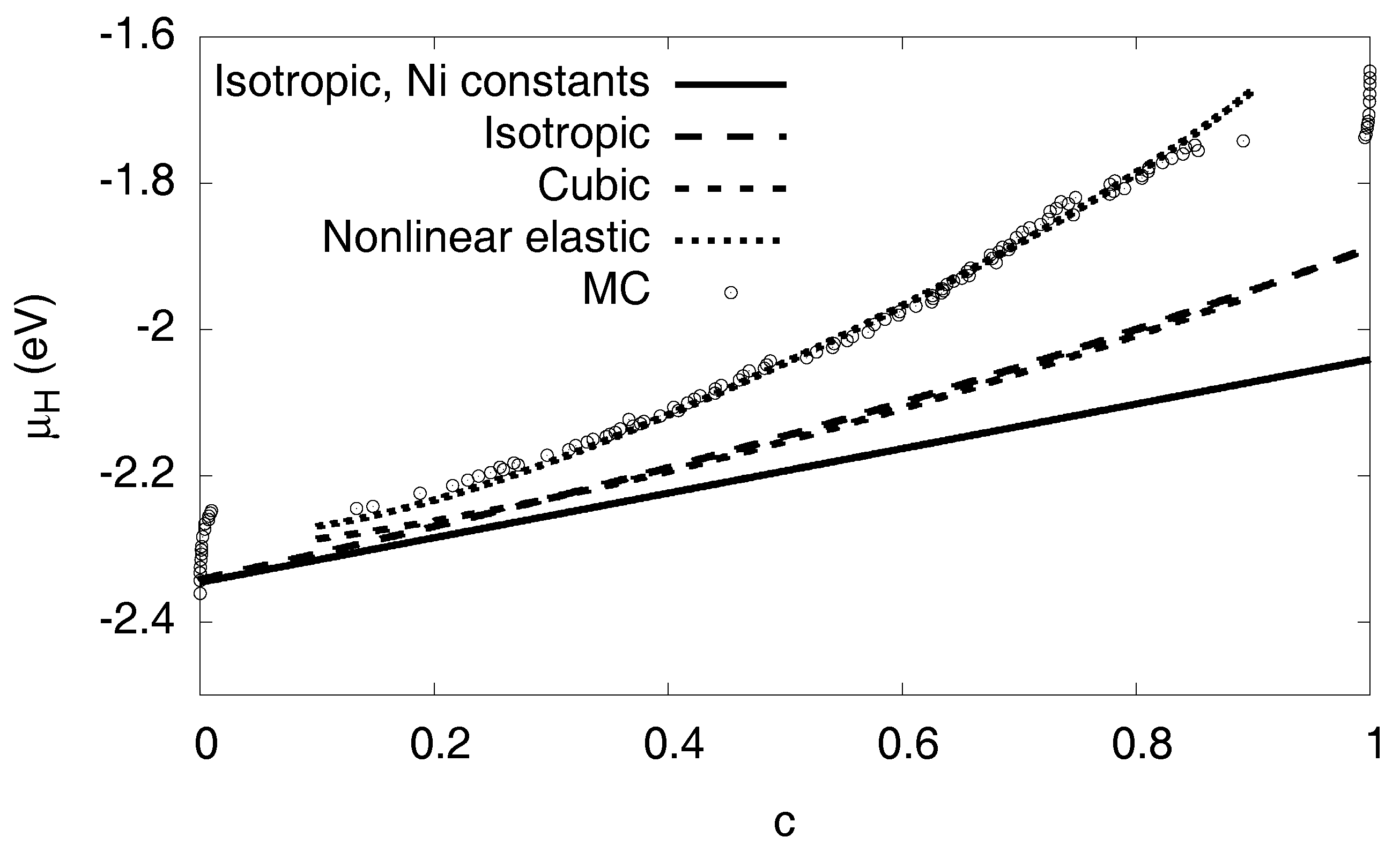
Figure 9.
Energy per Ni atom as function of the hydrogen concentration. The atomistic data are calculated at without Monte Carlo steps but atomic relaxation for fixed volume. A spherical precipitate is placed in the center to the simulation cell (with periodic boundary conditions). The irrelevant integration constant for pure Ni is subtracted, as well as the trivial term , thus only the H–H interaction, elasticity and surface contributions remain. The shape of the precipitate is not important for the elastic energy; we used both Ni-H and Ni inclusions in the atomistic simulation, visualized by open and filled spheres.
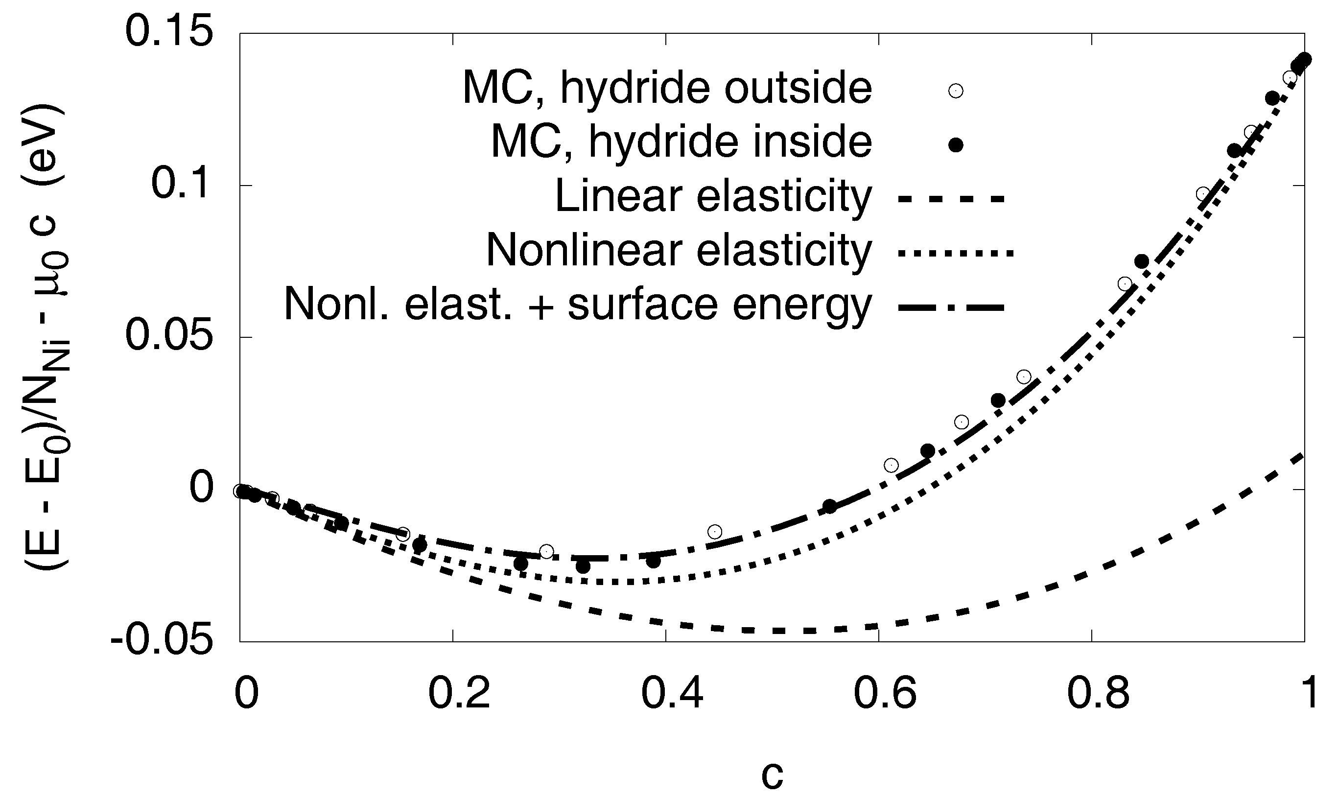
Figure 10.
The chemical potential of hydrogen at . The dots are the data from the Monte Carlo simulations. The chemical potential including nonlinear elastic effects is very close to the Monte Carlo data, and, together with interfacial effects, the agreement is excellent. The contribution from the interfacial terms is largest for low concentrations, as there the precipitates are small and therefore have the largest surface-to-volume ratio. The dotted curves near and are the analytical predictions for the single phase dilute limits. The H partial pressure is based on an ideal gas model, which is not realistic for higher pressures and only serves for illustrational purposes.

Figure 11.
Comparison of the chemical potential for fixed volume and in a stress-free situation, , . The volume constraint leads to a positive slope of the chemical potential in the two-phase region, thus stabilizing phase separation of given chemical potential. In contrast, two phase states are unstable for given , as shown here using the continuum prediction.

Figure 12.
Evolution of the hydrogen concentration as function of the number of Monte Carlo steps for . Grand-canconical simulations with given chemical potential are used. (Top) Fixed volume using the equilibrium lattice constant of Ni. Due to the positive slope of the chemical potential in the two-phase region (solid curve and data points in Figure 11) stable two phase states with arbitrary average concentrations can be obtained in thermodynamic equilibrium. (Bottom) For free volume, the miscibility gap is inaccessible for the given chemical potential in the grand canonical simulations, and instead the equilibrium state is almost free of hydrogen or almost fully saturated, as the solubilities are low at low temperatures (see phase diagram Figure 13). The reason for this behavior (which is accompanied by a hysteresis) is the negative slope of the chemical potential in the two-phase region (see Figure 11), which implies that these configurations are unstable. All simulations are started as a hydrogen free system, and formation of the hydride therefore demands to overcome a nucleation barrier.
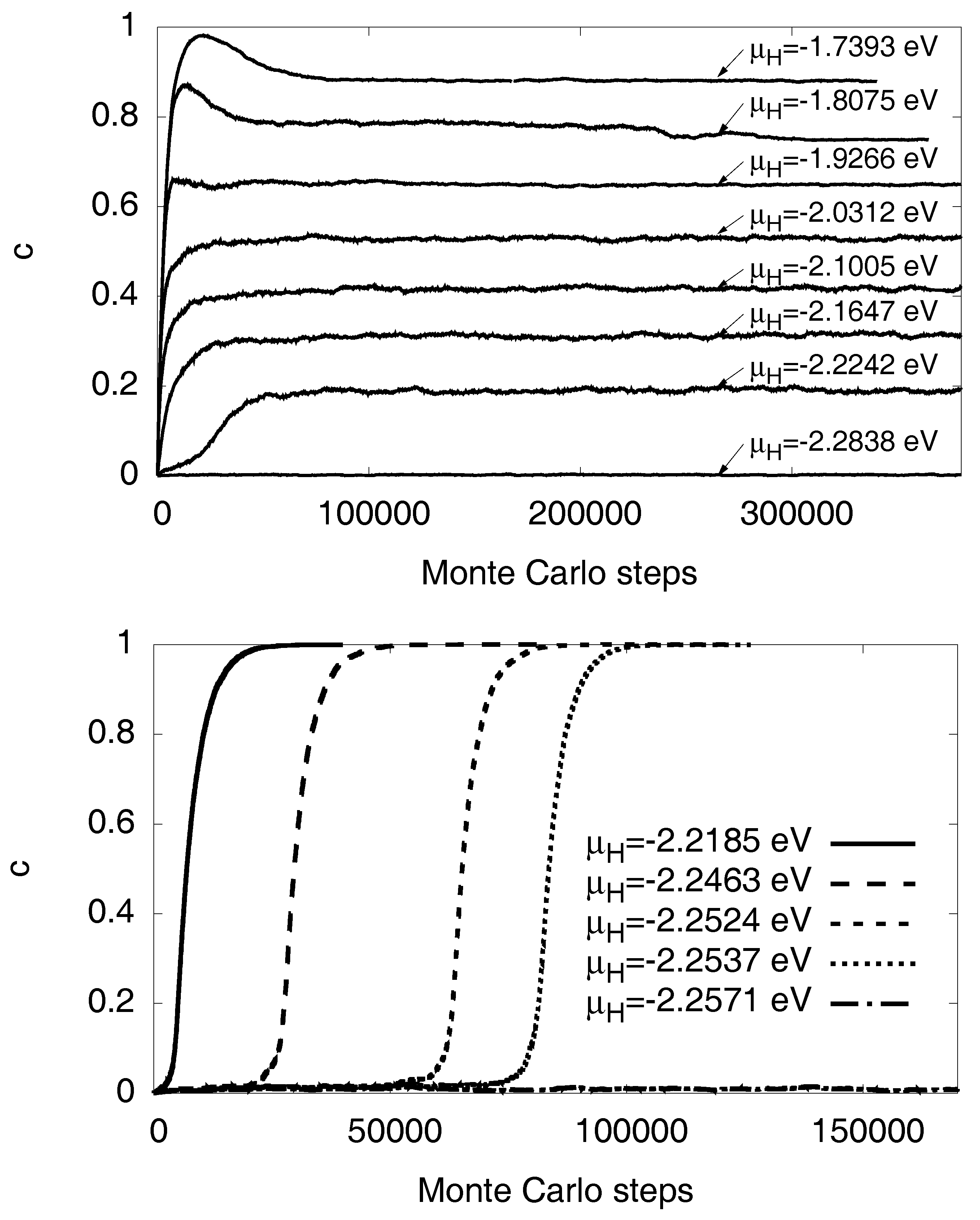
Figure 13.
Phase diagram of the Ni-H systems, based on parameters extracted from Monte Carlo simulations. The solid line is the binodal without consideration of elastic effects, whereas the dash-dotted line is the same with elastic effects for fixed volume.
Figure 13.
Phase diagram of the Ni-H systems, based on parameters extracted from Monte Carlo simulations. The solid line is the binodal without consideration of elastic effects, whereas the dash-dotted line is the same with elastic effects for fixed volume.

Figure 14.
Sketch of the hydride phase (light grey) forming as a slab in the nickel matrix with fixed volume. Due to translational invariance, we can assume the hydride phase to be located in the left part of the cube, starting at .
Figure 14.
Sketch of the hydride phase (light grey) forming as a slab in the nickel matrix with fixed volume. Due to translational invariance, we can assume the hydride phase to be located in the left part of the cube, starting at .
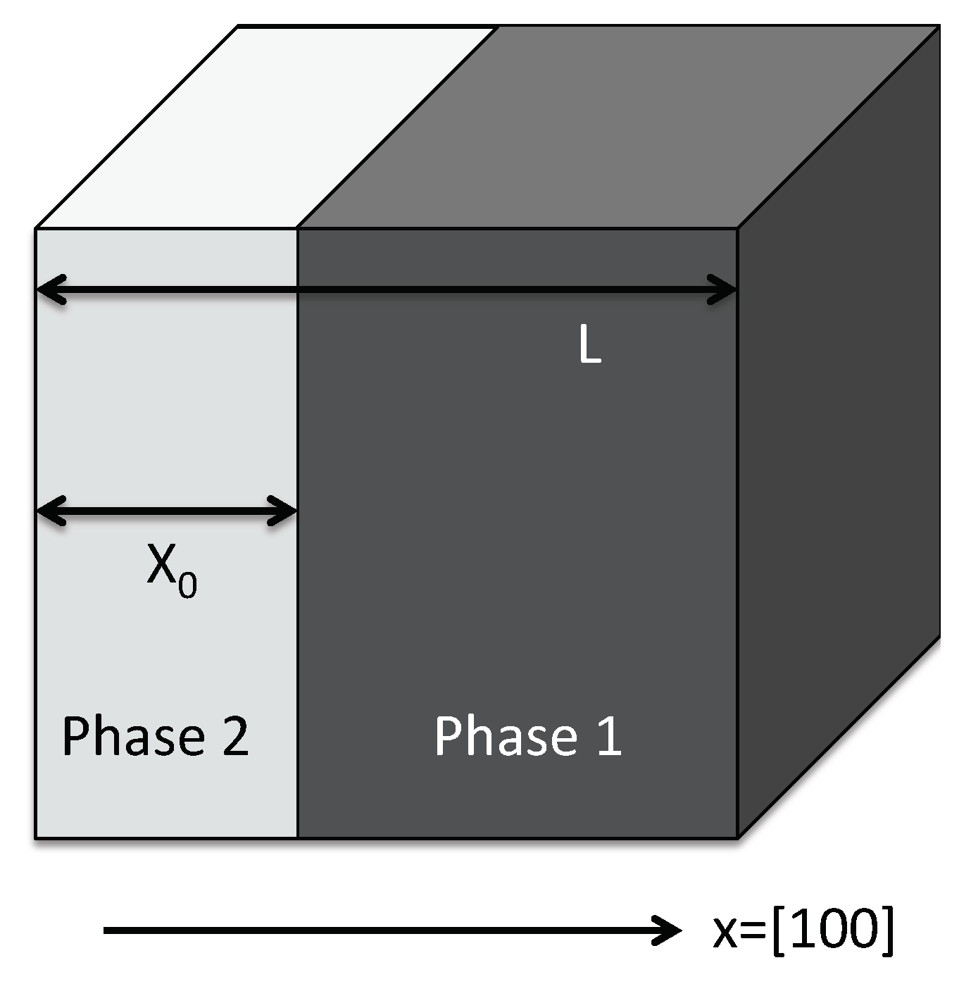
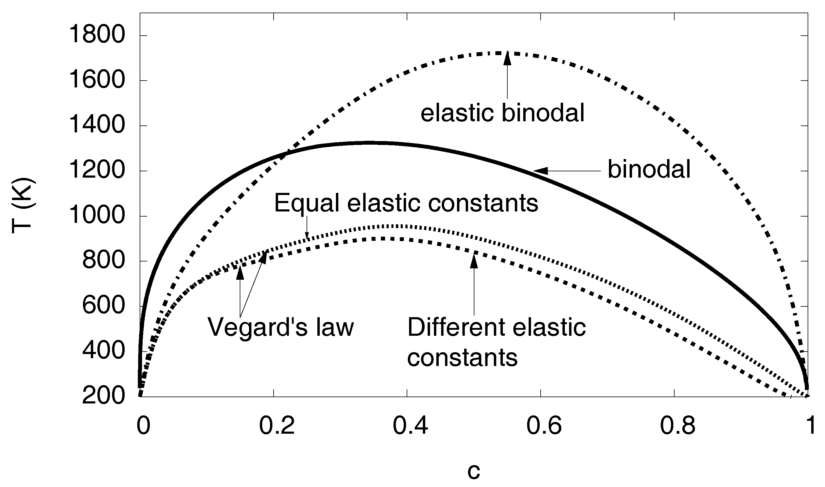
Figure 15.
The phase diagram depending on the eigenstrain is shown. The binodal and elastic binodal curves are the same as in Figure 13. The other two curves show the tremendous influence of the concentration dependence of the eigenstrain or lattice constant. If, instead of the concave dependence , a linear relationship is assumed (Vegard’s law), the solubility of hydrogen is drastically enhanced. In contrast, the concentration dependence of the elastic constants plays only a minor role: The case of different elastic constants anticipates a linear interpolation of the elastic constants between the values for Ni and Ni-H, whereas, for equal constants, both phases are assumed to have the same elastic constants (using values for Ni).

Table 1.
Elastic constants of pure nickel and the fully saturated hydride, as obtained from the EAM potential (see Appendix C for details). We note that the relaxed configuration of Ni is used as reference state.
Table 1.
Elastic constants of pure nickel and the fully saturated hydride, as obtained from the EAM potential (see Appendix C for details). We note that the relaxed configuration of Ni is used as reference state.
| Ni | Ni-H | |
|---|---|---|
| 250.7 GPa | 295.3 GPa | |
| 145.5 GPa | 197.3 GPa | |
| 134.3 GPa | 33.5 GPa |
Table 2.
Coefficients for the nonlinear elastic corrections. If higher order coefficients are missing, the expansion is truncated already at lower order.
Table 2.
Coefficients for the nonlinear elastic corrections. If higher order coefficients are missing, the expansion is truncated already at lower order.
| Elastic Constant | Material | |||||
|---|---|---|---|---|---|---|
| Ni | −3.25 | −7.04 | – | – | – | |
| Ni | −2.01 | −12.51 | – | – | – | |
| K | Ni | −1.00 | 0.53 | −4.49 | 2.57 | 50.03 |
| Ni-H | −22.80 | −47.20 | – | – | – | |
| Ni-H | −9.77 | −14.69 | – | – | – | |
| K | Ni | −2.25 | 3.37 | 11.51 | 3.55 | −51.00 |
© 2018 by the authors. Licensee MDPI, Basel, Switzerland. This article is an open access article distributed under the terms and conditions of the Creative Commons Attribution (CC BY) license (http://creativecommons.org/licenses/by/4.0/).
Share and Cite
MDPI and ACS Style
Korbmacher, D.; Von Pezold, J.; Brinckmann, S.; Neugebauer, J.; Hüter, C.; Spatschek, R. Modeling of Phase Equilibria in Ni-H: Bridging the Atomistic with the Continuum Scale. Metals 2018, 8, 280. https://doi.org/10.3390/met8040280
AMA Style
Korbmacher D, Von Pezold J, Brinckmann S, Neugebauer J, Hüter C, Spatschek R. Modeling of Phase Equilibria in Ni-H: Bridging the Atomistic with the Continuum Scale. Metals. 2018; 8(4):280. https://doi.org/10.3390/met8040280
Chicago/Turabian StyleKorbmacher, Dominique, Johann Von Pezold, Steffen Brinckmann, Jörg Neugebauer, Claas Hüter, and Robert Spatschek. 2018. "Modeling of Phase Equilibria in Ni-H: Bridging the Atomistic with the Continuum Scale" Metals 8, no. 4: 280. https://doi.org/10.3390/met8040280
Note that from the first issue of 2016, this journal uses article numbers instead of page numbers. See further details here.