Characterization of Austenite Microstructure from Quenched Martensite Using Conventional Metallographic Techniques and a Crystallographic Reconstruction Procedure

Abstract

Recently, procedures for recovering austenite fcc crystallographic information from EBSD (Electron Back-Scatter Diffraction) data recorded from martensite or other bcc transformation products have been proposed. Due to the difficulties in revealing prior austenite grain boundaries using available etching techniques, these reconstruction methods appear as promising tools for understanding austenite hot deformation behavior in low carbon steels. In a previous work, the accuracy of an in-house developed reconstruction code was validated using an Fe-30Ni alloy. Validation of this method in low carbon steels is more difficult due to the loss of austenitic orientation information. In addition, it is not known how the results of conventional metallography correlate with those of the reconstruction or which scan parameters or post-processing treatments are necessary for obtaining comparable results. To study this, two martensitic specimens obtained from water quenched recrystallized and deformed austenite were characterized in this study, using both conventional metallographic techniques and the above mentioned reconstruction procedure applied to EBSD scans acquired using different parameter values. The comparability of austenite grain size and morphology was analyzed as a function of the post-processing treatment. The results show that in order to obtain comparable results, it is critical to analyze the coherence of the twins present in the microstructure.

1. Introduction

In recent decades, the evolution of austenite microstructure during hot deformation in low carbon steels has been widely studied. Grain size, strain accumulation levels, and the crystallographic orientation of austenite before phase transformation can all affect the final room temperature microstructure of the steel [1,2,3] and, correspondingly, the properties of the final product. Therefore, knowledge of the austenite microstructure evolution during hot deformation is required in order to aim to improve the parameters of the thermomechanical control process (TMCP). Very often, indirect methods such as the analysis of strain-stress curves are used to characterize austenite hot deformation behavior [4,5]. The characterization of the austenite in carbon steels is especially difficult due to phase transformation during cooling. Although several etching techniques have been developed to reveal the austenite microstructure from quenched martensite [6,7], they are often ineffective, mainly in the case of low carbon steels [8]. Moreover, their ability to reveal some special grain boundaries is questionable [9,10], and important information regarding the crystallography and texture of the parent phase cannot be recovered.

Recently, methods for reconstructing the austenite orientation information from transformed microstructure orientation maps measured by Electron Back-Scatter Diffraction (EBSD) have appeared as powerful tools to characterize the austenite. Crystallographic reconstruction was first successfully applied by Humbert et al. [11,12,13] for Ti and Zr alloys undergoing the bcc to hcp β → α phase transformation. Although it is more difficult, several reconstruction methods have been reported for recovering austenite crystallographic data from EBSD data on bcc microstructures [9,10,14,15,16,17,18]. All these methods take the crystallographic correspondence between the parent grain and transformed product as their basis in terms of an orientation relationship. In all cases, the nucleation and growth of the new phase must take place inside the same austenite grain, as this is the case for displacive phase transformations.

Some studies have shown that applying the reconstruction method leads to realistic results in several steels [9,16], while other studies on other steels have determined a good correlation between the orientation of retained austenite islands in bainitic microstructures and the reconstructed grains [9,10,14,15]. In a previous study [18], we focused on the validation of a reconstruction code based on the one proposed by Germain et al. [10] in an Fe-30Ni alloy, which is particularly suited for this task since after water quenching the material presents an fcc austenitic microstructure which can transform to martensite after subzero quenching. It was therefore possible to apply the reconstruction procedure to the martensitic crystallographic data obtained by EBSD and to compare the results with the original crystallographic fcc data obtained on the same area of the specimen.

However, there are still open questions that need to be resolved before the reconstruction procedure can be used to characterize austenite microstructures in low carbon steels and before the results can be incorporated into the existing microstructural evolution models. Validating reconstruction results in these steels is more difficult due to the loss of austenitic crystallographic orientation information. In addition, one must take into account that, thus far, the austenite morphologies and grain sizes which serve as input or output data for austenite microstructural evolution models have been characterized through indirect metallographic techniques, mainly an etchant consisting of an aqueous solution of picric acid and a wetting agent [19,20,21]. Germain et al. [10] and Bernier et al. [9] showed examples of the comparison between the reconstructed boundaries and the results of this type of metallographic characterization. Although a good correspondence was determined in both cases, it was found that not all of the boundaries present in the reconstructions were revealed by the etching procedure. However, this was not analyzed in detail, and quantitative results were not provided. Although, in a recent work [22], the results of the code developed by Cayron et al. [14] have been compared with conventional metallographic techniques, there is little knowledge on how the grain sizes determined by both techniques correlate. In addition, there is little information available on the EBSD scan setup, reconstruction parameters or reconstruction post-processing procedure necessary to obtain comparable data.

In this article, EBSD scans were performed using different step sizes and scan areas on two water quenched martensitic low carbon samples that were obtained from recrystallized and deformed austenite microstructures, respectively. The procedure described in [18] was applied to the EBSD scans to reconstruct the austenite crystallographic information. Next, the specimens were etched in an aqueous solution of picric acid and then characterized using optical microscopy. The morphology of the grain boundaries revealed by picric acid and the grain sizes measured by conventional metallography were compared with the results of the reconstruction using different criteria to define grain boundaries.

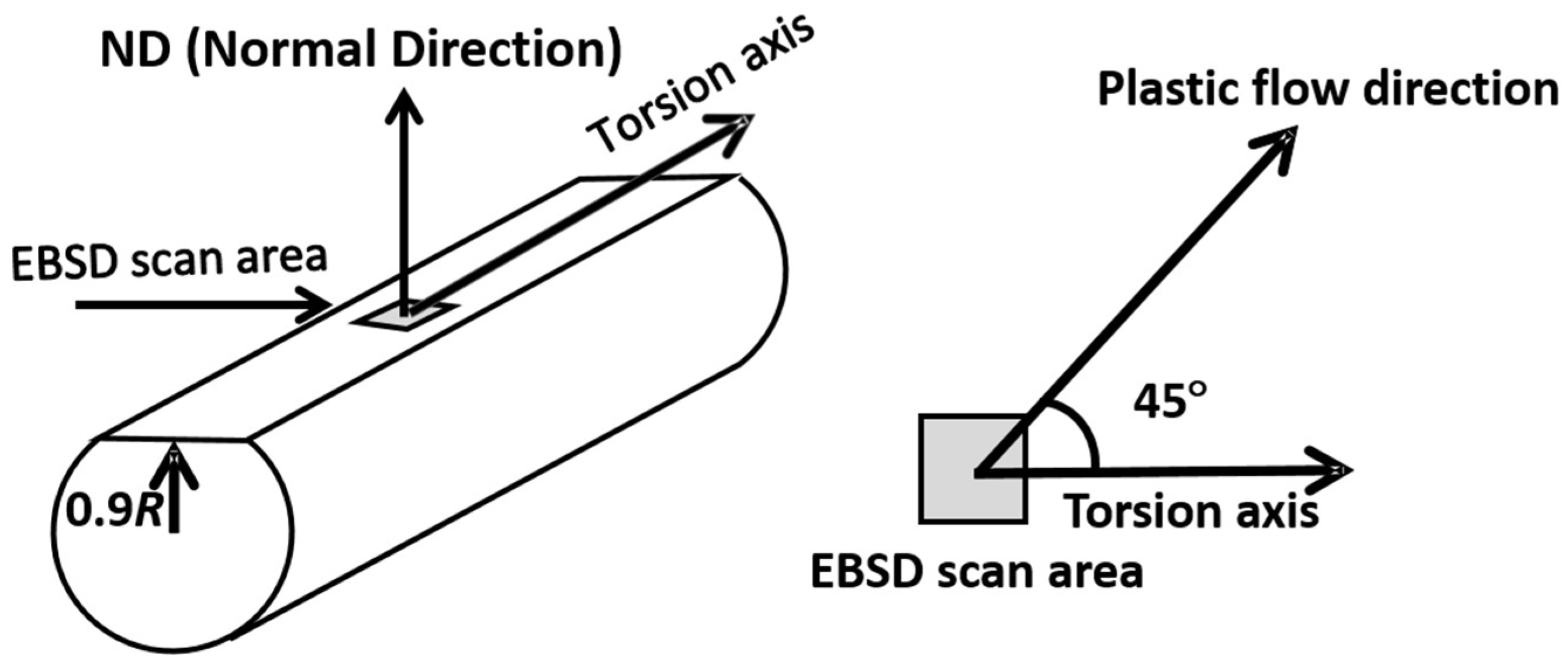
2. Materials and Methods

Two steels, Al1 and Al1Nb3, whose compositions are given in

Table 1. Composition of the steels investigated in the present work (wt %).

Steel	C	Mn	Si	P	S	Al	Cu	Cr	Ni	Nb	Ti	N
Al1	0.21	2.0	0.01	0.02	0.001	1.06	<0.005	<0.005	<0.005	0.001	0.001	0.005
Al1Nb3	0.21	2.0	0.01	0.02	0.001	0.88	<0.005	<0.005	<0.005	0.028	0.001	0.004

, were investigated in this study. Both steels had been previously analyzed [19,23,24] as part of a project on the effect of high Mn, Si and Al addition levels on the hot deformation behavior of low carbon steels [25], and they were selected for the present study due to the fact that they present a good etching quality in revealing the previous austenite grain boundaries from quenched martensite. Most of the analysis was carried out on a recrystallized sample of Al1 steel produced in an interrupted torsion test. The torsion specimen consisted of a gauge geometry that was 7.5 mm in diameter and 16.5 mm in length. The applied thermomechanical cycle included a reheating treatment at 1250 °C for 15 min, followed by a cooling down to 950 °C, where a deformation pass ($\epsilon$ = 0.35, $\dot{\epsilon }$ = 1 s⁻¹) was applied and the specimen was held at this temperature for 185 s. This duration was calculated so as to obtain a statically recrystallized microstructure based on previous double-hit torsion tests [19]. After the holding time, the specimen was water quenched. A deformed Al1Nb3 specimen was also analyzed. This specimen was also produced in torsion, following a multipass deformation sequence based on a hot rolling schedule to produce a plate with a final thickness of 50 mm [19,25]. The sequence includes four deformation passes to simulate roughing (deformation temperatures from 1200 °C to 1149 °C and six deformation passes to simulate finishing (deformation temperatures from 927 °C to 860 °C), followed by water quenching to produce a martensitic microstructure. After finishing, a deformation accumulation level of approximately ε ≅ 0.8 was obtained. Detailed information on the deformation sequence can be found in Table 6 of Reference [19] (930 °C-50 mm schedule).

After being water quenched, both specimens were prepared for EBSD and metallographic analysis. The characterization was carried out on the sub-surface section, which corresponds to 0.9 times the outer radius of the torsion specimen (see the experimental setup in Figure 1). For the EBSD analysis, the samples were prepared by using standard mechanical polishing procedures that ended with a polishing step in a colloidal silica solution. Orientation imaging was performed using a FEG-SEM JEOL JMS 7100F (Jeol Ltd., Tokyo, Japan) equipped with a NORDLYS II camera and HKL Channel 5 operating at 10 kV. In the case of the recrystallized Al1 martensitic sample, three EBSD maps were acquired using a square grid, using step sizes 0.5 μm, 1 μm and 1.5 μm and scan areas from 350 × 350 to 900 × 900 μm². The time for scan acquisition was approximately similar in the three cases (≅12 h), and the scan areas were adjusted as a function of the step size, keeping the rest of the scan parameters constant. In the case of the deformed Al1N3 specimen, one single EBSD scan using a step size of 1 μm and an area of 500 × 500 μm² was performed. Standard grain dilation cleaning procedures were applied to the scan data obtained from the martensitic microstructure. TSL OIM Analysis 5.31 [26] software (EDAX, Mahwah, NJ, USA) was used to perform all post-processing of scans and of the reconstruction crystallographic data obtained from an in-house developed method [18] and from reconstruction data. After each scan, the specimens were prepared again using conventional metallographic techniques, etching in a picric acid water solution with a wetting agent (Bechet–Beaujard etching [6]) to reveal the austenite grain boundaries, and examined using optical microscopy. In the case of the recrystallized sample, the grain boundaries revealed by etching were traced manually and converted into a jpg image using the GIMP program (2.8.14, http://www.gimp.org/) [27]. Next, using LAS v.45 [28] software (Leica Microsystems, Wetzland, Germany), the area of each grain was calculated and then an equivalent diameter was assigned to each grain, which was the diameter of the circle with an equal area. The average of all the diameters measured is known as the mean equivalent diameter (MED).

3. Results

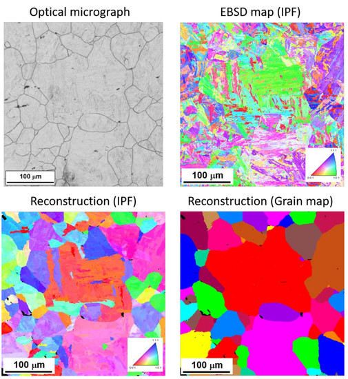
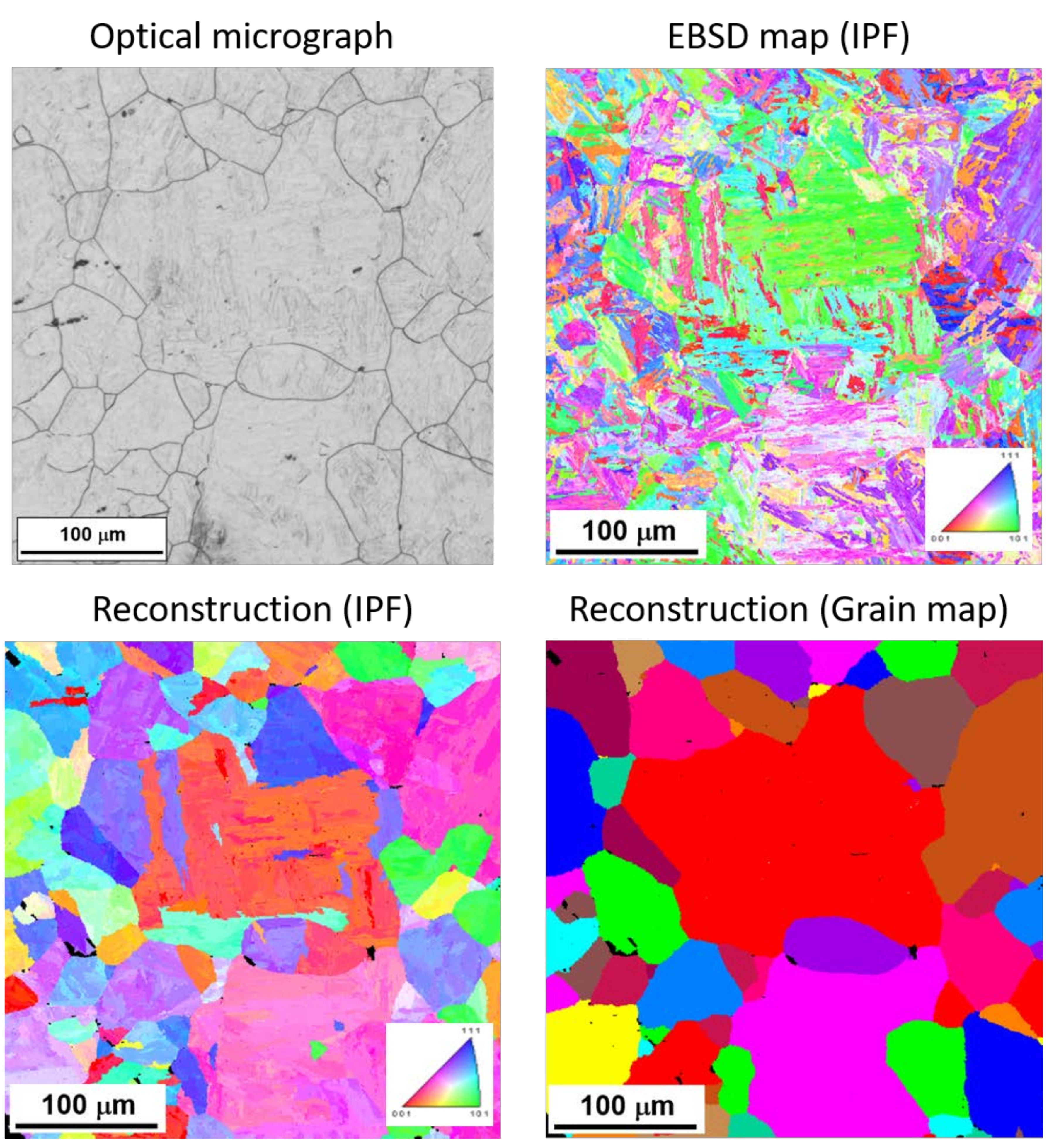
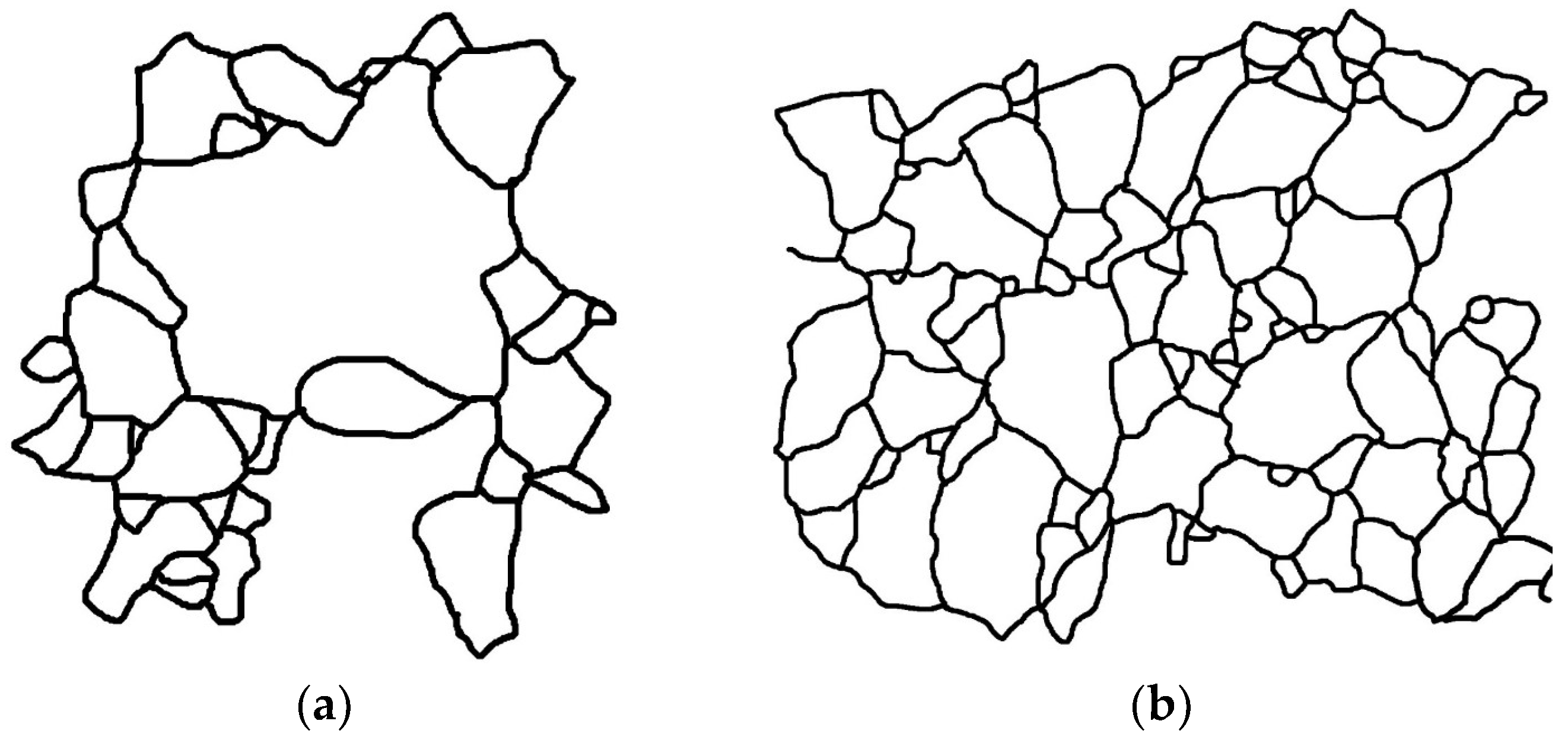
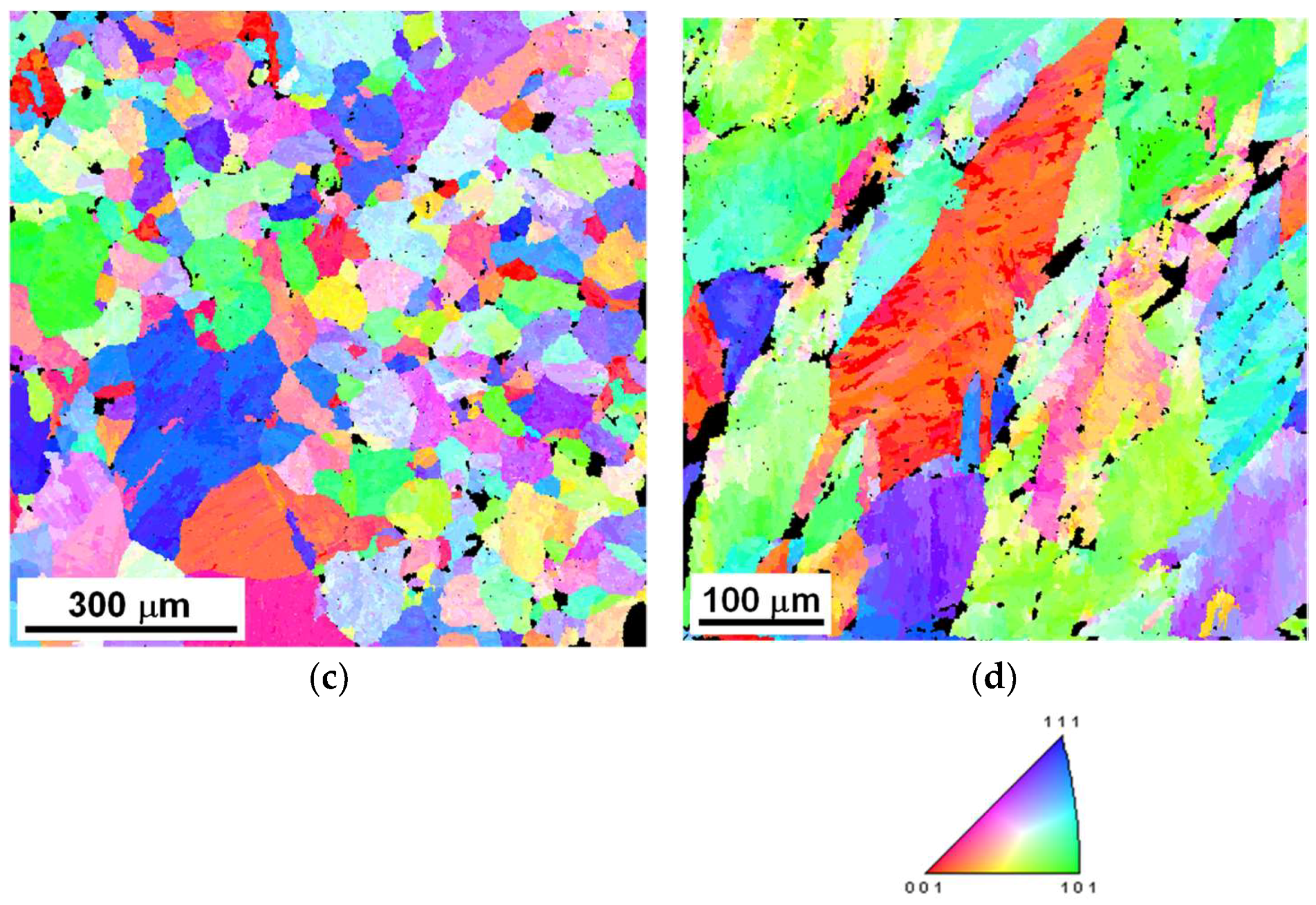
3.1. Microstructural Characterization

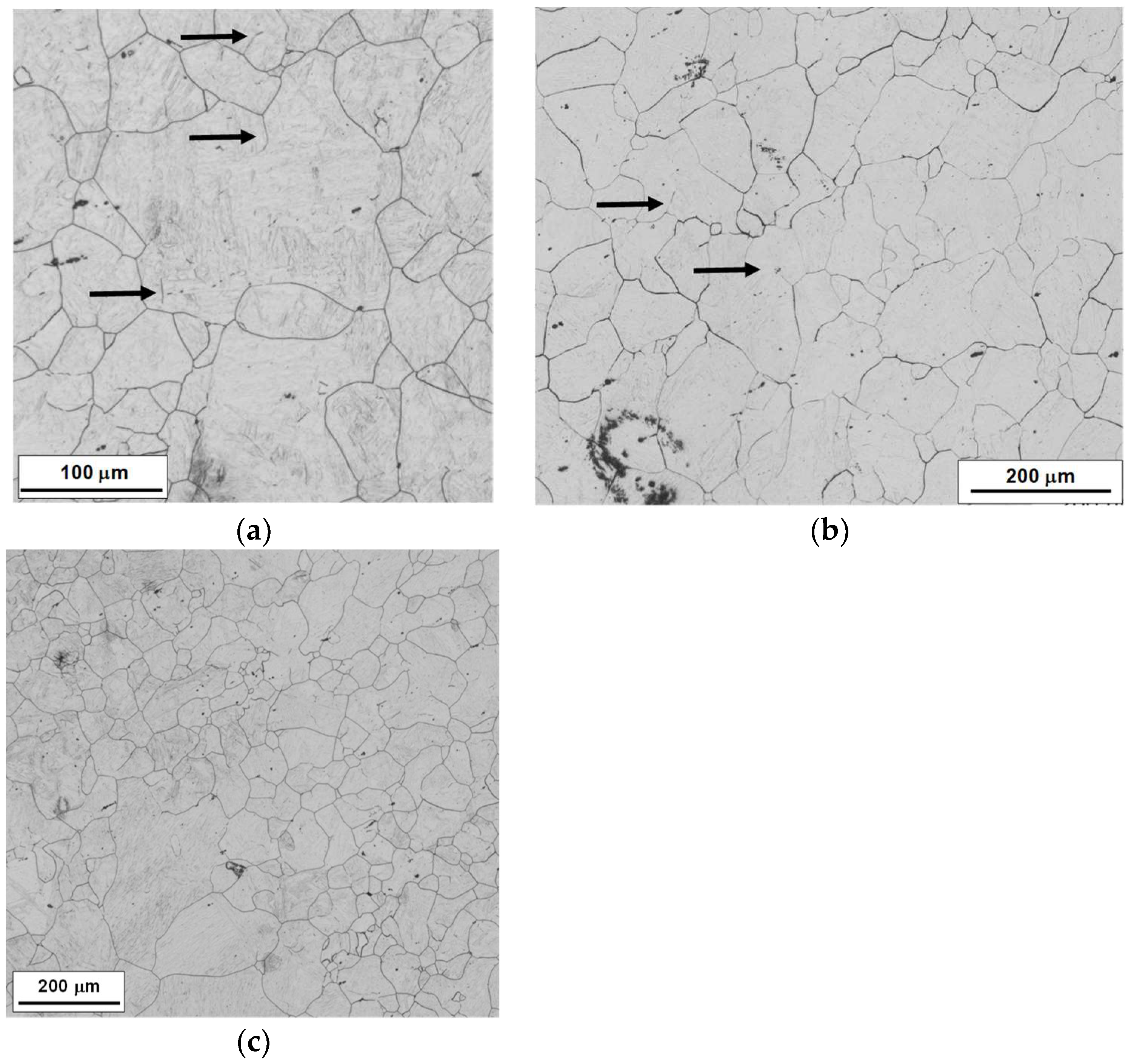
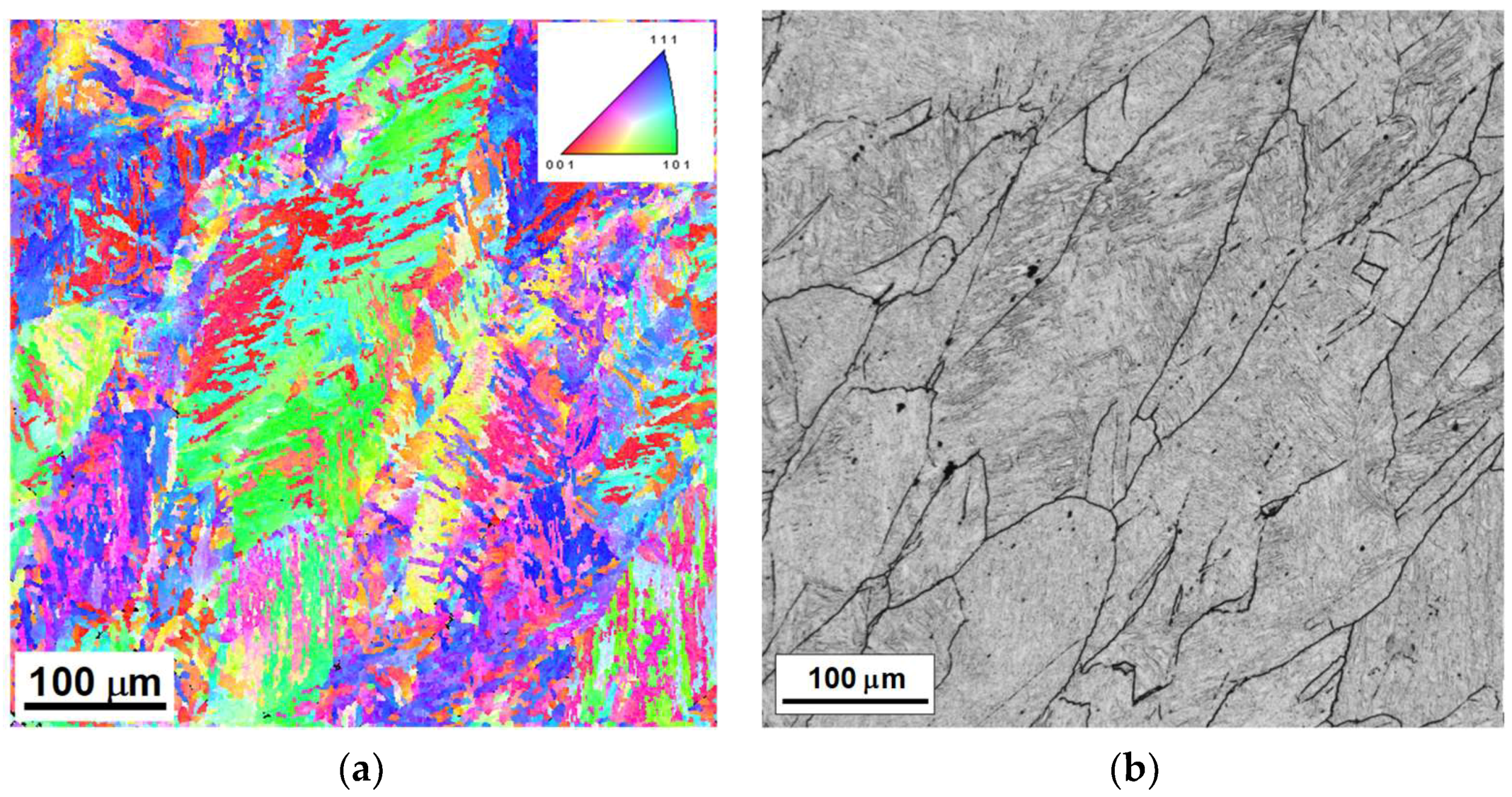
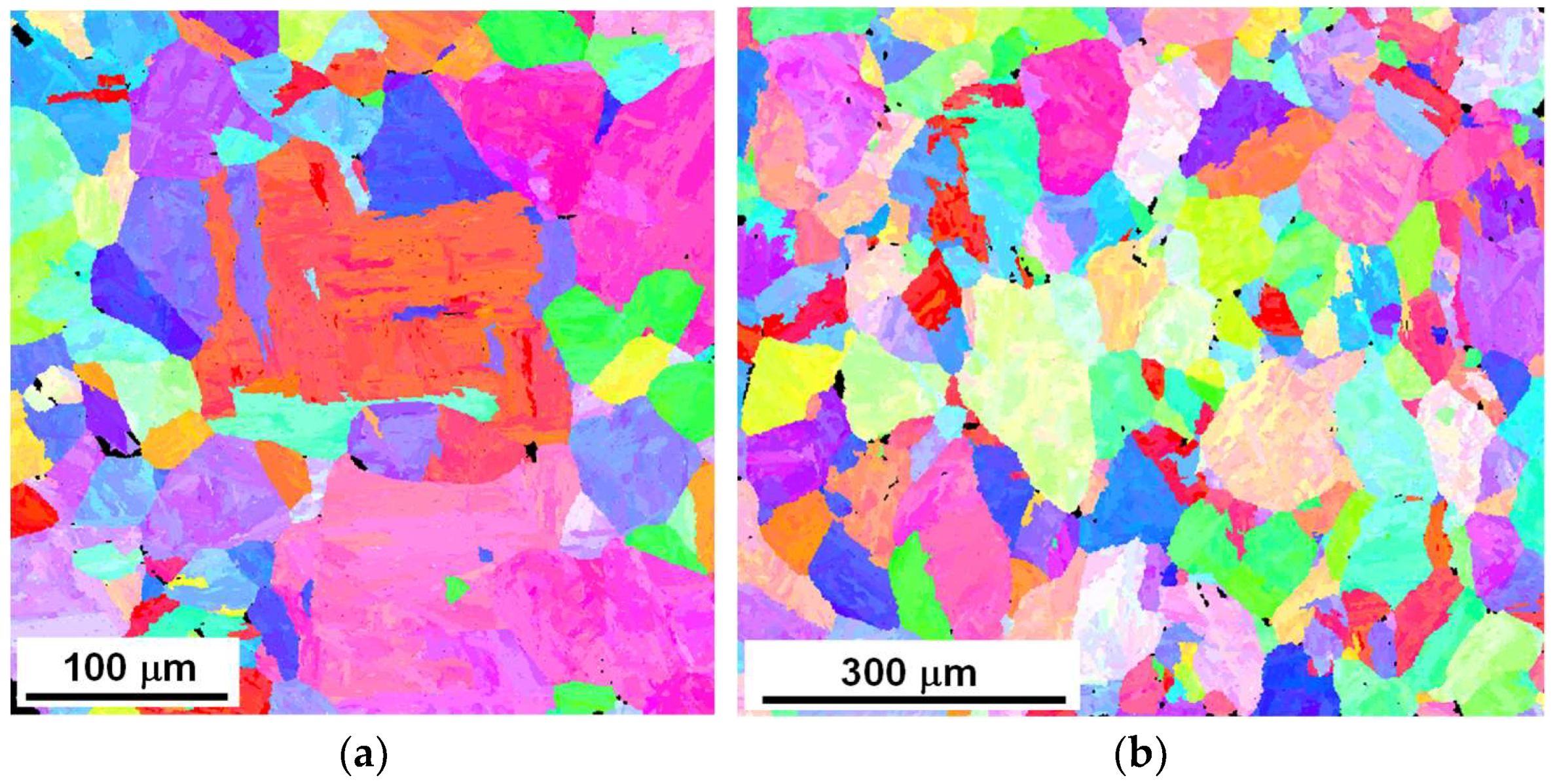
3.1.1. Recrystallized Microstructure

Figure 2 shows the ND (Normal Direction, see Figure 1) inverse pole figure (IPF) maps obtained from the martensitic sample quenched from recrystallized austenite using different step and scan sizes; in Figure 3, the optical micrographs of approximately the same areas obtained after etching with picric acid are represented. Figure 2 shows that as step size decreases, the martensitic microstructure can be characterized with greater detail, although a smaller area is analyzed when using similar scan acquisition times. After the sample is etched with picric acid, a microstructure of approximately equiaxed grains is revealed. Although the etching quality is good in all three cases, slightly better results can be observed in the case of Figure 3a,c. Some microstructural heterogeneity is also evident in these two micrographs. The same phenomenon was observed in the initial microstructure obtained after soaking at 1250 °C (average and maximum grain sizes were 98 and 513 μm, respectively), and as shown in the micrographs, this heterogeneity was not removed after deformation and full recrystallization at 950 °C.

It can also be noted from Figure 3 that, after etching, some of the boundaries show a weaker contrast, and that in some cases they do not close to define grains (see examples marked by arrows in Figure 3a,b). As a result, some ambiguity in the grain size determination can be expected. For clarity, the sketches used for grain size measurements from the optical micrographs have been included in Figure 4, together with the MED results for the three optical micrographs. As shown in the picture, the grains that make contact with the outer border of the micrograph were excluded from the measurement. The smallest average grain size was obtained in the case of Figure 3a, MED = 33.6 ± 11.0 μm. This can be attributed to the small area selected for analysis, which leads to a low number of grains (34) contributing to the measurement and to the exclusion of some of the coarsest ones as border grains. In the case of Figure 3b,c, larger average values, MED = 54.6 ± 7.8 μm and MED = 46.7 ± 4.4 μm, respectively, were determined, and the number of grains measured increased to 87 and 229 grains.

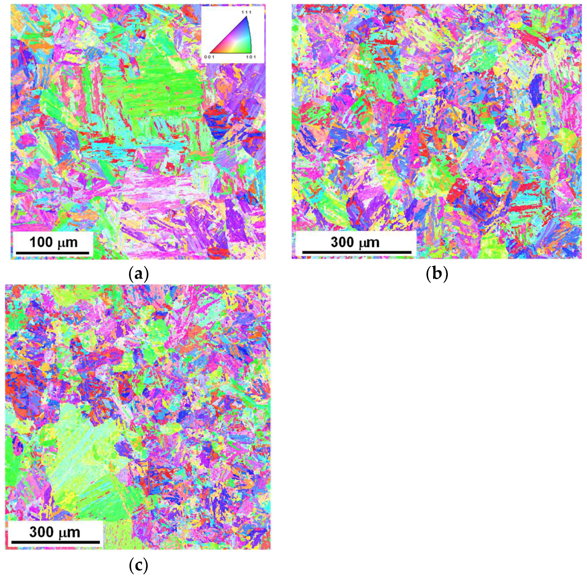
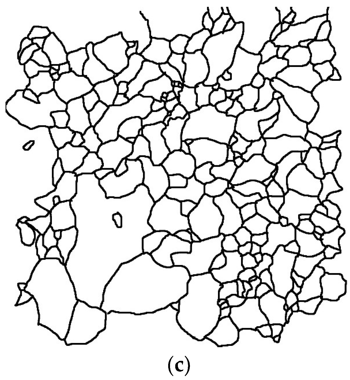
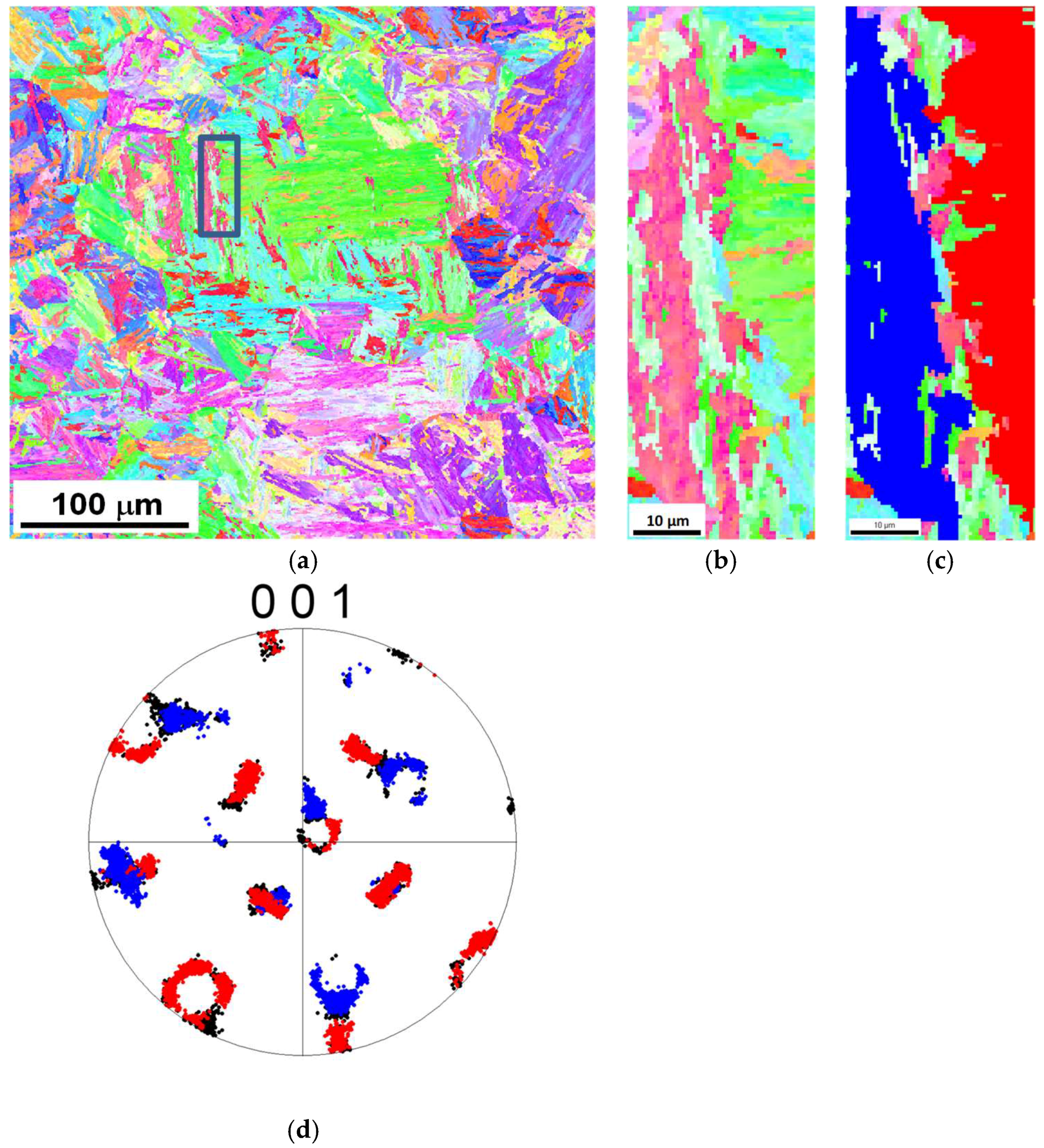
3.1.2. Deformed Microstructure

Figure 5a shows the IPF ND map obtained from the martensitic sample quenched from deformed austenite. The corresponding optical micrograph obtained from the same area after picric acid etching is shown in Figure 5b. The optical micrograph shows that, as expected from the deformation schedule, before quenching a pancaked austenite microstructure was produced. Although some of the grain boundaries are only partially revealed, Figure 5b mainly shows deformed austenite grains elongated in the plastic flow direction. In addition, the optical micrograph shows boundaries whose morphology appears to be delineating twins or other features related to the deformation microstructure.

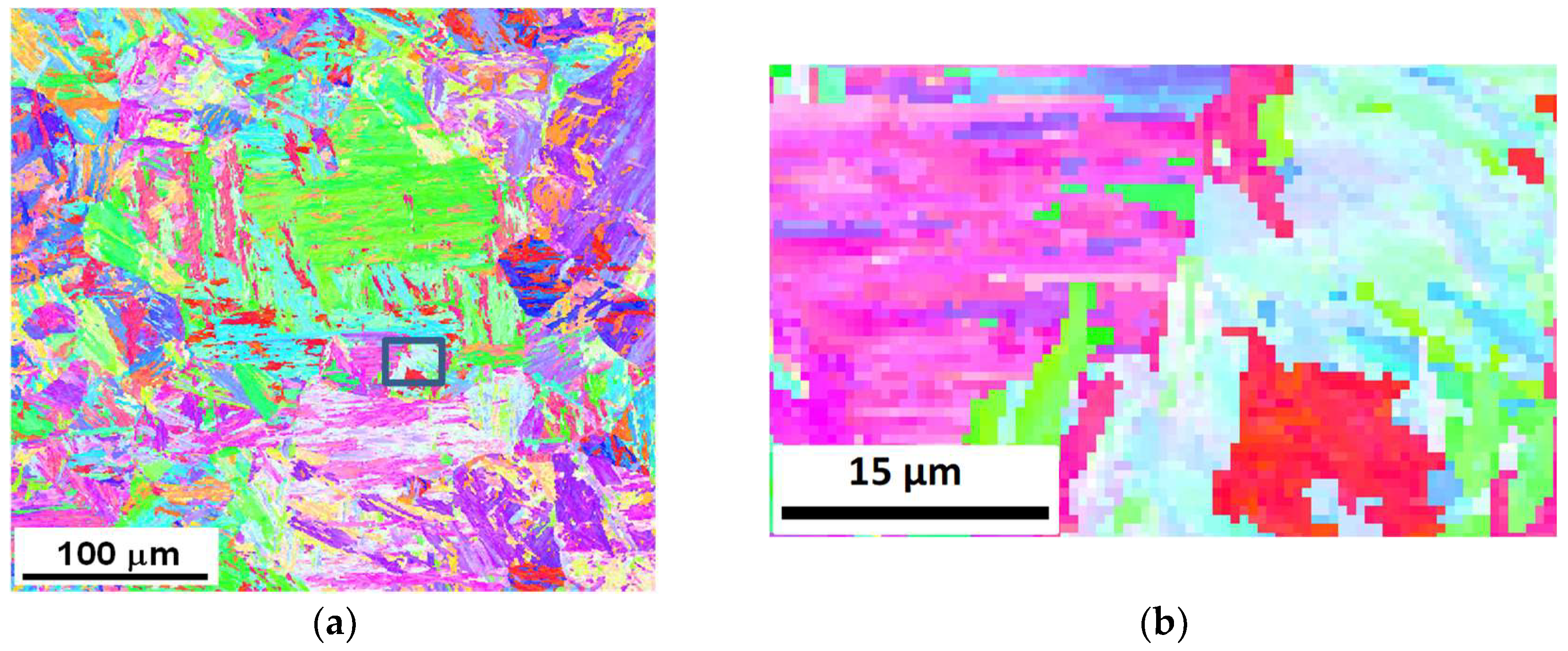
3.2. Application of Reconstruction Procedure

The reconstruction model employed in this article is a fully automated in-house code developed at Ceit using MATLAB (Release 2013b, The MathWorks Inc., Natick, MA, USA) [29]. A detailed description of the program and reconstruction parameters can be found in Reference [18]. The program is mainly based on the principles of the parent austenite reconstruction approach proposed by Cayron et al. [14] and Germain et al. [10] for the fcc to bcc γ → α phase transformation in steels and previously developed for the bcc to hcp β → α phase transformation for Ti and Zr alloys by Humbert et al. [11,12,13]. The original crystallographic data are first treated and divided into crystallographic domains, which are defined as sets of adjacent pixels misoriented from neighbor to neighbor at less than a critical angle, $\mathsf{\theta }$ [10]. The reconstruction procedure is divided into two steps: “γ nuclei identification” and “γ nuclei spreading”. In the “γ nuclei identification” routine, the code takes all the bcc crystallographic domains and compares their average orientations with those corresponding to their neighbors. The objective is to identify parent orientations which are consistent with the majority of the domains (within a tolerance angle ${\omega }_0$) and exclude the rest from the solution. The calculated austenite parent orientations are considered valid if a minimum number of different bcc orientations, $N_v$, is contributing to the solution, and if the ratio between the number of neighbor domains contributing to the most probable solution and the number of neighbors contributing to the second most probable solution is higher than a given value. In the next routine, “γ nuclei spreading”, the code seeks to assign an fcc orientation to those domains which were not identified during the previous step through a comparison with the austenite orientations already calculated for neighboring domains, using a tolerance angle ${\omega }_1$. More detailed information about the procedure can be found in Reference [18].

The effect of the different parameters on the reconstruction performance was discussed in a previous work [18]. It was observed that the efficiency of the code decreased significantly when using the Kurdjumov-Sachs orientation relationship. However, similar results were obtained when the Greninger-Troiano, Miyamoto [16] or an optimized orientation relationship were employed. Therefore, the orientation relationship reported by Miyamoto et al. [16] for a low 0.15% C steel was employed here. For the rest of the parameters, values that lead to a good reconstruction performance for recrystallized microstructures were applied: $\mathsf{\theta }=3.5°$, $N_v=4$, $PR=1.5$, ${\omega }_0=3.5°$, and ${\omega }_1=8°$ [18].

Figure 6 shows IPF ND maps obtained from the reconstructed austenite. It can be observed that in the four cases large reconstructed area fractions were obtained (>95%). The lowest reconstructed area fraction corresponds to the deformed sample; of the recrystallized microstructures, this was slightly lower in the case of the 1.5 μm step size scan. Although a modification of the reconstruction parameters (for example, increasing ${\omega }_1$ or decreasing $N_v$) could lead to even larger reconstructed area fractions, the parameters were kept constant for the analysis of the results.

Comparing the austenite reconstructed IPF orientation maps in Figure 6 and the optical micrographs in Figure 3 and Figure 5b seems complex at first glance. In many cases, we observed that within a grain revealed by picric acid etching, there are differently oriented austenite regions. In some cases the morphology of these zones made it possible to identify them as twinned regions. In addition, in the case of the recrystallized sample, careful inspection of the optical micrographs shows that some of the grain boundaries that are weakly revealed by the chemical etching are separating differently orientated austenite regions. These boundaries were not included in the optical grain size measurements (see sketches in Figure 4). This is the case even for some of the grain boundaries in Figure 3 which do not close to delimit grains (see arrows in Figure 3a,b).

4. Discussion

4.1. Recrystallized Microstructure

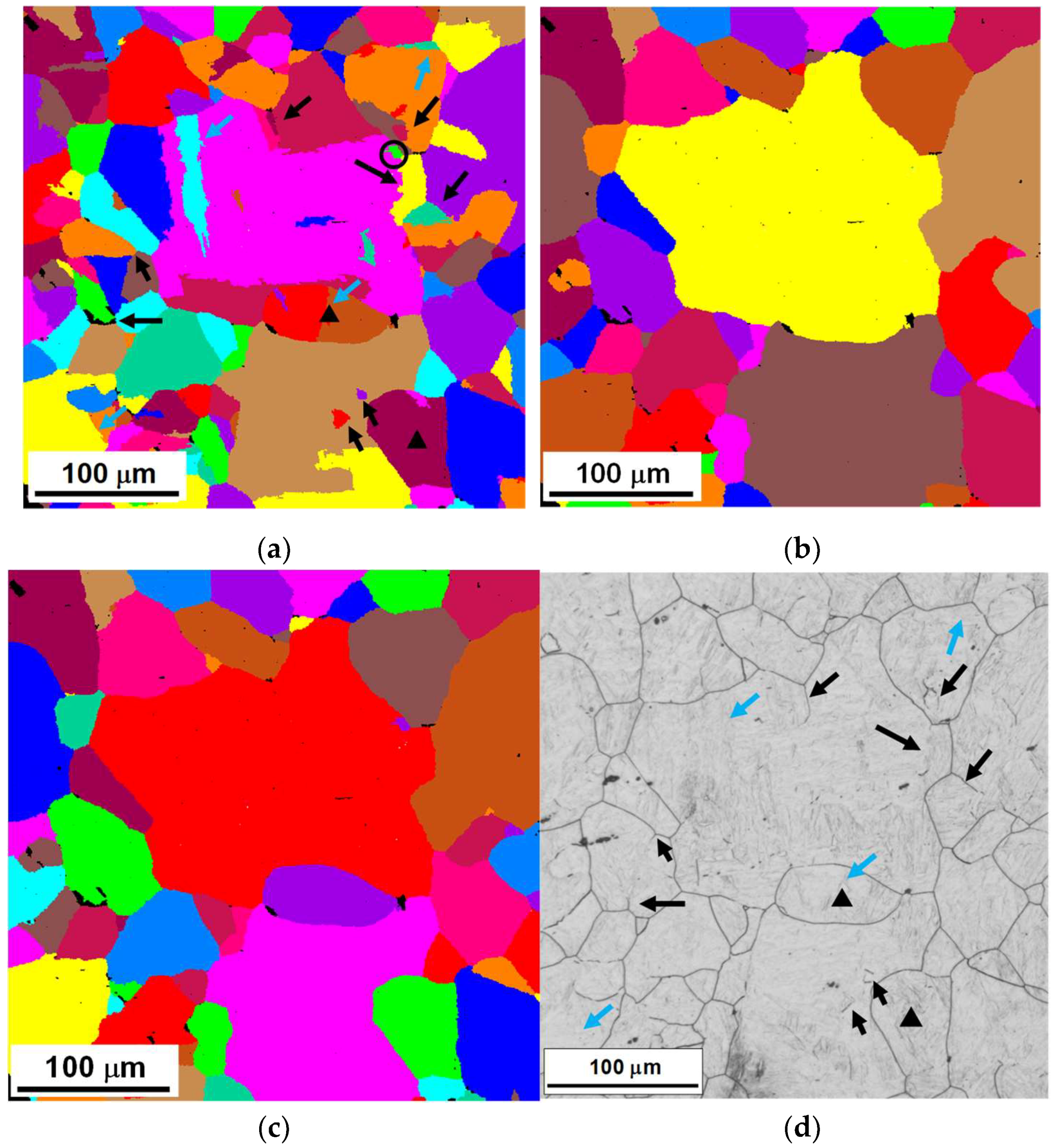
4.1.1. Grain Boundary Character

The reconstructed austenite maps shown above reveal a large number of misoriented areas within the boundaries revealed by the picric acid. Chemically etching the austenite from quenched martensite using picric acid is complex and has been shown to lead to variable results depending on the solvent and wetting agents [7]. In some studies, the susceptibility of grain boundaries to etching has been related to phosphor segregation [8], although the factors resulting in this effect are not clear and other elements may also contribute. As suggested by Bernier et al. [9], highly ordered or coherent grain boundaries are likely to show a low concentration of segregated elements and therefore be the most resistant to etching. In austenite, the most abundant type of special boundaries are ∑3 annealing twins, which can form during recrystallization or grain growth [30] and can therefore be expected to be present in the analyzed microstructures. For the fcc crystal structure, the primary recrystallization twin can be described as a 60° rotation around the <111> crystal axis. However, for a twin to be coherent, a second condition must be fulfilled: the boundary plane must coincide with the twinning plane. This means that the {111} planes on either side of the boundary must be aligned with the boundary plane. Unfortunately, EBSD scans are 2-dimensional, and the plane of the boundary cannot be determined from the crystallographic data [31]. However, several criteria have been proposed to assess the coherence of twins from orientation imaging data. The less restrictive criterion was proposed by Brandon [32] and consists in applying an angular tolerance from the exact CSL (Coincident Site Lattice) misorientation (60° degree rotation around the <111>), such that it can be accommodated by arrays of dislocations. For ∑3 this results in a tolerance angle of 8.66°, although more stringent tolerance angle criteria have been proposed in other works [33]. Another second criterion for checking the coherence of the twin from the scan data is to verify that the {111} twin planes at either side of the boundary are common [34,35]. A third criterion for twin boundary coherence is that the boundary trace and the twin plane traces should coincide [31,34,35,36].

Figure 7a and Figure 8a show the unique grain color maps obtained using a tolerance angle for a grain boundary definition of 10° from the reconstructed maps with a 0.5 μm and 1.5 μm step size, respectively, while Figure 7b,c and Figure 8b,c correspond to the same maps but exclude twins as grain boundaries. In the case of Figure 7b and Figure 8b, the twins were defined as grain boundaries deviated from the exact CSL misorientation by less than 5°. This is equivalent to applying Brandon’s criterion, but using a slightly more restrictive angular deviation, one that is closer to those proposed by others [33]. The same grain tolerance has been employed in other studies to identify coherent twins [34]. In the case of Figure 7c and Figure 8c, as well as the previous criterion, the alignment of {111} planes at either side of the boundary (with a tolerance angle lower than 1°) was imposed for twin boundary classification. To do this, the “Enforce matching between twin planes in grain A and grain B” option included in the twin boundary tab definition in the TSL OIM software [26] was used. As mentioned above, a third check consisting of matching the {111} plane traces and the grain boundary trace could be imposed. Unfortunately, our current version of EBSD analysis software (TSL OIM Analysis 5.31) (EDAX, Mahwah, NJ, USA) does not support the ability to reconstruct boundaries and therefore to perform this type of analysis in the case of square grid scans, so this was not considered. Nevertheless, it must be mentioned that Henrie et al. [34] found that the combination of the misorientation and twin boundary plane alignment criteria was sufficient for verifying the coherence of most twin boundaries.

It can be observed from both figures that the number of detected grains decreases significantly when the twin boundaries are excluded independently of the twin identification criterion used. At first glance, there is much better agreement between the grain boundaries revealed by picric acid etching (Figure 3a–c) and the grain size maps obtained by excluding the twins. It could be argued that the reconstruction procedure leads to the misindexing of some areas as twins, as has been observed in other cases when the Kurjumov-Sachs or the Nishiyama-Wasserman orientation relationships were applied [16]. However, in a previous study carried out with an Fe-30Ni alloy [18], in which the austenite microstructure was available to validate the reconstruction procedure, the ability of the software to reconstruct twin boundaries was verified and fake twinned regions were not observed in the reconstructed austenite microstructures. Miyamoto et al. [16] showed that the frequency of misindexed twins decreases significantly when an orientation relationship with martensite and austenite holding a non-parallel relation between close-packed planes, such as the one applied here, is used instead of the Kurjumov-Sachs or the Nishiyama-Wasserman orientation relationships. The calculated number of variants required for a valid identification ($N_v=2$ [16]) is in fact lower than the more restrictive criterion used in this research, $N_v=4$. Moreover, it can be observed from comparing the picric acid etched microstructures that some of the boundaries which do not close to delineate grains or which are fainter are in very good agreement with boundaries which are present in Figure 7a or Figure 8a but not in Figure 7b,c or Figure 8b,c (see examples marked with the black arrows in Figure 7 and Figure 8). This indicates that there can be a significant number of twins in the austenite microstructure that are not revealed by etching (some examples have been marked with blue arrows in Figure 7a,d) and that cannot therefore be characterized using conventional metallographic techniques.

There is good agreement between the austenite morphology obtained by metallography and the grain maps obtained from the reconstruction results that exclude twin boundaries. However, it is difficult to determine from the maps which of the two twin exclusion criteria is more comparable to the metallographic results. For example, in the case of Figure 7b some of the grains revealed by picric acid etching (Figure 3a) are not present, while these can be detected in Figure 7c (two obvious examples have been marked in Figure 7a with triangles). This indicates that applying the twin plane criterion results in more accurate grain boundary classification in some cases. However, some of the smallest grains present in Figure 7c, such as the grain marked with a circle in Figure 7a, are not revealed in the optical micrographs. Applying a larger tolerance angle for the twin plane criterion (3° instead of 1°) led to the inclusion of the encircled grain as a twinned region inside the larger one, as shown in Figure 7b. However, the same thing happens with the two grains marked by triangles. This shows that selecting a single criterion for an optimum match is difficult. Some uncertainty in the orientations determined from the reconstruction results is to be expected. In addition, the degree of incoherence necessary for the grain boundaries to be susceptible to etching is not known, and neither in fact is the question of whether the segregation of elements to boundaries (which is thought to be the factor enabling metallographic etching) is homogeneous within the sample.

To further confirm the nature of these boundaries as twins, the crystallography of the martensite at either sides of the boundary was in some cases also analyzed. The results are summarized in Figure 9 and Figure 10. In Figure 9a and Figure 10a the selected analysis areas have been marked over the ND IPF maps, and Figure 9b and Figure 10b include the same data corresponding only to the selected zones. A comparison of the ND IPF maps with those in Figure 7 reveals the presence, within these areas, of grain boundaries which have been classified as twins and are not revealed by etching. The {001} pole figures obtained from these areas have been plotted in Figure 9d and Figure 10d, including all the orientation data (points in black). In addition, in the pole figures, data at either sides of the grain boundary have been highlighted either in blue (left side) or in red (right side). To clarify the specific crystallographic data marked in each case, in Figure 9c and Figure 10c the areas selected for the highlighting have been superimposed over the ND IPF maps using the same colors. It is interesting to note that, for both examples, data for each of the boundaries results in clearly differentiated pole figures. Moreover, there is a large similarity between these pole figures and those simulated by Germain et al. for martensite when this is transformed from twinned zones (see Figure 7a in [10]). Only a few crystallographic data deviate in the case of Figure 10d. This further confirms the nature of these grain boundaries as twins.

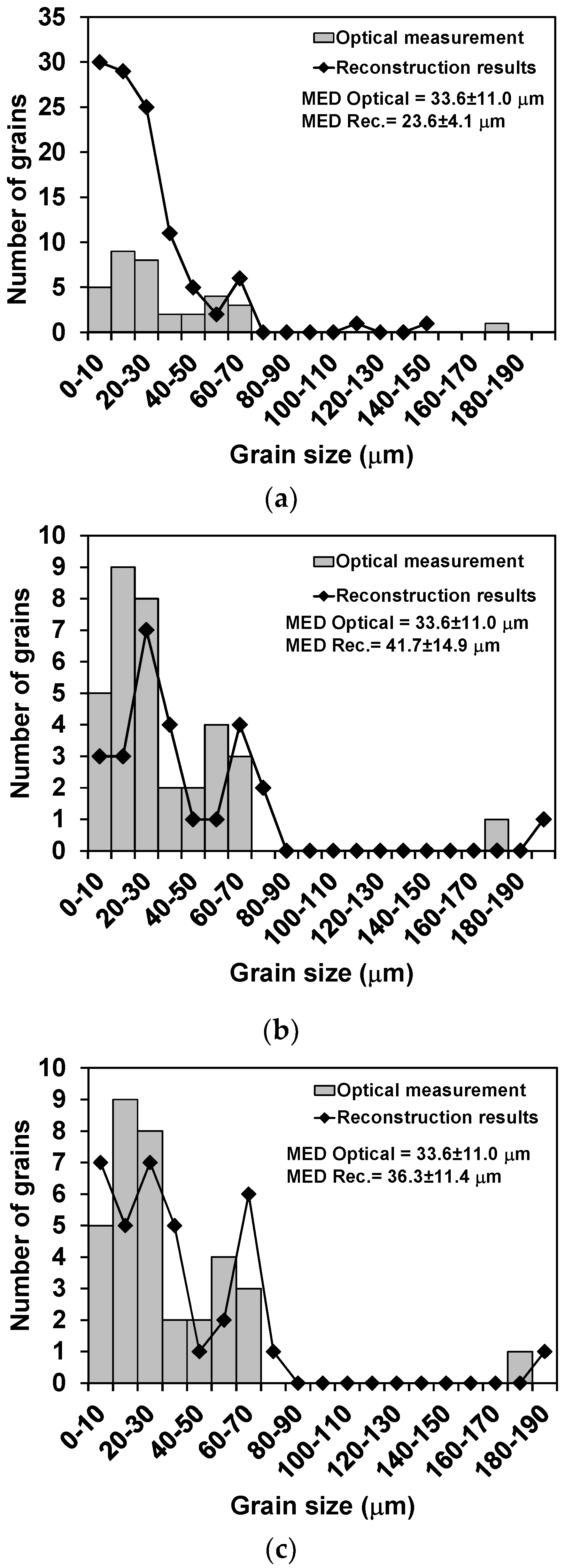
4.1.2. Grain Size Measurements

To obtain a more quantitative assessment, the grain size distributions obtained from the optical micrographs and the EBSD reconstructed maps for the three different scans are compared in Figure 11, Figure 12 and Figure 13. The average MED values obtained in all cases are also included in the figures. In the reconstruction grain size measurements, a minimum grain size of 4 μm was considered, which corresponds approximately to the smallest grain size measured by optical microscopy, and border grains were excluded as in the case of conventional metallography. It can be observed that in the figures the grain size measurements have been compared as a function of the absolute number of grains. Although this is not a conventional method for grain size distribution representation, the fact that the distributions compared in each of the graphs were obtained from approximately the same specimen area must be taken into account, and that this is therefore preferred in this case since, in addition to comparing the shape of the distributions, it is possible to compare the number of grains detected in each of the measurements.

It can be observed from Figure 11a, Figure 12a and Figure 13a that, as expected from the above results, quantifying the grain size from the reconstructed austenite maps without excluding twins results in a significantly larger number of measured grains compared to the metallographic data and also results in smaller average grain sizes (23.6, 36.4 and 37.2 μm versus 33.6, 54.6 and 46.7 μm for 0.5, 1 and 1.5 μm step size scans, respectively). In contrast, when only one misorientation criterion is applied to exclude twin boundaries (Figure 11b, Figure 12b and Figure 13b), the number of grains measured from the reconstruction tends to be lower, and as a consequence, the average grain sizes are coarser than those measured by metallography (41.7, 65.6 and 55.9 μm for 0.5, 1 and 1.5 μm step sizes). This occurs especially for the 1.5 μm step size scan (Figure 13b). On the other hand, the three scans show excellent agreement for the average grain size values when the misorientation and twin boundary plane criteria are applied (36.3, 52.3 and 48.9 μm for 0.5, 1 and 1.5 μm step sizes, respectively). Regarding the grain size distributions, in Figure 11c the fit can be considered reasonable. A good correlation is also found in Figure 12c and Figure 13c, although slightly opposite trends can be observed. In the case of the 1 μm step size scan (Figure 12c), the number of grains measured from the reconstruction tends to be larger than that from the metallographic measurement, especially in the range of the smallest sizes, while in the 1.5 μm step size scan (Figure 13c) the opposite occurs. It must be mentioned that the differences are not large and are difficult to evaluate. However, in the case of the 1 μm step size, comparing the sketch used for the metallographic measurement to the reconstructed grain map revealed the presence of some small grains in the reconstruction which were only partially revealed by chemical etching. This can explain the larger number of small grains present in the reconstructed austenite grain size distribution. On the other hand, in the case of the 1.5 μm step size, some of the smallest grains were not reconstructed. This step size may be too large to resolve the minimum number of required variants for grain reconstruction in the case of the smallest grains present in the microstructure. Although this may be optimized by varying the parameter of the reconstruction [18], it must be mentioned that this happened in very few examples, as can be seen from the visual comparison of Figure 4c and Figure 8. Paradoxically in this case, since the etching quality was better (Figure 3c), it resulted in a higher number of “questionable” grain boundaries included in the sketch. This clearly reflects the dependence of the metallographic results on the etching quality.

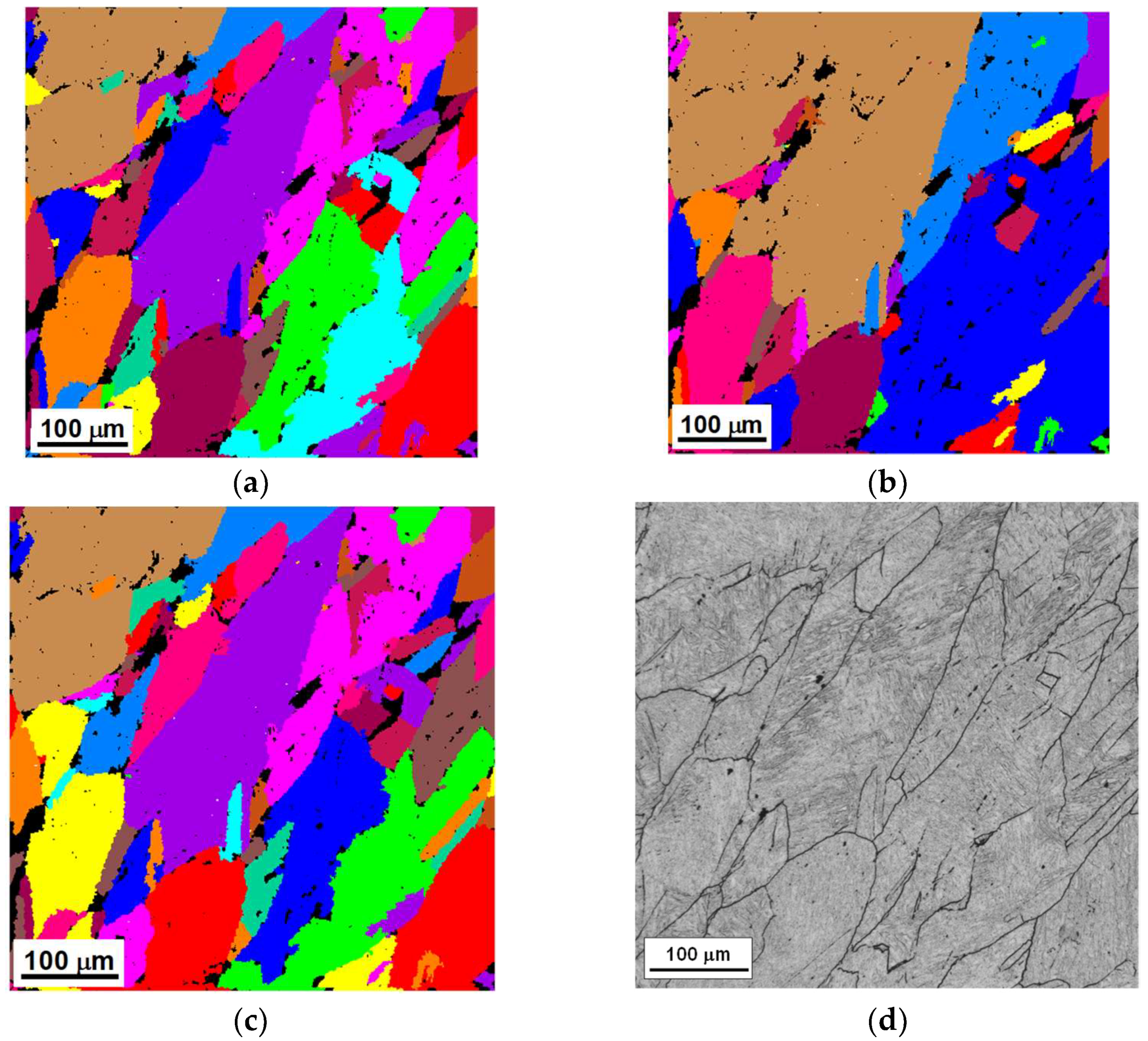
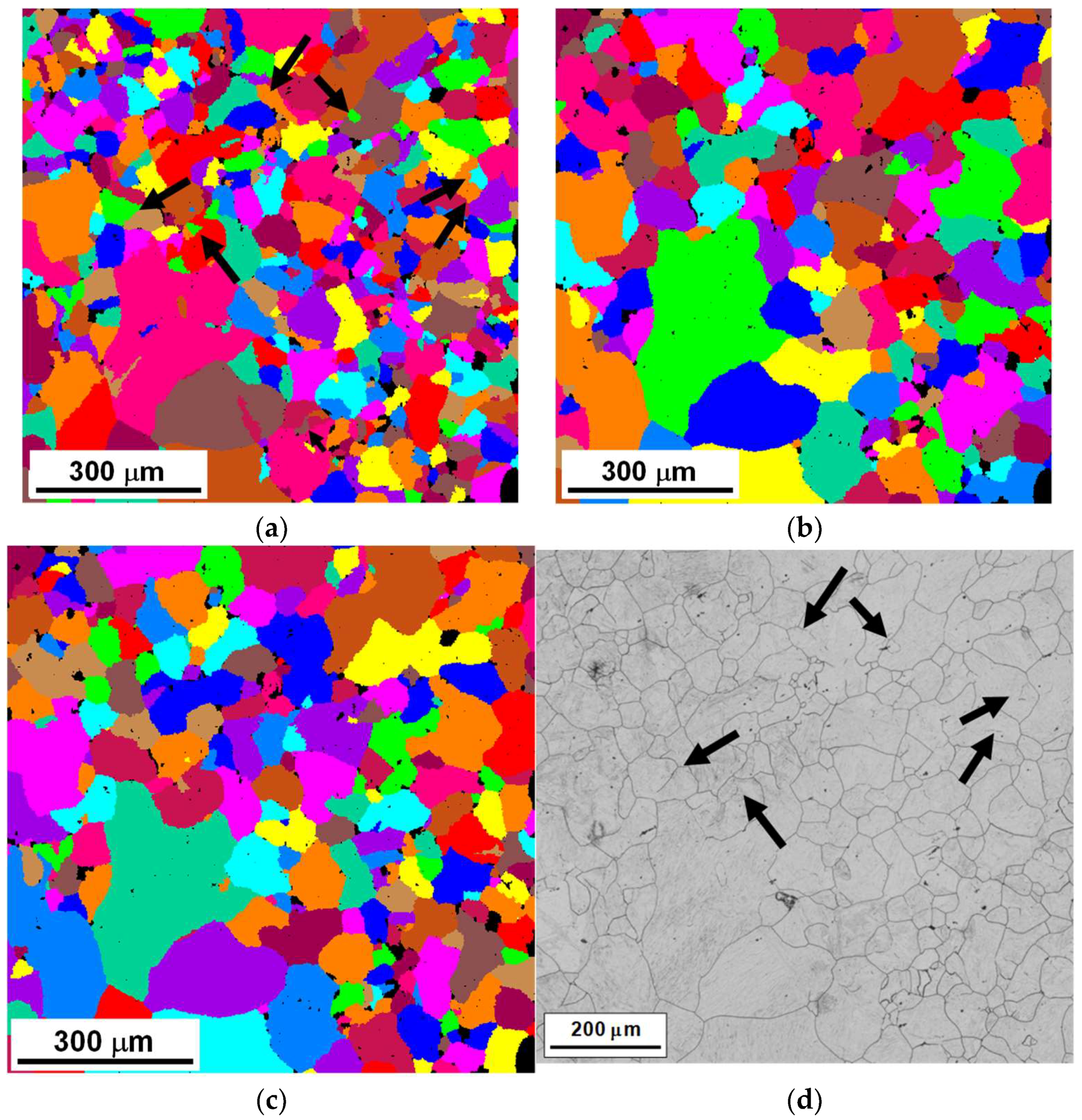
4.2. Deformed Microstructure

In addition to determining the grain size in recrystallized samples, there is also an interest in characterizing deformed austenite microstructures. As shown in Figure 6d, for the deformed microstructure studied in this article, applying the reconstruction procedure resulted in a large reconstructed area fraction of 95%. Although, in this case, the grain size measurement was not conducted due to being more complex because of austenite pancaking, Figure 14 includes the unique grain color maps obtained from the reconstruction using a tolerance angle of 10° and applying the same criteria as above for grain boundary definition. At first glance, a good correlation is also observed between the reconstructed grain maps and the metallographic results. However, it is interesting to note that, in contrast with the results obtained in the recrystallized microstructure, the best visual match with the chemically etched microstructure is obtained for Figure 14a (twin boundaries not excluded) and Figure 14c (twin boundaries defined using misorientation and twin plane criteria). On the other hand, in Figure 14b (twin boundaries defined using only the misorientation criterion) some of the boundaries revealed by etching are not present, while coarser austenite units which are not observed in the optical micrograph are present. In the case of the recrystallized microstructure studied in the previous sections, the differences between the maps obtained when applying either of the two criteria used for excluding twins (misorientation or the misorientation and twin boundary criteria) were small compared with those obtained when considering all high angle boundaries as grain boundaries. However, in this deformed microstructure, the reconstructed austenite grain maps tend to be more similar in the case of Figure 14a,c. In this sample, applying the roughing passes at high temperature is expected to lead to successive cycles of recrystallization and grain growth, which are likely to result in the generation of a significant amount of coherent twins [30], such as the ones found in the recrystallized microstructure analyzed in the previous sections. In this type of recrystallized microstructure, coherent twin boundaries were in most cases correctly detected using either of the considered criteria. However, in this sample, during finishing the microstructure was deformed below the non-recrystallization temperature. This is likely to result in the rotation of the crystals at both sides of the twin boundaries. In principle, this should result in a failure of the {111} plane coincidence criterion. It is interesting to note that, in good agreement with this, most of the boundaries present in Figure 14c and not in Figure 14b are actually revealed using Bechet-Beaujard etching [6], which suggests that during the deformation, loss of twin boundary coherence is actually taking place. The progressive loss of twin boundary coherence during deformation has been observed experimentally in Fe-30Ni model austenitic steels analyzed by EBSD [37]. On the other hand, the less stringent application of the misorientation criterion only (Figure 14b) seems to lead to incorrect grain boundary classification for this deformed microstructure.

5. Conclusions

-

The austenite morphology and grain size measurements obtained by applying conventional metallographic techniques to reveal the previous austenite grain boundaries from quenched martensite (Bechet-Beaujard etching) were compared with the results of a reconstruction procedure applied to orientation imaging data collected from the same martensitic specimens, quenched from both recrystallized and deformed austenite. The austenite morphology revealed by both methods showed a good correspondence in the two microstructures investigated, although their comparability strongly depends on the criteria used for grain boundary definition in the reconstructed austenite maps.

-

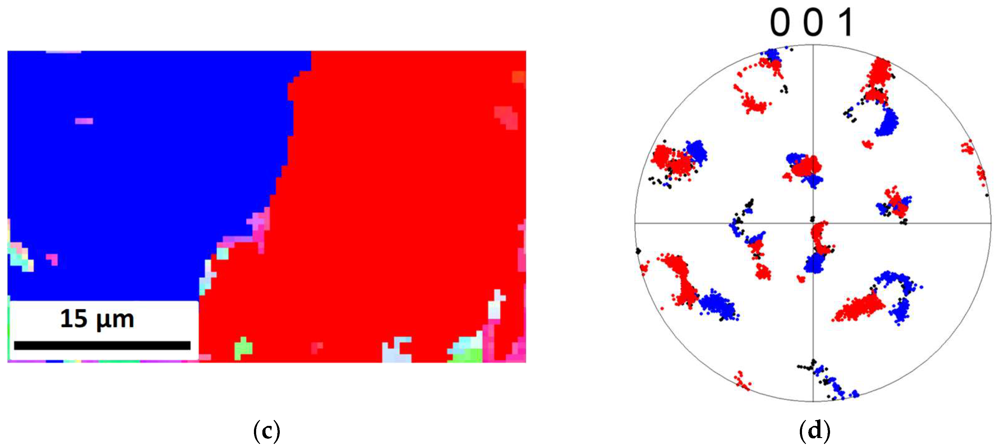
In the case of the recrystallized microstructure, the reconstruction procedure showed the presence of a large number of coherent twin boundaries in the microstructure that were not revealed by chemical etching. Although the coherence of the twin boundaries cannot be completely assessed from the crystallographic recovered data, in this microstructure the application of misorientation or misorientation plus twin boundary plane criteria for twin boundary exclusion led to a good correspondence between the morphology revealed by metallographic methods and the reconstruction results.

-

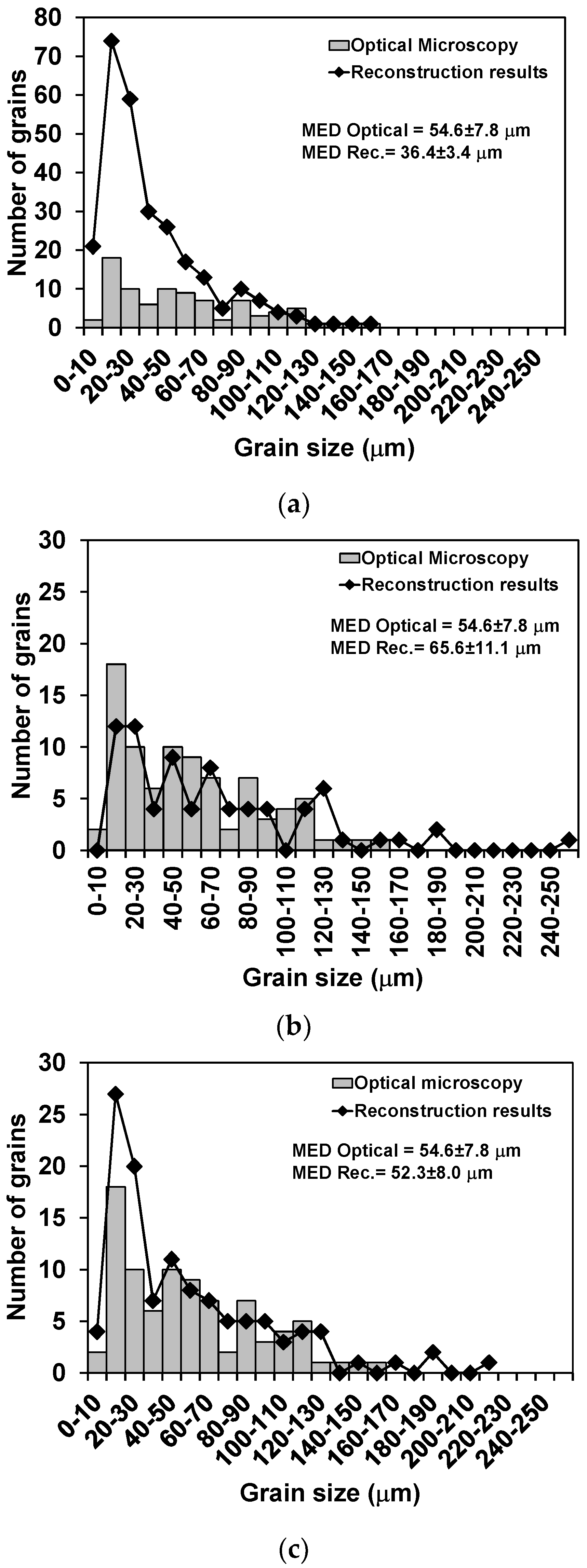
A very good correlation between the average grain size and the size distribution determined by conventional metallography and the reconstruction method was observed when the grain boundary misorientation plus twin boundary coincidence criteria were used for twin boundary exclusion from the reconstruction measurements. On the other hand, considering all the reconstructed boundaries resulted in a large overestimation of the number of grains present in the microstructure compared to the metallographic results, as well as in an underestimation of the average grain size. Using only the misorientation criteria led to larger grain size than the optical MED. The effect on the results of varying the step size from 0.5 to 1.5 μm for EBSD acquisition was small, showing the ability of the reconstruction method to provide quantitative measurements in areas representative of the analyzed austenite microstructure.

-

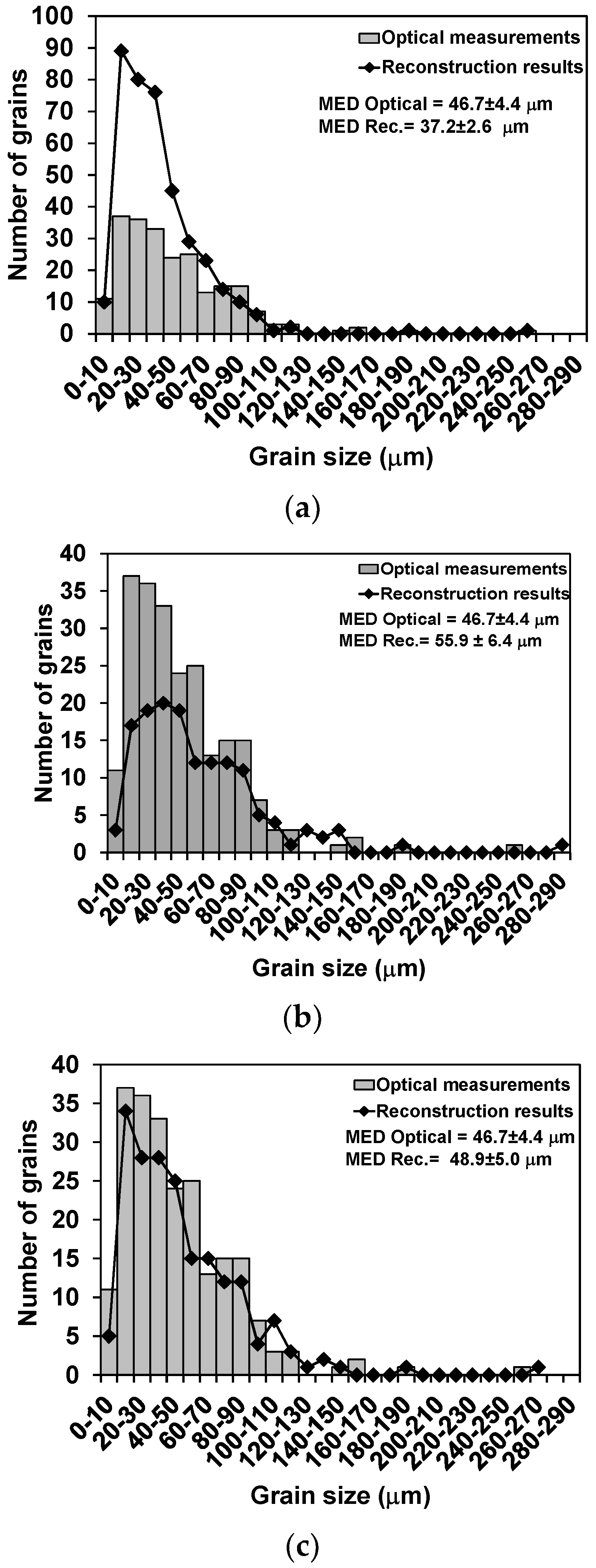
In the microstructure quenched after applying several roughing and finishing passes, a good correspondence between the conventional metallography austenite morphology and the reconstruction results was also obtained when the misorientation and twin boundary criteria were used for twin exclusion from the grain size maps. However, in this case, the results were also comparable to considering all high angle grain boundaries for grain definition. This can be attributed to the loss in twin boundary coherence during the finishing deformation passes. However, the less stringent application of the misorientation criterion only led to an incorrect grain boundary classification and in some cases to the reunification of some of the deformed twinned regions which had lost coherence.

References

1. Hodgson, P.D.; Gibb, R.K. Mathematical model to predict the mechanical properties of hot rolled C-Mn and Microalloyed steels. ISIJ Int. 1992, 32, 1329–1338. [Google Scholar] [CrossRef]
2. Bengochea, R.; López, B.; Gutiérrez, I. Influence of the prior austenite microstructure on the transformation products obtained for C-Mn-Nb steels after continuous cooling. ISIJ Int. 1999, 39, 583–591. [Google Scholar] [CrossRef]
3. Ray, R.K.; Jonas, J.J.; Butron-Guillen, M.P.; Savoie, J. Transformation textures in steels. ISIJ Int. 1994, 34, 927–942. [Google Scholar] [CrossRef]
4. Andrade, H.L.; Akben, M.G.; Jonas, J.J. Effect of molybdenum, niobioum, and vanadium on static recovery and recrystallisation and on solute strengthening in microalloyed steels. Metall. Mater. Trans. A 1983, 14, 1967–1977. [Google Scholar] [CrossRef]
5. Fernández, A.I.; López, B.; Rodríguez-Ibabe, J.M. Relationship between the austenite recrystallised fraction and the softening measured from the interrupted torsion test technique. Scr. Mater. 1999, 40, 543–549. [Google Scholar] [CrossRef]
6. Bechet, S.; Beaujard, L. New Reagent for the micrographical demonstration of the austenite grain of hardened or hardened-tempered steels. Rev. Met. 1955, 52, 830–836. [Google Scholar] [CrossRef]
7. Barraclough, D.R. Etching of prior austenite grain boundaries in martensite. Metallography 1973, 6, 465–472. [Google Scholar] [CrossRef]
8. Ücisik, A.H.; McMahon, C.J.; Feng, H.C. The influence of intercritical heat treatment on the temper embrittlement of a P-doped Ni-Cr steel. Metall. Trans. 1978, 9A, 321–329. [Google Scholar] [CrossRef]
9. Bernier, N.; Bracke, L.; Malet, L.; Godet, S. An alternative to the crystallographic reconstruction of austenite in steels. Mater. Charact. 2014, 89, 23–32. [Google Scholar] [CrossRef]
10. Germain, L.; Gey, N.; Mercier, R.; Blaineau, P.; Humbert, M. An advanced approach to reconstructing parent orientation maps in the case of approximate orientation relations: Application to steels. Acta Mater. 2012, 60, 4551–4562. [Google Scholar] [CrossRef]
11. Humbert, M.; Wagner, F.; Moustahfid, H.; Esling, C. Determination of the orientation of a parent β grain from the orientations of the inherited α plates in the phase transformation from body-centred cubic to hexagonal close packed. J. Appl. Cryst. 1995, 28, 571–576. [Google Scholar] [CrossRef]
12. Humbert, M.; Gey, N. The calculation of a parent orientation from inherited variants for approximate (b.c.c.-h.c.p.) orientation relations. J. Appl. Cryst. 2002, 35, 401–405. [Google Scholar] [CrossRef]
13. Gey, N.; Humbert, M. Specific analysis of EBSD data to study the texture inheritance due to the β → α phase transformation. J. Mater. Sci. 2003, 38, 1289–1294. [Google Scholar] [CrossRef]
14. Cayron, C.; Artaud, B.; Briottet, L. Reconstruction of parent grains from EBSD data. Mater. Charact. 2006, 57, 386–401. [Google Scholar] [CrossRef]
15. Tari, V.; Rollett, A.D.; Beladi, H. Back calculation of parent austenite orientation using a clustering approach. J. Appl. Cryst. 2013, 46, 210–215. [Google Scholar] [CrossRef]
16. Miyamoto, G.; Iwata, N.; Takayama, N.; Furuhara, T. Mapping the parent austenite orientation reconstructed from the orientation of martensite by EBSD and its application to ausformed martensite. Acta Mater. 2010, 58, 6393–6403. [Google Scholar] [CrossRef]
17. Miyamoto, G.; Iwata, N.; Takayama, N.; Furuhara, T. Reconstruction of parent austenite grain structure based on crystal orientation map of bainite with and without ausforming. ISIJ Int. 2011, 51, 1174–1178. [Google Scholar] [CrossRef]
18. Sanz, L.; Pereda, B.; López, B. Validation and analysis of the parameters for reconstructing the austenite phase from martensite electron backscatter diffraction data. Metall. Mater. Trans. A 2017, 48, 5258–5272. [Google Scholar] [CrossRef]
19. Pereda, B.; Aretxabaleta, Z.; López, B. Softening kinetics in high Al and high Al-Nb-microalloyed steels. J. Mater. Eng. Perform. 2015, 24, 1279–1293. [Google Scholar] [CrossRef]
20. Pereda, B.; Fernandez, A.I.; López, B.; Rodríguez-Ibabe, J.M. Effect of Mo on dynamic recrystallization behavior of Nb-Mo microalloyed steels. ISIJ Int. 2007, 47, 860–868. [Google Scholar] [CrossRef]
21. Gomez, M.; Rancel, L.; Medina, S.F. Assessment of austenite static recrystallization and grain size evolution during multi-pass hot rolling of a niobium-microalloyed steel. Met. Mater. Int. 2009, 15, 689–699. [Google Scholar] [CrossRef] [Green Version]
22. Weyand, S.; Britz, D.; Mücklich, F. Investigation of austenite evolution in low-carbon steel by combining EBSD data. Mater. Perform. Charact. 2015, 4, 322–340. [Google Scholar]
23. Aretxabaleta, Z.; Pereda, B.; López, B. Multipass hot deformation behaviour of high Al and Al-Nb steels. Mater. Sci. Eng. 2014, 600, 37–46. [Google Scholar] [CrossRef]
24. Aretxabaleta, Z.; Pereda, B.; López, B. Analysis of the effect of Al on the static softening kinetics of C-Mn steels using a physically based model. Metall. Mater. Trans. A 2014, 45, 934–947. [Google Scholar] [CrossRef]
25. Development of Microstructure-Based Tools for Alloy and Rolling Process Design (Microtools); Final Report; Publications Office of the European Union: Luxembourg, 2013; ISBN 978-92-79-33613-3.
26. TSL OIM Analysis 5.31, Package 7000; EDAX: Mahwah, NJ, USA, 2007.
27. The GIMP Team. GIMP 2.8.14. Available online: www.gimp.org (accessed on 5 April 2018).
28. LAS v4.5, Build 418; Leica Microsystems: Wetzlar, Germany, 2016.
29. MATLAB, Release 2013b; The MathWorks, Inc.: Natick, MA, USA, 2013.
30. Jin, Y.; Bernacki, M.; Rohrer, G.S.; Rollett, A.D.; Lin, B.; Bozzolo, N. Formation of annealing twins during recrystallization and grain growth in 304L austenitic stainless steel. Mater. Sci. Forum 2013, 753, 113–116. [Google Scholar] [CrossRef]
31. Wright, S.I.; Larsen, R.J. Extracting twins from orientation imaging microscopy scan data. J. Microsc. 2002, 205, 245–252. [Google Scholar] [CrossRef] [PubMed]
32. Brandon, D.G. The structure of high-angle grain boundaries. Acta Metall. 1966, 14, 1479–1484. [Google Scholar] [CrossRef]
33. Palumbo, G.; Aust, K.T.; Lehockey, E.M.; Erb, U. On a more restrictive geometric criterion for “special” CSL grain boundaries. Scr. Mater. 1998, 38, 1685–1690. [Google Scholar] [CrossRef]
34. Henrie, B.L.; Mason, T.A.; Hansen, B.L. A semiautomated electron backscatter diffraction technique for extracting reliable twin statistics. Metall. Mater. Trans. A 2004, 35, 3745–3751. [Google Scholar] [CrossRef]
35. Mason, T.A.; Bingert, J.F.; Kaschner, G.C.; Wright, S.I.; Larsen, R.J. Advances in deformation twin characterization using electron backscattered diffraction data. Metall. Mater. Trans. A 2002, 33, 949–954. [Google Scholar] [CrossRef]
36. Randle, V. A methodology for grain boundary plane assessment by single-section trace analysis. Scr. Mater. 2001, 44, 2789–2794. [Google Scholar] [CrossRef]
37. Poddar, D.; Cizek, P.; Beladi, H.; Hodgson, P.D. Orientation dependence of the deformation microstructure in a Fe-30Ni-Nb model austenitic steel subjected to hot uniaxial compression. Scr. Mater. 2001, 44, 2789–2794. [Google Scholar] [CrossRef]
Figure 1. Experimental setup for the EBSD (Electron Back-Scatter Diffraction) scan acquisition and area of analysis in the torsion specimens.
Metals 08 00294 g001
Figure 2. IPF (Inverse pole figure) ND (Normal Direction) maps obtained from the martensitic sample quenched from recrystallized austenite using different step sizes and scan areas. (a) Step size = 0.5 μm, 350 × 350 μm2; (b) step size = 1 μm, 800 × 700 μm2; and (c) step size = 1.5 μm, 900 × 900 μm2.
Metals 08 00294 g002
Figure 3. Optical micrographs of the martensitic sample quenched from recrystallized austenite revealed by Bechet-Beaujard etching [6] in the areas corresponding to the EBSD scans of Figure 2. (a) 350 × 350 μm2; (b) 800 × 700 μm2; and (c) 900 × 900 μm2. In (a,b), the arrows represent boundaries which show weaker contrast and/or which do not close to define grains.
Metals 08 00294 g003
Figure 4. Grain boundary sketches used for optical grain size determinations obtained from micrographs in Figure 3. (a) 350 × 350 μm2, MED (mean equivalent diameter) = 33.6 ± 11.0 μm; (b) 800 × 700 μm2, MED = 54.6 ± 7.8 μm; and (c) 900 × 900 μm2, MED = 46.7 ± 4.4 μm.
Metals 08 00294 g004aMetals 08 00294 g004b
Figure 5. (a) IPF (Inverse pole figure) ND map obtained from the martensitic sample quenched from deformed austenite; and (b) corresponding optical micrograph taken after Bechet-Beaujard etching from the martensitic sample (Step size = 1 μm, 500 × 500 μm2).
Metals 08 00294 g005
Figure 6. IPF (Inverse pole figure) austenite ND orientation maps obtained from the reconstruction results applied to the martensitic scan data. Black areas represent non-reconstructed regions. (a) Recrystallized microstructure, step size = 0.5 μm, 99.5% reconstructed; (b) recrystallized microstructure, step size = 1 μm, 99.5% reconstructed; (c) recrystallized microstructure, step size = 1.5 μm, 97.8% reconstructed; and (d) deformed microstructure, step size = 1 μm, 95.1% reconstructed.
Metals 08 00294 g006aMetals 08 00294 g006b
Figure 7. Unique grain color maps obtained for the austenite phase from the results of the reconstruction applied to the martensitic scan data in Figure 2a (Step size = 0.5 μm) using a tolerance angle for a grain boundary definition of 10° and different criteria for twin boundary exclusion: (a) All high angle grain (>10°) boundaries considered; (b) twins excluded (misorientation criterion (5° tolerance)); (c) twins excluded (misorientation criterion (5° tolerance) + {111} plane coincidence criterion (1° tolerance angle)) and (d) optical micrograph. Black areas correspond to non-reconstructed regions. In (a,d) black arrows mark boundaries which are present in (a) but not in (b) and/or (c), and which appear faintly or do not close to define grains in the optical micrograph in (d); blue arrows mark twins which are not revealed in the optical micrograph in (d); triangles mark grains that can be observed in (c,d) but not in (b).
Metals 08 00294 g007
Figure 8. Unique grain color maps obtained for the austenite phase from the results of the reconstruction applied to the martensitic scan data from Figure 2c (Step size = 1.5 μm) using a tolerance angle for a grain boundary definition of 10° and different criteria for twin boundary exclusion: (a) All high angle grain (>10°) boundaries considered; (b) twins excluded (misorientation criterion (5° tolerance)); (c) twins excluded (misorientation criterion (5° tolerance) + {111} plane coincidence criterion (1° tolerance angle)); (d) optical micrograph. Black areas correspond to non-reconstructed regions. In (a,d) arrows mark boundaries which are present in (a) but not in (b) and/or (c), and which appear faintly or do not close to define grains in the optical micrograph in (d).
Metals 08 00294 g008
Figure 9. (a) IPF (Inverse pole figure) ND orientation map from martensite marking the analysis area; (b) enlarged martensite IPF ND map of the analysis area; (c) martensite IPF ND map of the same area with red and blue colors superimposed to mark highlighted points in (d); (d) pole figure of the crystallographic data in (b) with points corresponding to areas in (c) highlighted using the same colors.
Metals 08 00294 g009
Figure 10. (a) IPF (Inverse pole figure) ND orientation map from martensite marking the analysis area; (b) enlarged martensite IPF ND map of the analysis area; (c) martensite IPF ND map of the same area with red and blue colors superimposed to mark highlighted points in (d); (d) pole figure of the crystallographic data in (b) with points corresponding to areas in (c) highlighted using the same colors.
Metals 08 00294 g010aMetals 08 00294 g010b
Figure 11. Comparison of the MED (Mean Equivalent Diameter) measurements obtained from conventional metallography and the reconstruction procedure for the 0.5 μm step size scan using different criteria for twin boundary definition (4 μm minimum grain size): (a) All high angle (>10°) grain boundaries considered; (b) twins excluded (misorientation criterion (5° tolerance)); and (c) twins excluded (misorientation criterion (5° tolerance) + {111} plane coincidence criterion (1° tolerance angle)).
Metals 08 00294 g011
Figure 12. Comparison of the MED measurements obtained from conventional metallography and the reconstruction procedure for the 1 μm step size scan using different criteria for twin boundary definition (4 μm minimum grain size): (a) All high angle (>10°) grain boundaries considered; (b) twins excluded (misorientation criterion (5° tolerance)); and (c) twins excluded (misorientation criterion (5° tolerance) + {111} plane coincidence criterion (1° tolerance angle).
Metals 08 00294 g012
Figure 13. Comparison of the MED measurements obtained from conventional metallography and the reconstruction procedure for the 1.5 μm step size scan using different criteria for twin boundary definition (4 μm minimum grain size): (a) All high angle (>10°) grain boundaries considered; (b) twins excluded (misorientation criterion (5° tolerance)); and (c) twins excluded (misorientation criterion (5° tolerance) + {111} plane coincidence criterion (1° tolerance angle)).
Metals 08 00294 g013
Figure 14. Unique grain colormaps obtained from the deformed austenite microstructures applying the reconstruction procedure to the martensitic scan in Figure 5a using a tolerance angle for grain boundary definition of 10° and different criteria for twin boundary exclusion: (a) All the high angle grain boundaries considered; (b) twins excluded (misorientation criterion (5° tolerance)); (c) twins excluded (misorientation criterion (5° tolerance) + {111} plane coincidence criterion (1° tolerance angle)) and (d) optical micrograph. Black areas correspond to non-reconstructed regions.
Metals 08 00294 g014