A New Cumulative Fatigue Damage Rule Based on Dynamic Residual S-N Curve and Material Memory Concept

1
School of Mechanical and Electrical Engineering, University of Electronic Science and Technology of China, Chengdu 611731, China
2
Center for System Reliability and Safety, University of Electronic Science and Technology of China, Chengdu 611731, China
*
Author to whom correspondence should be addressed.
Metals 2018, 8(6), 456; https://doi.org/10.3390/met8060456
Submission received: 23 May 2018
/
Revised: 7 June 2018
/
Accepted: 7 June 2018
/
Published: 14 June 2018
Abstract
:This paper introduces a new phenomenological cumulative damage rule to predict damage and fatigue life under variable amplitude loading. The rule combines a residual S-N curve approach and a material memory concept to describe the damage accumulation behavior. The residual S-N curve slope is regarded as a variable with respect to the loading history. The change in slope is then used as a damage measure and quantified by a material memory degeneration parameter. This model improves the traditional linear damage rule by taking the load-level dependence and loading sequence effect into account, which still preserves its superiority. A series of non-uniform fatigue loading protocols are used to demonstrate the effectiveness of the proposed model. The prediction results using the proposed model are more accurate than those using three popular damage models. Moreover, several common characteristics and fundamental properties of the chosen fatigue models are extracted and discussed.
1. Introduction
In practical engineering, most structural components and mechanical parts in service usually endure the cyclic fluctuating loads with varying intensity. Fatigue is the major cause of the catastrophic failures of these elements or parts. Fatigue failure invariably occurs in the localized weak areas of the material and permanently deteriorates its performance and safe usage. The concept of damage is typically assigned to characterize such a failure process and also plays a fundamental role in fatigue life prediction [1,2,3,4,5]. In spite of extensive investigations to address fatigue theories, the problem of assessing the extent of fatigue damage and then predicting fatigue life still remains a major challenge in fatigue resistant design. Therefore, a reliable cumulative damage rule is strongly expected in structural integrity, reliability-based design, and safety assessments [6]. It should contribute to the increased prediction accuracy, and especially, to obtain maintenance strategies for replacing the damaged elements or parts before failure.
Essentially, fatigue damage mainly includes the process of crack initiation and crack propagation involving various micro-scale behaviors, such as surface extrusion-intrusion, dislocations, plastic slip bands, vacancies, and crack coalescence [7,8]. Although great advancements have been made in the micro-physical mechanisms of fatigue failure, it is not surprising that such analytical theories are relatively complicated and difficult to implement in engineering. In contrast, phenomenological theories [9,10,11,12,13,14] are still the main approaches for fatigue analysis, where simple fatigue formulas that can be identified directly from experiments are preferred. In cases of uniform fatigue loading, some phenomenological formulas are representative and constitute the generic fatigue rules available for many different materials, such as Basquin’s law (stress-life), Manson-Coffin’s law (strain-life), Goodman’s law (mean stress correction), and Paris’ law (crack propagation rate).
However, the fatigue modeling under non-uniform cyclic loading becomes much more intractable due to the complexity of loading histories. In such a fatigue loading, assessment of the damage and fatigue life often relies on cumulative damage theories, including various linear and non-linear hypotheses. A comprehensive overview of cumulative damage and life predictive models has been achieved by Fatemi and Yang [15] and Schijve [16]. The Palmgren-Miner’s hypothesis [17] is acknowledged as a pioneering research on the linear damage rule (LDR) as well as a unified methodology to address fatigue issues under arbitrary non-uniform loading protocols, in spite of limited physical insights and non-conservative predictions. Many researchers suggested that the prediction error of LDR is not necessarily responsible for the linear summation form but mainly responsible for the lack of load-level dependence and loading sequence effects [15,18,19]. Despite the major deficiencies, LDR is still dominantly used in practical engineering design, because the linear summation form can significantly reduce the calculation effort. In order to improve the LDR, a considerable number of non-linear hypotheses [20,21,22,23,24] are proposed to explain the loading sequence observed in the experiments, yet most of them substantially need more parameters to calibrate and are often computationally expensive, especially for multi-stage block loadings when compared with the LDR. The main advantages of LDR lie in its conceptual simplicity, in following a simple linear summation of damage that is inexpensive both computationally and experimentally, and particularly in a small amount of data necessary from the Basquin’s law (S-N curve).
In recent years, fatigue damage modeling in terms of the S-N curve approach has been reported quite intensively and received increasing attention in fatigue life prediction. Corten and Dolan [25] and Freudenthal and Heller [26] put forward a clockwise rotation method of the S-N curve to account for the load interaction effects. Subramanyan [27] introduced an isodamage line to present the damage accumulation process and all of the damage lines were assumed to converge into the knee point of the S-N curve around the endurance limit. Hashin and Rotem [28] extended Subramanyan’s hypothesis and presented a discussion of damage curve families that could pass through either static ultimate or endurance point. Leipholz [29] demonstrated an analytical life-reducing approach to obtain a modified S-N curve, which intersects the original curve at a higher stress level and deviates from it at lower ones. Liu and Mahadevan [19] developed a non-linear cumulative damage model based on the LDR theory, together with a stochastic S-N curve technique, to predict the probabilistic fatigue life of metallic materials under both constant and variable loadings. Lately, Aghoury and Galal [30] proposed a stress-life damage accumulation model by using a concept of virtual target life curve (VTLC) derived from the conventional S-N curve. In this model, fatigue damage is defined as the accumulated loss of the expected life in VTLC, and the loading amplitudes and overloading effects can be captured. Kwofie and Rahbar [31] pointed out that the fatigue failure process was probably dominated by the fatigue driving stress in materials, while also formulating a simple cumulative damage rule using the regular S-N curve. Peng et al. [32] subsequently improved the theory with the strain energy parameter, resulting in more accurate calculations. Several researchers [33,34,35,36,37] suggested a new framework for the damaged stress models connected to the S-N curve to address various fatigue programs, including variable, random, uniaxial, and multiaxial loadings. As stated above, the basic idea of these modeling approaches is to alleviate the effects caused by shortcomings of LDR by considering additional damaging effects responsible for the loading histories. However, most of them are based on the non-linear damage theories, which may cause a large amount of calculation [38,39]. The cumulative damage models are mainly derived from the transformation of the conventional S-N curve that is only suitable for the virgin material without initial damage. Moreover, from the phenomenological point of view, the fatigue damage accumulation is a direct result of irreversible degradation of material properties, whereas the existing models fail to characterize the degradation mechanisms on damage accumulation.
In this paper, a phenomenological damage accumulation model for predicting damage and fatigue life under variable amplitude loading is proposed, which incorporates a residual S-N curve approach and a material memory concept [40]. The residual S-N curve is used to describe the stress-life relation of the damaged material and its slope is considered as a variable with respect to the loading history. Fatigue damage is measured by assessing the change in slope or slope ratio. Then, the material memory concept is introduced to present the material degradation behavior and quantify the slope ratio when accumulating fatigue damage. The proposed model aims to improve the performance of the LDR to make it load-level dependent while still preserving the superiority. A series of experimental data in the literature are used to verify the effectiveness of the model, which covers several metallic materials under non-uniform fatigue loading protocols (two-stage and multi-stage). Moreover, three commonly used cumulative damage rules are chosen for the model comparisons.
2. Formulation of the Proposed Model and Commonly Used Cumulative Damage Rules
2.1. Proposed Model
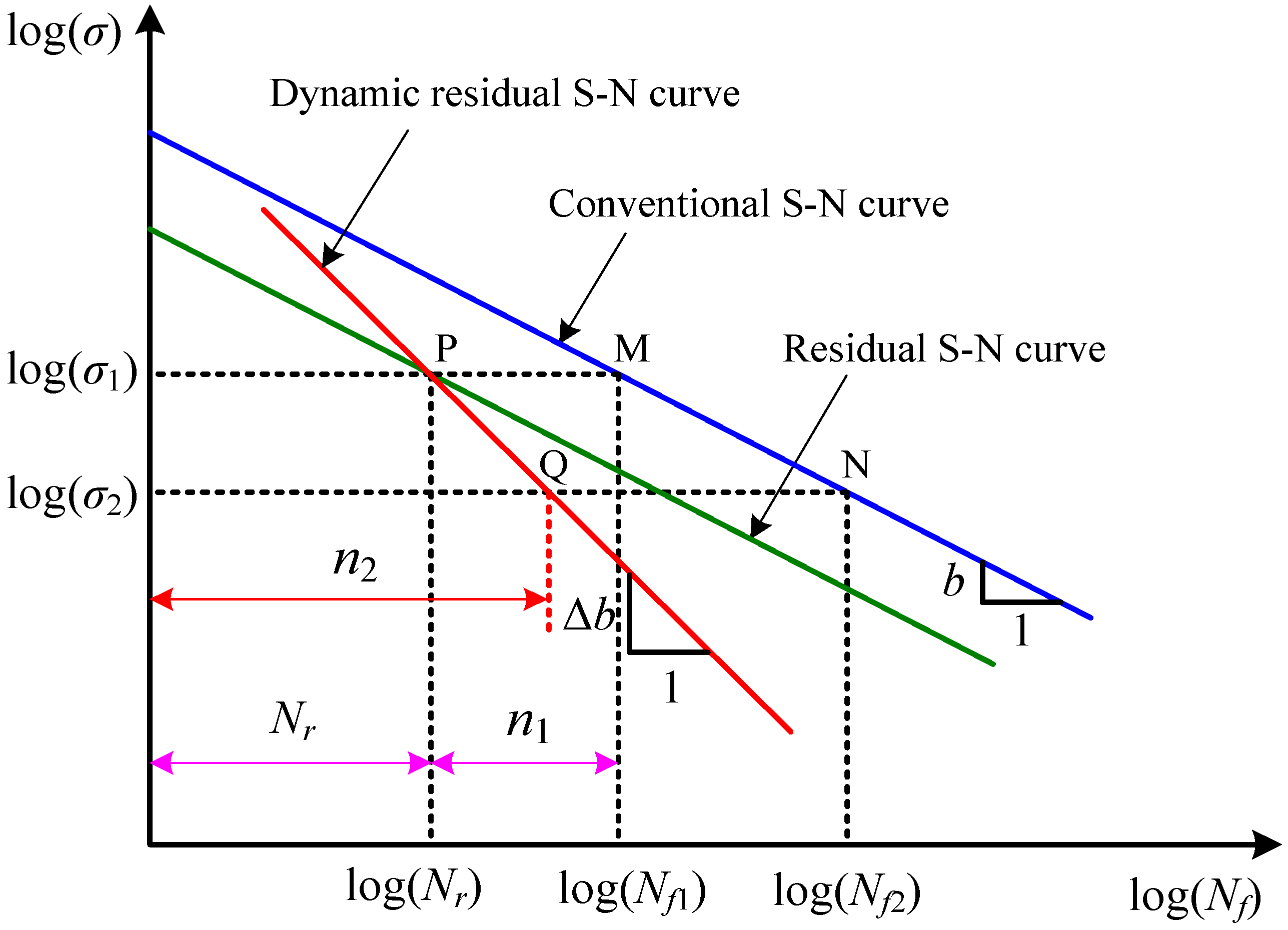
The usual way of analyzing and predicting fatigue life of metallic materials or components is to plot the stress amplitude against the number of loading cycles to failure, i.e., S-N diagram. It is widely accepted that the basic stress-life relation can be expressed by the Basquin’s power law [41], shown as:
where Nf is the number of loading cycles to failure at a given stress level σ; m and C are material constants; σ′f and h denote the fatigue strength coefficient and fatigue strength exponent, respectively. Equation (1) can be rewritten as a linear function in log-log coordinates, as shown in Figure 1, that is:
where a is the intercept and b is the slope (b = −1/m).
Given that a specimen suffers the initial damage induced by the loading stress amplitude σ1 for n1 cycles, the residual number of cycles to fracture (residual life Nr) at the same stress amplitude is (see Figure 1). For the undamaged specimen, the residual life corresponds to the fatigue failure cycles determined from the conventional S-N curve. Considering the damaged specimen as an undamaged one, a simple procedure for describing the stress-life relation of the damaged specimen is to use the residual S-N curve, which is assumed to have a similar mathematical description of the conventional one. Thus, a residual S-N curve with the same slope in Equation (2) can take the form:
where a′ is the intercept of residual S-N curve.
For variable amplitude loading tests, particular attention is often given to the commonly used and simplest case of the two-stage cyclic loading. Under laboratory loading condition, such loading pattern is defined as the procedure that the specimen is first pre-cycled at a certain stress amplitude σ1 for n1 cycles, then cycled at another stress amplitude σ2 for n2 cycles to failure. The relationship between Equations (2) and (3) means to a linear cumulative damage rule, that is:
According to this, Equation (3) is thus called the Miner’s residual S-N curve, because the slope in Equation (3) is the same as that in Equation (2). Since Equation (4) does not consider the effect of loading histories, the slope in Equation (3) may be a dominant factor of describing the loading effects on fatigue. In this work, the residual S-N curve slope is considered as a variable with respect to the previous fatigue loadings, instead of a basic material constant. Then, a dynamic residual S-N curve, as shown in Figure 1, can be expressed as:
where a′′ is the intercept and Δb is the dynamic slope.
The fatigue behaviors responsible for Equation (5) can be described as: for the material in virgin state without initial damage, Δb is identical to the original slope b; as the fatigue loading continues, the absolute value of Δb increases with the progressive fatigue damage; at fracture, it tends to be infinite. Consequently, the slope ratio b/Δb, which is defined as br for later convenience, will decrease with the loading cycles or the expended life fraction and should range from 1 to 0. In the dynamic residual S-N curve method, the change in slope is appropriate to present the fatigue failure process and the evolution law of damage accumulation. It is essential to quantify br when accumulating fatigue damage.
Recently, Böhm et al. [40,42] presented a material memory concept that was taken from the psychology domain for fatigue damage analysis. There are some similarities between the human memory and the material properties. In general, the human memory performance is described as an exponential function of time, for example the Ebbinghaus forgetting curve [43]. Through taking the fatigue loading cycles to replace the time function, their authors also suggested a material memory function as:
where M is the material memory performance; A is the memorization factor; B is the asymptote; d denotes the reverse of forgetting factor that is given by fatigue cycles and recommended as d = Nf for simplicity. The forgetting curve is shown in Figure 2.
From Equation (6), the performance measure of material memory degenerates progressively under the cyclic loading. At the initial state, i.e., n = 0, the memory performance is ; when the material is fatigued, it will decrease with the accumulated loading cycles, and ; at the critical state, i.e., n = Nf,. In order to present the degree of degradation, a decay coefficient of the material memory performance is introduced and simply described as follows:
It is noted that α is a function of the expended life fraction and varies from 1 to 0. For the initial condition, i.e., n/Nf = 0, α = 1, the material is undamaged without degeneration; after that, α decreases with the fatigue loading cycles; when n/Nf = 1, α = 0, the material will fully be degenerated. To a certain extent, this decay coefficient can correctly characterize the fatigue damage behaviors and the damaged degree of the material. As stated before, the slope ratio br in dynamic residual S-N curve is used to characterize the evolution law of damage accumulation. Thus, it is suitable to use the degeneration parameter of α to quantify br.
In the case of two-stage cyclic loading, the material is fatigued by the first stress amplitude σ1 for n1 cycles, and the slope in Equation (5) becomes Δb1. The change in slope from b to Δb1 represents the damage degree of the material, which can be characterized by the decay coefficient α. Besides, α satisfies the boundary conditions (it ranges from 1 to 0) with respect to b/Δb1. Therefore, the slope ratio for the first operation can be assumed as:
According to the conventional S-N curve in Figure 1, the points M (Nf1, σ1) and N (Nf2, σ2) should satisfy Equation (2), that is:
Subtracting Equation (10) from Equation (9) gives:
In the dynamic residual S-N curve, the residual life at the second stress amplitude σ2 is Nr2 = n2, and the points P (Nf1 − n1, σ1) and Q (n2, σ2) should satisfy Equation (5), that is:
Subtracting Equation (13) from Equation (12), we obtain:
Combing Equations (11) and (14) yields:
Substituting Equation (8) into Equation (15), the life fraction at the second loading level can be derived as:
For the high-low loading sequence (0 < Nf1/Nf2 < 1), the sum of the expended life fractions is:
For the low-high loading sequence (Nf1/Nf2 > 1), it is:
Considering that the final fracture occurs when the cumulative damage reaches a failure threshold of Df = 1, by rearranging Equation (16), one can obtain a failure criterion of cumulative damage as follows:
For a three-stage fatigue loading, using a similar analytical method and derivation procedure of the two-stage loading, the slope ratio and the life fraction at the third loading level can be expressed by Equations (20) and (21), respectively:
By rearranging Equation (21), it leads to the following failure criterion:
It should be pointed out that Equations (20) and (22) can be generalized to the multi-stage loading protocols. The representation of the slope ratio for the i-level fatigue loading is calculated by:
Accordingly, the cumulative damage criterion of fatigue failure can be derived as:
For each item in Equation (24), a general form of the damage variable Di is obtained as:
Therefore, a new cumulative fatigue damage rule yields:
Note that Equation (25) relates to the parameters of expended life fraction and fatigue failure lives, and they can be determined directly from the experimental data and conventional S-N curve. In Equation (24), fatigue damage is accumulated by taking a linear summation of the segmental damage caused by each loading stress level. For constant amplitude loading, Nf1 = Nf2 = … = Nfi and that Nfj/Nf(j+1) = 1, then Equation (26) degenerates to the Miner rule. Hence, Miner rule can be viewed as a particular case of the proposed model under constant amplitude loading. As a matter of fact, the proposed model improves the Miner rule by multiplying a load effect coefficient in connection with previous fatigue loadings to represent the loading sequence effect.
2.2. Typical Cumulative Damage Rules
In this study, three typical and commonly used cumulative damage rules, i.e., Palmgren-Miner rule, Corten-Dolan rule, and Kwofie-Rahbar rule, are chosen and briefly reviewed for analysis.
2.2.1. Palmgren-Miner Rule (Miner Rule for Short)
The initial treatment of cumulative fatigue damage is the LDR, i.e., Palmgren-Miner rule or Miner rule [17], with a basic assumption of constant work absorption in materials. In this rule, fatigue damage accumulates progressively in a linear manner, and the cumulative damage at failure is assumed as Df = 1. Mathematically, Miner rule can be expressed as:
The damage variable for each loading stress level is given by:
In Equation (28), the measure of fatigue damage is simply defined as a life fraction or cycle ratio. The load effect coefficient can be taken as unity without considering fatigue loading histories.
2.2.2. Corten-Dolan Rule (Corten’s Model for Short)
Corten-Dolan rule [25] is one of the earliest theories to predict load interaction effects by modifying the slope of conventional S-N curve. The rule hypothesizes that fatigue damage is a result of the nucleation of microscopic voids, which cause crack initiation and crack propagation. The damage is described as a function of the number of damaged nuclei, the rate of damage propagation, and the accumulated loading cycles. The theory predicts the failure criterion as follows:
where σi,max and Nfi,max denote the maximum loading stress level of applied loads and its fatigue life, respectively; d is a material parameter that is recommended as 4.8 for high strength steel and 5.8 for other materials.
Supposing that σi,max = σ1, Equation (29) can be rewritten as:
For each item in Equation (30), the damage variable is:
In this model, the life fraction is amplified by a load effect coefficient with respect to applied loads, fatigue lives, and the exponent d. If the d value is identical to the material constant m in Equation (1), Equation (30) reduces to Equation (27), i.e., Miner rule.
2.2.3. Kwofie-Rahbar Rule (Kwofie’s Model for Short)
Recently, Kwofie and Rahbar [31] proposed a fatigue driving stress concept to describe the damage accumulation process. The driving stress model is expressed by a function of expended life fraction, cyclic stress amplitude, and fatigue life. By using an equivalent driving stress approach similar to the equivalent damage rule [44], a cumulative damage model can be derived as follows:
For each stage of loading amplitudes, the damage variable is defined as:
In the model, a load effect coefficient associated with the fatigue lives of the current load and the initial load is introduced to present the loading sequence effects. In particular, for constant amplitude loading, Equation (32) is reduced as the Miner rule.
3. Experiments and Discussions
In this section, the results from a series of two-stage and multi-stage experimental investigations are used to validate the proposed model. For the purpose of model comparison, three commonly used damage models, i.e., Miner rule, Corten’s model, and Kwofie’s model, are also employed to compare with the proposed model on the predictive capability. According to the total amount of cumulative damage obtained by different models, the total fatigue life can be calculated by the following formula [45]:
where Npre denotes the predicted fatigue life. If the cumulative fatigue damage tends to unity (or the critical damage), then the predicted fatigue life should be close to the experimental result and the corresponding fatigue model becomes more effective.
3.1. Two-Stage Fatigue Loading
3.1.1. Results from Manson
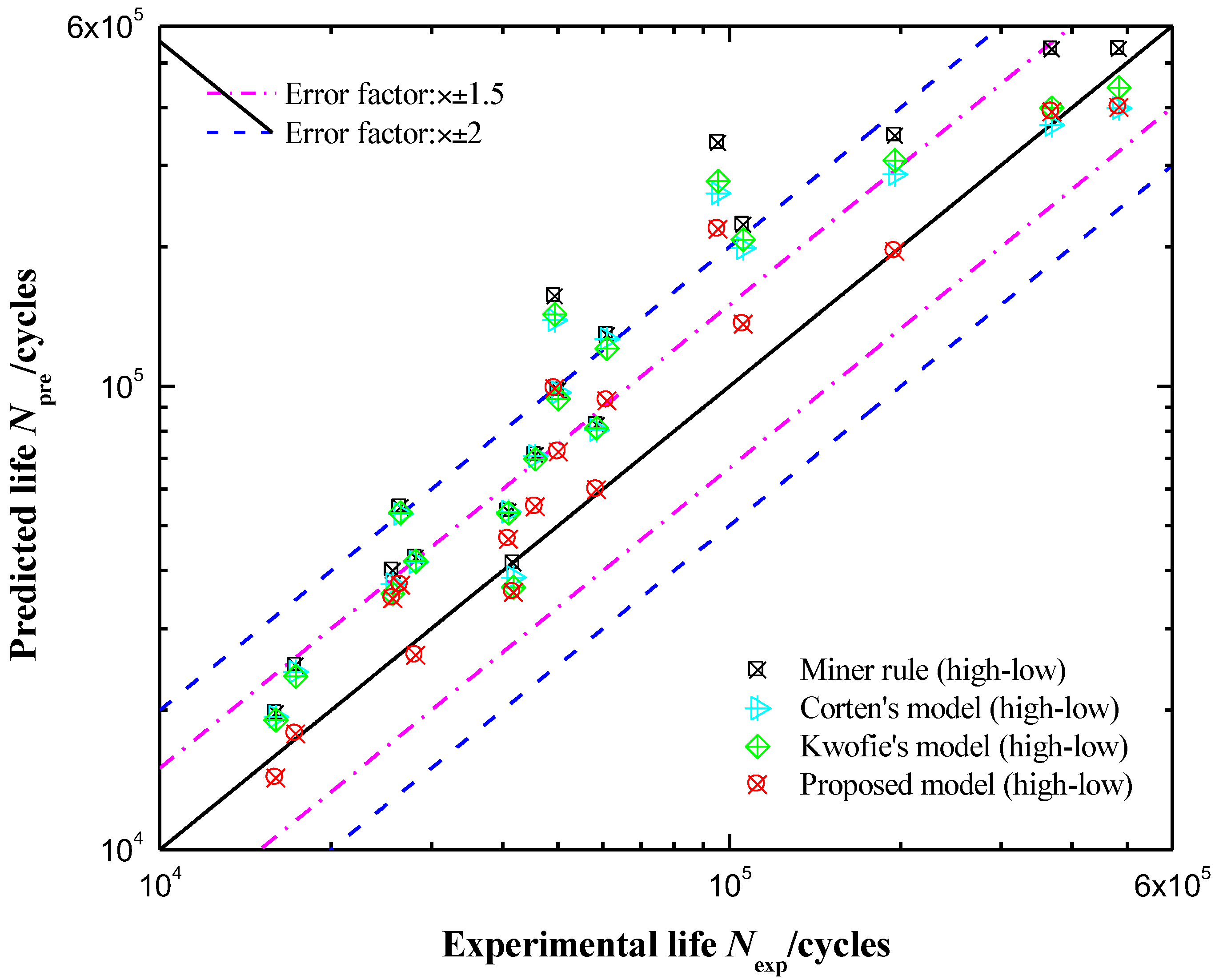
The test material used here is the maraging 300 CVM steel [46] with the following mechanical properties: yield strength σs = 2098 MPa, ultimate strength σb = 2590 MPa, and fatigue limit σf = 662 MPa. The tests were conducted on a rotating-beam fatigue machine under rotating bending loading. Four sets of high-low load spectrums were chosen, i.e., 1111–833 MPa, 1372–1111 MPa, 1303–751 MPa, and 1095–751 MPa. The fatigue lives of the loading stress amplitudes are determined from the S-N curve data as listed in Table 1. The comparisons between the experimental and predicted results are summarized in Table 2 (Nexp is the experimental fatigue life) and represented in Figure 3.
3.1.2. Results from Pavlou
The tested material is the Al-2024-T42 aluminum alloy [9], which has been widely used in aerospace design. The polished specimens were subjected to complete reverse bending loading for both high-low and low-high loading sequences with several configurations of specified fatigue cycles. The loading stress ratio is set to be R = −1. The applied stress amplitudes are 200 MPa and 150 MPa, and the corresponding fatigue lives are 150,000 cycles and 430,000 cycles, respectively. Two sets of two-stage load spectrums are 200–150 MPa for high-low loading and 150–200 MPa for low-high loading, respectively. The comparisons of the observed and theoretical results are shown in Table 3 and illustrated in Figure 4.
3.1.3. Results from Dattoma
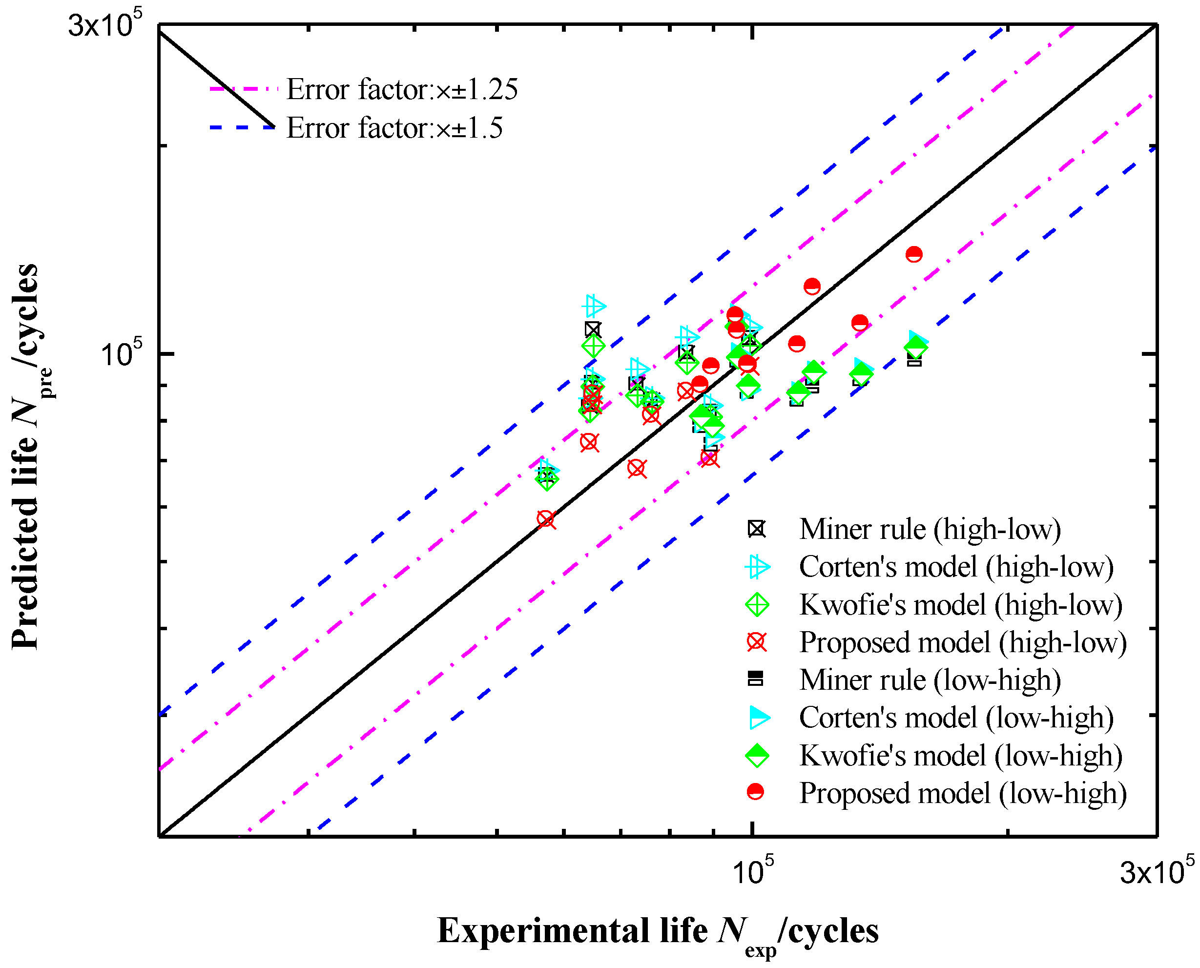
The material tested is a hardened and tempered 30NiCrMoV12 steel [47,48], which is mainly used for railway axle applications. The mechanical properties of the material are listed as: Young’s modulus E = 201.4 GPa, fatigue limit σf = 391 MPa, yield strength σs = 755 MPa, and ultimate strength σb = 1035 MPa. The tests were carried out on a servo-hydraulic MTS810 testing machine under oscillating tensile-compression loading in stress-controlled mode with R = −1. Five loading stress amplitudes are chosen, i.e., 485 MPa, 465 MPa, 450 MPa, 420 MPa, and 400 MPa, and their fatigue lives, determined from the S-N curve at 50% of probability of failure, are 54,998 cycles, 68,053 cycles, 80,330 cycles, 113,876 cycles, and 145,749 cycles, respectively. Three sets of two-stage high-low load spectrums are 485–400 MPa, 465–420 MPa, and 450–420 MPa, respectively. Three sets of two-stage low-high load spectrums are 400–485 MPa, 420–465 MPa, and 420–450 MPa, respectively. The comparisons between the observed results and models predictions are given in Table 4 and depicted in Figure 5.
To clearly show the predicted results, the scatter band is used to assess the predictive capability, as shown in Figure 2, Figure 3 and Figure 4. It is observed that the proposed model shows a good agreement between the experimental and theoretical results. From Table 2, Table 3 and Table 4, the cumulative damage calculated by the proposed model is found to be closer to unity than that of other models, and resulting in more accurate fatigue lives.
Among three typical damage models, the Miner rule has the simplest form that the segmental damage for each loading stress level is defined as a life fraction, but it fails to account for the effects of loading histories as a result of large prediction errors. The Corten’s model improves the Miner rule by modifying the S-N curve slope to consider load interaction effects, while the exploration of the predictions still shows a large deviation. This might be attributed to that the chosen value of the exponent d in Equation (31) is taken as an empirical constant, which is in reality independent of the loading histories. The Kwofie’s model is designed to consider the loading sequence effects, yet the predicted results by the model are slightly better than the counterparts from the Miner rule. It could be explained by the fact that the load effect coefficient in Equation (33) only relates to the initial and current fatigue lives, regardless of previous loading cycles on damage accumulation.
Through comparison with the above-mentioned models, the proposed model in the form of Equation (25) is closely linked to the expended life fractions and fatigue lives of previous loads. The model takes more fatigue loading history information into account and thus leads to relatively small prediction errors. It should be noted that the model follows a simple linear trend in accumulating fatigue damage and also accounts for load-level dependence and loading sequence effects. Consequently, the cumulative damage model presented here is expected to be reasonable and it should be easy to calculate damage and fatigue life using the conventional S-N curve data.
3.2. Multi-Stage Fatigue Loading
In order to further demonstrate the effectiveness of the proposed model, results from the multi-stage fatigue loading test data available in the literature are used. The tested material is 41Cr4 [45] with the following mechanical properties: ultimate strength σb = 850~900 MPa and fatigue limit σf = 173.5 MPa. Two sets of cumulative fatigue damage (CFD) tests, i.e., CFD1 test and CFD2 test, were performed under cyclic bending loading with R = −1. To check the capability of the predicted fatigue lives, the relative forecast error δ is employed and defined as follows:
3.2.1. Results from CFD1 Test
In the test, the cylindrical specimen was subjected to eight-stage high-low fatigue loading with six stress levels above the fatigue limit. The experimental fatigue life at fracture is Nexp = 2.00 × 10⁶ cycles. The loading test parameters and the predicted damage are listed in Table 5. A comparison of models prediction performances is shown in Table 6.
3.2.2. Results from CFD2 Test
The test was carried out under eight-stage high-low fatigue loading with five stress levels above the fatigue limit. The experimental fatigue life is Nexp = 2.20 × 10⁷ cycles. The models predictions and the corresponding prediction performances are shown in Table 7 and Table 8, respectively.
According to Table 6 and Table 8, it can be seen that the proposed model predicts the cumulative damage closer to unity and more accurate fatigue lives than three typical models. Table 5 and Table 7 list the segmental damage predicted by different models. It should be pointed out that the segmental damage caused by the stress levels below the fatigue limit is negligible.
From the above-mentioned two cases, the predictions using the Miner rule show a large deviation with the experimental data, due to the lack of loading history effects. The Corten’s model and the Kwofie’s model are also found to predict large deviations, because their load effect coefficients only relate to limited fatigue loadings. This may not be sufficient to characterize the complex behaviors of loading histories, especially for multi-stage variable loadings. It should be anticipated that the proposed damage model shows a high sensitivity to the details of previous fatigue loadings with more loading histories for consideration and thus predicts better results.
Furthermore, some common characteristics and fundamental properties of the chosen fatigue models can be extracted as follows:
- (1)
- In the models, the damage variable can be characterized by a general form available for different loading amplitudes. Fatigue damage is accumulated by adding up the segmental damage caused by each loading stress level. These models are essentially the LDRs, and this makes it convenient to calculate damage and fatigue life, compared with various non-linear theories.
- (2)
- Miner rule defines the damage variable as a life fraction regardless of loading histories accountability, while three typical damage models improve this basic rule by multiplying a load effect coefficient, which tends to consider previous fatigue loadings on damage accumulation.
- (3)
- For constant amplitude loading, the proposed model, Corten’s model, and Kwofie’s model will degenerate to the Miner rule. It can be concluded that the Miner rule forms a particular basis for these linear extensions and should be sufficient to assess fatigue damage under constant amplitude loading because loading history effects can be ignored under such loading condition.
The findings obtained in this study are based on the S-N curve approach and should be restricted to the applicable range of high-cycle fatigue regime. The proposed model is calibrated by the uniaxial fatigue experimental data, and may be extended to the field of multiaxial fatigue criterion. The model improves some of the shortcomings of the Miner rule, but the void response for low amplitude loads below the fatigue limit still remains [49]. The cumulative damage formula of Equation (26) can also be improved by adjusting the critical failure criterion (conventionally, Df = 1), depending on the material properties, external loads, and safety factor, for increased prediction accuracy and fatigue resistant design. The fatigue modeling presented here pertains to a deterministic methodology, whereas the fatigue process is stochastic in nature with various uncertainties [50,51,52], such as load variation, model parameters, and statistical errors. Therefore, further insights into these uncertainties on fatigue are still in demand.
4. Conclusions
In this paper, the S-N curve approach is used to deal with the development of variable amplitude fatigue damage. From the present comparisons between the published experimental data and theoretical results, some conclusions can be drawn as follows:
- (1)
- A phenomenological cumulative damage rule is proposed by incorporating a dynamic residual S-N curve and material memory concept to describe damage accumulation behavior. The model follows a linear trend in accumulating damage and also takes the load-level dependence and loading sequences into account. It predicts the damage and fatigue life with a small amount of data necessary from the conventional S-N curve.
- (2)
- The proposed model is calibrated and verified by a series of non-uniform fatigue loading protocols. Comparing with the commonly used damage rules, the model predicts the cumulative damage closer to unity and more accurate fatigue lives. The present damage formula shows a high sensitivity to the details of previous fatigue loadings with more loading histories for consideration.
- (3)
- Several common characteristics and fundamental properties of the chosen fatigue models are briefly discussed. Miner rule is improved by multiplying a load effect coefficient with respect to previous fatigue loadings for three typical damage models. In particular, the Miner rule is also found to form a general basis for these linear extensions under constant amplitude loadings.
Author Contributions
Formal analysis, J.Z.; Funding acquisition, Y.-F.L.; Methodology, Z.P.; Supervision, H.-Z.H.; Validation, Y.-F.L.; Writing—original draft, Z.P.; Writing—review & editing, H.-Z.H.
Acknowledgments
This study was sponsored by the National Natural Science Foundation of China under Grant No. 51775090.
Conflicts of Interest
The authors declare no conflict of interest.
References
- Chaboche, J.L. Continuous damage mechanics—A tool to describe phenomena before crack initiation. Nucl. Eng. Des. 1981, 64, 233–247. [Google Scholar] [CrossRef]
- Lubarda, V.A.; Krajcinovic, D. Damage tensors and the crack density distribution. Int. J. Solids Struct. 1993, 30, 2859–2877. [Google Scholar] [CrossRef]
- Voyiadjis, G.Z.; Kattan, P.I. A comparative study of damage variables in continuum damage mechanics. Int. J. Damage Mech. 2009, 18, 315–340. [Google Scholar] [CrossRef]
- Rejovitzky, E.; Altus, E. On single damage variable models for fatigue. Int. J. Damage Mech. 2013, 22, 268–284. [Google Scholar] [CrossRef]
- Peng, Z.; Huang, H.Z.; Wang, H.K.; Zhu, S.P.; Lv, Z. A new approach to the investigation of load interaction effects and its application in residual fatigue life prediction. Int. J. Damage Mech. 2016, 25, 672–690. [Google Scholar] [CrossRef]
- Hu, D.; Wang, R.; Fan, J.; Shen, X. Probabilistic damage tolerance analysis on turbine disk through experimental data. Eng. Fract. Mech. 2012, 87, 73–82. [Google Scholar] [CrossRef]
- Tanaka, K.; Mura, T. A dislocation model for fatigue crack initiation. J. Appl. Mech. 1981, 48, 97–103. [Google Scholar] [CrossRef]
- Fedelich, B. A stochastic theory for the problem of multiple surface crack coalescence. Int. J. Fract. 1998, 91, 23–45. [Google Scholar] [CrossRef]
- Pavlou, D.G. A phenomenological fatigue damage accumulation rule based on hardness increasing, for the 2024-T42 aluminum. Eng. Struct. 2002, 24, 1363–1368. [Google Scholar] [CrossRef]
- Naderi, M.; Khonsari, M.M. A thermodynamic approach to fatigue damage accumulation under variable loading. Mater. Sci. Eng. A-Struct. 2010, 527, 6133–6139. [Google Scholar] [CrossRef]
- Li, Y.F.; Lv, Z.; Cai, W.; Zhu, S.P.; Huang, H.Z. Fatigue life analysis of turbine disks based on load spectra of aero-engines. Int. J. Turbo Jet-Eng. 2016, 33, 27–33. [Google Scholar] [CrossRef]
- Yu, L.; Chen, H.; Zhou, J.; Yin, H.; Huang, H.Z. Fatigue life prediction of low pressure turbine shaft of turbojet engine. Int. J. Turbo Jet-Eng. 2017, 34, 149–154. [Google Scholar] [CrossRef]
- Hou, S.Q.; Cai, X.J.; Xu, J.Q. A life evaluation formula for high cycle fatigue under uniaxial and multiaxial loadings with mean stresses. Int. J. Mech. Sci. 2015, 93, 229–239. [Google Scholar] [CrossRef]
- Zhang, W.; Zhou, Z.; Zhang, B.; Zhao, S. A phenomenological fatigue life prediction model of glass fiber reinforced polymer composites. Mater. Des. 2015, 66, 77–81. [Google Scholar] [CrossRef]
- Fatemi, A.; Yang, L. Cumulative fatigue damage and life prediction theories: A survey of the state of the art for homogeneous materials. Int. J. Fatigue 1998, 20, 9–34. [Google Scholar] [CrossRef]
- Schijve, J. Fatigue of Structures and Materials; Springer Science & Business Media: Berlin, Germany, 2001. [Google Scholar]
- Miner, M.A. Cumulative damage in fatigue. J. Appl. Mech. 1945, 12, 159–164. [Google Scholar]
- Manson, S.S.; Halford, G.R. Practical implementation of the double linear damage rule and damage curve approach for treating cumulative fatigue damage. Int. J. Fract. 1981, 17, 169–192. [Google Scholar] [CrossRef] [Green Version]
- Liu, Y.; Mahadevan, S. Stochastic fatigue damage modeling under variable amplitude loading. Int. J. Fatigue 2007, 29, 1149–1161. [Google Scholar] [CrossRef]
- Mi, J.; Li, Y.F.; Peng, W.; Huang, H.Z. Reliability analysis of complex multi-state system with common cause failure based on evidential networks. Reliab. Eng. Syst. Saf. 2018, 174, 71–81. [Google Scholar] [CrossRef]
- Li, X.Y.; Huang, H.Z.; Li, Y.F.; Zio, E. Reliability assessment of multi-state phased mission system with non-repairable multi-state components. Appl. Math. Model. 2018, 61, 181–199. [Google Scholar] [CrossRef]
- Huang, H.Z.; Huang, C.G.; Peng, Z.; Li, Y.F.; Yin, H. Fatigue life prediction of fan blade using nominal stress method and cumulative fatigue damage theory. Int. J. Turbo Jet Eng. 2017. [Google Scholar] [CrossRef]
- Lv, Z.; Huang, H.Z.; Zhu, S.P.; Gao, H.; Zuo, F. A modified nonlinear fatigue damage accumulation model. Int. J. Damage Mech. 2015, 24, 168–181. [Google Scholar] [CrossRef]
- Zuo, F.J.; Huang, H.Z.; Zhu, S.P.; Lv, Z.; Gao, H. Fatigue life prediction under variable amplitude loading using a non-linear damage accumulation model. Int. J. Damage Mech. 2015, 24, 767–784. [Google Scholar] [CrossRef]
- Corten, H.T.; Dolan, T.J. Cumulative fatigue damage. In Proceedings of the International Conference on Fatigue of Metals, London, UK, 10–14 September 1956. [Google Scholar]
- Freudenthal, A.M.; Heller, R.A. On stress interaction in fatigue and a cumulative damage rule. J. Aerosp. Sci. 1959, 26, 431–442. [Google Scholar] [CrossRef]
- Subramanyan, S. A cumulative damage rule based on the knee point of the S-N curve. J. Eng. Mater. Technol. 1976, 98, 316–321. [Google Scholar] [CrossRef]
- Hashin, Z.; Rotem, A. A cumulative damage theory of fatigue failure. Mater. Sci. Eng. 1978, 34, 147–160. [Google Scholar] [CrossRef]
- Leipholz, H.H.E. On the modified S-N curve for metal fatigue prediction and its experimental verification. Eng. Fract. Mech. 1986, 23, 495–505. [Google Scholar] [CrossRef]
- EI Aghoury, I.; Galal, K. A fatigue stress-life damage accumulation model for variable amplitude fatigue loading based on virtual target life. Eng. Struct. 2013, 52, 621–628. [Google Scholar] [CrossRef]
- Kwofie, S.; Rahbar, N. A fatigue driving stress approach to damage and life prediction under variable amplitude loading. Int. J. Damage Mech. 2013, 22, 393–404. [Google Scholar] [CrossRef]
- Peng, Z.; Huang, H.Z.; Zhu, S.P.; Gao, H.; Lv, Z. A fatigue driving energy approach to high—cycle fatigue life estimation under variable amplitude loading. Fatigue Fract. Eng. Mater. 2016, 39, 180–193. [Google Scholar] [CrossRef]
- Mesmacque, G.; Garcia, S.; Amrouche, A.; Rubio-Gonzalez, C. Sequential law in multiaxial fatigue, a new damage indicator. Int. J. Fatigue 2005, 27, 461–467. [Google Scholar] [CrossRef]
- Aïd, A.; Amrouche, A.; Bouiadjra, B.B.; Benguediab, M.; Mesmacque, G. Fatigue life prediction under variable loading based on a new damage model. Mater. Des. 2011, 32, 183–191. [Google Scholar] [CrossRef]
- Aid, A.; Bendouba, M.; Aminallah, L.; Amrouche, A.; Benseddiq, N.; Benguediab, M. An equivalent stress process for fatigue life estimation under multiaxial loadings based on a new non linear damage model. Mater. Sci. Eng. A Struct. 2012, 538, 20–27. [Google Scholar] [CrossRef]
- Djebli, A.; Aid, A.; Bendouba, M.; Amrouche, A.; Benguediab, M.; Benseddiq, N. A non-linear energy model of fatigue damage accumulation and its verification for Al-2024 aluminum alloy. Int. J. Nonlinear Mech. 2013, 51, 145–151. [Google Scholar] [CrossRef]
- Benkabouche, S.; Guechichi, H.; Amrouche, A.; Benkhettab, M. A modified nonlinear fatigue damage accumulation model under multiaxial variable amplitude loading. Int. J. Mech. Sci. 2015, 100, 180–194. [Google Scholar] [CrossRef]
- Rege, K.; Pavlou, D.G. A one-parameter nonlinear fatigue damage accumulation model. Int. J. Fatigue 2017, 98, 234–246. [Google Scholar] [CrossRef]
- Pavlou, D.G. The theory of the s-n fatigue damage envelope: Generalization of linear, double-linear, and non-linear fatigue damage models. Int. J. Fatigue 2018, 110, 204–214. [Google Scholar] [CrossRef]
- Böhm, E.; Kurek, M.; Junak, G.; Cieśla, M.; Łagoda, T. Accumulation of fatigue damage using memory of the material. Procedia Mater. Sci. 2014, 3, 2–7. [Google Scholar] [CrossRef]
- Basquin, O.H. The Exponential Law of Endurance Tests; American Society for Testing and Materials: Phildelphia, PA, USA, 1910. [Google Scholar]
- Böhm, E.; Kurek, M.; Łagoda, T. Accumulation of fatigue damages for block-type loads with use of material memory function. In Solid State Phenomena; Trans Tech Publications: Zürich, Switzerland, 2015; Volume 224, pp. 39–44. [Google Scholar]
- Ebbinghaus, H. Memory; Columbia University, Teachers College: New York, NY, USA, 1913. [Google Scholar]
- Richart, F.E.; Newmark, N.M. A Hypothesis for the Determination of Cumulative Damage in Fatigue; American Society for Testing and Materials: Phildelphia, PA, USA, 1948. [Google Scholar]
- Li, M.; Otto, B. Anti-Fatigue Design for Structural Components; China Machine Press: Beijing, China, 1987. [Google Scholar]
- Manson, S.S.; Freche, J.C.; Ensign, C.R. Application of a double linear damage rule to cumulative fatigue. In Fatigue Crack Propagation; ASTM STP 415; American Society for Testing and Materials: Philadelphia, PA, USA, 1967. [Google Scholar]
- Dattoma, V.; Giancane, S.; Nobile, R.; Panella, F.W. Fatigue life prediction under variable loading based on a new non-linear continuum damage mechanics model. Int. J. Fatigue 2006, 28, 89–95. [Google Scholar] [CrossRef]
- Giancane, S.; Nobile, R.; Panella, F.W.; Dattoma, V. Fatigue life prediction of notched components based on a new nonlinear continuum damage mechanics model. Procedia Eng. 2010, 2, 1317–1325. [Google Scholar] [CrossRef]
- Zhou, J.; Huang, H.Z.; Peng, Z. Fatigue life prediction of turbine blades based on modified equivalent strain model. J. Mech. Sci. Technol. 2017, 31, 4203–4213. [Google Scholar] [CrossRef]
- Hu, D.; Ma, Q.; Shang, L.; Gao, Y.; Wang, R. Creep-fatigue behavior of turbine disc of superalloy GH720Li at 650 C and probabilistic creep-fatigue modeling. Mater. Sci. Eng. A-Struct. 2016, 670, 17–25. [Google Scholar] [CrossRef]
- Zheng, B.; Huang, H.Z.; Guo, W.; Li, Y.F.; Mi, J. Fault diagnosis method based on supervised particle swarm optimization classification algorithm. Intell. Data Anal. 2018, 22, 191–210. [Google Scholar] [CrossRef]
- Li, X.Y.; Huang, H.Z.; Li, Y.F. Reliability analysis of phased mission system with non-exponential and partially repairable components. Reliab. Eng. Syst. Saf. 2018, 175, 119–127. [Google Scholar] [CrossRef]
Figure 1.
Schematic representation of conventional S-N curve, residual S-N curve, and dynamic residual S-N curve.
Figure 1.
Schematic representation of conventional S-N curve, residual S-N curve, and dynamic residual S-N curve.

Figure 2.
The forgetting curve.
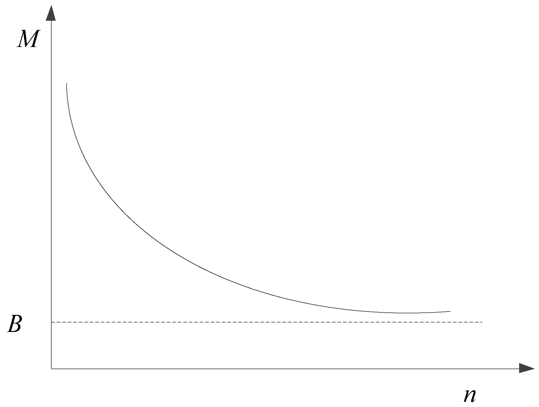
Figure 3.
Comparison between the experimental lives and the predicted lives by Miner rule, Corten’s model, Kwofie’s model, and the proposed model for maraging 300 CVM steel.
Figure 3.
Comparison between the experimental lives and the predicted lives by Miner rule, Corten’s model, Kwofie’s model, and the proposed model for maraging 300 CVM steel.

Figure 4.
Comparison between the experimental lives and the predicted lives by Miner rule, Corten’s model, Kwofie’s model, and the proposed model for Al-2024-T42 aluminum alloy.
Figure 4.
Comparison between the experimental lives and the predicted lives by Miner rule, Corten’s model, Kwofie’s model, and the proposed model for Al-2024-T42 aluminum alloy.

Figure 5.
Comparison between the experimental lives and the predicted lives by Miner rule, Corten’s model, Kwofie’s model, and the proposed model for 30NiCrMoV12 steel.
Figure 5.
Comparison between the experimental lives and the predicted lives by Miner rule, Corten’s model, Kwofie’s model, and the proposed model for 30NiCrMoV12 steel.


Table 1.
The loading stress amplitudes and their fatigue lives.
| Stress Amplitude (MPa) | 1372 | 1303 | 1111 | 1095 | 833 | 751 |
| Fatigue Life (Cycles) | 12,000 | 15,925 | 44,000 | 47,625 | 244,000 | 584,740 |
Table 2.
Experimental data and models predictions for maraging 300 CVM steel.
| Experimental Data | Predicted Results Using Different Models | |||||||||
|---|---|---|---|---|---|---|---|---|---|---|
| Miner Rule | Corten’s Model | Kwofie’s Model | Proposed Model | |||||||
| n1 | n2 | Nexp | Npre | ΣDi | Npre | ΣDi | Npre | ΣDi | Npre | ΣDi |
| High-low loading sequence: σ1 = 1111 MPa, σ2 = 833 MPa | ||||||||||
| 11,968 | 49,044 | 61,012 | 128,990 | 0.4730 | 126,630 | 0.4818 | 120,770 | 0.5052 | 93,120 | 0.6552 |
| 16,412 | 33,672 | 50,084 | 98,010 | 0.5110 | 96,870 | 0.5170 | 93,950 | 0.5331 | 72,190 | 0.6938 |
| 24,420 | 21,228 | 45,648 | 71,100 | 0.6420 | 70,680 | 0.6458 | 69,600 | 0.6559 | 54,940 | 0.8309 |
| 31,900 | 9028 | 40,928 | 53,710 | 0.7620 | 53,600 | 0.7636 | 53,300 | 0.7679 | 46,790 | 0.8747 |
| High-low loading sequence: σ1 = 1372 MPa, σ2 = 1111 MPa | ||||||||||
| 960 | 24,684 | 25,644 | 40,010 | 0.6410 | 37,440 | 0.6850 | 35,690 | 0.7186 | 34,800 | 0.7370 |
| 948 | 40,832 | 41,780 | 41,490 | 1.0070 | 38,700 | 1.0797 | 36,800 | 1.1354 | 35,900 | 1.1638 |
| 4944 | 12,364 | 17,308 | 24,980 | 0.6930 | 24,210 | 0.7150 | 23,650 | 0.7319 | 17,760 | 0.9745 |
| 7404 | 8580 | 15,984 | 19,680 | 0.8120 | 19,320 | 0.8273 | 19,050 | 0.8390 | 14,280 | 1.1194 |
| High-low loading sequence: σ1 = 1303 MPa, σ2 = 751 MPa | ||||||||||
| 971 | 367,810 | 368,781 | 534,470 | 0.6900 | 366,470 | 1.0063 | 399,030 | 0.9242 | 391,320 | 0.9424 |
| 1991 | 93,560 | 95,551 | 335,270 | 0.2850 | 261,430 | 0.3655 | 277,280 | 0.3446 | 218,350 | 0.4376 |
| 3790 | 45,610 | 49,400 | 156,330 | 0.3160 | 139,080 | 0.3552 | 143,190 | 0.3450 | 99,020 | 0.4989 |
| 7166 | 19,300 | 26,466 | 54,800 | 0.4830 | 52,970 | 0.4996 | 53,430 | 0.4953 | 37,260 | 0.7104 |
| 10,001 | 18,130 | 28,131 | 42,690 | 0.6590 | 41,700 | 0.6746 | 41,960 | 0.6705 | 26,280 | 1.0704 |
| High-low loading sequence: σ1 = 1095 MPa, σ2 = 751 MPa | ||||||||||
| 3953 | 479,500 | 483,453 | 535,390 | 0.9030 | 398,590 | 1.2129 | 441,950 | 1.0939 | 400,310 | 1.2077 |
| 11,811 | 183,610 | 195,421 | 347,720 | 0.5620 | 287,090 | 0.6807 | 307,700 | 0.6351 | 195,710 | 0.9985 |
| 15,192 | 90,640 | 105,832 | 223,270 | 0.4740 | 198,710 | 0.5326 | 207,470 | 0.5101 | 136,190 | 0.7771 |
| 31,575 | 26,900 | 58,475 | 82,480 | 0.7090 | 80,500 | 0.7264 | 81,250 | 0.7197 | 59,810 | 0.9777 |
Table 3.
Experimental data and models predictions for Al-2024-T42 aluminum alloy.
| Experimental Data | Predicted Results Using Different Models | |||||||||
|---|---|---|---|---|---|---|---|---|---|---|
| Miner Rule | Corten’s Model | Kwofie’s Model | Proposed Model | |||||||
| n1 | n2 | Nexp | Npre | ΣDi | Npre | ΣDi | Npre | ΣDi | Npre | ΣDi |
| High-low loading sequence: σ1 = 200 MPa, σ2 = 150 MPa | ||||||||||
| 30,000 | 259,100 | 289,100 | 360,020 | 0.8030 | 549,620 | 0.5260 | 337,730 | 0.8560 | 284,830 | 1.0150 |
| 233,400 | 263,400 | 354,510 | 0.7430 | 534,280 | 0.4930 | 333,000 | 0.7910 | 282,010 | 0.9340 | |
| 193,500 | 223,500 | 343,850 | 0.6500 | 504,510 | 0.4430 | 323,910 | 0.6900 | 276,270 | 0.8090 | |
| 60,000 | 90,300 | 150,300 | 246,390 | 0.6100 | 292,410 | 0.5140 | 238,950 | 0.6290 | 196,730 | 0.7640 |
| 98,250 | 158,250 | 251,590 | 0.6290 | 302,000 | 0.5240 | 243,840 | 0.6490 | 198,810 | 0.7960 | |
| 114,600 | 174,600 | 261,770 | 0.6670 | 320,960 | 0.5440 | 253,040 | 0.6900 | 202,550 | 0.8620 | |
| 90,000 | 86,000 | 176,000 | 220,000 | 0.8000 | 248,590 | 0.7080 | 215,160 | 0.8180 | 171,880 | 1.0240 |
| 42,300 | 132,300 | 189,540 | 0.6980 | 202,600 | 0.6530 | 187,130 | 0.7070 | 163,540 | 0.8090 | |
| 99,800 | 189,800 | 228,130 | 0.8320 | 261,790 | 0.7250 | 222,510 | 0.8530 | 173,810 | 1.0920 | |
| Low-high loading sequence: σ1 = 150 MPa, σ2 = 200 MPa | ||||||||||
| 86,000 | 138,000 | 224,000 | 200,000 | 1.1200 | 217,900 | 1.0280 | 214,350 | 1.0450 | 254,550 | 0.8800 |
| 147,000 | 233,000 | 197,460 | 1.1800 | 214,150 | 1.0880 | 211,820 | 1.1000 | 251,890 | 0.9250 | |
| 148,500 | 234,500 | 197,060 | 1.1900 | 213,570 | 1.0980 | 211,260 | 1.1100 | 251,610 | 0.9320 | |
| 172,000 | 138,000 | 310,000 | 234,850 | 1.3200 | 272,890 | 1.1360 | 249,000 | 1.2450 | 332,980 | 0.9310 |
| 139,500 | 311,500 | 234,210 | 1.3300 | 271,820 | 1.1460 | 248,210 | 1.2550 | 332,440 | 0.9370 | |
| 123,000 | 295,000 | 241,800 | 1.2200 | 284,750 | 1.0360 | 255,850 | 1.1530 | 337,920 | 0.8730 | |
| 258,000 | 89,000 | 347,000 | 290,860 | 1.1930 | 378,000 | 0.9180 | 303,060 | 1.1450 | 394,320 | 0.8800 |
| 81,000 | 339,000 | 297,370 | 1.1400 | 392,360 | 0.8640 | 309,310 | 1.0960 | 396,490 | 0.8550 | |
| 75,000 | 333,000 | 302,730 | 1.1000 | 404,130 | 0.8240 | 314,450 | 1.0590 | 398,330 | 0.8360 | |
Table 4.
Experimental data and models predictions for 30NiCrMoV12 steel.
| Experimental Data | Predicted Results Using Different Models | |||||||||
|---|---|---|---|---|---|---|---|---|---|---|
| Miner Rule | Corten’s Model | Kwofie’s Model | Proposed Model | |||||||
| n1 | n2 | Nexp | Npre | ΣDi | Npre | ΣDi | Npre | ΣDi | Npre | ΣDi |
| High-low loading sequence: σ1 = 485 MPa, σ2 = 400 MPa | ||||||||||
| 13,749 | 51,304 | 65,053 | 108,060 | 0.6020 | 117,190 | 0.5551 | 102,700 | 0.6334 | 87,310 | 0.7451 |
| 27,499 | 45,765 | 73,264 | 90,000 | 0.8140 | 94,880 | 0.7722 | 87,010 | 0.8420 | 68,090 | 1.0760 |
| 41,249 | 16,032 | 57,281 | 66,610 | 0.8600 | 67,760 | 0.8453 | 65,860 | 0.8698 | 57,390 | 0.9981 |
| High-low loading sequence: σ1 = 465 MPa, σ2 = 420 MPa | ||||||||||
| 17,013 | 66,845 | 83,858 | 100,190 | 0.8370 | 105,570 | 0.7943 | 97,040 | 0.8642 | 88,000 | 0.9529 |
| 34,027 | 30,405 | 64,432 | 84,010 | 0.7670 | 86,190 | 0.7476 | 82,670 | 0.7794 | 74,240 | 0.8679 |
| 51,040 | 38,262 | 89,302 | 82,230 | 1.0860 | 84,120 | 1.0616 | 81,070 | 1.1015 | 70,520 | 1.2664 |
| High-low loading sequence: σ1 = 450 MPa, σ2 = 420 MPa | ||||||||||
| 20,082 | 79,372 | 99,454 | 105,020 | 0.9470 | 109,030 | 0.9122 | 102,690 | 0.9685 | 95,860 | 1.0375 |
| 40,165 | 24,711 | 64,876 | 90,480 | 0.7170 | 91,870 | 0.7062 | 89,640 | 0.7237 | 84,300 | 0.7696 |
| 60,248 | 15,943 | 76,191 | 85,610 | 0.8900 | 86,290 | 0.8830 | 85,200 | 0.8943 | 81,290 | 0.9373 |
| Low-high loading sequence: σ1 = 400 MPa, σ2 = 485 MPa | ||||||||||
| 36,440 | 53,348 | 89,788 | 73,600 | 1.2200 | 75,660 | 1.1867 | 78,730 | 1.1405 | 95,550 | 0.9397 |
| 72,870 | 45,373 | 118,243 | 89,240 | 1.3250 | 93,960 | 1.2584 | 94,040 | 1.2574 | 124,490 | 0.9498 |
| 109,310 | 46,693 | 156,003 | 97,560 | 1.5990 | 104,060 | 1.4991 | 102,000 | 1.5294 | 138,500 | 1.1264 |
| Low-high loading sequence: σ1 = 420 MPa, σ2 = 465 MPa | ||||||||||
| 28,469 | 58,594 | 87,063 | 78,360 | 1.1110 | 79,670 | 1.0928 | 81,150 | 1.0729 | 89,840 | 0.9691 |
| 56,938 | 56,416 | 113,354 | 85,290 | 1.3290 | 87,690 | 1.2926 | 87,710 | 1.2923 | 102,890 | 1.1017 |
| 85,407 | 48,998 | 134,405 | 91,430 | 1.4700 | 94,960 | 1.4154 | 93,450 | 1.4382 | 110,300 | 1.2185 |
| Low-high loading sequence: σ1 = 420 MPa, σ2 = 450 MPa | ||||||||||
| 28,469 | 70,530 | 98,999 | 87,770 | 1.1280 | 88,750 | 1.1155 | 89,860 | 1.1017 | 96,390 | 1.0271 |
| 56,938 | 39,362 | 96,300 | 97,270 | 0.9900 | 99,790 | 0.9650 | 98,740 | 0.9753 | 107,680 | 0.8943 |
| 85,407 | 10,523 | 95,930 | 108,890 | 0.8810 | 113,720 | 0.8436 | 109,370 | 0.8771 | 113,140 | 0.8479 |
Table 5.
Experimental data and the predicted damage for CFD1 test.
| Stress Level | Stress Amplitude, σi (MPa) | ni (Cycles) | Nfi (Cycles) | Segmental Damage Caused by Each Stress Level | |||
|---|---|---|---|---|---|---|---|
| Miner Rule | Corten’s Model | Kwofie’s Model | Proposed Model | ||||
| 1 | 505 | 4 | 9.00 × 10³ | 0.0004 | 0.0004 | 0.0004 | 0.0004 |
| 2 | 475 | 32 | 1.16 × 10⁴ | 0.0028 | 0.0025 | 0.0029 | 0.0028 |
| 3 | 423 | 560 | 2.10 × 10⁴ | 0.0267 | 0.0223 | 0.0292 | 0.0268 |
| 4 | 362 | 5440 | 4.70 × 10⁴ | 0.1158 | 0.0877 | 0.1368 | 0.1206 |
| 5 | 287 | 40,000 | 1.55 × 10⁵ | 0.2580 | 0.1676 | 0.3387 | 0.3458 |
| 6 | 212 | 184,000 | 8.70 × 10⁵ | 0.2110 | 0.1328 | 0.3169 | 0.6645 |
| 7 | 137 | 560,000 | ∞ | 0 | 0 | 0 | 0 |
| 8 | 63 | 1,210,000 | ∞ | 0 | 0 | 0 | 0 |
Table 6.
Prediction performances of Miner rule, Corten’s model, Kwofie’s model, and the proposed model for CFD1 test.
Table 6.
Prediction performances of Miner rule, Corten’s model, Kwofie’s model, and the proposed model for CFD1 test.
| Prediction Performance | Experimetal Result | Miner Rule | Corten’s Model | Kwofie’s Model | Proposed Model |
|---|---|---|---|---|---|
| 1 | 0.6147 | 0.4133 | 0.8249 | 1.1609 | |
| Predicted fatigue life Npre (cycles) | 2.00 × 10⁶ | 3.25 × 10⁶ | 4.84 × 10⁶ | 2.42 × 10⁶ | 1.72 × 10⁶ |
| Relative forecast error δ (%) | — | 62.50 | 142.00 | 21.00 | 14.00 |
Table 7.
Experimental data and the predicted damage for CFD2 test.
| Stress Level | Stress Amplitude, σi (MPa) | ni (cycles) | Nfi (cycles) | Segmental Damage Caused by Each Stress Level | |||
|---|---|---|---|---|---|---|---|
| Miner Rule | Corten’s Model | Kwofie’s Model | Proposed Model | ||||
| 1 | 350 | 44 | 5.60 × 10⁴ | 0.0008 | 0.0008 | 0.0008 | 0.0008 |
| 2 | 332 | 352 | 7.40 × 10⁴ | 0.0047 | 0.0046 | 0.0048 | 0.0047 |
| 3 | 298 | 6160 | 1.30 × 10⁵ | 0.0475 | 0.0434 | 0.0512 | 0.0477 |
| 4 | 254 | 59,840 | 2.80 × 10⁵ | 0.2140 | 0.1667 | 0.2455 | 0.2290 |
| 5 | 201 | 440,000 | 1.25 × 10⁶ | 0.3520 | 0.3149 | 0.4520 | 0.6468 |
| 6 | 149 | 2,024,000 | ∞ | 0 | 0 | 0 | 0 |
| 7 | 96 | 6,160,000 | ∞ | 0 | 0 | 0 | 0 |
| 8 | 44 | 13,310,000 | ∞ | 0 | 0 | 0 | 0 |
Table 8.
Prediction performances of Miner rule, Corten’s model, Kwofie’s model, and the proposed model for CFD2 test.
Table 8.
Prediction performances of Miner rule, Corten’s model, Kwofie’s model, and the proposed model for CFD2 test.
| Prediction Performance | Experimetal Result | Miner Rule | Corten’s Model | Kwofie’s Model | Proposed Model |
|---|---|---|---|---|---|
| 1 | 0.6190 | 0.6631 | 0.7543 | 0.9290 | |
| Predicted fatigue life Npre (cycles) | 2.20 × 10⁷ | 3.55 × 10⁷ | 3.32 × 10⁷ | 2.92 × 10⁷ | 2.37 × 10⁷ |
| Relative forecast error δ (%) | — | 61.36 | 50.91 | 32.73 | 7.73 |
© 2018 by the authors. Licensee MDPI, Basel, Switzerland. This article is an open access article distributed under the terms and conditions of the Creative Commons Attribution (CC BY) license (http://creativecommons.org/licenses/by/4.0/).
Share and Cite
MDPI and ACS Style
Peng, Z.; Huang, H.-Z.; Zhou, J.; Li, Y.-F. A New Cumulative Fatigue Damage Rule Based on Dynamic Residual S-N Curve and Material Memory Concept. Metals 2018, 8, 456. https://doi.org/10.3390/met8060456
AMA Style
Peng Z, Huang H-Z, Zhou J, Li Y-F. A New Cumulative Fatigue Damage Rule Based on Dynamic Residual S-N Curve and Material Memory Concept. Metals. 2018; 8(6):456. https://doi.org/10.3390/met8060456
Chicago/Turabian StylePeng, Zhaochun, Hong-Zhong Huang, Jie Zhou, and Yan-Feng Li. 2018. "A New Cumulative Fatigue Damage Rule Based on Dynamic Residual S-N Curve and Material Memory Concept" Metals 8, no. 6: 456. https://doi.org/10.3390/met8060456
Note that from the first issue of 2016, this journal uses article numbers instead of page numbers. See further details here.