Flow-Accelerated Corrosion of Type 316L Stainless Steel Caused by Turbulent Lead–Bismuth Eutectic Flow


J-PARC Center, Japan Atomic Energy Agency, 2-4 Shirakata, Tokai-mura, Ibaraki 319-1195, Japan
*
Author to whom correspondence should be addressed.
Metals 2018, 8(8), 627; https://doi.org/10.3390/met8080627
Submission received: 4 July 2018
/
Revised: 2 August 2018
/
Accepted: 8 August 2018
/
Published: 9 August 2018
(This article belongs to the Special Issue Advances in Low-carbon and Stainless Steels)
Abstract
:Lead–bismuth eutectic (LBE), a heavy liquid metal, is an ideal candidate coolant material for Generation-IV fast reactors and accelerator-driven systems (ADSs), but LBE is also known to pose a considerable corrosive threat to its container. However, the susceptibility of the candidate container material, 316L stainless steel (SS), to flow-accelerated corrosion (FAC) under turbulent LBE flow, is not well understood. In this study, an LBE loop, referred to as JLBL-1, was used to experimentally study the behavior of 316L SS when subjected to FAC for 3000 h under non-isothermal conditions. An orificed tube specimen, consisting of a straight tube that abruptly narrows and widens at each end, was installed in the loop. The specimen temperature was 450 °C, and a temperature difference between the hottest and coldest legs of the loop was 100 °C. The oxygen concentration in the LBE was lower than 10−8 wt %. The Reynolds number in the test specimen was approximately 5 × 10⁴. The effects of various hydrodynamic parameters on FAC behavior were studied with the assistance of computational fluid dynamics (CFD) analyses, and then a mass transfer study was performed by integrating a corrosion model into the CFD analyses. The results show that the local turbulence level affects the mass concentration distribution in the near-wall region, and therefore, the mass transfer coefficient across the solid/liquid interface. The corrosion depth was predicted on the basis of the mass transfer coefficient obtained in the numerical simulation and was compared with that obtained in the loop. For the abrupt narrow part, the predicted corrosion depth was comparable with the measured corrosion depth, as was the abrupt wide part after involving the wall roughness effects in the prediction; for the straight tube part, the predicted corrosion depth is about 1.3–3.5 times the average experimental corrosion depth, and the possible reason for this discrepancy was provided.
1. Introduction
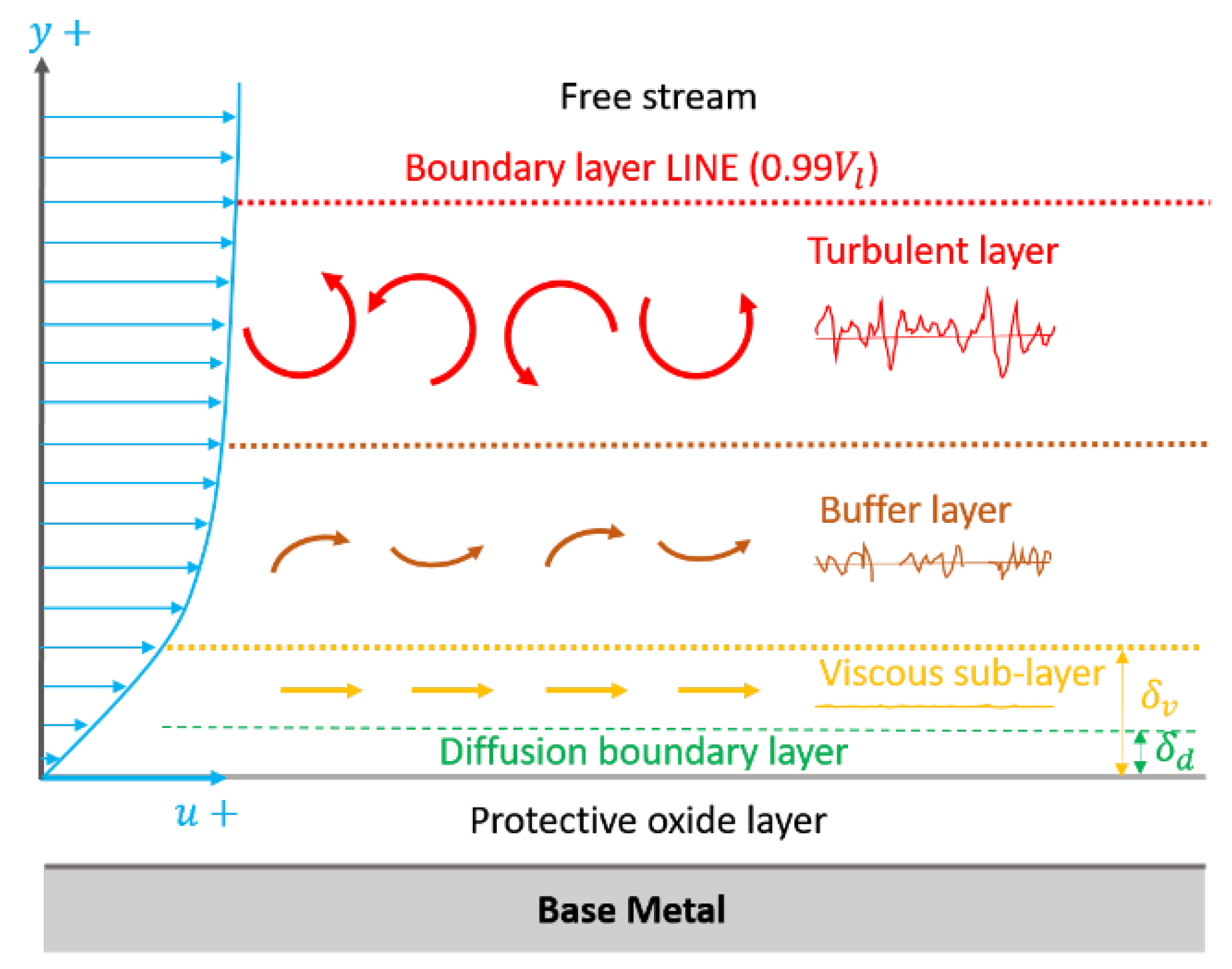
Flowing liquid has the potential to accelerate the rate at which metal corrodes, a phenomenon known as flow-accelerated corrosion (FAC). In fully developed turbulent flow in simple geometries (e.g., within a pipe) and a no-slip wall condition, the flow is halted at the solid wall, meaning that the flow will transition from turbulent in the bulk fluid to laminar very close to the wall. A so-called “hydro-dynamic boundary layer” will thus be formed, with its boundary line where the flow velocity equals 0.99 of the free stream flow velocity. The boundary layer can be divided into three typical layers depending on the correlation between the dimensionless velocity () and the dimensionless distance normal to the wall () with approach to the solid wall: (1) the turbulent flow layer, where and have a logarithmic correlation; (2) the buffer layer, where flow transition from turbulent to laminar occurs; and (3) the laminar flow layer, also known as the viscous sublayer, where is linearly proportional to , the turbulence level damps rapidly, and the viscous effects of fluid are dominant. If a dissolution constituent of a fluid has a high Schmidt number (), exceeding several hundreds, the mass diffusion boundary layer will be very thin, and will be embedded deep in the hydrodynamic viscous sublayer. The characteristics of the boundary layer are illustrated schematically in Figure 1 [1,2].
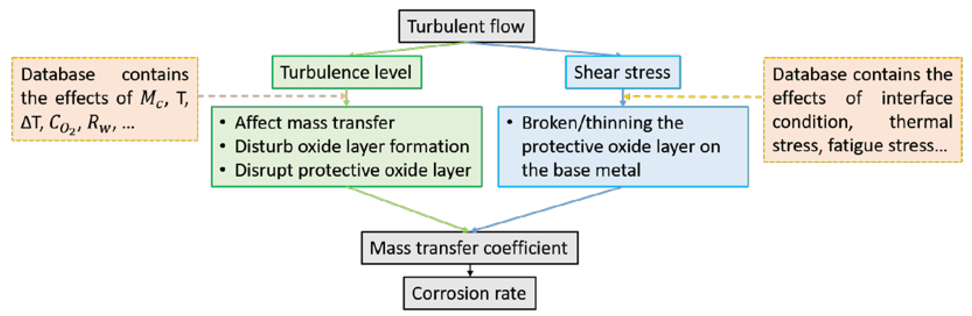
Pioneering studies have linked several hydrodynamic parameters, such as flow velocity [3], the Reynolds number [2], wall shear stress [4,5], and turbulence level [6] to the rate of FAC of metal. For turbulent flow in structures with simple geometries, the occurrence of FAC is mainly attributable to wall shear stress and the turbulence level in the near-wall region. The above two factors affect the protective oxide film on the base metal and the adjacent diffusion boundary layer [6], which are considered barriers to mass transfer, due to the particularly low mass transfer rate within them [7]. Fluctuations in turbulence can disturb the mass transfer rate from the bulk fluid to the metal surface and vice versa [5,8]; it can also disturb the formation of the protective oxide and disrupt the protective oxide layer [6]. Moreover, the shear stress generated at the wall may rupture or thin the protective oxide coating. In both cases, the mass transfer coefficient across the solid/liquid interface, and thus the corrosion rate of the metal, will be affected. In practice, the profile of wall shear stress and that of the near-wall turbulence level are coincident with each other for flow in structures with simple geometries because the shear stress on the wall is the main source of local turbulence [7]. This is shown schematically in Figure 2.
When flow encounters sudden contraction or expansion in pipes, orifices, valves, elbows, and weld heads, however, the hydrodynamic mechanisms of FAC become complex. In such situations, flow diversion and flow separations, flow reattachments, and flow recirculation occur. Extensive research has aimed at clarifying these mechanisms, but they are not yet thoroughly understood. Chang et al. [9] pointed out a positive correlation between wall shear stress and wall mass transfer. Utanohara et al. [10,11] concluded that the root mean square (RMS) of instantaneous shear stress is a suitable parameter for evaluating the FAC rate, despite their results showing a better correlation between the profiles of the FAC rate and the near-wall turbulence level. Their argument for discounting this result was that the relationship between the turbulence level and FAC had not been theoretically validated. Crawford et al. [12] indicated that the pressure drop attributed to secondary flow can significantly increase the average and oscillatory wall shear stress. By contrast, Nesic et al. [6,13] and Poulson [14] found that it is the high near-wall turbulence level, not the wall shear stress, which is responsible for localized enhancement in the wall corrosion rate. In addition, many other studies have linked the turbulence level to the rate of mass transfer and corrosion [15,16,17,18].
The majority of existing research has adopted water, sea water, or slurry as the flow medium, but a few studies have employed heavy liquid metals (HLMs), e.g., lead and lead-based alloys such as lead–bismuth eutectic (LBE). LBE is an ideal candidate coolant material for Generation-IV fast reactors and accelerator-driven systems (ADSs) because of the following physical characteristics: (1) a high boiling temperature, so that the heat generated in the reaction core can be utilized more efficiently; (2) its inertness on contact with water, air, and steam, enabling safe operation [19,20]. However, it is also well known that LBE poses a severe threat of corrosion on the material of its container [21], potentially ultimately leading to structural failure. The corrosion rate, , under LBE flows is a complex process involving many factors, and can be expressed as follows:
where is the chemical components of the test specimen, is the temperature of the test specimen, is the temperature difference between the hot and cold legs of a loop, is the oxygen concentration in the LBE, is the wall roughness, is the flow speed of the LBE, is the shear stress on the wall, and is the turbulence level in the near-wall region.
Earlier studies investigating the corrosion of structural steels by LBE looked at the loop as a whole, focusing on the corrosion pattern and the mass transfer behavior of the corrosion products [22]. The effects of and have attracted most attention [21,23]. There has also been a report of unexpected tube failure in the Corrosion In Dynamic lead Alloys (CORRIDA) loop at the Karlsruhe Institute of Technology [24]. A hole penetrated the tube, which had an initial wall thickness of 2.5 mm, downstream of a tube junction where the flowing LBE entered the vertical tube at an angle of 30 degrees. The study mentioning this attributed the failure to complex turbulent LBE flow. However, to the best of the authors’ knowledge, the local mechanism of FAC under turbulent LBE flow has not been studied in detail, either experimentally or numerically, from the perspectives of hydromechanics and wall mass transfer behavior.
If the potential of LBE as a coolant is to be exploited, it is highly desirable to investigate FAC of structural materials under turbulent LBE flow. To that end, the present study experimentally investigates FAC of type 316L stainless steel (SS), which is a candidate structural material for future ADSs, using the JLBL-1 loop installed at the Japan Atomic Energy Agency (JAEA). An orifice-type test tube with abrupt narrowing and widening at each end of a straight section was installed in the loop. Flow paths in the test tube show change in flow direction, fully developed flow, and recirculation. Investigations of the behavior of corrosion under such conditions are of interest and importance to scientific research and engineering applications. The study goes on to investigate the correlation between the hydrodynamic parameters and the corrosion profile using computational fluid dynamics (CFD) numerical simulations performed with STAR-CD. CFD analyses combined with a corrosion model are used to characterize the wall mass transfer behavior, and comparisons are drawn between the experimental and numerical results.
2. Physical Models
2.1. Turbulent Flow Model
The “standard” low Reynolds number (LRN) eddy-viscosity turbulence model in STAR-CD was adopted to model the flow and mass transfer [25]. The mass transfer is modelled by solving the mass transport equation together with the hydrodynamic equations, where the turbulent Schmidt number, , defines the ratio of turbulent momentum transport to turbulent diffusive transport. In the present study, was assigned a value of 0.9. The model is founded on the model proposed by Launder and Spalding [26], in which modelling of fully turbulent bulk flow is achieved through the transportation equations of turbulent kinetic energy (TKE), , and its dissipation rate, . Launder and Spalding model the near-wall region, where the viscous effect is dominant, by way of algebraic wall functions. However, this approach uses a velocity profile that is not applicable to recirculating flow, where there is flow separation and reversal, and does not take the detailed mass transfer characteristics in the diffusion boundary layer into account [27]. It is therefore necessary to use a turbulence model that directly solves the flow field and mass transfer deep inside the viscous sublayer to account for the changes due to the wall. The LRN model does so by solving the transport equations of and everywhere, including the near-wall regions.
To extend the high Reynolds number model to model low Reynolds number conditions, Lien et al. [28] have proposed damping functions that modify the transport equations of and in the near-wall region. One such is the semi-viscous near-wall effect , which modifies the eddy-viscosity term . An additional term for turbulence generation , which vanishes as approaches the order of 100, is added to ensure that the correct level of TKE dissipation is returned, and the destruction of TKE dissipation is modified with another damping factor . These are formulated as follows in STAR-CD:
where the turbulent Reynolds numbers are and .
2.2. Corrosion Model
In an isothermal closed liquid metal loop, corrosion may come to a halt because the corrosion products achieve saturation. However, in a non-isothermal loop where the saturation concentration of the corrosion products depends on temperature, continuous dissolution will occur in the relatively high-temperature part, whereas deposition of corrosion products will occur in the relatively low-temperature part. A kinetic equilibrium will be reached in which the amount of corrosion is balanced by the amount of deposition; thus, the precipitation sustains the corrosion [29]. This is particularly pertinent where metal corrosion occurs in an HLM environment, as this is a physical or physical-chemical process, which involves species dissolution, species transport, and chemical reaction between corrosion products and impurities, rather than an electrochemical process, as is usually the case in an aqueous environment [21,22].
In LBE environment, the corrosion process of a steel can be divided into two types according to the oxygen concentration in LBE [23,29]:
- (1)
- If the oxygen concentration in LBE is sufficiently low, as in the present experimental study, there will be no effective oxide protective layer formed on the steel surface. In this situation, the steel contacts with the LBE directly, and the main constituents of the steel are thus dissolved into the LBE directly.
- (2)
- If the oxygen concentration is within an appropriate range, oxidation of steel will occur, and an active oxide film (-based) will eventually be formed on the steel surface. Direct dissolution of steel into LBE will be prevented due to separation of the oxide film. In this case, the iron diffuses from the base metal, and the oxygen transfers from the bulk flow to the oxide/LBE interface to engage in the oxidation–reduction chemical reaction ().
For long-term steady-state LBE loop operation without an oxide protective layer, the steel corrosion process in the control depends on the LBE flow speed. If the LBE flow speed is rapid enough, resulting in the mass transfer rates of constituents in liquid greater than their dissolution reaction rates at the solid/LBE interface, then the corrosion will be controlled by the dissolution rate; otherwise, it will be controlled by the mass transfer rate in fluid [21,23]. For the mass transfer-controlled corrosion, if the diffusion flux of the corrosion product in the solid is less than the mass transfer rate in the liquid, surface recession will consequently occur [22].
The selective corrosion of Cr and Ni in the steel superficial layer is common for a 316L SS contacting with LBE that contains a low oxygen concentration. Subsequently, a phase change from austenite to ferrite might occur in the selective corrosion layer, due to the depletions of Cr and Ni in this layer, and as a result, a ferritic layer might be formed on the steel surface, where the concentrations of Cr and Ni are considerably low [30,31]. Both austenite and ferrite crystal mainly consist of iron, so that the dissolution of iron atoms will liberate other element atoms of the crystal into LBE, and therefore, it is reasonable to assume that the corrosion rate of iron determines the surface recession rate [22,32]. Hereafter, the surface recession rate is referred to as corrosion rate (CR) and the surface recession depth is called corrosion depth. The concentration of Cr and Ni in the solid at the solid/LBE interface can be assumed to be zero [22]. By contrast, the concentration of Fe in the solid at the solid/LBE interface is assumed to be equal to its saturation solubility in LBE, which will be described and discussed in detail in Section 4.2.
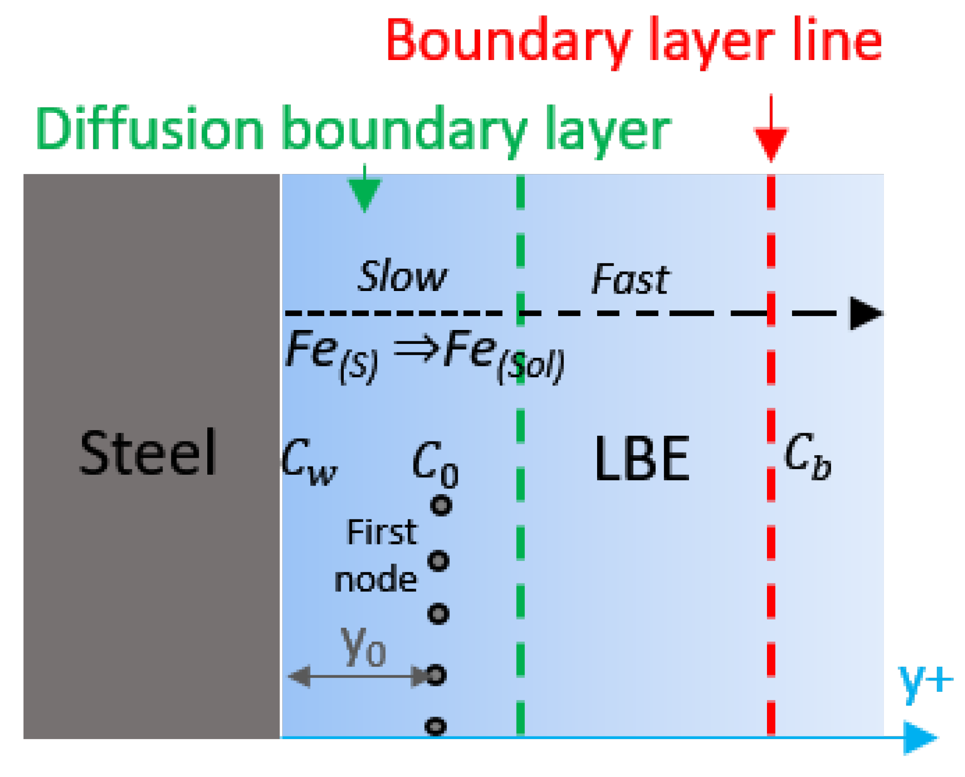
The corrosion process is illustrated schematically in Figure 3, and described by the following expression [33]:
The dissolved iron is transferred into the diffusion boundary layer, where the transfer of iron is governed by the molecular diffusion process, and thus, the transfer rate is low. Above the diffusion boundary layer in the viscous sublayer, where the transfer rate of iron grows dramatically. The thickness of the viscous sublayer is determined by the turbulence level of LBE flow, while the thickness of the diffusion boundary layer for each constituent is determined by not only the turbulence level of LBE flow, but also the Schmidt number () of each constituent. Therefore, the thickness of diffusion boundary layers of each constituent are independently different from each other. Therefore, lack of Ni and Cr involvement in the present corrosion model has insignificant effects on the thickness of the viscous sublayer and the diffusion boundary layer of Fe.
For a fully developed flow in a simple geometry, the mass transfer coefficient of a constituent across the wall can be indicated by the Sherwood number, . However, for complex geometries, there are no such empirical relationships, and CFD analysis must be used to aid its calculation.
The mass flux of iron, , from the reaction location to the bulk flow can be given by
where is the mass transfer coefficient, is the concentration of iron at the wall, and is the concentration of iron in the bulk fluid. In the simulation, if the first node (the layer of node closest to the wall in the mesh structure) is located in the diffusion boundary layer, then mass transfer between the wall and the first node is controlled solely by molecular diffusion. The effects of locations of the first node are insignificant, and can be positioned extremely close to the wall or at the end of the diffusion boundary layer. According to Fick’s law, the mass flux between the wall and the first node can be expressed as
where is the distance from the wall to the first node, is the molecular diffusion coefficient of iron, and is the iron concentration at the first node.
As mentioned previously, the rate of mass transfer in the diffusion boundary layer is very low, so it controls the total rate of mass transfer from the wall to the bulk flow. Therefore, the mass flux of iron is the same in Equations (7) and (6). By substituting Equation (7) into Equation (6), the mass transfer coefficient can be expressed as
In diffusion-controlled mass transfer, the diffusion coefficient of iron to or from the reaction site controls the rate of corrosion. The corrosion rate (in mm/h) can thus be defined as follows [34,35]:
where is the molar mass of iron, and is the density of iron. In the above equation, can be obtained in the numerical simulation by solving the mass transport equations described in the last subsection.
3. Experiments
3.1. JLBL-1
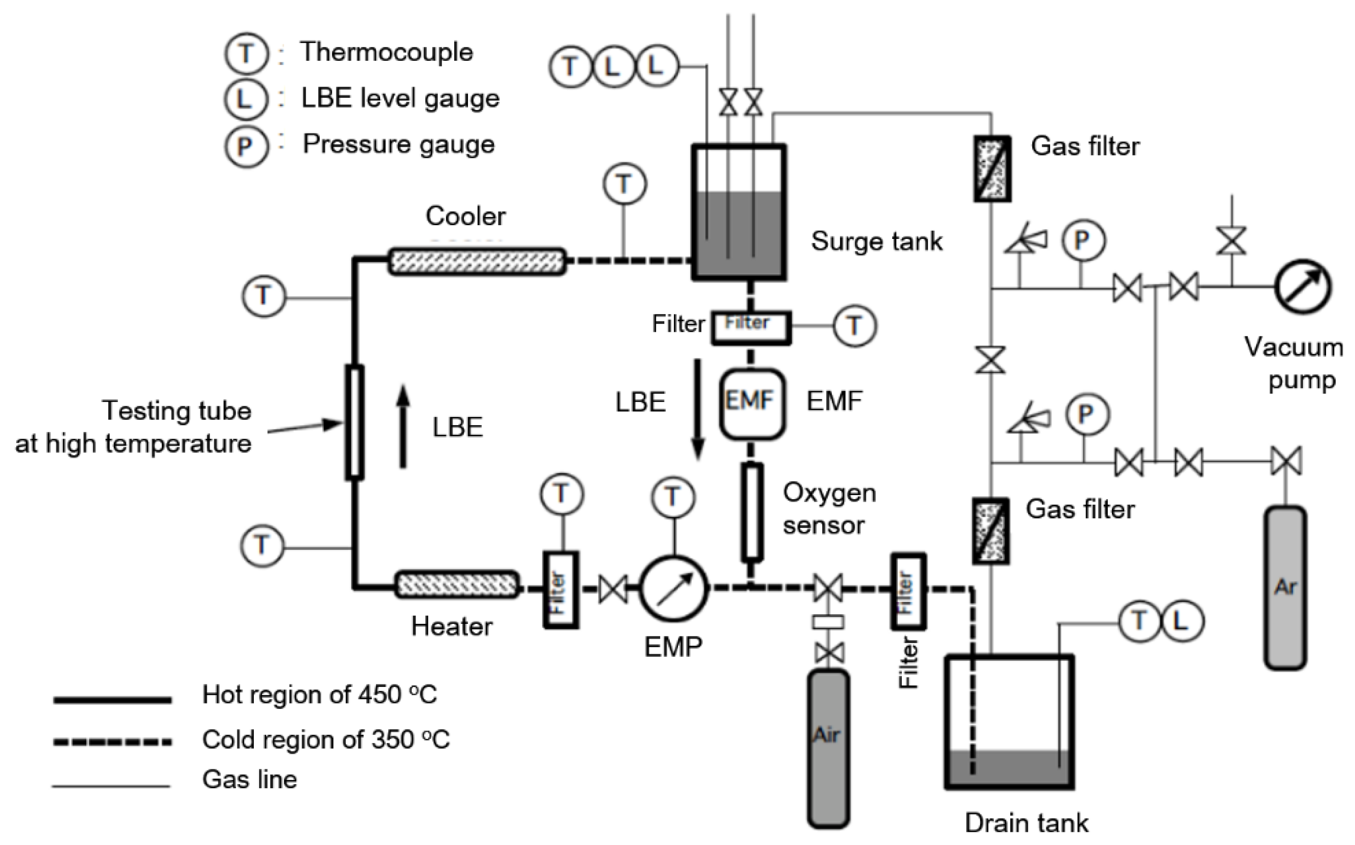
A corrosion test was performed with the JLBL-1 loop as specified in detail by Kikuchi et al. [36,37]. Flow in the loop is illustrated diagrammatically in Figure 4. The main circulating loop consists of an electromagnetic pump (EMP), a heater, a testing tube at high temperature (shown in Figure 5), LBE filters, a surge tank, a cooler, an electromagnetic flow meter (EMF), a surface-level meter, thermocouples, an observation window, and a drain tank. The JLBL-1 loop, including its main components, was manufactured by Sukegawa electric Co., Ltd., Takahagi, Japan. The LBE filters consist of thin, curling 430 SS foils. The EMP is linear inductive and has an annular channel. The EMF has two electrodes in contact with the LBE that detect electromotive force in the magnetic fields.
The tube and tanks that come into contact with lead–bismuth in the loop are made of 316L SS, and the tubes in the circulating loop, except for the testing tube, are 2.5 mm-thick cold-drawn products with an outer diameter of 27.2 mm. This means that the maximum velocity of the LBE will occur in the high-temperature specimen. The chemical composition of LBE is Pb-45/Bi-55 (wt %).
3.2. Specimen Testing Tube
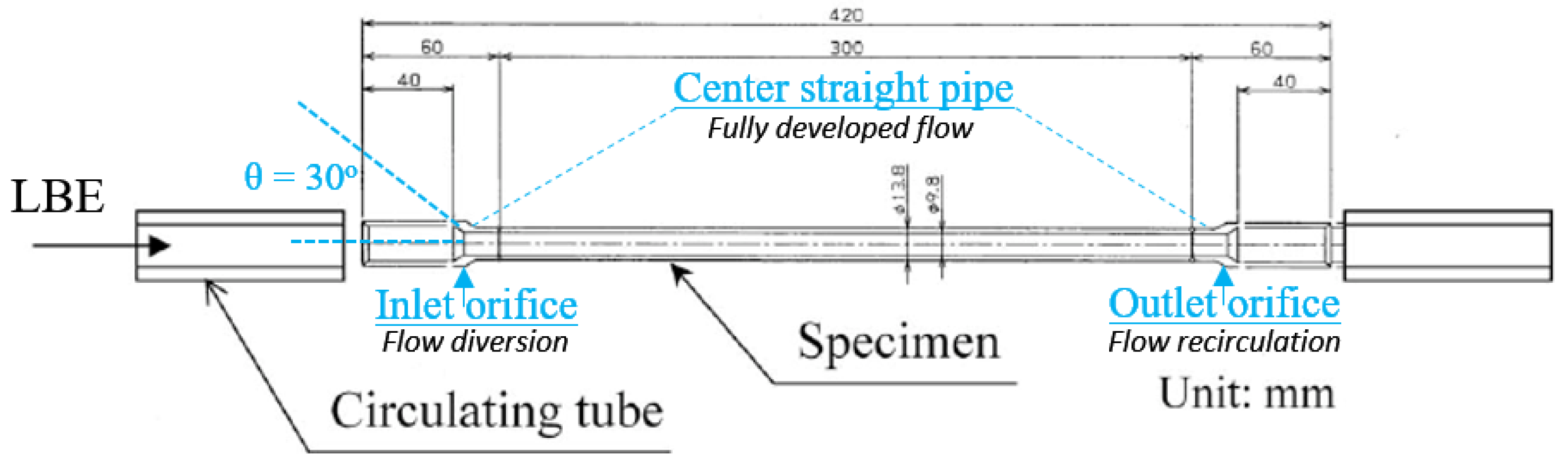
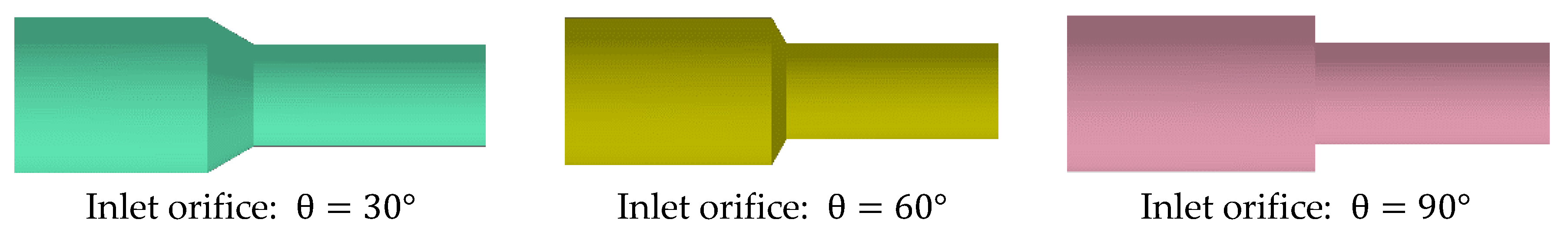
Figure 5 shows the testing tube. The testing tube is positioned downstream of the loop heater, as shown in Figure 4. The testing tube consists of an inlet orifice, a straight section, and an outlet orifice. The orifices are at 30° to the horizontal axis of the testing tube. The testing tube was machined from solution-annealed 316L SS plate as a tubing form of 2 mm thick, 40 cm long, and 13.8 mm outer diameter. The fabrication tolerance of the outer diameter and wall thickness is ±0.2 mm.
The chemical composition (wt %) of the type 316L austenitic SS used in this study is 16.84 Cr, 10.29 Ni, 0.73 Si, 1.02 Mn, 0.036 C, 0.030 P, and 0.005 S, balanced with Fe. The tube was solution heat-treated at 1080 °C for 1.5 h, and then cooled in water rapidly. The inner surface of the tube was polished to remove the rough layer after acid washing.
3.3. Operation Conditions
The temperature of the high- and low-temperature parts of the loop were 450 °C and 350 °C, respectively. The test duration was approximately 3000 h. The LBE flow rate was 5 L/min, corresponding to an average velocity of 0.7 m/s in the 9.8 mm diameter high-temperature testing tube. The flow rate was measured using an electromagnetic flowmeter (EMF). An oxygen sensor was placed in the loop, but did not work well, so the oxygen concentration in the LBE was neither measured nor controlled in this study. The literature [38] indicates that when the oxygen concentration is properly controlled to between 10−4 wt % and 10−7 wt %, an oxide film, with a thickness of several micrometers to tens of micrometers, will form on the surface of the stainless steel. Below that concentration range, no oxide film is formed. We can thus deduce that the oxygen concentration in the present experiment is below 10−8 wt %.
3.4. Post-Testing Material Characterization
After 3000 h, the specimens were cut out of the testing tube. The specimens were washed with silicon oil then cleaned with ethanol in an ultrasonic bath. They were then mounted in resin. After polishing, optical macroscopic (OM) and scanning electron microscopy (SEM) observations were carried out on the cross-sections of the specimens.
4. Numerical Simulation Conditions
4.1. Hydrodynamic Study
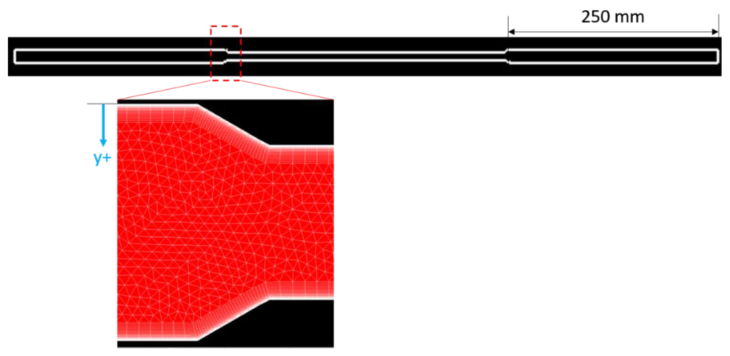
Steady-state CFD analysis was performed with the commercially available STAR-CD code. A half 3-dimensional (3D) model was meshed as shown schematically in Figure 6. To obtain a fully developed flow profile for the test tube, the length of each side of the specimen was extended to 250 mm in the simulations. All other dimensions are as in the specimen. The meshes were composed of tetrahedral cells, which were 0.75 mm in the straight part and 0.1875 mm in the two orifice sections. To study the hydrodynamic effects, it is necessary to understand the flow behavior deep in the viscous sublayer. This can generally be achieved by placing the first node at around y+ = 1. In this study, 45 layers of prism cells were meshed in the near-wall region. The distance of the first node of the prism layer from the wall is about 1.6 μm, corresponding to, approximately, y+ = 0.5. The expansion ratio of the prism layer is 1.1. There are approximately 7.6 million cells in the fluid field in total. The uniform flow speed at the inlet is 0.25 m/s, making the flow speed in the straight part approximately 0.7 m/s, which corresponds to that in the experiment. Good wettability is assumed for contact between LBE and the wall during the 3000 h operation, so the wall boundary is considered to be no-slip for the simulation. The LRN turbulence model was adopted to obtain detailed flow characteristics in the near-wall region using the equations detailed in Section 2.1. In addition, hydrodynamic simulation was performed to study the effects of the corroded morphology and angle of the orifices.
4.2. Mass Transfer Study
The mass transfer behavior of iron was investigated by integrating with the turbulent flow of LBE. A much finer mesh in the near-wall region is required to study the mass diffusion behavior from the wall to the bulk flow than for the hydrodynamic study, because it is necessary to place the first node in the diffusion boundary layer. In the mass transfer study, the first node of the prism layer is placed about 0.34 μm from the wall, corresponding to approximately y+ = 0.1, the recommended value for mass transfer studies [27]. Fifty layers of prism cells are placed beside the wall. The cell size is 0.75 mm.
As described in Section 2.2, for a long term non-isothermal closed loop, the concentration of iron in the bulk fluid cannot exceed its saturation concentration at the lowest temperature, or it will deposit on the coldest part of the wall. On the other hand, the concentration of iron increases as operation continues. Therefore, it is reasonable to assume that the iron concentration in the bulk fluid equals its saturation point at the lowest temperature [22,23]. The iron concentration at the wall in the hottest part depends on the situation. If the oxygen concentration is high enough that an -based protective film forms on the metal surface, the film can be reduced by the lead in the fluid. As a result, the equilibrium concentration of iron on the wall surface is controlled by this chemical reaction. However, if the oxygen concentration is sufficiently low that no oxide film forms, the equilibrium concentration of iron on the wall equals its saturation concentration [29]. Therefore, the concentrations of iron at the solid/liquid interface and in the bulk fluid are about 8.978 × 10⁻⁵ wt % and 9.576 × 10⁻⁶ wt %, respectively [39]. The molecular diffusion coefficient of iron in LBE is only known at certain temperatures, and has a large degree of scatter, and there is no diffusion coefficient of iron in LBE at 450 °C [38]. In this study, the iron diffusion coefficient in LBE is approximated to that of pure lead, as the diffusion coefficients of the two are considered to be similar [40,41]. Therefore, it is extrapolated from Robertson’s law that the molecular diffusion coefficient of iron in LBE at 450 °C is approximately 3.16 × 10⁻¹⁰ m2/s [38,41].
5. Results and Discussion
5.1. Corrosion Depth Profile of the Test Tube
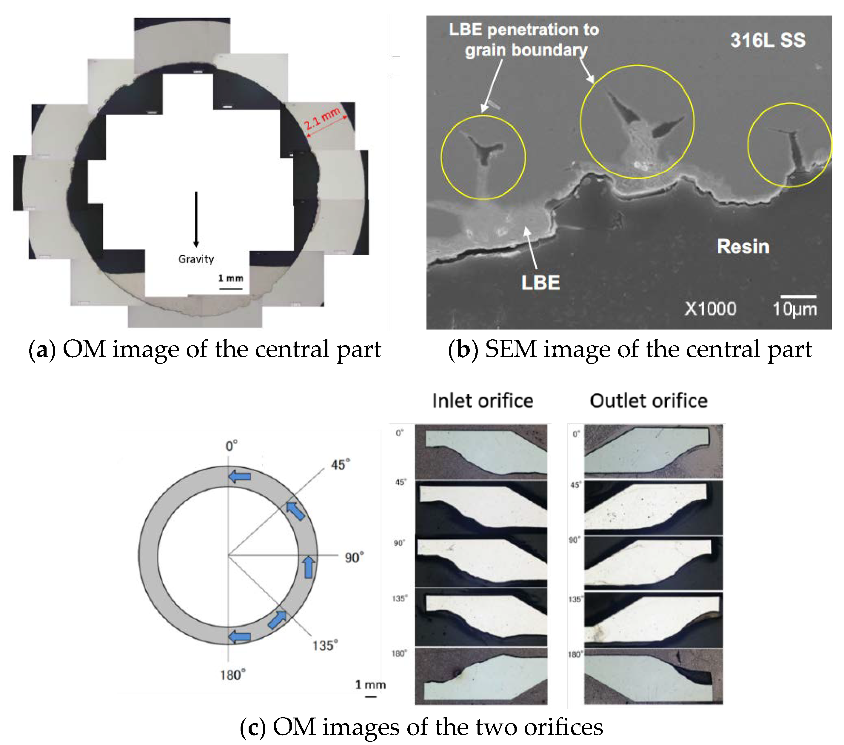
Figure 7a shows an OM image of cross-section of the specimen of the central straight pipe. The corrosion depth around the pipe circumference is relatively uniform. The maximum wall thickness of the corroded specimen is about 2.1 mm, as marked, which represents that the wall thickness of the as-received tube is no less than 2.1 mm. The fabrication tolerance is ±0.2 mm, so that the wall thickness of the as-received tube ranges from 2.1 to 2.2 mm, and it deviates 0.1–0.2 mm from its design size shown in Figure 5. This also implies that the thickness of the two 30-degree orifices deviates 0.087–0.173 mm from the design size. The corrosion depth of the specimen of the central straight pipe reaches a maximum of approximately 0.2–0.3 mm, and is 0.06–0.16 mm on average. The average corrosion rate ranges from 0.02 to 0.053 μm/h. Figure 7b shows the SEM image of cross-section of the specimen of the central straight pipe. No oxide film was observed on the specimen surface. Furthermore, there is LBE penetration into the grain boundary, which illustrates a typical corrosion scenario of 316L SS in LBE as stated previously in the corrosion model (Section 2.2). That is, Ni and Cr dissolve into LBE in the superficial area of the steel, and vacancies in the steel matrix are created as a result of depletion of Ni and Cr and of lower Fe content as well, and subsequently, Pb and Bi penetrate into the steel to fill the vacancies. During the ongoing penetration, selective leaching of Ni and Cr continues [38].
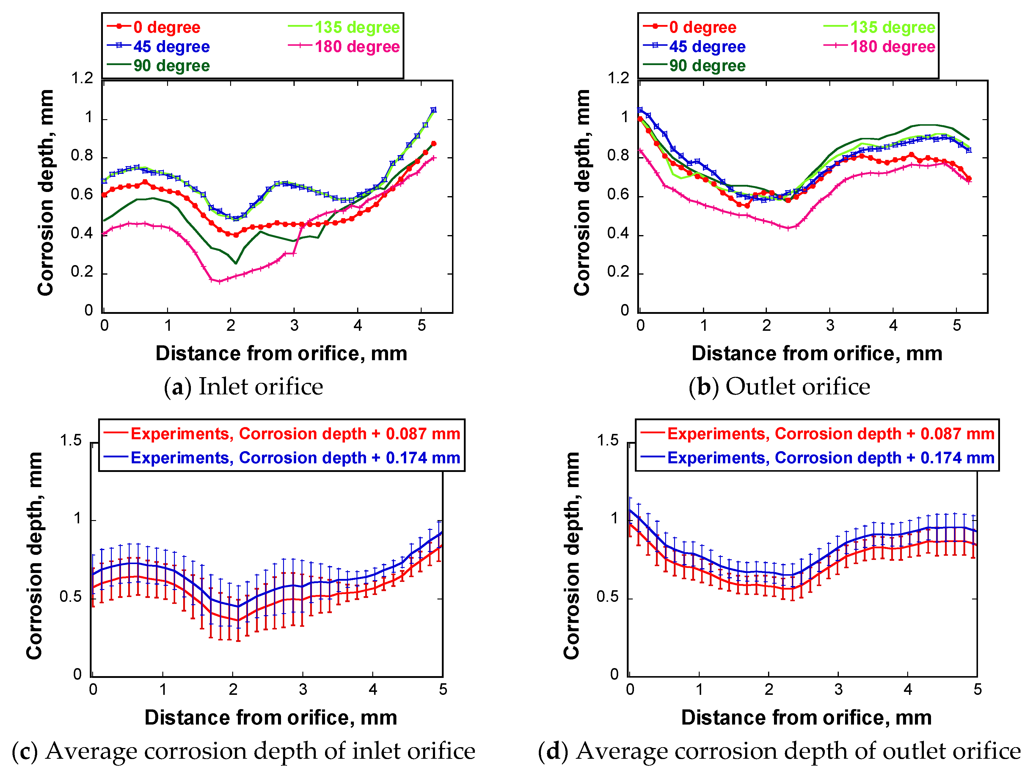
Figure 7c shows the OM images of cross-sections of the two orifices at various circumferential angles. The two orifices are the sloping parts seen in Figure 5. Clearly, the two orifice parts have been severely corroded, and the corrosion profiles are not uniform along the orifice surface. The quantitative corrosion depths of the two orifices along the orifice surface at various circumferential angles are plotted in Figure 8a,b. The corrosion depth was measured from the OM images by comparing the morphologies of the corroded orifice surfaces to those of the original surfaces. Each corrosion depth profile consists of forty datapoints measured equidistantly along the original orifice surface. The deviation of the measurement is about ±0.005 mm. The measured average corrosion depth was added by a fabrication deviation of 0.087 mm, as pointed out previously. The corrosion depth profiles are similar for all circumferential angles at each orifice. The least corrosion is seen at a circumferential angle of 180 degrees. It is, at present, unclear why this is so, although it may be attributable to the deposition of corrosion products. The maximum corrosion depth is nearly 1.0 mm for both orifices. The average corrosion depth of the inlet orifice and the outlet orifice is shown in Figure 8c,d, respectively. Fabrication deviations of 0.087 mm and 0.174 mm are included in the calculation results of the average corrosion depth. The corresponding error bars are derived from the circumferential data in Figure 8a,b. The results indicate that the average depth of corrosion is larger in the outlet orifice than in the inlet orifice.
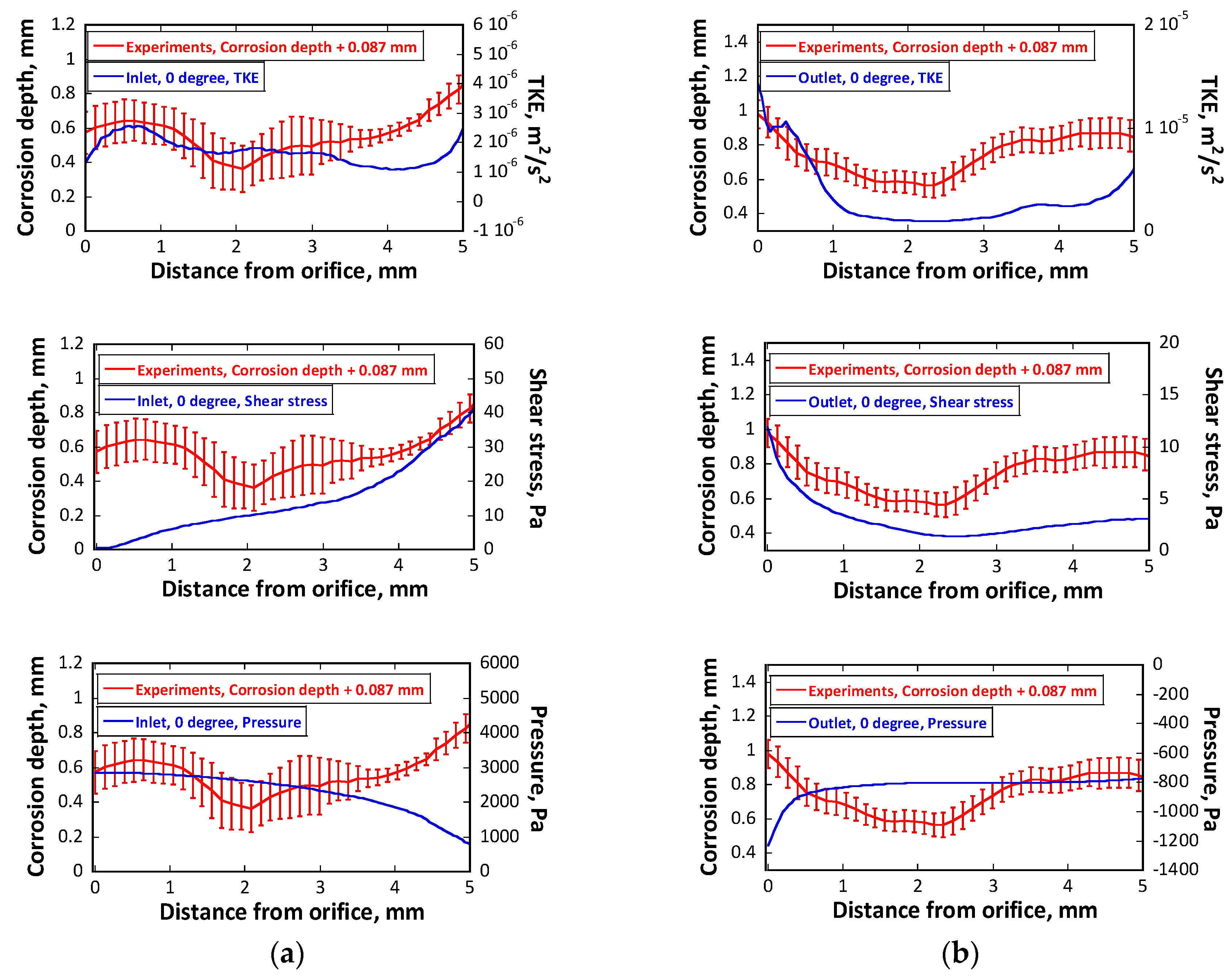
5.2. Effects of the TKE, Shear Stress, and Pressure
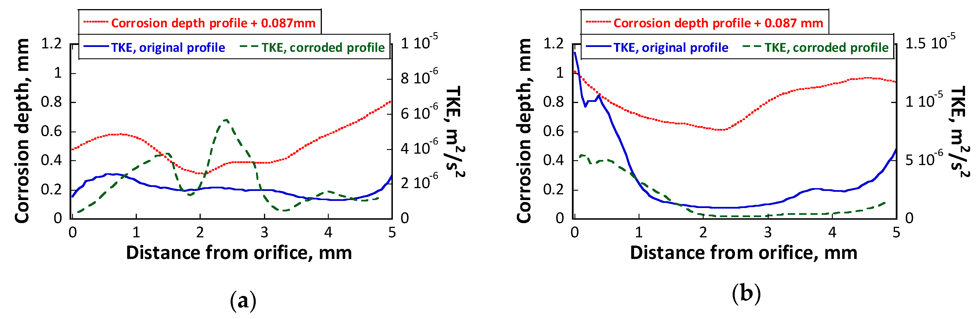
The TKE near the wall, and the shear stress and pressure on the wall along the two orifice surfaces, are plotted in Figure 9 to investigate the effects of different hydrodynamic parameters on the corrosion depth. The average corrosion depths of the two orifices, including a fabrication deviation of 0.087 mm, are also plotted for comparison. Note that the curves obtained from the simulations have been smoothed. It can be seen that the TKE profiles are similar to those of the average corrosion depth of the two orifices, while those for shear stress and pressure are substantially different.
The maximum shear stress on the inlet and outlet orifice walls are low, approximately 40 Pa and 12 Pa, respectively. A study of copper–nickel alloys in sea water has shown that a shear stress of nearly 4650 Pa is insufficient to remove even the surface oxide film [42]. As pointed out previously, no oxygen film formed on the base metal in this study because of the low oxygen concentration in LBE. Furthermore, the critical shear stress capable of mechanically damaging the base metal is much larger than that able to peel off the oxide film. Therefore, it is considered that shear stress is not the main factor leading to FAC herein. Although the pressure fluctuation on the wall in a disturbed flow imposes shear stress on the wall and perhaps causes damage [43], the results obtained under the LBE flow conditions considered here cannot support this assumption because the complex orifice corrosion depth profiles cannot be explained well by monotonic pressure variation along the orifice wall. Rather, it is the variation in the turbulence level near the wall that best explains the corrosion profiles of the orifices.
5.3. Other Effects
5.3.1. Cavitation
It is well known that the passage of fluid through an orifice leads to a sudden large pressure drop downstream, potentially decreasing the pressure below the saturated vapor pressure. As a result, the liquid may rupture and form cavitation bubbles. The subsequent collapses of the cavitation bubbles release microjets and/or shock waves at the wall, causing cavitation damage [44] that can give the wall a rough morphology. The cavitation number, which is used to judge the inception of cavitation in a liquid, is calculated by
where is the cavitation number, is the local pressure, is the vapor pressure of the liquid, is the density of the liquid, and is the characteristic flow speed of the liquid.
Under the present flow conditions, a pressure drop to about −3.58 kPa is generated downstream of the inlet orifice. The vapor pressure of LBE at 450 °C is 3.49 × 10⁻⁴ Pa [38], resulting in a cavitation number of approximately 0.19. It has been reported that the inception cavitation number is about 0.7 for PbBi-68 liquid flow with a Reynolds number in the range 5.8–7.4 × 10⁴ [45]. As the Reynolds number in this study is near this range, a similar inception cavitation number can be applied, indicating that cavitation damage is unlikely to have occurred. Thus, the rough profiles of the orifices can be attributed solely to corrosion damage.
5.3.2. Gravity
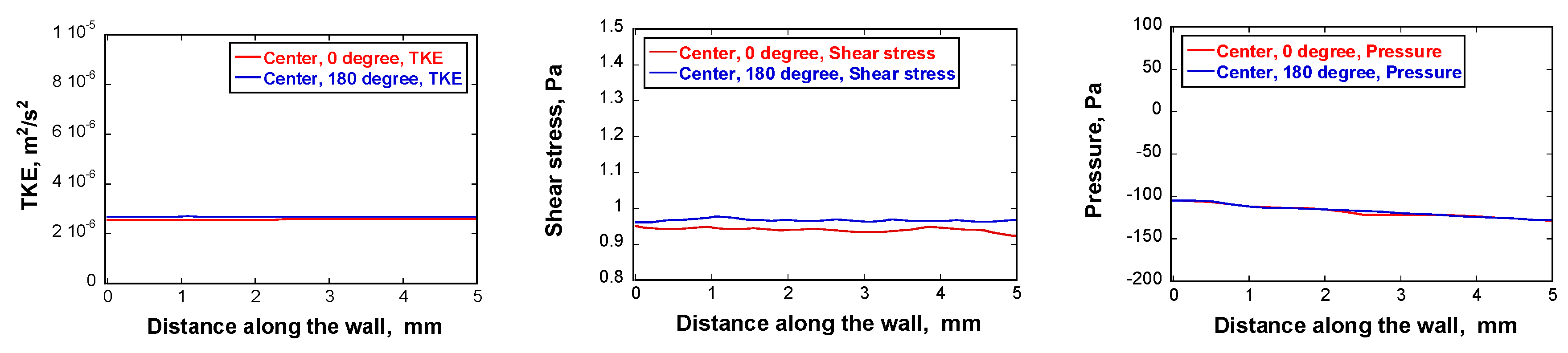
LBE is a high-density liquid metal, so it is necessary to consider the effects of gravity on flow. First, the direction of gravity was set to be perpendicular to the test tube. Figure 10 shows the effects of gravity on various hydrodynamic parameters. The values of 0 and 180 degrees represent the anti-gravity direction and the gravity direction, respectively. The profiles of the hydrodynamic parameters are almost the same at the two circumferential angles, and only tiny differences in the amplitude can be observed.
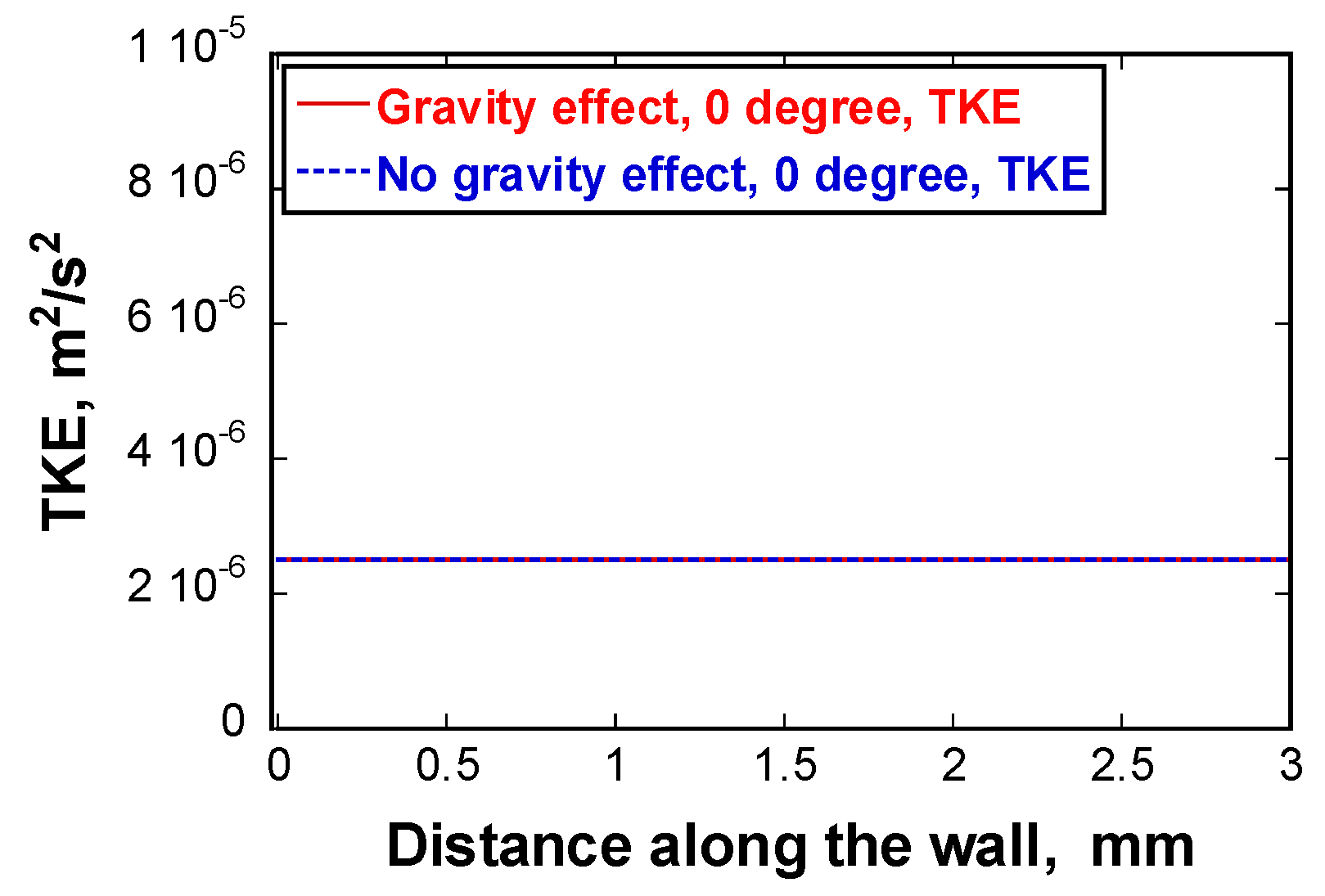
Secondly, gravity was set to be in the direction of the test tube, representing no gravity effect on the flow. Figure 11 shows a comparison of the TKE along the straight central part of the test tube with and without gravity effects. It is hard to distinguish any difference in the TKE profiles. The above results illustrate that the hydrodynamic parameters are insensitive to gravity. This may be because the Reynolds number is high so the strong effect of the inertial force on the flow makes the effects of gravity negligible.
5.3.3. Corroded Morphology
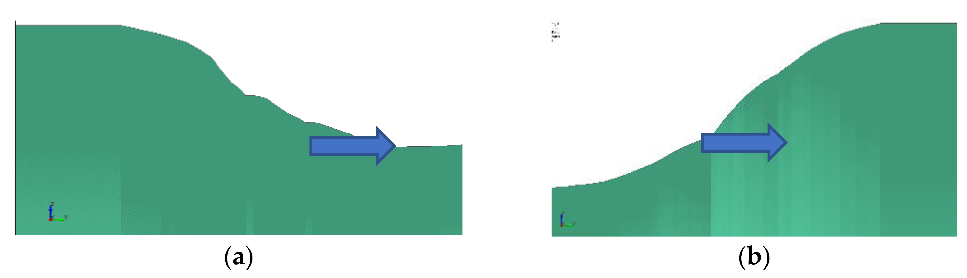
Accumulation of corrosion damage on the inner surface of the wall changes its morphology. A corroded surface could be expected to disturb the flow pattern near the wall, and therefore, the TKE in the near-wall region. To investigate such effects, the experimental corroded surfaces of the two orifices were merged into the simulation models. Figure 12 shows a schematic of the corroded surface profiles used in the simulation, which are the same as the corroded depth profiles at 90 degrees in the experiments. To connect the two orifice parts and the straight central part smoothly, the straight part of the specimen was also assumed to be corroded to a uniform depth of 0.65 mm, which represents an increase in the inner diameter of the straight part of the specimen by 1.3 mm.
Figure 13 plots the TKE for a smooth versus a corroded orifice with distance along the orifice surface. For the inlet orifice, the TKE profile shows much more variability and reaches a considerably higher maximum value in the corroded profile than along the original smooth surface. The peaks in TKE usually appear downstream of sudden protuberances on the corroded surface. This is easy to understand because such convexity enhances the local turbulence level [46]. Interestingly, for the outlet orifice, the magnitude of TKE is relatively weaker for the corroded morphology than with a smooth surface. Furthermore, differences in TKE in the central section are insignificant. This can be attributed to two factors: (1) the corroded outlet orifice surface has fewer protuberances than the corroded inlet orifice surface (Figure 12), so the turbulence level is not locally enhanced; (2) the connections between the straight pipe and the corroded outlet orifice are much smoother than the original ones, which seems to ease the recirculation near the outlet orifice, and therefore, the TKE amplitude.
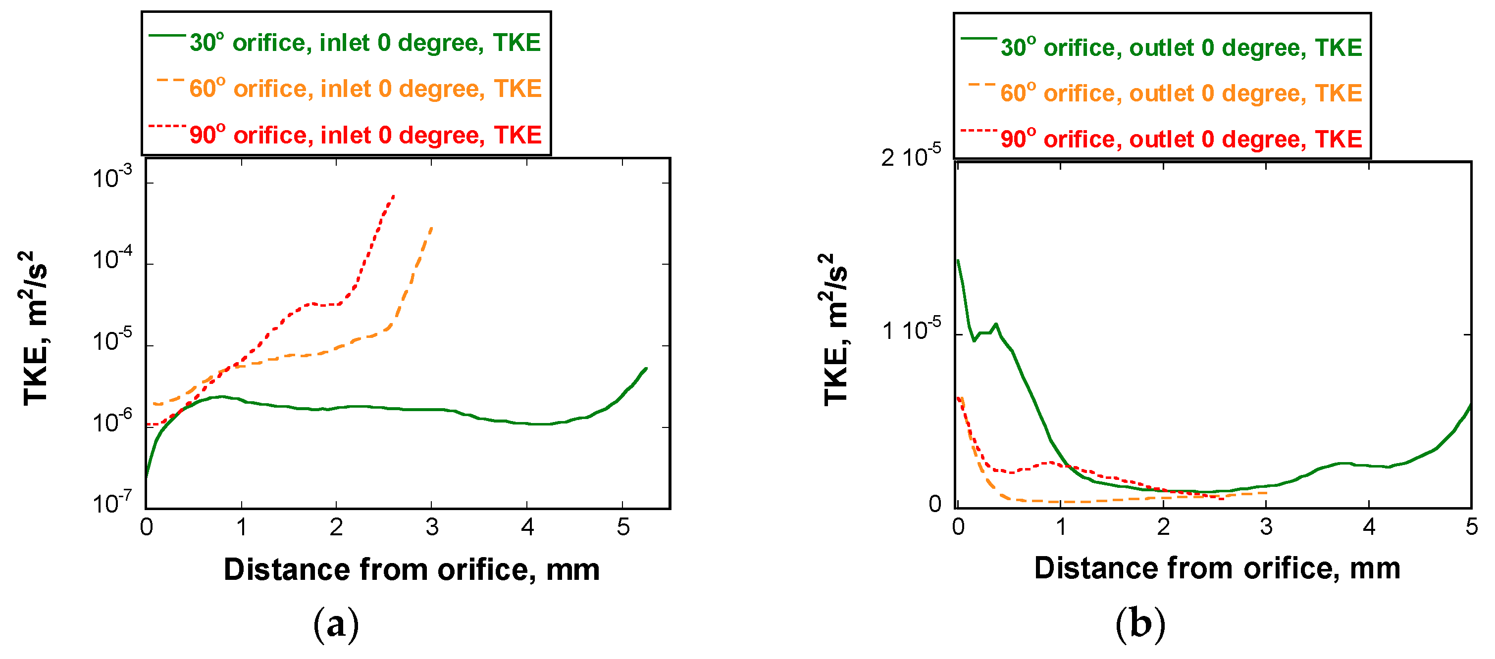
5.3.4. Orifice Angle
The angle of the orifices was altered, from 30 degrees to 60 degrees and 90 degrees, to investigate the effect of orifice angle on flow behavior. This is shown schematically for the inlet orifices in Figure 14, and its effect on TKE is shown in Figure 15. For the outlet orifice, there is no significant difference in the amplitude of TKE. Shan et al. [47] pointed out that the flow field in the recirculation region is insensitive to the ratio between the orifice and pipe diameters. Therefore, it is deduced that the TKE of flow in the recirculation region close to the outlet orifice wall is insensitive to the orifice angle as well. However, for the inlet orifice, the turbulence level is very dependent on the orifice angle. The value for TKE can grow up to several magnitudes higher if the orifice angle changes from 30 to 90 degrees. As TKE has been inferred to significantly influence corrosion depth, extensive corrosion can be anticipated in the 90-degree case. These results provide guidance for system design with flowing LBE—structures with sudden geometry changes should be avoided as much as possible.
5.4. Mass Transfer
5.4.1. Effective Viscosity and Effective Diffusivity
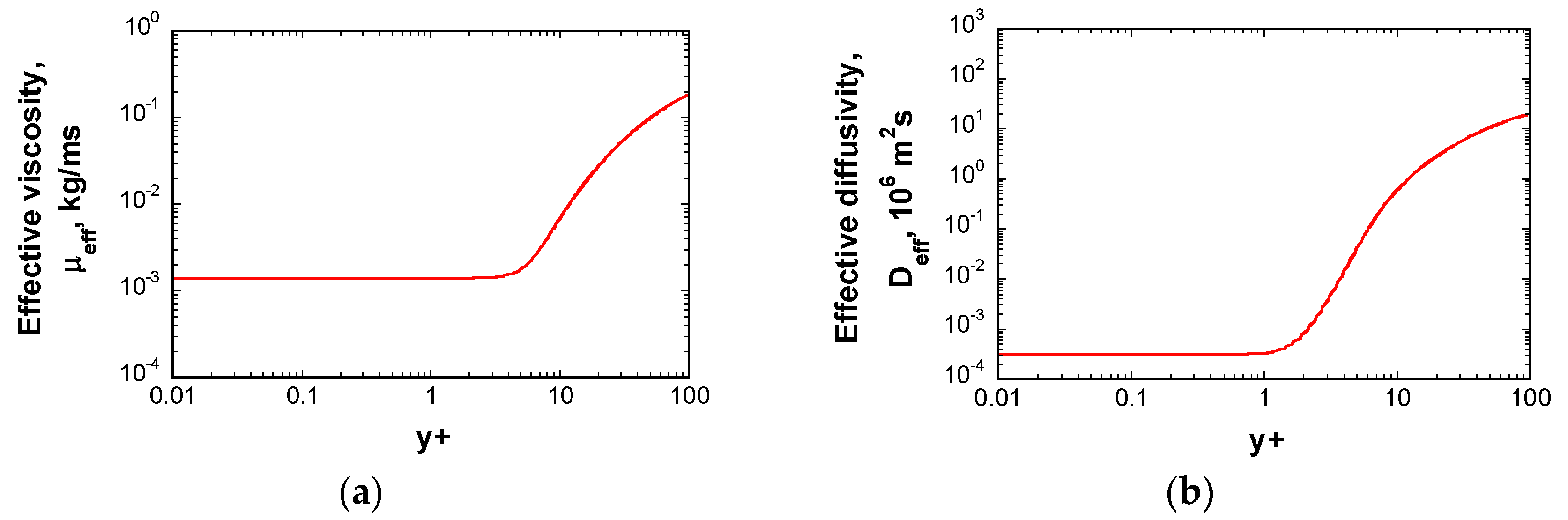
Figure 16 shows the effective viscosity () and effective diffusivity () of iron upstream of the reattachment point. As expected, the effective viscosity remains constant below y+ = 2, which corresponds to the viscous sublayer in the near-wall region. Beyond the viscous sublayer, the turbulent viscosity is much larger than the molecular viscosity, so the turbulent-induced momentum transfer is dominant in species transfer. With approach to the wall, the turbulence level damps rapidly in the viscous sublayer and the turbulent viscosity decreases sharply to a negligible value, indicating that turbulent momentum transfer will, likewise, become insignificant. In the viscous sublayer, however, the effective diffusivity is much larger than the molecular diffusivity; in other words, even weak turbulence can strongly affect species transfer through diffusion [27]. Only when the distance from the wall reaches approximately y+ = 0.4 can the turbulent diffusivity be ignored and the molecular diffusivity be considered dominant in species diffusion. This is in the thin diffusion boundary layer hidden in the viscous sublayer. The relationship between the thickness of the diffusion boundary layer, , and that of the viscous sublayer, , is close to that recommended by Nesic et al. [7]:
5.4.2. Mass Concentration Difference Close to the Wall
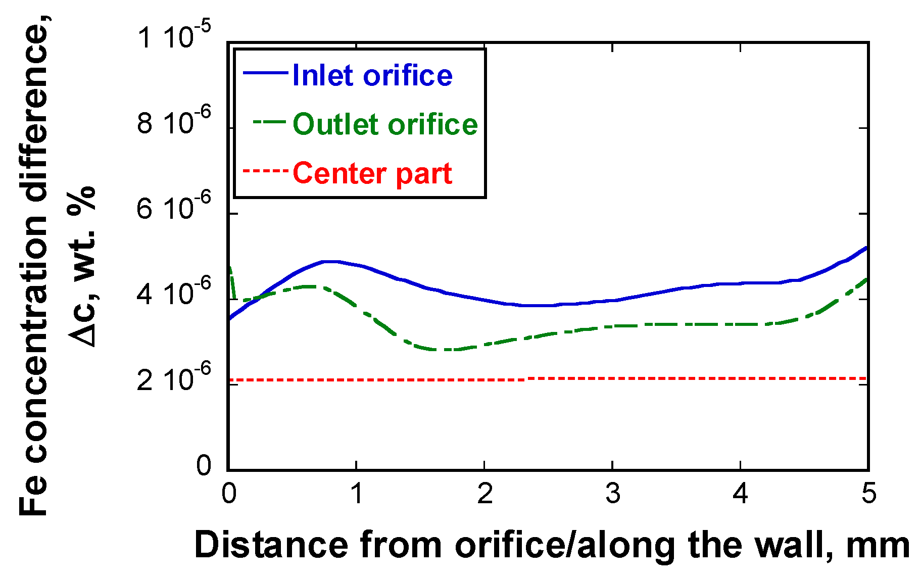
Figure 17 shows the difference in the mass concentration of iron at different locations. This is defined as
In the straight central section of the pipe, the profile is relatively uniform. In comparison, the profiles of at the inlet and outlet orifices are strongly influenced by the turbulent flow. Furthermore, is lower at the outlet orifice than at the inlet orifice. This contrasts with the corrosion depth, which, as shown in Figure 8, is larger at the outlet orifice than the inlet orifice. This may be because the mass transfer coefficient is closely related to the magnitude of roughness [46,48]. Corrosion can be expected to render the smooth wall rough, and perhaps there are differences in the amplitudes of the roughness at the two orifices, resulting in different mass transfer coefficients, and thus, corrosion depths. Prediction of the corrosion depth on the basis of will be considered in the next subsection.
To clarify the correlation between turbulent flow and the mass concentration difference, the profiles of and TKE are plotted together for comparison in Figure 18. Clearly, the profile of is highly coincident with that of TKE near the wall. Therefore, the mass concentration difference can be inferred to be significantly affected by the turbulence level. As shown by Equation (9), the corrosion rate is proportional to , so it can be deduced that the turbulence level can impose direct effects on the corrosion rate of metal.
5.4.3. Comparison of Predicted Corrosion Depth and Measured Corrosion Depth
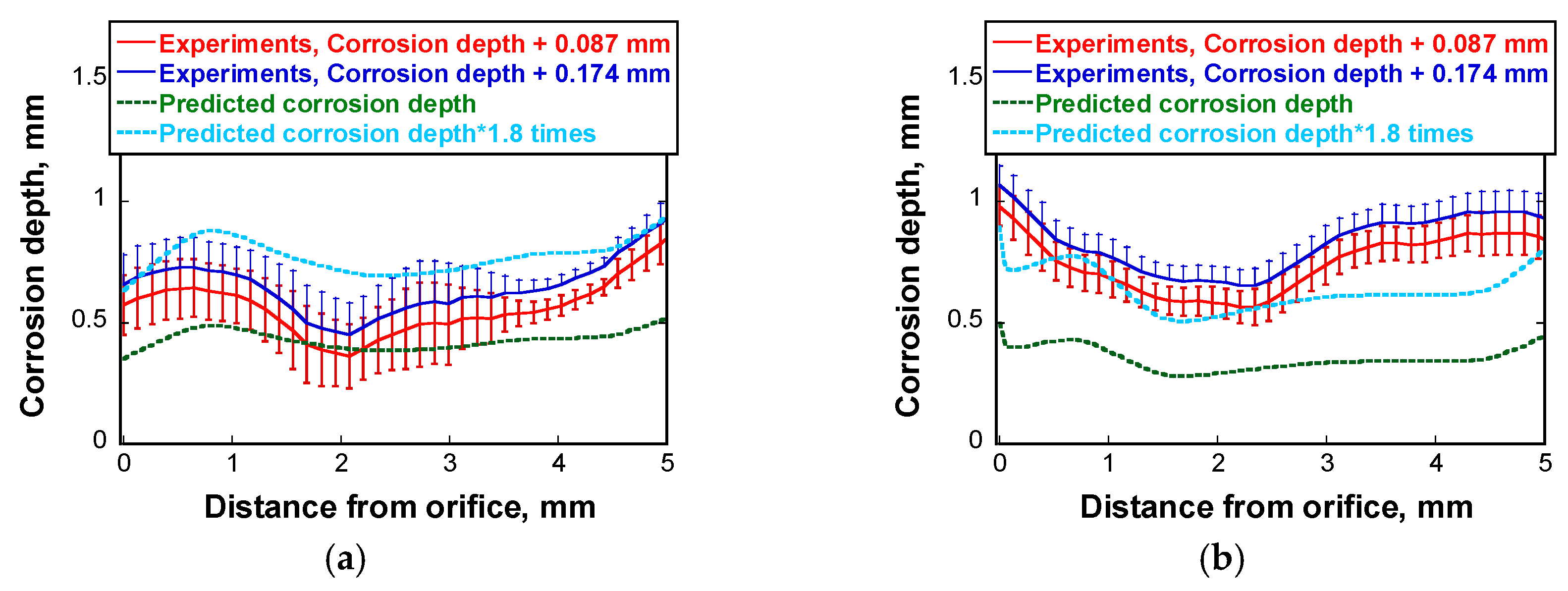
Figure 19 shows a comparison of the predicted corrosion depths calculated with Equation (9) by using the mass concentration differences and the corrosion depths measured from the OM images for the two orifices. The fabrication deviations of 0.087 mm and 0.174 mm are added in the experimental average corrosion depth. The magnitude of the predicted corrosion depth at the inlet orifice is slightly less than the measured corrosion depth with a deviation of 0.087 mm. Moreover, the predicted damage depth at the outlet orifice is much lower than the experimental value. One possible explanation for this is that, as pointed out previously, the effects of wall roughness should be involved, and the different wall roughness values of the inlet and outlet orifices result in different wall mass transfer coefficients; however, exact data on wall roughness is lacking in this study. As an alternative, the calculated corrosion depths of the inlet and outlet orifice were multiplied by a uniform scaler of 1.8 to take wall roughness effects into consideration [7,48]. After multiplying the scaling factor, the magnitudes of the predicted and the measured corrosion depths of the outlet orifice show good coincidence; however, the magnitude of the predicted corrosion depth is slightly higher than the measured corrosion depth, including a deviation of 0.174 mm, which indicates that a scaler less than 1.8 would be applied to the inlet orifice and illustrates that the wall roughness of the inlet orifice is different from that of the outlet orifice. In spite of the arresting coincidence, minor discrepancies can still be observed between the predicted and measured corrosion depth profiles. These may arise for two main reasons: (1) the numerical results are obtained from a model with a smooth surface, while in the experiments, the morphology of the orifice surfaces will have been reshaped gradually by the accumulation of corrosion, and accordingly the turbulence level, and thus, the mass transfer profile will have changed; (2) the wall roughness along the orifice surfaces may be non-uniform. Nevertheless, the results indicate that the turbulence level in the near-wall region has a strong influence on the corrosion depth profile. Furthermore, the corrosion depth can be predicted successfully by calculating the mass transfer coefficient by integrating the corrosion model into the turbulent flow model.
Researchers in Italy have studied the corrosion of cylindrical AISI 316L SS samples using the LECOR loop. The experiment was performed for 1500 h under the same temperature difference and similar oxygen concentration conditions as are used in this study [49]. They reported an average corrosion rate of 1.9 × 10⁻³ µm/h, which is one magnitude lower than that for the straight central part of the current study’s experiment where flow has fully developed. This difference may result from the combined effects of three factors: (1) the absolute temperature is higher in the present study, so the solubility and diffusion coefficient of iron in LBE are higher; (2) the Reynolds number in the LECOR loop is about one-fifth of that in the present study, making the diffusion boundary layer is much thicker, and therefore, mass transfer resistance is much stronger. It has been pointed out that has a nearly linear correlation with for roughened wall surfaces [48,50]; (3) the dimensionless wall roughness in the LECOR loop is much lower than that of the present study, and it is also known that the mass transfer coefficient depends on the dimensionless wall roughness [48]. The predicted depth of corrosion in the straight section of the pipe after 3000 h of operation is about 0.21 mm, which is about 1.3–3.5 times the average experimental corrosion depth (0.06–0.16 mm); this ratio is similar to that reported in another study [51]. Overestimation of the corrosion rate in the simulation may result from [51,52]: (1) the diffusion coefficient of iron in liquid LBE at 450 °C not being known sufficiently precisely; (2) the assumption that the liquid metal is saturated at the solid/liquid interface.
Furthermore, the absolute corrosion depth of the specimen is extremely high in the present experiment, which would not be acceptable for real engineering applications. For example, one of the future ADS concepts proposed by JAEA is an LBE spallation target that requires a significant contraction of the LBE flow path at the beam window [53]. The Reynolds number at the beam window is much higher than that of the present study, and the beam window would be required to survive extreme service conditions [54]. Moreover, considering the poor wettability of LBE to 316L SS, the corrosion depth could be larger because slip at the solid/liquid boundary enhances the turbulence level in the near-wall region [55]. In addition, it is known that the structural steel will withstand strong irradiation during its service period, and it has been also reported that the cold-worked steel experiences different corrosion behaviors than the solution-annealed steel in LBE under static and flow LBE conditions, which can be attributed to the alteration of the dominant corrosion process [56,57]. It has also been pointed out that the effects of steel microstructure on FAC depend on the relative thickness between the selective corrosion layer in the solid and the diffusion boundary layer in the fluid. If the former is thicker, the microstructure effects can be visible; otherwise, it can be ignored [30]. Nevertheless, the effects of microstructure on FAC under LBE flowing condition requires thorough and systematical investigation in the future.
Those above-combined factors mean that it is extremely important to devise ways to increase the mass transfer resistance between the base metal and the LBE. Several studies have indicated that the formation of a protective oxide layer can greatly decrease the corrosion rate of 316L SS in static LBE [58,59]. Controlling the oxygen concentration in LBE to a specific range is critical to form an effective self-healing oxide film, and meanwhile avoid the deposition of uncalled-for oxide products (e.g., PbO) on the cold legs, potentially causing blockage [39].
For future ADSs that adopt LBE as the coolant material, even once an effective protective oxide film has formed on the structural material, it may be broken or thinned by turbulence pounding [6] and various stresses. These include not only the shear stress resulting from turbulent flow, but the thermal stress caused by pulsed proton beam injections and fatigue stress from thermal shocks. Such stresses are generally very large, and their effects on oxide film should be investigated in detail. The effects of absolute temperature and temperature difference on corrosion behavior should also be investigated.
6. Conclusions
FAC behavior of 316L SS under LBE turbulent flow was studied by using the JLBL-1 loop under non-isothermal conditions, and CFD analyses were performed to study the associated hydromechanics and mass transfer. It was found that corrosion of the 316L SS is very severe. Corrosion can reach a maximum depth of approximately 10% of the tube wall thickness in the straight part of the specimen pipe, where the flow is fully developed. However, this ratio increases by as much as 50% at the inlet and outlet orifices, where abrupt changes in the diameter of the specimen lead to changes in the flow direction and/or recirculation. The corrosion profile is correlated with the near-wall turbulence level, but does not seem to correlate with the local shear stress and pressure profiles. In addition, morphological changes during the corrosion process influence the near-wall turbulence level. Moreover, it is shown that the near-wall turbulence level is extremely sensitive to the orifice angle, and that right-angled orifices should be avoided to suppress FAC.
Mass transfer analysis shows that the local turbulence level determines the mass concentration distribution in the near-wall region, thus significantly affecting the mass transfer coefficient. As a consequence, the mass transfer is an effective means of predicting the depth of FAC, which can be calculated with the assistance of CFD analyses with a corrosion model. The corrosion depth was calculated on the basis of the mass transfer coefficient obtained in the numerical simulation and was compared with that obtained in the loop. For the inlet orifice part, the predicted corrosion depth is comparable with the measured corrosion depth; for the outlet orifice part, the predicted corrosion depth is less than the measured corrosion depth, however, this gap was filled well after taking the wall roughness effects into consideration; for the straight tube part, the predicted corrosion depth is larger than the average experimental corrosion depth, which perhaps can be attributed to the fact that the iron concentration on the wall did not reach its saturation value, as assumed. Considering that many other factors beyond the range of the present study can lead to much more severe FAC, formation of an oxide layer is an extremely important means of preventing the rapid development of FAC. In the future, research on corrosion behavior under precisely controlled oxygen, flow speed, and temperature conditions will be carried out.
Author Contributions
T.W. carried out the numerical simulations; S.S. performed the experiments; T.W. analyzed the data; T.W. and S.S. were responsible for writing the paper.
Funding
This research received no external funding.
Acknowledgments
The first author sincerely appreciates Masatoshi Futakawa of J-PARC Center, JAEA, for providing valuable comments and discussions. The authors also extend their thanks to Hironari Obayashi and Toshinobu Sasa of J-PARC Center, JAEA, for useful and interesting discussions.
Conflicts of Interest
The authors declare no conflict of interest.
Nomenclature
| constants in empirical equations linking to and | |
| cavitation number | |
| , , | species concentration in the bulk fluid, at the wall, and in the first node, kmol/m3 |
| oxygen concentration in a liquid, kmol/m3 | |
| hydraulic diameter, m | |
| molecular diffusion coefficient, m2/s | |
| eddy or turbulent diffusivity, , m2/s | |
| effective diffusion coefficient, , m2/s | |
| , | damping factor in the LRN turbulence model |
| turbulence level in the near-wall region | |
| mass flux of iron, | |
| turbulent kinetic energy, m2/s2 | |
| mass transfer coefficient, m/s | |
| chemical component of a material | |
| molar mass of iron, kg/kmol | |
| generation of turbulence, | |
| additional term of turbulence generation in the LRN turbulence model, | |
| local pressure in a liquid, Pa | |
| vapor pressure of a liquid, Pa | |
| wall roughness, m | |
| Reynolds number, | |
| , | turbulence Reynolds number, , |
| Schmidt number, | |
| turbulent Schmidt number, | |
| Sherwood number, | |
| temperature, K | |
| temperature difference, K | |
| dimensionless velocity | |
| characteristic flow speed of a liquid, m/s | |
| distance from the wall, m | |
| dimensionless distance from the wall | |
| distance of the first node from the wall, m | |
| Greek symbols | |
| thickness of diffusion boundary layer, m | |
| thickness of viscous sublayer, m | |
| dissipation of turbulent kinetic energy, m2/s3 | |
| molecular dynamic viscosity, | |
| eddy or turbulent viscosity, | |
| effective viscosity, , | |
| density, | |
| wall shear stress, Pa |
References
- Bergman, T.L.; Incropera, F.P.; Devitt, D.P.; Lavine, A.S. Fundamentals of Heat and Mass Transfer, 7th ed.; John Wiley & Sons: Hoboken, NJ, USA, 2011; pp. 378–418. [Google Scholar]
- Mahato, B.K.; Voora, S.K.; Schemilt, L.W. Steel pipe corrosion under flow conditions—I. an isothermal correlation for a mass transfer model. Corros. Sci. 1968, 8, 173–193. [Google Scholar] [CrossRef]
- Corpson, H.R. Effects of velocity on corrosion. Corrosion 1960, 16, 130–136. [Google Scholar]
- Silverman, D.C. Rotating cylinder electrode for velocity sensitivity testing. Corrosion 1984, 40, 220–226. [Google Scholar] [CrossRef]
- Silverman, D.C. Rotating cylinder electrode—Geometry relationships for prediction of velocity-sensitive corrosion. Corrosion 1987, 44, 42–49. [Google Scholar] [CrossRef]
- Nesic, S.; Postlethwaite, J. Relationship between the structure of disturbed flow and erosion-corrosion. Corrosion 1990, 46, 874–880. [Google Scholar] [CrossRef]
- Nesic, S.; Postlethwaite, J. Hydrodynamics of disturbed flow and erosion-corrosion. Part I—Single-phase flow study. Can. J. Chem. Eng. 1991, 69, 698–703. [Google Scholar] [CrossRef]
- Mahato, B.K.; Cha, C.Y.; Shemilt, L.W. Unsteady state mass transfer coefficients controlling steel pipe corrosion under isothermal flow conditions. Corros. Sci. 1980, 20, 421–441. [Google Scholar] [CrossRef]
- Chang, Y.S.; Kim, S.H.; Chang, H.S.; Lee, S.M.; Choi, J.B.; Kim, Y.J.; Choi, Y.H. Fluid effects on structural integrity of pipes with an orifice and elbows with a wall-thinned part. J. Loss Prev. Proc. 2009, 22, 854–859. [Google Scholar] [CrossRef]
- Utanohara, Y.; Nagaya, Y.; Nakamura, A.; Murase, M. Influence of local flow field on flow accelerated corrosion downstream from an orifice. J. Power Energy Syst. 2012, 6, 18–33. [Google Scholar] [CrossRef]
- Utanohara, Y.; Nagaya, Y.; Nakamura, A.; Murase, M.; Kamahori, K. Correlation between flow accelerated corrosion and wall shear stress downstream from an orifice. J. Power Energy Syst. 2013, 7, 138–146. [Google Scholar] [CrossRef]
- Crawford, N.M.; Cunningham, G.; Spence, S.W.T. An experimental investigation into the pressure drop for turbulent flow in 90° elbow bends. Proc. Inst. Mech. Eng. Part E J. Process Mech. Eng. 2007, 221, 77–88. [Google Scholar] [CrossRef]
- Nesic, S. Using computational fluid dynamics in combating erosion-corrosion. Chem. Eng. Sci. 2006, 61, 4086–4097. [Google Scholar] [CrossRef]
- Poulson, B. Complexities in predicting erosion corrosion. Wear 1999, 233–235, 497–504. [Google Scholar] [CrossRef]
- El-Gammal, M.; Mazhar, H.; Cotton, J.S.; Shefski, C.; Pietralik, J.; Ching, C.Y. The hydrodynamic effects of single-phase flow on flow accelerated corrosion in a 90-degree elbow. Nucl. Eng. Des. 2010, 240, 1589–1598. [Google Scholar] [CrossRef]
- El-Gammal, M.; Ahmed, W.H.; Ching, C.Y. Investigation of wall mass transfer characteristics downstream of an orifice. Nucl. Eng. Des. 2012, 242, 353–360. [Google Scholar] [CrossRef]
- Takano, T.; Ikarashi, Y.; Uchiyama, K.; Yamagata, T.; Fujisawa, N. Influence of swirling flow on mass and momentum transfer downstream of a pipe with elbow and orifice. Int. J. Heat Mass Transf. 2016, 92, 394–402. [Google Scholar] [CrossRef]
- Ikarashi, Y.; Taguchi, S.; Yamagata, T.; Fujisawa, N. Mass and momentum transfer characteristics in and downstream of 90° elbow. Int. J. Heat Mass Transf. 2017, 107, 1085–1093. [Google Scholar] [CrossRef]
- Gromov, B.F.; Belomitcev, Y.S.; Yefimov, E.I.; Leonchuk, M.P.; Martinov, P.N.; Orlov, Y.I.; Pankratov, D.V.; Pashkin, Y.G.; Toshinsky, G.I.; Chekunov, V.V.; et al. Use of lead-bismuth coolant in nuclear reactors and accelerator-driven systems. Nucl. Eng. Des. 1997, 173, 207–217. [Google Scholar] [CrossRef]
- Zhang, J. Lead-Bismuth Eutectic (LBE): A coolant candidate for Gen. IV advanced nuclear reactor concepts. Adv. Eng. Mater. 2014, 16, 349–356. [Google Scholar] [CrossRef]
- Zhang, J. A review of steel corrosion by liquid lead and lead-bismuth. Corros. Sci. 2009, 51, 1207–1227. [Google Scholar] [CrossRef]
- Zhang, J.; Hoseman, P.; Maloy, S. Models of liquid metal corrosion. J. Nucl. Mater. 2010, 404, 82–96. [Google Scholar] [CrossRef]
- Zhang, J.; Li, N. Review of the studies on fundamental issues in LBE corrosion. J. Nucl. Mater. 2008, 373, 351–377. [Google Scholar] [CrossRef]
- Schroer, C.; Wedemeyer, O.; Novotny, J.; Skrypnik, A.; Konys, J. Long-term service of austenitic steel 1.4571 as a container material for flowing lead–bismuth eutectic. J. Nucl. Mater. 2011, 418, 8–15. [Google Scholar] [CrossRef]
- STAR-CD methodology, Ver. 4.26; Siemens Product Lifecycle Management Inc.: Plano, TX, USA, 2016.
- Launder, B.E.; Spalding, D.B. The numerical computation of turbulent flows. Comp. Meth. Appl. Mech. Eng. 1974, 3, 269–289. [Google Scholar] [CrossRef]
- Nesic, S.; Postlethwaite, J. Calculation of wall-mass transfer rates in separated aqueous flow using a low Reynolds number k − ε model. Int. J. Heat Mass Transf. 1992, 35, 1977–1985. [Google Scholar] [CrossRef]
- Lien, F.S.; Chen, W.L.; Leschziner, M.A. Low-Reynolds-Number Eddy-Viscosity Modelling Based on Non-Linear Stress-Strain/Vorticity Relations. In Proceedings of the 3rd Symposium on Engineering Turbulence Modelling and Measurements, Crete, Greece, 27–29 May 1996. [Google Scholar]
- He, X.; Li, N.; Mineev, M. A kinetic model for corrosion and precipitation in non-isothermal LBE flow loop. J. Nucl. Mater. 2001, 297, 214–219. [Google Scholar] [CrossRef]
- Simon, N.; Terlain, A.; Flament, T. The compatibility of austenitic materials with liquid Pb-17Li. Corros. Sci. 2001, 43, 1041–1052. [Google Scholar] [CrossRef]
- Yamaki, E.; Ginestar, K.; Martinelli, L. Dissolution mechanism of 316L in lead-bismuth eutectic at 500 °C. Corros. Sci. 2011, 53, 3075–3085. [Google Scholar] [CrossRef]
- Schad, M. To the corrosion of austenitic steel in sodium loops. Nucl. Tech. 1980, 50, 267–288. [Google Scholar] [CrossRef]
- Distefano, J.R.; Hoffman, E.E. Corrosion Mechanisms in Refractory Metal-Alkali Metal Systems. At. Energy Rev. 1964, 2, 3–33. [Google Scholar]
- Keating, A. A Model for the Investigation of Two-Phase Erosion-Corrosion in Complex Geometries. Maters’s Thesis, University of Queensland, Brisbane, QLD, Australia, 1999. [Google Scholar]
- Davis, C.; Frawley, P. Modelling of erosion-corrosion in practical geometries. Corros. Sci. 2009, 51, 769–775. [Google Scholar] [CrossRef]
- Kikuchi, K.; Karata, Y.; Saito, S.; Fukazawa, M.; Salsa, T.; Okinawa, H.; Wake, E.; Miura, K. Corrosion–erosion test of SS316 in flowing Pb–Bi. J. Nucl. Mater. 2003, 318, 348–354. [Google Scholar] [CrossRef]
- Kikuchi, K.; Saito, S.; Kurata, Y.; Futakawa, M.; Sasa, T.; Oigawa, H.; Wakai, E.; Umeno, M.; Mizubayashi, H.; Miura, K. Lead-bismuth eutectic compatibility with materials in the concept of spallation target for ADS. JSME Int. J. B-Fluid Therm. 2004, 47, 332–339. [Google Scholar] [CrossRef]
- OECD NEA. Handbook on Lead-Bismuth Eutectic Alloy and Lead Properties, Materials Compatibility, Thermal-Hydraulics and Technologies; 2015 Edition; OECD NEA: Boulogne-Billancourt, France, 2015. [Google Scholar]
- Li, N. Active control of oxygen in molten lead–bismuth eutectic systems to prevent steel corrosion and coolant contamination. J. Nucl. Mater. 2002, 300, 73–81. [Google Scholar] [CrossRef]
- Balbaud-Celerier, F.; Barbier, F. Influence of the Pb-Bi hydrodynamics on the corrosion of T91 martensitic steel and pure iron. J. Nucl. Mater. 2004, 335, 204–209. [Google Scholar] [CrossRef]
- Abella, J.; Verdaguer, A.; Colominas, S.; Ginestar, K.; Martinelli, L. Fundamental data: Solubility of nickel and oxygen and diffusivity of iron and oxygen in molten LBE. J. Nucl. Mater. 2011, 415, 329–337. [Google Scholar] [CrossRef]
- Syrett, B.C. Erosion-corrosion of copper-nickel alloys in sea water and other aqueous environments—A literature review. Corrosion 1976, 32, 242–252. [Google Scholar] [CrossRef]
- Heitz, E. Chemo-mechanical effects of flow on corrosion. Corrosion 1991, 47, 135–145. [Google Scholar] [CrossRef]
- Brennen, C.E. Cavitation and Bubble Dynamics; Oxford University Press: Oxford, UK, 1995. [Google Scholar]
- Yada, H.; Kanagawa, A.; Hattori, S. Cavitation inception and erosion in flowing system of water and liquid metal. Trans. Jpn. Soc. Mech. Eng. Ser. B 2011, 78, 811–820. (In Japanese) [Google Scholar] [CrossRef]
- Fujisawa, N.; Uchiyama, K.; Yamagata, T. Mass transfer measurements on periodic roughness in a circular pipe and downstream of orifice. Int. J. Heat Mass Transf. 2017, 105, 316–325. [Google Scholar] [CrossRef]
- Shan, F.; Liu, Z.; Liu, W.; Tsuji, Y. Effects of the orifice to pipe diameter ratio on orifice flows. Chem. Eng. Sci. 2016, 152, 497–506. [Google Scholar] [CrossRef]
- Postlethwaite, J.; Lotz, U. Mass transfer at erosion-corrosion roughened surfaces. Can. J. Chem. Eng. 1988, 66, 75–78. [Google Scholar] [CrossRef]
- Fazio, C.; Ricapito, I.; Scaddozzo, G.; Benamati, G. Corrosion behaviour of steels and refractory metals and tensile features of steels exposed to flowing PbBi in the LECOR loop. J. Nucl. Mater. 2003, 318, 325–332. [Google Scholar] [CrossRef]
- Poulson, B. Mass transfer from rough surfaces. Corros. Sci. 1990, 30, 743–746. [Google Scholar] [CrossRef]
- Balbaud-Celerier, F.; Barbier, F. Investigation of models to predict the corrosion of steels in flowing liquid lead alloys. J. Nucl. Mater. 2001, 289, 227–242. [Google Scholar] [CrossRef]
- Malang, S.; Smith, D.L. Modeling of Liquid Metal Corrosion/Deposition in a Fusion Reactor Blanket (No. ANL/FPP/TM-192); Argonne National Lab.: Lemont, IL, USA, 1984.
- Sugawara, T.; Nishihara, K.; Obayashi, H.; Kurata, Y.; Oigawa, H. Conceptual design study of beam window for accelerator-driven system. J. Nucl. Sci. Technol. 2010, 47, 953–962. [Google Scholar] [CrossRef]
- Wan, T.; Naoe, T.; Wakui, T.; Futakawa, M.; Obayashi, H.; Sasa, T. Study on the evaluation of erosion damage by using laser ultrasonic integrated with a wavelet analysis technique. J. Phys. Conf. Ser. 2017, 842, 012010. [Google Scholar] [CrossRef] [Green Version]
- Yoon, M.; Hwang, J.; Lee, J.; Sung, H.J.; Kim, J. Large-scale motions on a turbulent channel flow with the slip boundary condition. Int. J. Heat Mass Transf. 2016, 61, 96–107. [Google Scholar] [CrossRef]
- Rivai, A.K.; Saito, S.; Tezuka, M.; Kato, C.; Kikuchi, K. Effect of cold working on the corrosion resistance of JPCA stainless steel in flowing Pb–Bi at 450 °C. J. Nucl. Mater. 2012, 431, 97–104. [Google Scholar] [CrossRef]
- Lambrinou, K.; Charalampopoulou, E.; Donck, T.V.; Delville, R.; Schryvers, D. Dissolution corrosion of 316L austenitic stainless steels in contact with static liquid lead-bismuth eutectic (LBE) at 500 °C. J. Nucl. Mater. 2017, 490, 9–27. [Google Scholar] [CrossRef]
- Kurata, Y.; Masatoshi, F.; Saito, S. Corrosion behavior of steels in liquid lead–bismuth with low oxygen concentrations. J. Nucl. Mater. 2008, 373, 164–178. [Google Scholar] [CrossRef]
- Kurata, Y. Corrosion experiments and materials developed for the Japanese HLM systems. J. Nucl. Mater. 2011, 415, 254–259. [Google Scholar] [CrossRef]
Figure 1.
Schematic of the boundary layer where turbulent flow meets a no-slip wall boundary.

Figure 2.
Schematic of the effects of turbulent flow on the corrosion rate of the base metal.

Figure 3.
Schematic drawing of steel corrosion in lead–bismuth eutectic (LBE) at low oxygen concentration.
Figure 3.
Schematic drawing of steel corrosion in lead–bismuth eutectic (LBE) at low oxygen concentration.

Figure 4.
Flow diagram of JLBL-1.

Figure 5.
Geometry of specimen tubing.

Figure 6.
Example of a half 3D model used in the numerical simulation.

Figure 7.
OM and SEM images. (a) OM image of cross-sections of the specimen of the central straight pipe; (b) SEM image of cross-section of the specimen of the central straight pipe; (c) OM images of the two orifices at various circumferential angles.
Figure 7.
OM and SEM images. (a) OM image of cross-sections of the specimen of the central straight pipe; (b) SEM image of cross-section of the specimen of the central straight pipe; (c) OM images of the two orifices at various circumferential angles.

Figure 8.
(a,b) Corrosion depth profiles of the inlet and outlet orifices at various circumferential angles as a function of the distance along the orifice surface. Fabrication deviations of 0.087 mm are added in the measured corrosion depth; (c,d) average corrosion depth of inlet orifice and outlet orifice. Fabrication deviations of 0.087 mm and 0.174 mm are added in the measured average corrosion depth, respectively.

Figure 9.
Comparison of the average corrosion depth with the turbulent kinetic energy (TKE) near the wall and the shear stress and pressure on the wall for the two orifices. (a) Inlet orifice; (b) Outlet orifice.
Figure 9.
Comparison of the average corrosion depth with the turbulent kinetic energy (TKE) near the wall and the shear stress and pressure on the wall for the two orifices. (a) Inlet orifice; (b) Outlet orifice.

Figure 10.
Effects of gravity on various hydrodynamic parameters.

Figure 11.
Comparison of TKE along the straight central part of the test tube with and without a gravity effect.
Figure 11.
Comparison of TKE along the straight central part of the test tube with and without a gravity effect.

Figure 12.
Schematic of the corroded surface profiles adopted in the simulations. (a) Inlet orifice; (b) Outlet orifice.
Figure 12.
Schematic of the corroded surface profiles adopted in the simulations. (a) Inlet orifice; (b) Outlet orifice.

Figure 13.
Effects of the corroded surface on TKE in the near-wall region at the two orifices. The utilized corrosion depth profile is plotted together for comparison. (a) Inlet orifice; (b) Outlet orifice.
Figure 13.
Effects of the corroded surface on TKE in the near-wall region at the two orifices. The utilized corrosion depth profile is plotted together for comparison. (a) Inlet orifice; (b) Outlet orifice.

Figure 14.
Schematics of inlet orifices with different angles. Note that only the outlet orifices are not shown.
Figure 14.
Schematics of inlet orifices with different angles. Note that only the outlet orifices are not shown.

Figure 15.
Effects of orifice angle on TKE in the near-wall region for the two orifices. (a) Inlet orifice; (b) Outlet orifice.
Figure 15.
Effects of orifice angle on TKE in the near-wall region for the two orifices. (a) Inlet orifice; (b) Outlet orifice.

Figure 16.
Effective viscosity and effective diffusivity of iron upstream of the reattachment point. (a) Effective viscosity; (b) Effective diffusivity.
Figure 16.
Effective viscosity and effective diffusivity of iron upstream of the reattachment point. (a) Effective viscosity; (b) Effective diffusivity.

Figure 17.
Mass concentration difference of iron at various locations.

Figure 18.
Comparison of mass concentration difference and TKE near the wall. (a) Inlet orifice; (b) Outlet orifice.
Figure 18.
Comparison of mass concentration difference and TKE near the wall. (a) Inlet orifice; (b) Outlet orifice.
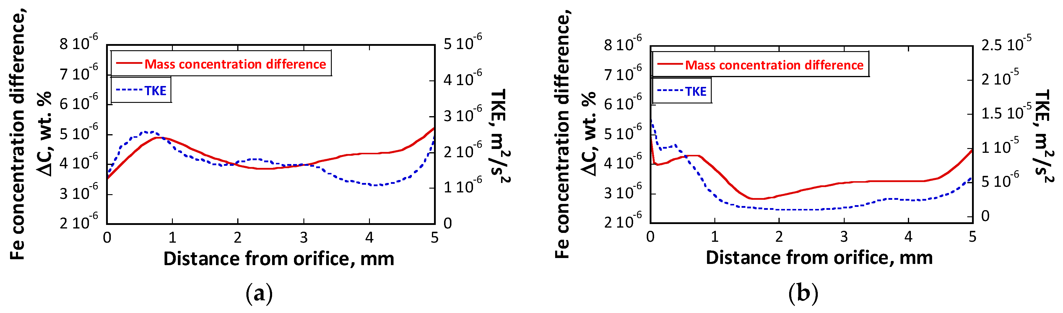
Figure 19.
Comparison of the predicted corrosion depths calculated from Equation (9) using the mass concentration difference and the corrosion depths measured from the OM images at the two orifices. Note that the fabrication deviations of 0.087 mm and 0.174 mm are added in the experimental corrosion depth, respectively, and the predicted corrosion depths of the inlet orifice and outlet orifice were multiplied by a scaler of 1.8 to take the wall roughness into consideration. (a) Inlet orifice; (b) Outlet orifice.

© 2018 by the authors. Licensee MDPI, Basel, Switzerland. This article is an open access article distributed under the terms and conditions of the Creative Commons Attribution (CC BY) license (http://creativecommons.org/licenses/by/4.0/).
Share and Cite
MDPI and ACS Style
Wan, T.; Saito, S. Flow-Accelerated Corrosion of Type 316L Stainless Steel Caused by Turbulent Lead–Bismuth Eutectic Flow. Metals 2018, 8, 627. https://doi.org/10.3390/met8080627
AMA Style
Wan T, Saito S. Flow-Accelerated Corrosion of Type 316L Stainless Steel Caused by Turbulent Lead–Bismuth Eutectic Flow. Metals. 2018; 8(8):627. https://doi.org/10.3390/met8080627
Chicago/Turabian StyleWan, Tao, and Shigeru Saito. 2018. "Flow-Accelerated Corrosion of Type 316L Stainless Steel Caused by Turbulent Lead–Bismuth Eutectic Flow" Metals 8, no. 8: 627. https://doi.org/10.3390/met8080627
Note that from the first issue of 2016, this journal uses article numbers instead of page numbers. See further details here.