The models were developed in ANSYS 5.7. The validity of the model predictions were tested against experimental samples tested to destruction. This section begins by briefly describing the experimental series against which model predictions were compared.
2.1. Experimental
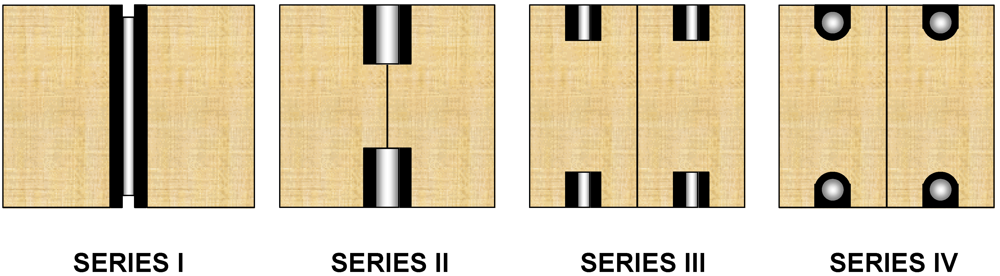
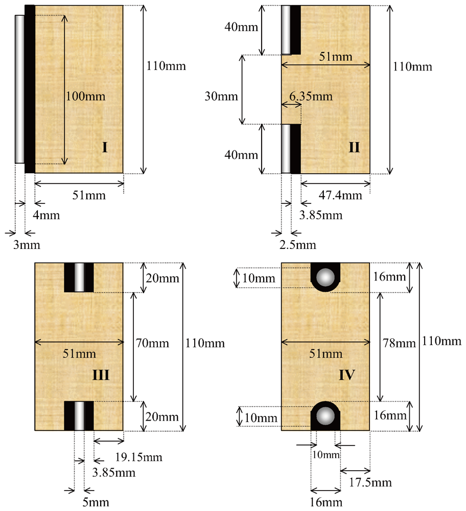
Figure 1 shows the cross sections of four different reinforcement configurations (Series I-IV). Series I composite beams were full depth flitch beams where the reinforcing steel was vertically laminated between two sections of Kerto S laminated veneer lumber (LVL) to a depth of 50 mm either side of the axis of neutrality. Testing carried out at the University of Bath on LVL specimens have shown the mean bending modulus is 12.4 GPa, 50 MPa value for strength, 0.62 GPa value for the shear modulus and a Poisson’s ratio of 0.29. The LVL was cut to 110 mm to avoid geometric instability. Each beam was 1900 mm long. Series II beams were manufactured by bonding together two LVL sections (1900 mm long, 51 mm wide and 110 mm deep). A 40 mm deep and 12.7 mm wide groove was then routed along the centre of the beam axis on both the tensile and compressive faces of the beam. 40 mm deep reinforcements were then slotted and glued into the grooves on either face. Series III beams were, like series II beams, initially bonded together as vertically laminated LVL sections after which grooves were routed into the tensile and compressive faces of the beams but this time at a depth of 20 mm and a width of 12.7 mm, with two grooves routed into each face in the centre and along the axis of each LVL segment. 20 mm deep reinforcing plates were then slotted and glued into the grooves located on either face. Series IV beams comprised two LVL sections vertically laminated together after which grooves were routed into the tensile and compressive faces using a round ended router. This would create a semi circle at the bottom of each groove. Two grooves were routed into both the tensile and compressive faces of the LVL beams. Each groove was situated at the centre of each LVL section. Reinforcements were this time inserted and glued into the grooves as circular rods. Three beams were made for each of the types of reinforcement totalling twelve beams. The dimensions of the reinforcements used were different as a result of commercial availability. For every beam, Rotafix CB10T slow set (CB10TSS) epoxy adhesive was used for joining the composite members. The mild steel, used during the experimental phase conforms to standards specified in BS 4360 (1986) [
9].
Figure 1.
Composite beam reinforcement configurations for series I, II, III and IV.
Figure 1.
Composite beam reinforcement configurations for series I, II, III and IV.
Composite beams were subjected to loading under conditions of four-point bending at a crosshead rate of 2 mmmin
−1. The beams were tested under service class 2 conditions [
10] and the LVL retained a moisture content of approximately 12%. An LVDT displacement transducer attached to the moving crosshead was used to monitor the centre point deflection.
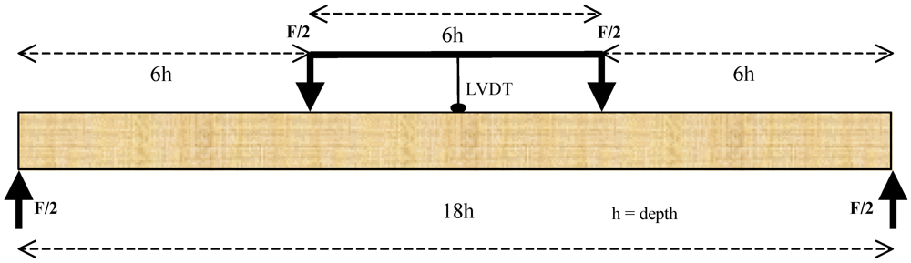
Figure 2 shows a schematic of the loading scheme.
Figure 2.
Schematic of four-point bending test set up.
Figure 2.
Schematic of four-point bending test set up.
Reinforcing timber is a means by which low grade timbers can be upgraded, or, by which timber structures can be repaired [
11]. In this test program, LVL was used because it has low variability in properties compared to low grade timbers. The number of reinforced beams tested in each series was low and focus was primarily on the effect of reinforcement geometry. Therefore, LVL was deemed an appropriate material to use to minimise variations in the composite properties that arise through the wood, as opposed to through the reinforcement and its geometry.
2.2. Model Development
Series I-IV beams were constructed according to the cross sectional dimensions shown in
Figure 3, each component for each composite beam also having a length of 900 mm. The cross sections modelled represent only one half of the actual beam cross sections due to symmetry. The modelled beam lengths were also symmetrical about their centre points and hence, only half the beam length needed to be modelled.
Node sharing contact between the beam components was specified for each beam. This assumed a theoretically perfect interface, which is infinitely thin and inseparable, even beyond the maximum bond stress capabilities of the adhesive-steel or adhesive-LVL interface. This approximation is acceptable provided there is no de-bonding between any of the adhesive interfaces throughout the duration of monitored loading (i.e., to slightly beyond the composite yield strength).
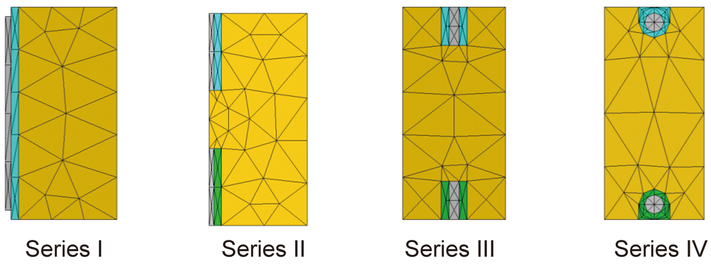
Series I-IV beam components were discretised using 1st order three-dimensional solid elements. Each element comprises eight nodes and three degrees of freedom exist at each node in the directions perpendicular and parallel to the LVL grain axis, which coincide with the orthogonal Cartesian axes x, y and z. The element edge lengths were defined according to the geometric requirements of each component within each model. The final mesh patterns for the cross sections of series I-IV composites are shown in
Figure 4.
Figure 3.
Cross sectional dimensions and layout used in finite element models for beams from series I-IV (labelled). In each series, the laminated veneer lumber (LVL) is textured brown, the adhesive is black and the steel reinforcements are shaded grey.
Figure 3.
Cross sectional dimensions and layout used in finite element models for beams from series I-IV (labelled). In each series, the laminated veneer lumber (LVL) is textured brown, the adhesive is black and the steel reinforcements are shaded grey.
Figure 4.
Mesh patterns of cross sections for composite beams in series I-IV.
Figure 4.
Mesh patterns of cross sections for composite beams in series I-IV.
Stress-strain characteristics of steel are adequately represented using bi-linear plots where the onset of yield is defined and work hardening is taken to 15% strain. The steel is assumed to be an isotropic solid with a density of 7900 kgm
−3, a shear modulus of 83 GPa, an elastic modulus of 210 GPa and a Poisson’s ratio of 0.27. Work hardening in the steel begins at the critical von-Mises stress,
σv. This stress is calculated according to the principle,
![Buildings 02 00231 i001]()
and nonlinearity begins at 300 MPa. The subscripts
1,
2, and
3 refer to the individual principal axes of the steel, which are coincident with the orthogonal Cartesian axes.
The tensile and compressive characteristics of Rotafix CB10TSS adhesive were approximated to elastic-perfectly-plastic systems. Tests were performed on clear samples of CB10TSS. Tensile tests were performed on three samples of CB10TSS, which had a thickness of 4 mm and a width of 10 mm. An extensometer was used to measure the strain as a function of loading. The values for the compressive properties of CB10TSS adhesive were provided by the manufacturer, Rotafix Ltd. The elastic moduli of CB10TSS adhesive are the same in tension and compression, however, the compressive strength of this adhesive is superior to its strength in tension.
Figure 5 shows the elastic-perfectly-plastic tensile and compressive characteristics input into the model.
Figure 5.
Elastic rigid-plastic stress-strain relationships for the adhesive in tension and compression.
Figure 5.
Elastic rigid-plastic stress-strain relationships for the adhesive in tension and compression.
The LVL was modelled as an orthotropic elastic–anisotropic plastic material with a density of 520 kgm
−3. The elastic constants are provided in
Table 1 and the Cartesian x-axis is considered parallel to the grain of the LVL. Although orthotropy is assumed, the elastic constants for the two axes normal to the direction of the grain were normalised such that; Ex ≠ Ey = Ez and υxy = υxz ≠ υyz. The values are in accordance with tests conducted at the University of Bath. The E value used here is slightly higher than the value of 12.4 GPa. This was necessary to circumvent convergence problems associated with the consistency criteria for elastic constants in the orthotropic model simulation.
Table 1.
Elastic properties of Kerto S laminated veneer lumber.
Table 1.
Elastic properties of Kerto S laminated veneer lumber.
| Property | Direction or plane |
|---|
| x | y | z | xy | yz | xz |
|---|
| E/GPa | 12.75 | 0.255 | 0.255 | - | - | - |
| G/GPa | - | - | - | 0.62 | 0.62 | 0.62 |
| ν | - | - | - | 0.03 | 0.29 | 0.03 |
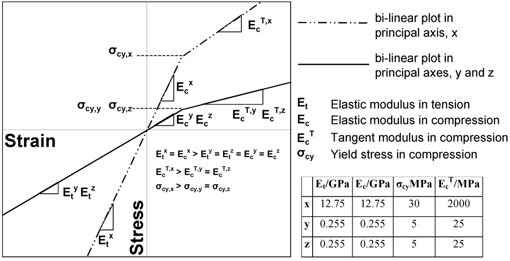
Normal yield stresses in compression, σcy, were defined in the orthotropic principal axes of the LVL, which were taken to coincide with the local orthogonal Cartesian axes, the x axis of which is normalised with the grain axis of the LVL. Yielding in tension was not specified as it was assumed that the behaviour of the LVL in tension was linear elastic throughout the duration of loading. Peak shear stresses, τp, were also identified and defined in the xy, yz and xz planes. Following yielding in compression or shear, tangent moduli and tangent shear moduli describe the plastic stress-strain relationships in each direction and plane.
It is incorrect to specify solely the non-linear compressive characteristics of LVL for beams subjected to flexure. Although such an approximation may be valid for compression dominated failure, there will certainly be the development of high tensile stresses on the underside of a bending beam below the neutral axis. Plastic incompressibility restricts the use of both tensile and compressive characteristics in the same model. The problem is overcome by linearly interpolating between the data predictions of two models, one possessing the tensile characteristics of LVL and the other with the compressive characteristics. Given that there is symmetry about the axis of neutrality prior to loading, it is plausible to assume that exactly half the beam experiences tension, whilst the other half is subjected to compression. This approximation essentially violates true beam behaviour whereby the neutral axis moves closer to the tensile edge of the beam at the onset of compressive yielding. It is however an easily applicable approximation that minimises the errors associated with leaving out the characteristics of tensile failure altogether.
The normal compressive and shear yield stresses as well as the gradients describing the 1st order (linearly) proportional plastic stress against plastic strain were determined through experimental compression and shear block testing of LVL specimens with dimensions of (50 mm)
3. These tests were conducted at a displacement rate of 2 mmmin
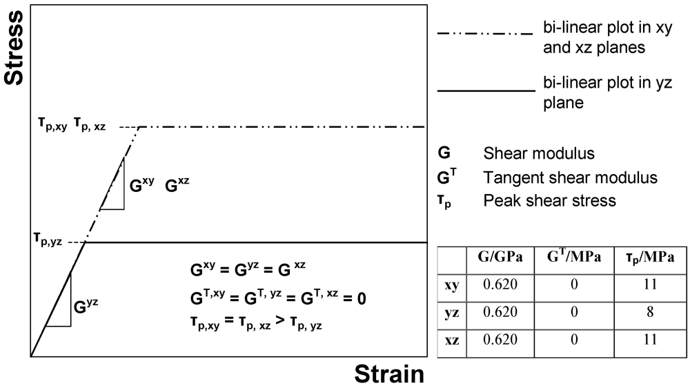
−1. The tangent moduli for the compression block tests were measured at a 0.2% proof stress. A strain of 0.2% was chosen to ensure that the slope of the tangent corresponded with the slope of the linear plastic stress-strain gradient. The bi-linear stress-strain plots for the shear planes xy, yz and xz followed the appropriate shear modulus in each plane until reaching the peak shear stress of the material, after which the plastic slope supposed a zero tangent modulus.
Figure 6 illustrates the tensile-compressive characteristics defined for the LVL, while the shear characteristics input into the model are shown in
Figure 7. Though wood failing in shear is typically brittle, perfect plasticity had to be specified to avoid convergence problems associated with sudden drops in the material parameters.
Figure 6.
Stress-strain approximations and related values for LVL in each principal axis.
Figure 6.
Stress-strain approximations and related values for LVL in each principal axis.
Figure 7.
Bi-linear stress-strain approximations and related values for LVL in xy, yz and xz shear planes.
Figure 7.
Bi-linear stress-strain approximations and related values for LVL in xy, yz and xz shear planes.
The model was symmetrised about ½l and ½b, where l is the span and b is the width of an entire composite beam such as was tested in series I-IV. Displacement controlled loading was applied via nodes attached to a line across the upper edge of the LVL segments for all beams (series I-IV). The line was located at a distance of 300 mm from the centre point of the beam. Force would be transferred therefore, through the LVL to the reinforcement via the adhesive. Nodal translations at the lower edge of the beam end were restricted in every degree of freedom along the Cartesian axes at a position on the lower edge of the beam at a distance of 900 mm along the span from the centre point of the beam. Rotational freedom was left unrestricted.


 and nonlinearity begins at 300 MPa. The subscripts 1, 2, and 3 refer to the individual principal axes of the steel, which are coincident with the orthogonal Cartesian axes.
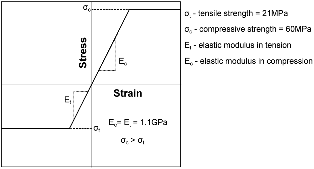
