Integrating Real-Time Room Acoustics Simulation into a CAD Modeling Software to Enhance the Architectural Design Process

Abstract

For architects, real-time 3D visual rendering of CAD-models is a valuable tool. The architect usually perceives the visual appearance of the building interior in a natural and realistic way during the design process. Unfortunately this only emphasizes the role of the visual appearance of a building, while the acoustics often remain disregarded. Controlling the room acoustics is not integrated into most architects’ workflows—due to a lack of tools. The present contribution describes a newly developed plug-in for adding an adequate 3D-acoustics feedback to the architect. To present intuitively the acoustical effect of the current design project, the plug-in uses real-time audio rendering and 3D-reproduction. The room acoustics of the design can be varied by modifying structural shapes as well as by changing the material selection. In addition to the audio feedback, also a visualization of important room acoustics qualities is provided by displaying color-coded maps inside the CAD software.

1. Introduction

Nowadays computer simulations often support the design and the engineering of rooms buildings and rooms. In acoustics, this option became feasible in the 1990s [1,2]. Before that time the acoustic design had to be based on fundamental equations which deliver a trend and information about the sound field average. Usually this involved a calculation of the reverberation time or sound transmission coefficients in order to proof the design concept and its match with the desired building performance. The acoustic component is obviously relevant for speech communication, for music perception and for the purpose of noise control. The human perception, however, is sensitive to specific features of the sound source (e.g., directional characteristics), the source signal and the sound propagation in the room or building. These features are often not sufficiently described by averages of acoustic data such as reverberation times and sound pressure levels and require more detailed investigations.

Reverberation is considered to be an extremly important phenomenon in room acoustics [3]. It generally varies for different sound frequencies. A typical value for an auditorium (e.g., a lecture hall with a volume of 800 m${}^3$) is a reverberation time of one second, with a slight increase towards bass frequencies and a decrease towards treble. It can be predicted rather precisely by using the room volume and the average absorption [4]. Other criteria, however, which describe more specifically the spatial impression, the clarity of speech, and the sensation of distance to the source cannot be predicted accurately with a similarly basic approach [5] and should rather be derived from the room impulse response.

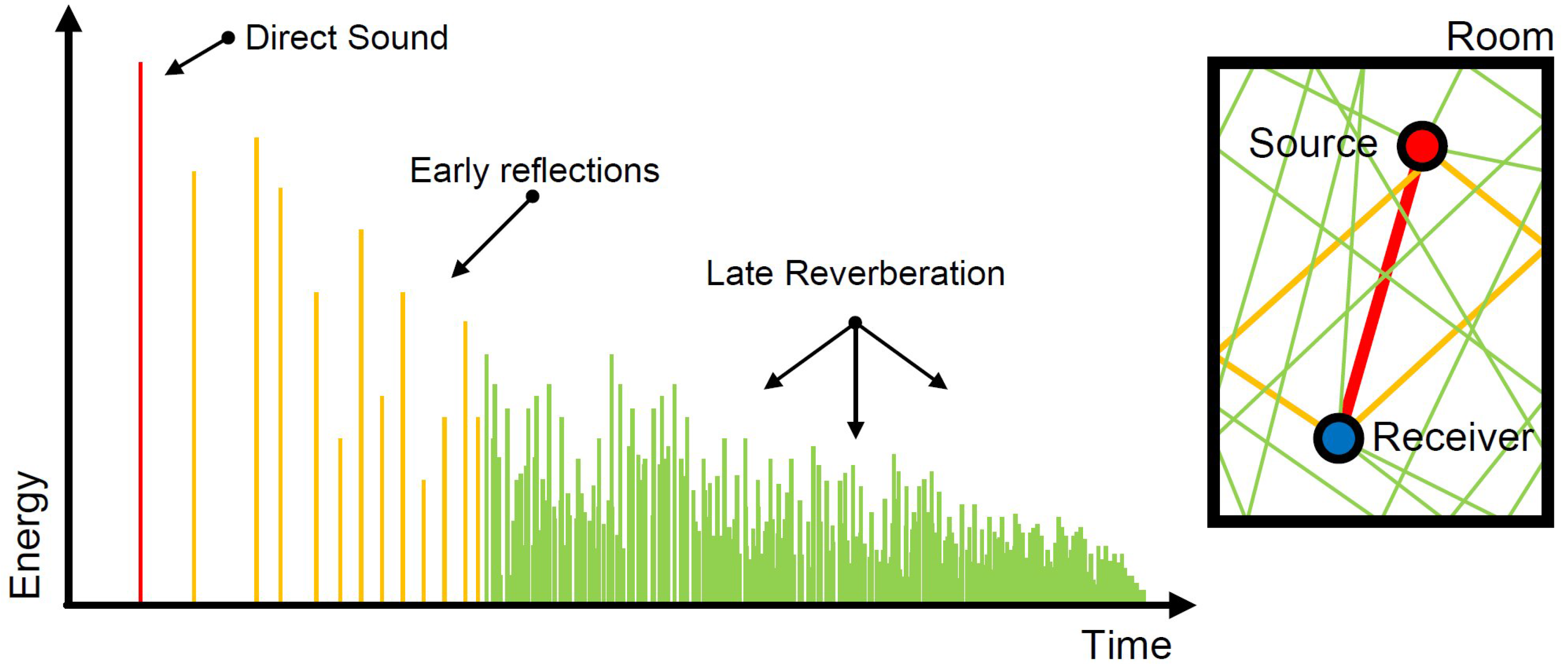
In a geometrical model, the sound travels on straight lines and loses energy due to absorption whenever a wall reflection occurs. The part on the right hand side of Figure 1 illustrates the reflection paths of the impulsive sound ray in the room, the left hand side shows the corresponding function of energy vs. time, usually called energy impulse response of the room.

Figure 1. Simplified example of an energy impulse response of a room, including direct sound, early reflections and late reverberation.

Figure 1. Simplified example of an energy impulse response of a room, including direct sound, early reflections and late reverberation.

Relevant information about the acoustic quality of a room can be derived from the impulse response. Some perceptual criteria such as reverberance, clarity of spaciousness can be obtained from post-processing of the impulse response, so that more numbers are available to analyze the acoustic quality in detail. It is convenient to visualize varying values of these room acoustic parameters at different positions in the room by using color-coded maps, as shown in Figure 2.

Room Acoustics can be discussed by evaluating the color-coded maps, followed by an adaption of the architectural design towards an improved situation. This usage of visual information, based on computer simulations, help to enhance the acoustics of the room. Imagine you have to explain a design sketch to a person who does not see it. The verbal characterization will be based on descriptors like size, color, brightness, maybe on the elements contained in the design or on resolution of details. A design exercise reproduced purely based on this description will be never exactly like the original. It will contain a lot of subjective interpretations, even if the descriptors are objective parameters. How much easier and unambiguous would it be if we just looked at the design instead of discussing its visual parameters! To compare audible situations, we shall extend the computer simulation towards an option of presenting the results directly through the sound card. This concept is called auralization [6].

Figure 2. Color-coded map overlayed into the model view of SketchUp to monitor the room acoustic parameter Clarity across a grid of positions inside a concert hall.

Figure 2. Color-coded map overlayed into the model view of SketchUp to monitor the room acoustic parameter Clarity across a grid of positions inside a concert hall.

Professionals in acoustics analyze sounds with excellent precision and they recommend excellent solutions to acoustical problems. But there are fields of acoustics where predictions can hardly be evaluated based on pure numbers, there are fields in acoustic engineering where non-experienced clients must be persuaded to invest for a better acoustic environment, there are fields of acoustic research where the process of a particular auditory perception is not finally understood. Auralization can contribute to solve some of these problems.

This paper describes a newly developed plug-in for adding an adequate 3D-acoustics feedback to the architect, based on validated room acoustic simulation models [7,8,9,10,11]. The plug-in provides real-time color mapping of room acoustic criteria, real-time auralization (audio rendering), and 3D-reproduction to present intuitively the acoustical effect of the current design project.

2. Room Acoustics Simulation

2.1. Simulation Techniques

For about the last 10 years a significant progress was made regarding the complexity and accuracy of auralization techniques. All computer models aim at calculation of an impulse response between the source and the receiver. Apart from wave acoustic models which deliver a precise solution of the room sound field with a given room shape and the acoustic impedance boundary conditions, there are models available which predict the room impulse response with approximations (e.g., assuming the dimensions of the room are large compared with the wavelength of the sound [4]). In spite of the apparent shortcomings due to the approximations these simplified models are superior due to significantly faster computation time. Furthermore they yield results which are in no way less accurate than the results from the apparently exact wave acoustic theory. This is due to the uncertainties of the acoustic input data describing the boundaries prohibit results of high accuracy [12]. The room sound field is quasi-stochastic so that even small deviations from the nominal values lead to large variations in the results [13]. Therefore most of the work on room acoustic simulation was based on geometrical methods [14,15,16,17,18,19].

2.2. Geometrical Acoustics

In geometrical acoustics, like in geometrical optics, diffraction and interference effects are neglected. The description of the sound field is reduced to the parameters energy, transition time and direction of rays. This approach is correct as long as the dimensions of the room are large compared with wavelengths and if broadband signals are considered. These approximations are valid with sufficient accuracy in rooms intended for speech and music [4,6]. The task in geometrical acoustics is to find the paths of sound connecting the source and the receiver. The total sound field, consisting of the direct sound and all reflections, must be determined. For this problem two methods are available which will be presented in the following subsections.

2.2.1. Image Sources

One of the basic algorithms in geometrical room acoustics is the image source model. The most important restriction is that modeling of sound scattering (also called diffuse reflection) is not possible. On the other hand, the great advantage is that impulse responses are not limited in accuracy as concerns the reflection delay times since it can be calculated with extremely high time resolution. Provided each wall reflection is purely specular, the image source principle can be formulated [20,21]. At first, image sources must be constructed for the room under test. The original sound source S is mirrored at each wall to construct image sources of first order. With the first-order image sources the procedure is repeated (see one example room in Figure 3). Hence sources are created which represent rays with several wall collisions, taking into account all possible permutations of the collision order due to the wall numbers. This procedure is repeated until a chosen maximum order of image sources is reached. After that, a so-called visibility test (audibility test) is carried out.

This test is receiver-dependent and checks the validity of all image sources. Each source is the last link in a chain of successive image sources and, with its indices, one can read which walls were hit by the associated ray path.

The total sound field can be composed by adding the contributions of all audible sources according to the $1/r$ law which sets as well the amplitude of each contribution as its time delay (see Figure 3). The directivity of the original source, the wall absorption and properties of the receiver can be modeled easily and with amplitude and—if necessary—phase information.

Figure 3. Room situation with two examples of audible image sources (first and second order) and their contribution to the energy impulse response.

Figure 3. Room situation with two examples of audible image sources (first and second order) and their contribution to the energy impulse response.

2.2.2. Ray Tracing

Conventional ray tracing is based on the idea of discrete sound rays or sound particles propagating on straight lines from wall to wall [14,15]. The detected energy corresponds to the number of rays hitting a receiver volume (typically a sphere) which is hence just a question of counting events. The distance law of free field energy propagation is implicitly included since the ray density and the rays hitting a receiver decreases with $1/r^2$.

Sound sources can be modeled by emitting rays with a certain power (number of rays) and directivity (distribution of rays or direction-dependent ray energies). As it has to be called very often, the procedure for handling wall reflections is a very important part of the algorithm. A point-in-polygon test is the crucial subroutine which must be implemented in the software in the most efficient way. A detection is happening if the distance of the ray to the receiver position is smaller than the detector’s radius. The rays are reflected according to Snell’s law with incident angle and the reflected angle being equal. Rays can also be scattered according to Lambert’s law [22,23]. Absorption in case of a reflection is modelled by multiplication with the factor $(1-\alpha )$ with α denoting the absorption coefficient. In case of detection, the energy and the transition time is recorded in time intervals (typically some milliseconds). The results are energy histograms, e.g., low resolution energy impulse responses as illustrated in Figure 4.

Such energy decay curves can further be processed for various single number quantities. According to ISO 3382 [24], important parameters are Strength G, Definition D, Clarity C, Early Decay Time EDT, Lateral Energy Fraction LF, etc. If impulse responses have been calculated for complete audience areas, the single number quantities can be visualized in color maps (example in Figure 2).

2.2.3. Hybrid Models

Deterministic models such as the image source model suffer from errors introduced by the model itself (lack of diffuse reflections) and by limitations of geometrical acoustics in general. Due to contradictory disadvantages ray tracing and image sources are combined in order to achieve high precision results without spending too much computation time [25,26,27]. Either ray tracing algorithms are used for simulation of the late part of the impulse response (adding a reverberation tail) to overcome the exponentially increasing calculation time of the image source model, or ray tracing is used to detect audible image sources in a forward audibility test. The latter procedure is named cone tracing or beam tracing [28,29]. Almost all other algorithms used in commercial software are similar versions of these algorithms, depending on the type of results, particularly on the accuracy, spatial and temporal resolution. One important example for specific demands is the so-called Auralization [2,6], where the simulated impulse responses are intended to be used for filtering reverberation-free (dry) speech or music.

Figure 4. The ray tracing algorithm returns histograms which define the temporal envelope of the energy decay in the room. It is run for different frequency bands (shown in different colors) separately.

Figure 4. The ray tracing algorithm returns histograms which define the temporal envelope of the energy decay in the room. It is run for different frequency bands (shown in different colors) separately.

2.3. Room Model

2.3.1. Room Geometry for Geometrical Acoustics Simulations

In computer aided design (CAD), models of buildings or objects are typically defined by a set of points. Every point belongs to at least one group, forming a polygon, which consists of three or more vertices in total. Non-structural information can be applied to the polygon by adding a texture. While textures are especially important for the visual appearance, additional information, such as acoustical characteristics (absorption and scattering coefficients) can also be assigned to each polygon. Such acoustic material properties are discussed in Section 2.3.2

In contrast to computer graphics, a highly detailed model is not desired for acoustics calculations, as it does not lead to a more accurate result of the room acoustic simulation. A proper room model for a geometrical acoustics simulation should not contain structures smaller than the observed wavelength. The human ear is capable of perceiving sound within a frequency range from 20 Hz to 20 kHz, corresponding to acoustical wavelengths from 17 m to 1.7 cm. A usual loss of sensitivity of our hearing and a much higher rate of air absorption in the higher frequency range makes a spatial resolution of 50–70 cm a sufficient choice for the input model of the room acoustic simulation [30]. The reduction of the details of the model benefits the computational workload of the acoustical simulation while ensuring correctly modeled reflections. A model with less polygons requires less testing for intersections of the sound propagation paths and thus reduces the total computation time significantly. This is another reason why for acoustic simulations usually a separate model with a lower level of detail is created, although in some cases a highly detailed model for the visual appearance already exists. Figure 5 shows an example of a room, including the normal and the acoustical room model.

Figure 5. Two models of a church—the simple model on the left side functions as the input data for the acoustical simulation, while the high detailed model (right) is used for visual representation.

Figure 5. Two models of a church—the simple model on the left side functions as the input data for the acoustical simulation, while the high detailed model (right) is used for visual representation.

To adapt to the behavior of sound waves in different frequency ranges, also a level-of-detail implementation can be considered for room acoustics simulation [30]. While the model for the higher frequencies contains structures of sizes down to 50 cm, the simulation of the lowest frequency bands is based on a model with structures of 5–10 m. This may not only lead to more accurate results, but also to significantly reduced calculation time of the ray tracing algorithm. Calculation methods for the automatic level-of-detail reduction of high detailed models have also been developed [31,32].

2.3.2. Material Properties

Whenever a sound reflection at a wall occurs, the properties of the material of the reflecting object have to be considered [23]. In case of a reflection not only the direction of the waves is changed, the wave also loses energy. This change in amplitude (and phase γ) is usually described by the complex reflection factor R. It consists of a factor $\left|R\right|$ expressing the fraction of the reflected sound wave and of a phase shift γ [33]. However, for the calculation models of geometrical acoustics it is sufficient to describe a wall reflection by the absorption coefficient $\alpha =1-{\left|R\right|}^2$. In the simulation algorithm, the absorption coefficient of the corresponding wall reduces the amount of energy (of the sound ray or the image source) whenever a reflection on that wall has happened. Because the absorption might differ significantly within the audible frequency range, the absorption coefficient is usually given as a list for multiple frequency values (see Figure 6).

Depending on the structure of the wall, not every wall reflection is a specular reflection. If the wall surface structures are not very small or very big compared to the wavelength the sound wave is scattered. This property of the material is usually expressed by the scattering coefficient, which is, because of the relation to the wavelength, also dependent on the frequency. The scattering coefficient describes which amount of energy is reflected in other directions than the specular path. It is considered in the ray tracing algorithm and often implemented as a stochastic process.

Figure 6. Acoustical properties of an example material (wooden structure). Absorption coefficients (purple) and scattering coefficients (blue) are shown from 20 Hz upto 20 kHz.

Figure 6. Acoustical properties of an example material (wooden structure). Absorption coefficients (purple) and scattering coefficients (blue) are shown from 20 Hz upto 20 kHz.

Both coefficients have a value between 0 and 1, that can be determined for different materials by various measurement techniques [23]. Because the absorption reduces the energy of the sound field inside the enclosure, while the scattering only changes the distribution of the sound field, absorption is often regarded to be much more important than the scattering coefficients of the wall materials. Nevertheless there is a need to consider scattering coefficients in room acoustic prediction algorithms [3,34] and it has be shown that different scattering coefficients can be distinguished by a listener [35].

Next to the material properties, also parameters of the air inside a room are considered in the room acoustics simulation. Air pressure, temperature and humidity determine the speed of sound as well as the air absorption and thus influence the sound propagation inside the room.

2.3.3. Spatial Data Structures

During the calculation of sound propagation paths within the image source or ray tracing algorithm, testing whether a path intersects a polygon of the scene is the most frequent operation. In the most inefficient way of implementation, all polygons have to be checked for an intersection. This raises the computational effort drastically, especially for room models with a high polygon count. To avoid situations of such demanding computational effort, spatial data structures can be applied to the room model. Binary Space Partitioning (BSP) [36] recursively divides the room into two subspaces by partitioning planes and arranges the subspaces in a tree structure (BSP tree), which reduces the number of intersection tests. Spatial Hashing (SH) [37] is another concept, which divides the space in primitive volumes of equal size, storing information in a hashmap. In comparison, intersection tests using the BSP concept are faster, however the SH concept is more suitable if the geometry of the room is often modified and the simulation result shall be provided as instant as possible. This is because the update of the BSP tree is a costly operation, whereas the update of the hashmap in case of a geometry modification is faster [38]. Thus, during static situations of the geometry, the BSP concept should be used, while in dynamic scenarios, the SH method is the more efficient choice [39]. To benefit from the advantages of both spatial data structures, the room acoustic simulation software presented in this article is using both concepts in a hybrid approach. Figure 7 shows the process of the creation of spatial data structures, starting with the SketchUp model, which is translated into a polygon representation, functioning as the input data for the generation of two different spatial data structures, which are then used for the intersection tests of the simulation algorithms.

Figure 7. Generation of spatial data structures to speed up intersection tests and reduce the computational workload of the room acoustic simulation.

Figure 7. Generation of spatial data structures to speed up intersection tests and reduce the computational workload of the room acoustic simulation.

3. Implementation

The room acoustics simulation module, called RAVEN (Room Acoustics for Virtual Environments), is implemented as an C++ library that can be linked into existing projects [39]. It makes use of many modern optimization techniques, such as multi-core parallelization and utilization of extended instruction sets. This makes it a high performance library that can take advantage of the full computation power of modern CPUs.

Because of the numerous occuring reflections in the reverberation tail, the most time-consuming part of the operation of the simulation is the ray tracing, which can take between seconds to minutes of time, depending on the amount of required rays and the complexity of the room model. However, the calculation time can be reduced significantly by distributing the workload to two or more parallel threads, e.g., on a multi-core CPU. This can be done as the reflection paths of one ray does not depend or interfere with any other rays. The threading concept is addressed in detail in Section 3.3.

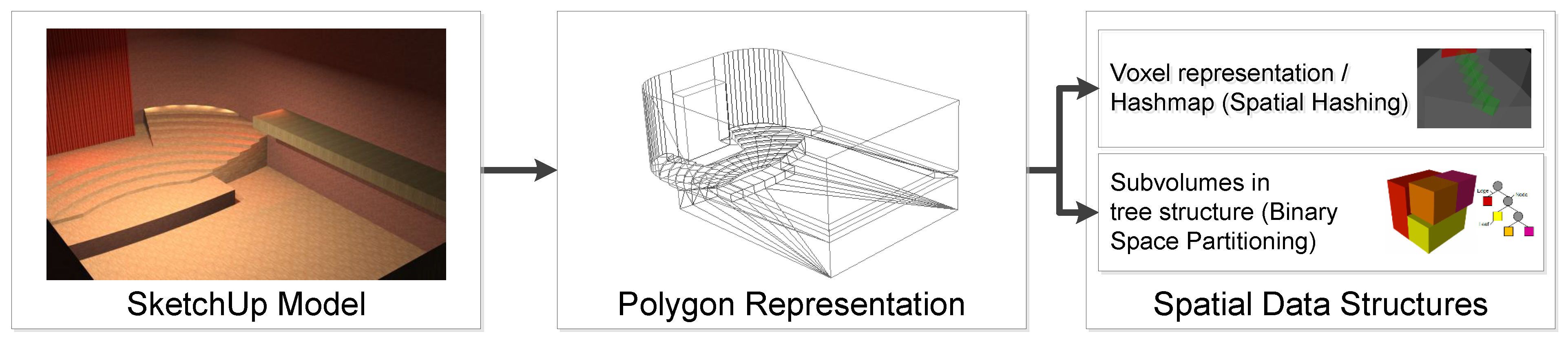
Another technique to cut down the computation time of ray tracing and also image source calculations was earlier introduced in Section 2.3.3 with the usage of advanced spatial data structures for handling the polygonal room model. To constantly transfer the room model from the 3D modeling GUI to the acoustics simulation environment, a plug-in was developed and integrated into the 3D modeler. A detailed description of this plug-in is given in the following Section 3.1.

The most important reason for extending a 3D modeling tool using a plug-in architecture is the possibility to seamlessly integrate into the user’s work flow, especially if he is an architect who can then remain using his familiar software environment. But also from the point of view of an acoustics-oriented user the professional 3D modeling programs usually offer a better experience for 3D editing compared the internal 3D editors of the room acoustics programs.

This is also the reason why most acoustics simulators nowadays offer an import option for common 3D file formats, e.g., import from AutoCad (*.dxf), Autodesk 3ds Max (*.3ds) or SketchUp (*.skp). However, the necessary sequence of exporting and importing the model is a tedious and time consuming process. Additionally, due to the strict separation of the 3D construction and the acoustics simulation there is no interactivity or intuition in between these processes.

Furthermore typical room simulators can only be handled by acoustic experts. The output is not readable without having a strong background in acoustics and results are often difficult to interpret. Some modern programs offer an auralization option, which enables an intuitive way to observe the results by listening to the room. This provides the experience of acoustic feedback in a similar quality as the visual 3D representation. In currently available programs though, the auralization feature is only available after another time consuming calculation and processing step. The resulting interrupt between design action and acoustic reaction avoids to observe, understand and control the acoustics implications during the design process in a similarly intuitive and effective way as it is available for the visual sensation.

Therefore the simulation and auralization options were integrated using the plug-in extension so that results can be shown inside the 3D working environment and a direct visual and acoustic feedback of the sound of the room can be provided to the user. Details of the real-time processing implementation are described in Section 3.3, Section 3.4 and Section 3.5.

3.1. Selection and Extension of the CAD Software

The choice of a suitable 3D modeling software was driven by the expected composition of future users. A main part of users would be architects (professionals, students, teachers), but also acoustic consultants and students. Because of the real-time audio options also sound engineers are a group of interested users. Due to the mixed experience in 3D modeling of these groups the CAD software is required to be user friendly and easy accessible by inexperienced users, yet the modeling tool should also be suitable for professionals. Another main criterion was the ability to extend the software using an API (Application Programming Interface) or a plug-in architecture. Luckily many modern programs offer such interfaces and can be extended with self-developed modules. The first choice for a prototype implementation was the Trimble SketchUp software (http://www.sketchup.com) (formerly belonging to Google), which is known to be a very popular and easy to use tool that can load extensions. A plug-in was developed in the Ruby programming language [40].

The main function of the plug-in is the transport of 3D geometry data, but also additional data has to be transfered to the room acoustic simulation. This includes the selection of materials to room surfaces, the positions of sound sources and receivers (points or surfaces), the selection of directivities for sources and receivers, the configuration of the simulation parameters, the input audio files or sound card channels for auralization, etc.

Controlling this input data is always related to the actual scene objects. For example, exchanging the receiver characteristics of a placed dummy head is realized by right-clicking the actual head model in the scene and selection the option from the context menu. This directional information of the receiver is included and described by a HRTF database (head-related transfer function [41,42]). Acoustic material data is hidden in the internal SketchUp Paint Bucket dialog which is the standard tool for applying materials. The absorption and scattering data can then be shown through another dialog, as shown in Figure 6. Most of the functions could be placed in standard dialogs, a toolbar or context-menus and only a few functions have to be accessed through a drop-down menu.

Not only SketchUp, but many of the most popular 3D modelers have the ability load extensions, mainly using plug-ins written in C++ or Python. Table 1 shows an overview of a selection of modelers with information on their ability to be extended (This information is supplied without liability).

Table 1. Popular 3D modeling software and their possible plug-in extensibility.

3D Modeling Software	Windows	Mac OS	Linux	Plug-in Architecture
Autodesk AutoCAD	√			Visual Basic, .NETScript
Autodesk 3ds Max	√			C++, MAXScript
Autodesk Maya	√	√	√	C++, Maya Embedded Lang. (MEL), Python
Blender	√	√	√	Python
Daz3D Hexagon	√	√
Daz3D Carrara	√	√		unknown
flexiCAD Rhinoceros	√			C++, Python, RhinoScript (Visual Basic, C#)
Inivis AC3D	√	√	√	Tool command language (TCL)
MAXON Cinema 4D	√	√		C++, Python, COFFEE
NewTek Lightwave 3D	√	√		C++, Python, LScript
Nevercenter Silo	√	√		C++
Trimble SketchUp	√	√		Ruby

Table 1. Popular 3D modeling software and their possible plug-in extensibility.

3D Modeling Software	Windows	Mac OS	Linux	Plug-in Architecture
Autodesk AutoCAD	√			Visual Basic, .NETScript
Autodesk 3ds Max	√			C++, MAXScript
Autodesk Maya	√	√	√	C++, Maya Embedded Lang. (MEL), Python
Blender	√	√	√	Python
Daz3D Hexagon	√	√
Daz3D Carrara	√	√		unknown
flexiCAD Rhinoceros	√			C++, Python, RhinoScript (Visual Basic, C#)
Inivis AC3D	√	√	√	Tool command language (TCL)
MAXON Cinema 4D	√	√		C++, Python, COFFEE
NewTek Lightwave 3D	√	√		C++, Python, LScript
Nevercenter Silo	√	√		C++
Trimble SketchUp	√	√		Ruby

3.2. Interfaces

The plug-in itself does not implement any room acoustics simulation and auralization, but it is used to channel data between the 3D editor application and the C++ acoustics simulation library RAVEN. Therefore the main task is to collect user input and provide an interface to establish a transport layer. The connection is established using the TCP/IP protocol and the messages are sent in the JavaScript Object Notation (JSON) format. This enables to interface different programs on a single computer but also enables to connect programs that run on different machines. These computers can also run different operating systems. 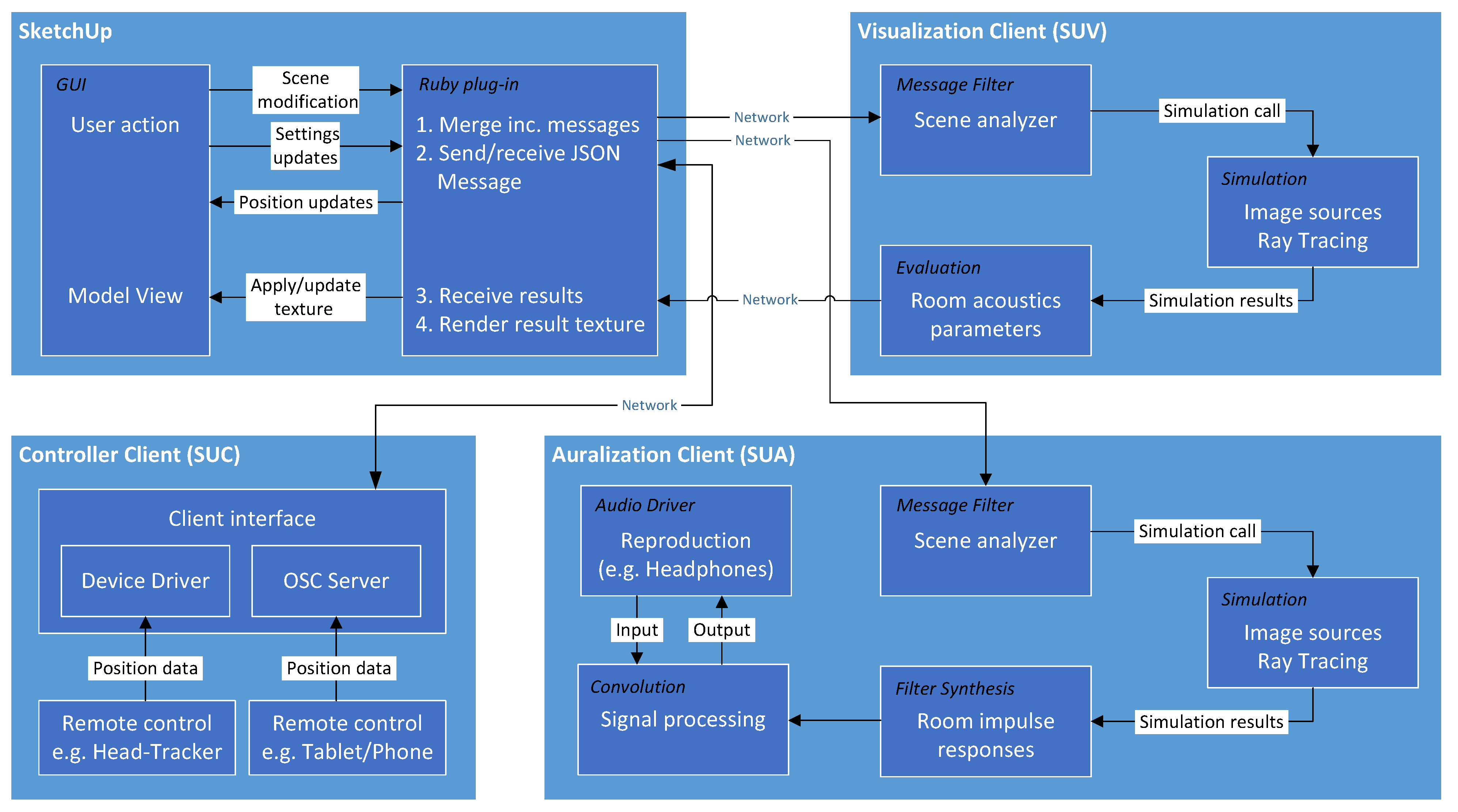SketchUp is available for Windows and Mac (also see Table 1) and the RAVEN library code is widely platform-independent. The plug-in extension opens a TCP/IP server, which allows multiple clients to connect. The current implementation allows three types of clients:

SketchUp 

Visualization Client (SUV). The visualization client runs a full simulation, calculates room acoustic parameters and returns the results back to the plug-in. See Section 3.4.

SketchUp 

Auralization Client (SUA). The auralization client(s) run(s) a full simulation, calculates room acoustic impulse responses which are applied in real-time convolution with source audio signals for sound card playback. See Section 3.5.

SketchUp 

SketchUp Controller Client (SUC). Scene information (geometry, positions, settings) is shared with the controller instance(s) in a bidirectional connection. External controllers can read and modify all SketchUp internal data. Useful to implement remote controls or automation through time sequencing.

The possibility to connect to multiple instances enables the simultaneous use of visualization and auralization, so that room acoustics parameters and the live audio feed from the room can be checked at the same time. Multiple clients running on different computers also allow the distribution of the workload. The concept is shown in Figure 8.

Figure 8. Modular structure of the SketchUp plug-in and connected simulation and control client instances. Events and messages are transmitted through TCP/IP network.

Figure 8. Modular structure of the SketchUp plug-in and connected simulation and control client instances. Events and messages are transmitted through TCP/IP network.

3.3. Simulation Concept

Details of the main simulation algorithms - the image source method and ray tracing - have been introduced in Section 2. This section focuses on the communication and sequence of interaction and simulation processes. A main concept of the implementation is the filtering of information. The numerous events during the work with SketchUp are channeled into compact and meaningful JSON messages, which are transferred to the clients (SUV/SUA/SUC) at a maximum update rate of 30 Hz. On the client side, a second filtering step is applied: A message filter called Scene Analyzer determines the impact of the modification. As not every change to the scene requires a full simulation including image source generation, audibility test, ray tracing and impulse response synthesis the Scene Analyzer selects and prioritizes the necessary simulation tasks. An overview of events and simulation actions is given in Table 2 for a connected auralization client (SUA). The visualization client (SUV) is not affected by the filtering, in the current implementation a full simulation is run on any event that has impact on the resulting room acoustics parameters.

Table 2. Examples of SketchUp events and the resulting simulation tasks after scene analysis. Brackets in the Ray Tracing column indicate that only after significant translations (>1 m) the algorithm has to be run again.

Object	Event	Generate IS	Translate IS	Audibility IS	Ray Tracing	IR Synthesis
Receiver	Rotate					√
	Translate			√	(√)	√
	Directivity					√
Source	Add	√		√	√	√
	Rotate					√
	Translate		√	√	(√)	√
	Directivity					√
Room	Material				√	√
	Geometry	√		√	√	√

Table 2. Examples of SketchUp events and the resulting simulation tasks after scene analysis. Brackets in the Ray Tracing column indicate that only after significant translations (>1 m) the algorithm has to be run again.

Object	Event	Generate IS	Translate IS	Audibility IS	Ray Tracing	IR Synthesis
Receiver	Rotate					√
	Translate			√	(√)	√
	Directivity					√
Source	Add	√		√	√	√
	Rotate					√
	Translate		√	√	(√)	√
	Directivity					√
Room	Material				√	√
	Geometry	√		√	√	√

The scene analyzer has also the task to distinguish between messages that are relevant for visualization or auralization, dependent on the type of the module (either SUV or SUA). In case of multiple SUA instances this includes a check if the affected sound source is calculated by the current instance.

Because of the high amount of receiver points, the workload of the SUV is much higher than the workload of the SUA. While the auralization runs only one receiver (the listener), the visualization is done for a grid of a couple of hundred receivers at the same time. In very complex rooms (multiple hundred faces) the SUV’s response can take up to minutes, for less detailed rooms the simulation takes less than a minute on a modern PC. For detailed calculation times, the interested reader is referred to literature [39]. In addition there are no efficient updates such as receiver translation or rotation (compare Table 2) in the visualization mode, so nearly all updates require a full simulation. The threading concept for the SUV is reduced to the implementation of openMP-parallelization for the costly image source generation and ray tracing algorithms which are run sequentially one after the other. The SUA module makes use of a parallel processing concept running diverse processes in concurrent threads which are assigned with different priorities. An example of the concurrently running threads is described in Section 3.5 and shown in Figure 13.

3.4. Visualization of Room Acoustic Parameters

Following the idea of interactive design and direct feedback, the visualization of room acoustics parameters is integrated in the modeling area of the CAD software. Any face in SketchUp can be selected as an receiver area by right clicking on the surface. This face will be removed from the regular room geometry and will be allocated with a texture that shows the results of the simulation, as shown in Figure 9. To facilitate the creation of receiver faces that are above seating areas, it is also possible to select the polygon(s) that define the floor of an audience area and select the option Create audience area from the overloaded context menu. This will automatically create receiver faces in 1.20 m (ear-)height above the the floor (also works for ascending floors).

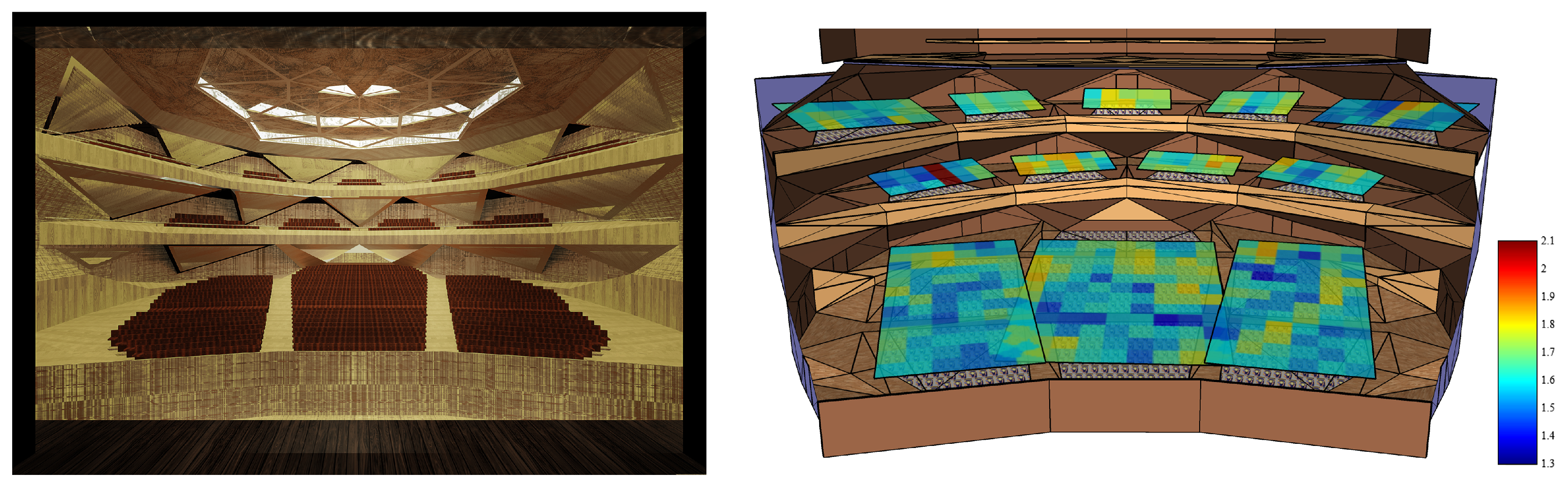
Figure 9. Design sketch of an opera house (left) and the visualization of Early Decay Time (EDT, right) directly in the SketchUp model. The color-scale was compressed on purpose to amplify small deviations of the parameter.

Figure 9. Design sketch of an opera house (left) and the visualization of Early Decay Time (EDT, right) directly in the SketchUp model. The color-scale was compressed on purpose to amplify small deviations of the parameter.

The plug-in transmits the faces’ coordinates and the acoustics module runs a single simulation for all receivers at the same time using an optimized multi-receiver ray tracing implementation. All relevant room acoustics parameters are calculated right away and transmitted back to the SketchUp plug-in. Inside the plug-in a texture is generated using the current setting of the room acoustic parameter to be shown, the selected frequency and a color-map that accounts for the selected range of values (optional auto-ranges to the minimum and maximum values). The texture(s) are assigned to the receiver faces with a light transparency so the resulting room acoustics parameters can directly be viewed inside the 3D modeling editor.

When changing the parameter selection or the color scale the results are immediately updated very due to the local calculation of textures. Only when changing the selected frequency a new simulation call is required. Once results are available for multiple frequencies the plug-in caches the results making it is possible to quickly switch between frequencies. Upon any relevant change to the room model or source/receiver configuration the cache will be cleared and a full simulation run becomes necessary again. If the available computation power is sufficient the textures are updated within a few seconds (for simple cases even less), enabling an intuitive design with short waiting periods. By saving the model (using the standard SketchUp save function) also the current simulation results are stored and are restored automatically after loading the saved model.

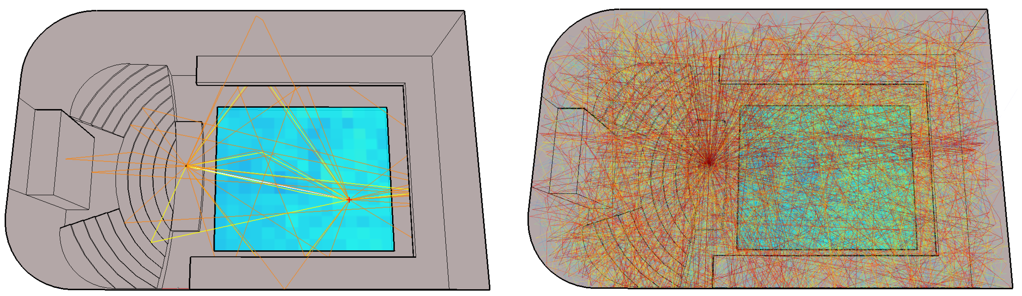
Further rendering options include the visualization of image source reflection paths and ray traces as shown in Figure 10. For the early reflections (image sources, left) the current mouse cursor position is used as receiver point and updates follow the mouse in real-time. For the ray tracing (right) it is recommended to reduce the number of particles for a clearer view as done for this plot.

Figure 10. Visualization of modeled reflections in a concert hall. Early reflections are shown using the mouse cursor as receiver point (left) and a selection of traced rays can be overlayed (right).

Figure 10. Visualization of modeled reflections in a concert hall. Early reflections are shown using the mouse cursor as receiver point (left) and a selection of traced rays can be overlayed (right).

3.5. Real-Time Auralization

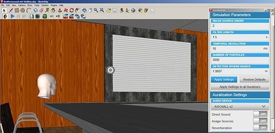
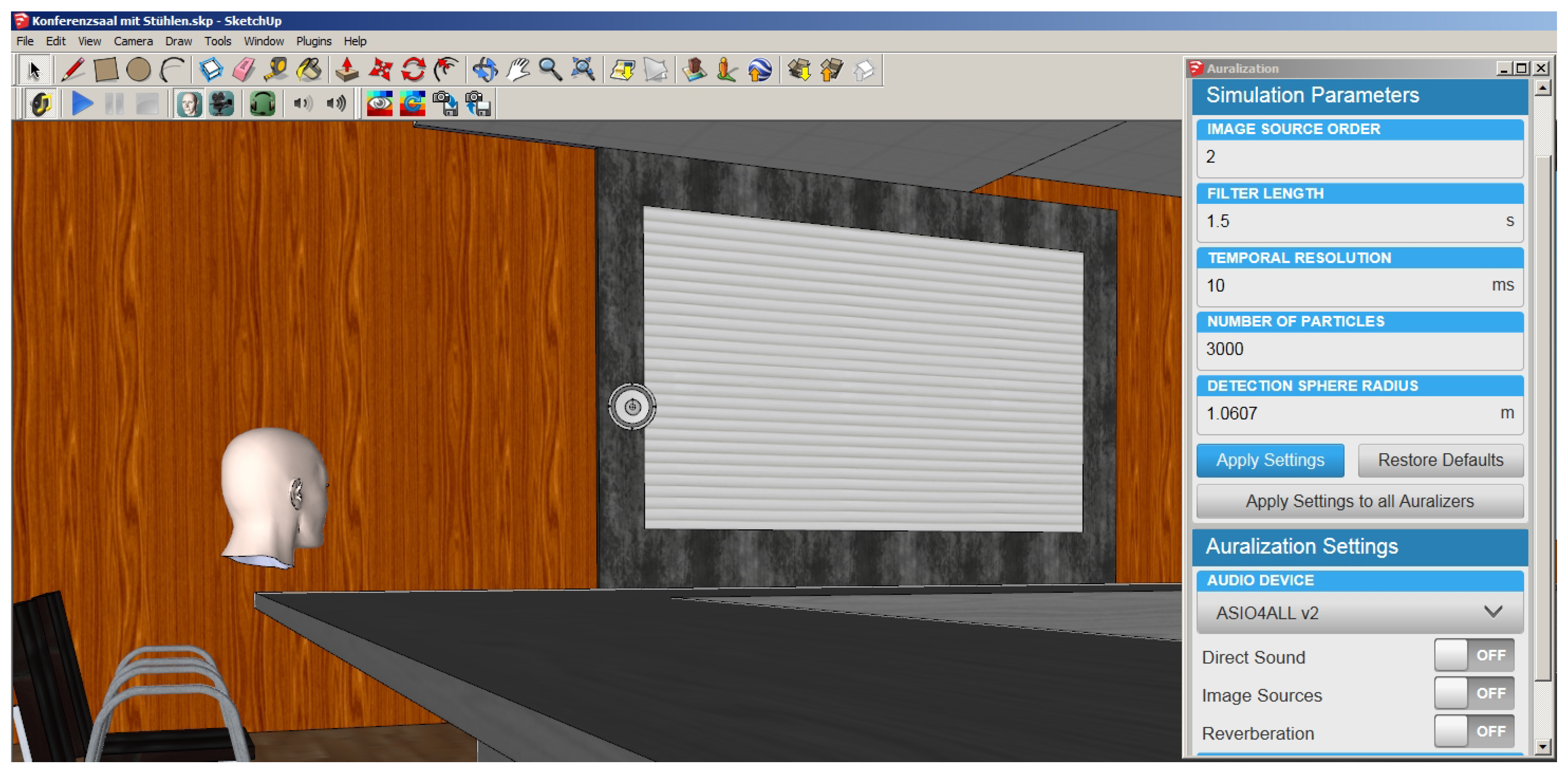
The receiver position for auralization is indicated by placing a virtual artificial head into the room, as shown in Figure 11. By right-clicking the artificial head in the 3D editor, the context menu is extended with functions to select the active head (in case of multiple receivers in the room) and the option to select different HRTF databases. It is also possible the select the position of the virtual camera of the 3D model view as the active receiver position. In this way the acoustics of the scene can be experienced in a first-person point of view, which provides a high degree of immersion and facilitates to navigate through the scene with a maximal benefit of the real-time auralization.

Due to the fact that the auralization is usually done for only one receiver position (the listener), the simulation times are significantly reduced compared to the visualization module. However, while visualization results are shown for only one sound source, the auralization will often be used with multiple sound sources. Together with the increased workload due to filter synthesis and convolution the demand on computation power is still high and the implementation must be optimized to run on common hardware with the desired real-time capabilities.

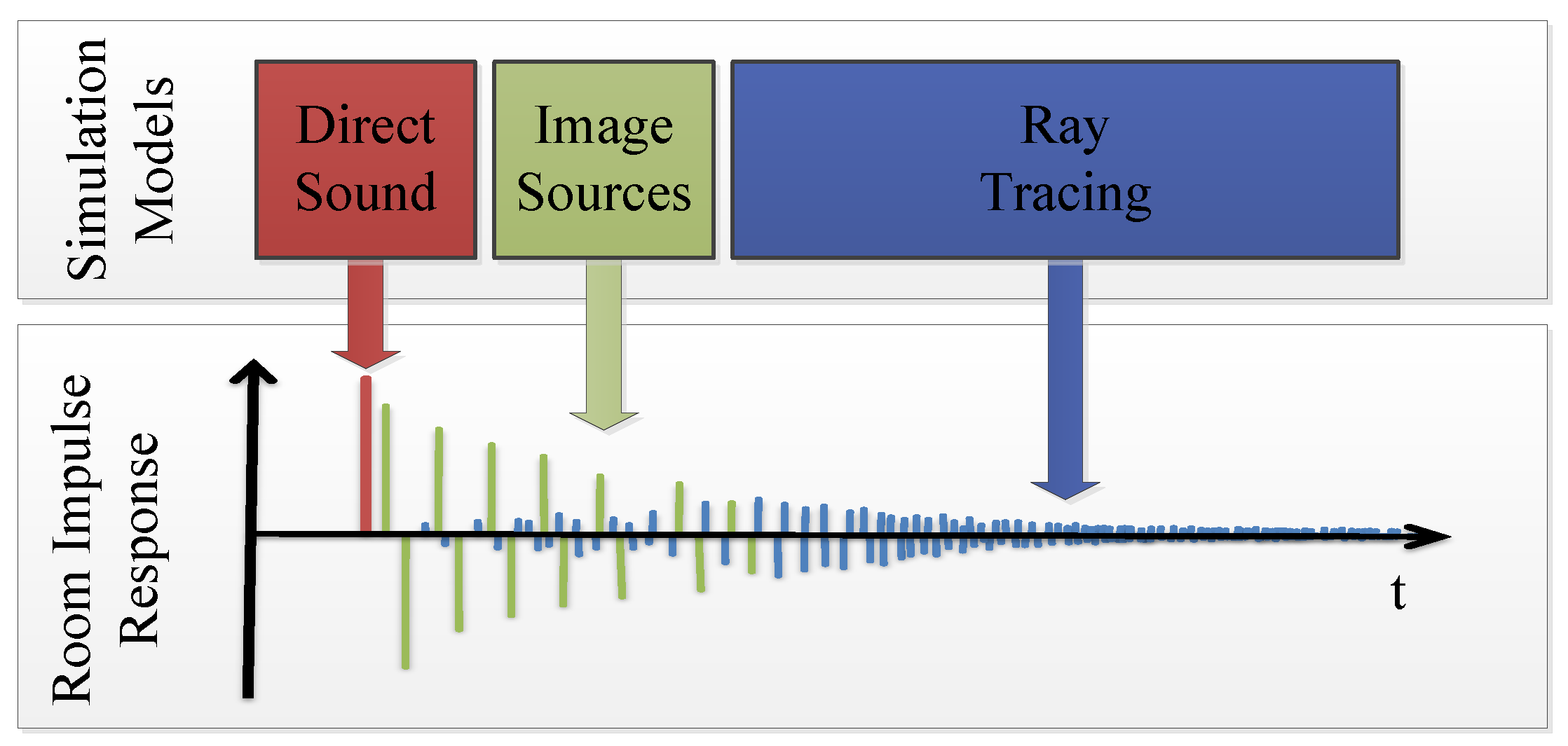
The implementation makes use of psychoacoustic effects (masking effect, precedence effect [43]) in a way that perceptually dominant events of sound sources in rooms are calculated with higher priority to increase their update rate. Currently the partial contributions of direct sound, early reflections and late reverberation are separated and individually calculated and reproduced, as shown in Figure 12. The direct sound changes quickly and significantly on source or receiver movements and is consequently updated at an increased rate with higher priority. The late decay changes only slightly while moving through a room and is also less sensitive to higher latencies, therefore the late reflections are updated at reduced rate and its calculation has lower priority. Early reflections are also important to be updated quickly, especially on listener head rotations, but are psychoacoustically masked by the direct sound and thus a little less sensitive to latency. Therefore their update rate is kept at a medium level and priority.

Figure 11. Auralization module SketchUp: Loudspeaker and artificial head define source and receiver positions. Simulation parameters are configured in the dialog on the right side.

Figure 11. Auralization module SketchUp: Loudspeaker and artificial head define source and receiver positions. Simulation parameters are configured in the dialog on the right side.

Figure 12. The impulse response is composed by superposition of three simulation methods. A line-of-sight test is used for direct sound and the image source method for early reflections. The reverberation decay is calculated using ray tracing.

Figure 12. The impulse response is composed by superposition of three simulation methods. A line-of-sight test is used for direct sound and the image source method for early reflections. The reverberation decay is calculated using ray tracing.

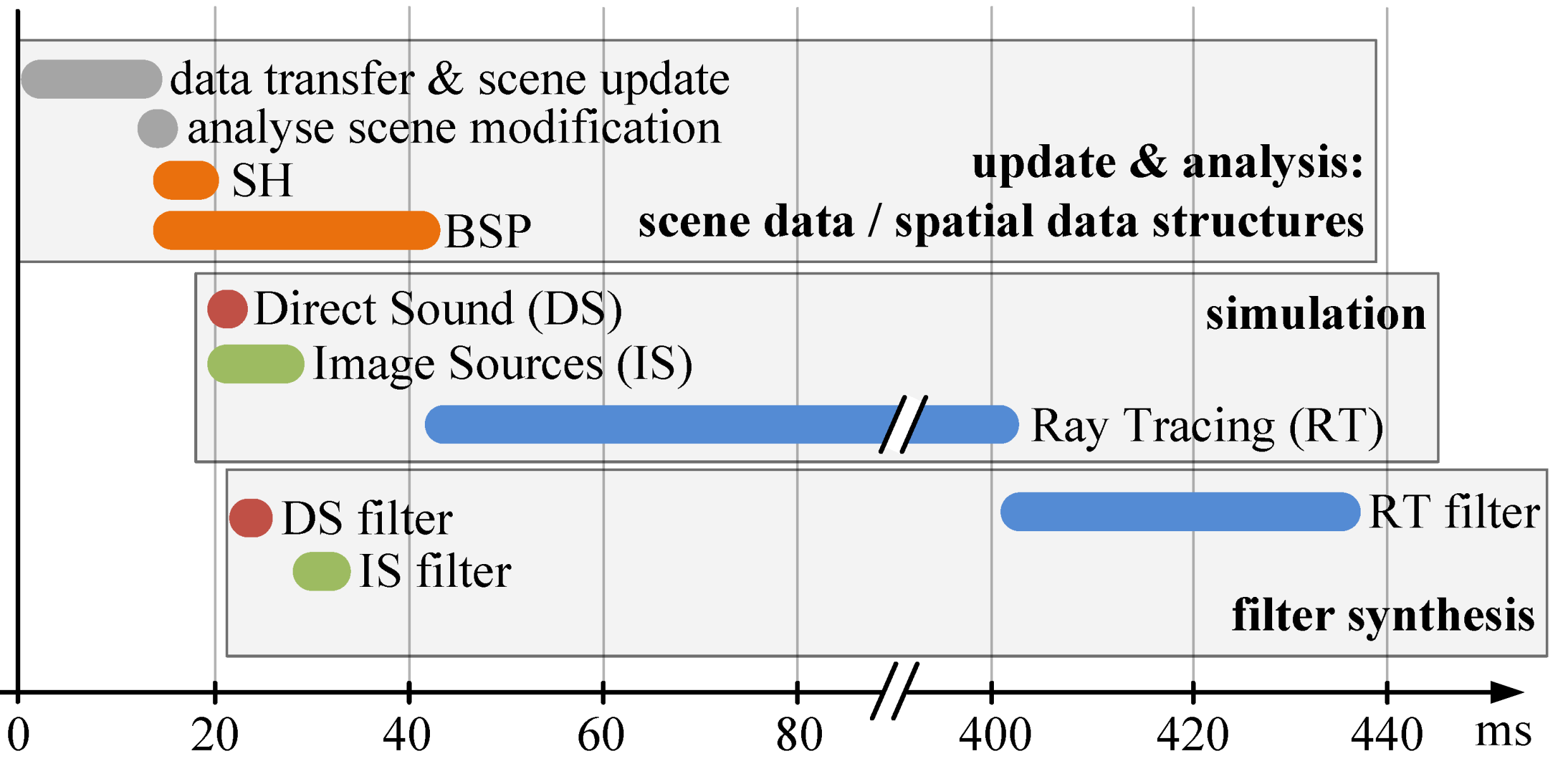
The threading concept introduced in Section 3.3 using psychoacoustically optimized priorities allows a very fast perceptual system reaction. Figure 13 shows an example of the concurrently running threads on the event of a geometry modification in a concert hall with a reverberation time of 2 s. It can be seen that although the whole simulation process takes about 440 ms the very important direct sound component is replaced in the streaming convolution after only 25 ms. The early reflections are updated after 35 ms (Image Source order 1). The psychoacoustically dominant part of the room impulse response is therefore updated with very low latency, so that a real-time experience is enabled. The calculations were done on a common desktop computer (Intel Core i7 @ 3.40 GHz, 8 GB RAM). The ray tracing simulation (about 400 ms) was executed with 1500 particles for each of the ten octave bands.

The input signal for the auralization (which is convolved with the room impulse response) can either be a sound file that is assigned to a certain source in the scene or the direct live feed from the sound card’s input jack. The latter method enables to use a microphone and talk into the virtual room while editing the scene. Also playing a music instrument while optimizing the stage or room acoustics is possible.

Figure 13. Timeline of a simulation update after a geometry modification outlining the synchronous execution of concurrent threads. The first update (direct sound) is complete after 25 ms while the whole impulse response is fully exchanged after a total of 440 ms.

Figure 13. Timeline of a simulation update after a geometry modification outlining the synchronous execution of concurrent threads. The first update (direct sound) is complete after 25 ms while the whole impulse response is fully exchanged after a total of 440 ms.

3.5.1. 3D Sound Reproduction

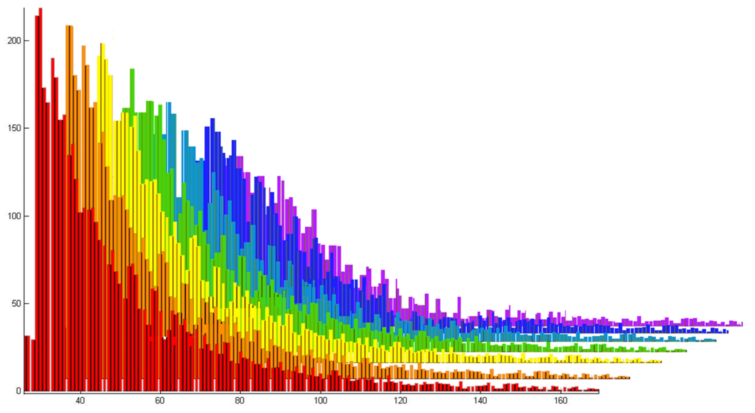
In general the acoustics simulation returns data about the incident spectral sound energy over time at a receiver position from a sound source in a room. A typical impulse response of a room with 2000 m${}^3$ volume and 1 s of reverberation contains about $100,000$ individual reflections [4]. For auralizations the direct sound and each of these reflections is spatially coded, so that the listener perceives them from the correct direction, and with correct level and spectrum which is defined by absorption through air and wall reflections. The spatial coding itself, i.e., the 3-dimensional placement of sound events, can be done in different ways, with a first decision to be made between reproduction through headphones or loudspeakers.

The headphone spatial audio coding, also called binaural reproduction [44,45], is the prefered reproduction method of for the auralization tool. It accurately emulates the ear drum signals that a human listener receives from a natural sound source from a certain direction [46]. A drawback of binaural processing is the mismatch between binaural signals taken from artificial heads compared to the ear responses of individual listeners, which degrades the localization performance [47].

For the alternative reproduction on loudspeaker systems several methods exist. These range from the simple extension of the intensity panning method (known from home stereo or 5.1 systems) to full 3D (incorporating height information) up to chains of complex signal encoders and decoders. Besides the vector-base amplitude panning [48] as a representative of the simpler methods, also a higher-order Ambisonics encoder and decoder [49] are implemented into the presented auralization module.

Advanced signal processing also allows the playback of binaural signals (initially meant for headphones) through loudspeakers. This technique is called crosstalk cancellation (CTC) [50]. Although this method is very sensitive and can introduce spectral coloration it provides a good spatial reproduction with only two loudspeakers and avoids the discomfort from wearing headphones [51].

4. Application

4.1. Acoustical Planning

The implementation of the room acoustics simulation uses state-of-the-art methods which were validated over the last couple of years [10,34,52]. Given the limitations of all geometrical methods, e.g., concerning low frequency simulation [53], the results have the same reliability as other widely used acoustics software. The tool is therefore suitable for the classical planning process by acoustics consultants, e.g., of concert halls or conference rooms. The integration of the visualization of room acoustic parameters as well as the immediate audio feedback within the 3D modelling software enables to quickly develope, modify and demonstrate his acoustics-related concepts and ideas. In this way the necessary time effort can be reduced. This holds especially true when auralizations (e.g., a comparison of a room without and with noise controlling elements) are to be prepared for client demonstrations, which can be very time-consuming but on the other hand be helpful and convincing for the client [54].

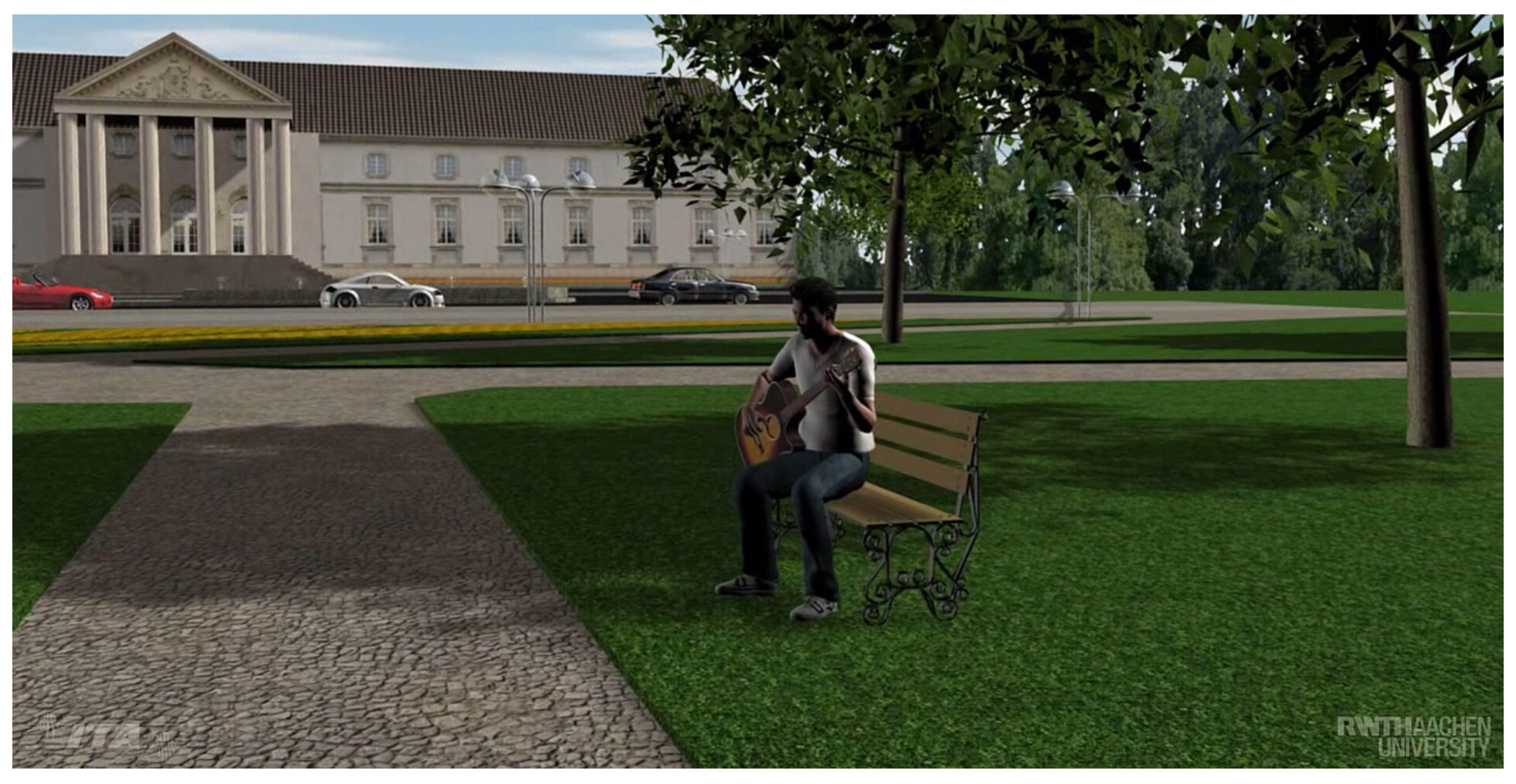
It is also not uncommon today to use geometrical acoustics software for the prediction of sound propagation in outdoor scenarios. Room acoustics parameters are not of interest anymore, but the sound pressure level predictions is a useful indicator. In recent years, the idea of soundscapes gained popularity, aiming at urban sound design and concerning the health problems caused by noise. The presented acoustics library has been used on several occasions in the past to auralize outdoor sound scenes, an example which included video rendering is shown in Figure 14.

Figure 14. Auralization of a dynamic outdoor scene. The RAVEN library was used to produce spatial 3D sound for multiple sources, such as cars, a guitar player, birds, etc.

Figure 14. Auralization of a dynamic outdoor scene. The RAVEN library was used to produce spatial 3D sound for multiple sources, such as cars, a guitar player, birds, etc.

4.2. Supporting Architectural Design

Next to the acoustical planning done by acoutic consultants, the plug-in can directly used by an architect during the design process of a building. For example in the early design stage which is very critical because fundamentals of a construction are defined here. In this phase, without an acoustic consultant being involved (yet), irreversible acoustical design mistakes might occur. Using the plug-in such mistakes can be avoided by investigating the acoustic impression and the effects (e.g., of material compositions and room shapes) in an experimental and intuitive way.

Figure 9 (see Section 3.4) shows an actual example of a contribution prepared for an archictural design competition for an opera house (Work by Alessia Milo and Fabian Knauber for the Student Design Competition (Newman Fund) judged at the International Congress on Acoustics (ICA) 2013 in Montreal). The SketchUp plug-in was used during the design process to monitor and control room acoustics parameters for three different use cases, which were supported using variable room acoustics through movable panels.

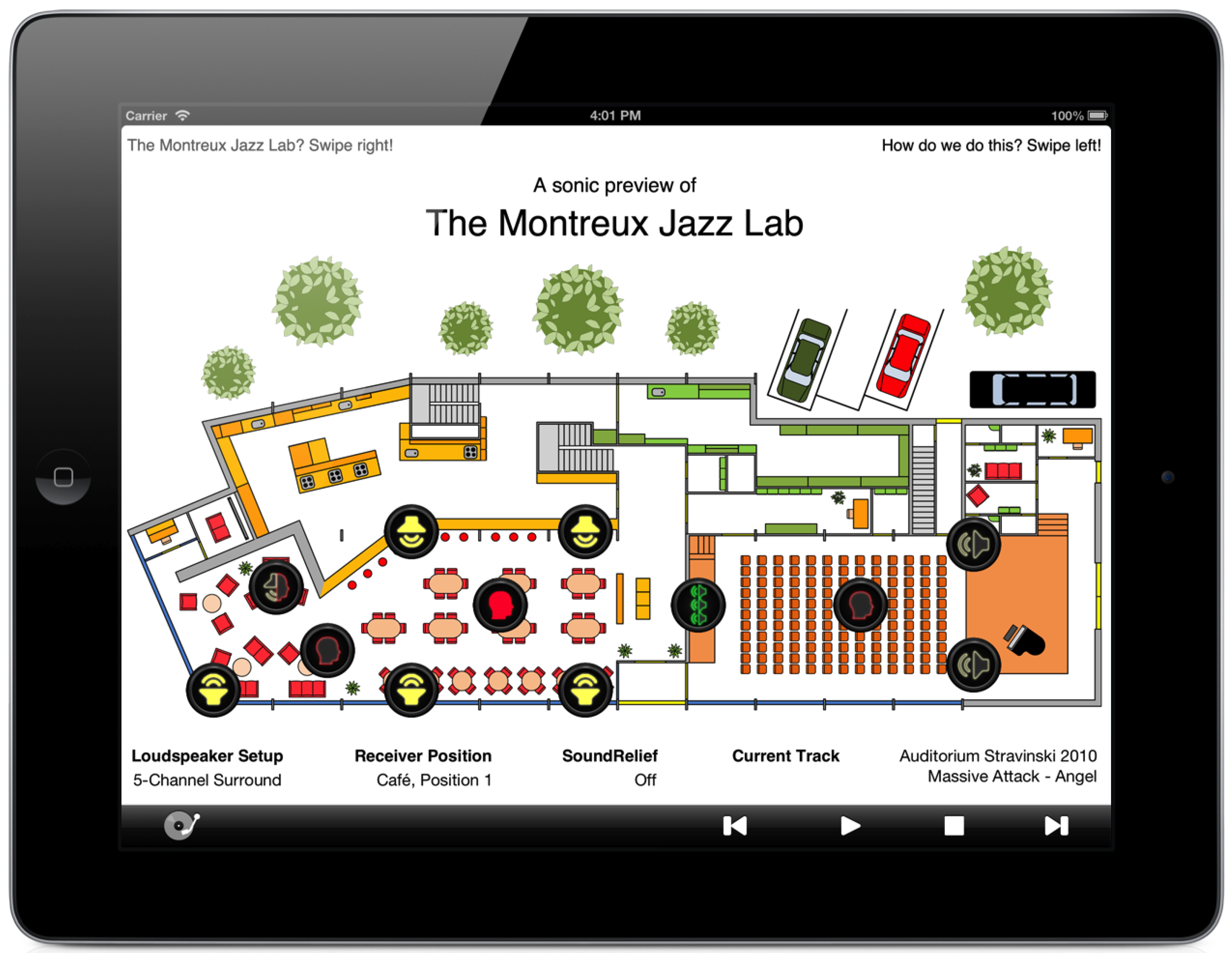
Besides controlling and optimizing the room acoustics already in the early planning phase of buildings, the auralization framework is perfectly qualified to present design results to clients and the public in an imposing and natural way. An example for this is the first sonic preview of the Montreux Jazz Lab (opening in 2015), which was exhibited at the Montreux Jazz Festival in 2013. The Montreux Jazz Lab will be built on the EPFL campus and offer the public the opportunity to discover and relive the Montreux Jazz Festival archives. This outstanding archive, which lately had been given UNESCO heritage status, comprises over 5000 h of video and audio recordings from more than 4000 concerts of renowned musicians. Virtual concerts at different positions in the virtual Montreux Jazz Lab can be auralizted using an iPad application, as shown in Figure 15. The implementation makes use of the SUC to interface between the SketchUp and its auralization module with the tablet as an external controller.

Figure 15. Tablet application for playback of recordings from the Montreux Jazz Archives in the virtual Montreux Jazz Lab. It remotely controls the auralization through an SUC module.

Figure 15. Tablet application for playback of recordings from the Montreux Jazz Archives in the virtual Montreux Jazz Lab. It remotely controls the auralization through an SUC module.

4.3. Teaching Room Acoustics

A strong application of the presented plug-in simulation was found in education. The tool makes it very easy to demonstrate the effect of architectural decisions on the resulting acoustics conditions. While primarily used in architectural and acoustics teaching the visualization plus auralization concept may be well placed in civil engineering, sound engineering and music courses, too. No technical background is necessary to listen and understand or even demonstrate the effects of different rooms, source directivities, receiver positions, etc. The easy access of the software makes a short tutorial sufficient to get started. This factor also led to the practice to include hands-on sessions into the courses during which every student will operate the software on an own laptop. It was observed that this learning model is well accepted by the participating students. The software bundle of SketchUp, SUV and SUA is successfully being used in university courses in different countries around the world (It is freely available upon request. Please contact the authors.) and is regularly demonstrated at various occasions and conferences. In the courses, the students are operating in SketchUp with the SUV and SUA modules running in the background. After around 30–60 min, the participants are usually able to work with interactive auralizations and require only minimal help from the instructor, in some cases even no help at all. At demonstrations and courses especially people with little experience in room acoustics are impressed by the interactive operation and the real-time sound output. The plug-in turned out to be a useful tool to rise awareness and understanding for room acoustics and spatial hearing.

4.4. Sound Reinforcement Systems

A typical use case for available room acoustics simulators is the calculation of sound pressure levels in sound reinforcement applications. Many loudspeaker manufacturers use simplified models to account for the room influence which may provide only very rough approximations especially for exceptional rooms. As the presented plug-in provides room acoustics prediction including processing of directional data of loudspeakers, it has the potential to be used for detailed planning of sound reinforcement systems, ranging from complex announcement installations to live concert public address systems.

4.5. Music and Sound Production

A completely different application is found in sound engineering, e.g., in music production or movie post-production. In the process of multi-track mixing, an important step deals with the spatial placement of instruments. Up to now this is limited to the production of stereo mixes, which uses simple amplitude panning between two loudspeakers. The ambitious engineer, however, often tries to give depth and a distance impression to elements of the mix. This is usually done by balancing direct-to-reverberance ratios and adjustments to the delay between direct sound and randomly set early reflections. This process is much facilitated by employing the room acoustics auralization module, with a simple stereo microphone pattern used as receiver directivity (provided in the library). Natural reverberation and spatial coding including offset in depth are easily arranged and realistic sounding.

To integrate the binaural/spatial production in music processing, the SUA module was compiled as an experimental beta version for the widely used VST (Virtual Studio Technology by Steinberg architectures. VST plug-ins are a worldwide standard for integration of signal processing elements into Digital Audio Workstations (DAWs). An SUA-VST instance can easily be plugged into the signal chain of an audio channel in the DAW and thus smoothly integrates into the mixing engineer’s workflow. Each channel is then represented by a sound source in the SketchUp scene view, which allows direct and intuitive modification of spatial placement and reverberation adjustments through room modeling.

4.6. Export to Virtual Reality Systems

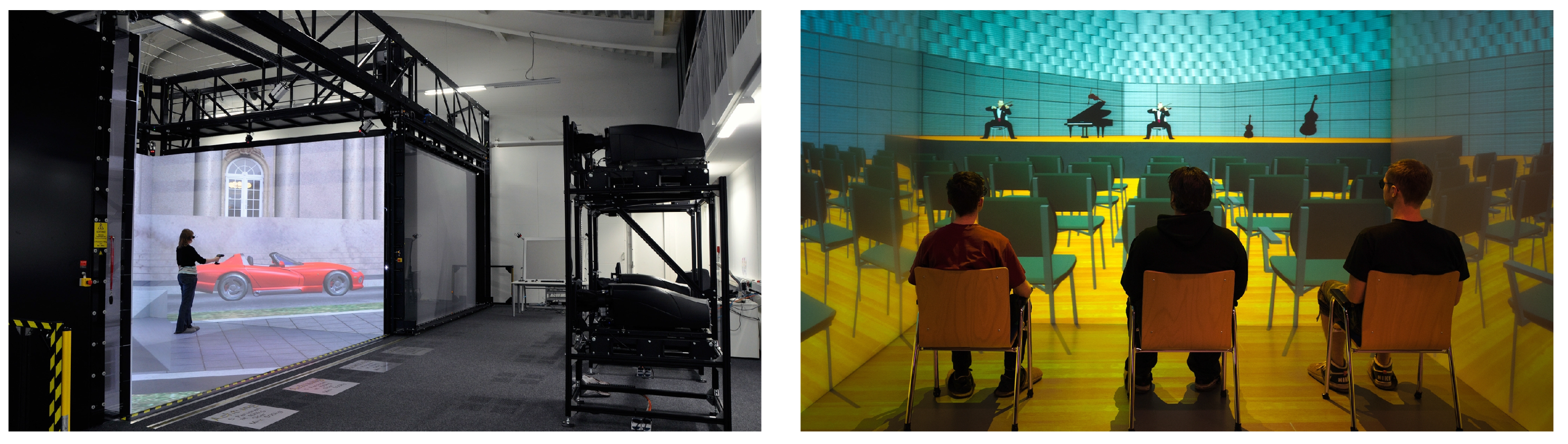
Another field of application are virtual reality systems, which aim at representing reality and its physical attributes in an interactive computer-generated virtual environment. Especially in architectural applications such as a virtual walk through a complex of buildings, auditory information helps to assign meaning to visual information. Today, top-class systems, such as immersive CAVE systems (see Figure 16), enable an all embracing multi-modal experience with a strong feeling of presence for the user. But also less expensive systems, such as stereoscopic beamers, high-resolution TV screens or virtual reality headsets in combination with a 3D audiovisual rendering system and a few of-the-shelf PCs, are already capable of presenting a quite realistic image of the simulated scene.

Figure 16. Virtual attendance of a concert in a simulated concert hall using the AixCAVE at RWTH Aachen University.

Figure 16. Virtual attendance of a concert in a simulated concert hall using the AixCAVE at RWTH Aachen University.

As for the visual representation, the most promising low-budget system is probably the Oculus Rift, which is a next-generation virtual reality headset designed for immersive gaming. The headset features an HD screen and uses a combination of 3-axis gyros, accelerometers and magnetometers for a precise and fast tracking of head-movements (1000 Hz refresh rate). Such a device can easily be integrated into the workflow of SketchUp and SUA by mapping the visual output to the Oculus Rift and sending the Oculus’ head-tracking data to the SUA auralization module via an SUC.

5. Conclusions and Outlook

This paper describes state-of-the art methods for the prediction of room acoustics. These base on geometrical construction of reflection paths. With a hybrid image sources and ray tracing method two very popular and validated algorithms were used for the implementation of a room acoustics simulation library in C++, called RAVEN. The library was used to develop two modules for visualization (SUV) and auralization (SUA) of room acoustics. The main feature of RAVEN is the capability to work in real-time environments and return nearly instant responses to simulation requests. The performance was maximized by code optimization and parallel processing through multi-threading. Also the distribution across multiple computers is available due to TCP/IP interfaces between all modules. The real-time features are accessible through these interfaces and were used to connect the library to a plug-in that was integrated into the popular 3D modeling software Trimble SketchUp. The plug-in extends the functionality of the 3D editor to include real-time acoustics processing. Acoustics control elements are seamlessly aligned in the SketchUp GUI along with its internal tools and menus. Important room acoustical parameters are visualized directly inside the 3D model view window and are updated at real-time rates while the user works on the room model. Additionally the sound card is used to play 3D sound including reverberation that is calculated by the room acoustics library. The real-time in-place result visualization and audio feedback together with the seamlessly integrated controls of the plug-in provide a highly intuitive workflow and interactivity.

The resulting package forms a very versatile tool that attracts many users. Architects, acoustic consultants, as well as teachers, students and also sound engineers belong to the group of actual and potential users. By directly plugging into the 3D modeler the acoustics module integrates well into the workflow of an architect, who is able to run simulations without a deeper founded knowledge in acoustics and without being an expert user of the usually complex simulation programs. But the low entry level of the chosen software SketchUp also enables acoustic consultants and other people unfamiliar with 3D modeling to effectively work on their acoustic models. The real-time plug-in has many applications, with some of them being outlined in this paper. They range from architectural design and acoustical planning over very successful examples in education up to artistic use in sound production.

For the future it is planned to develop a base class for the plug-in on the 3D modeler side, so that implementations for different 3D editing software is easier to derive. This base class could be written in Python or C++ to support many of the popular modelers. However due to the different internal structures of these programs a lot of work has to be spent on the final implementation and maintenance. Another feature that is missing in the current implementation is a convenient export option for the results of the visualization which would be useful for documentation and further evaluation.