Synthesis of a Virtual Urban Soundscape

Abstract

The main research question addressed in this article is to find out to what extent it is possible to predict statistical noise levels such as L₅ and L₉₅ on an urban public square, based on the information about the square’s functionality, the activities going on, and the architecture of the surrounding buildings. The same information is also exploited to auralize the soundscape on the virtual square, in order to assess the disturbance perceived by people of the traffic noise by means of laboratory listening tests, which are based on binaural sound recordings acquired in situ and incorporated in simulations to evoke typical acoustical situations. Auralizations were carried out by two calculation algorithms (ray-tracing and image source method) and two acoustic scenarios (an anechoic situation and a virtually reconstructed square in Odeon^®). The statistical noise levels, calculated from the auralized soundscapes, compare well with measurements in situ. The listening test results also show that there are significant differences in people’s perception of traffic noise, depending on their origin.

1. Introduction

Virtual sound synthesis has already been applied in various applications [1] (Bianchini and Cipriani 1998). Besides virtual reality simulations [2], 3D play back systems and computer game development, the use of virtual acoustic scenario simulations has evolved to a common practice tool for research in musical and room acoustics [3,4,5]. Recently, auralization [6] has found its place also in hearing research [7,8,9,10], and universal design [11]. In view of applications of virtual acoustics for soundscape assessment in the framework of urban planning [12,13,14,15], one question is how realistic virtual acoustics succeeds to mimic the soundscape in an urban public place, and how adequate appreciations of the sonic environment can be made on the basis of laboratory listening tests, in comparison with surveys.

Most of the studies about soundscapes deal with both objective and subjective aspects. Objective assessments are typically performed by means of noise level measurements, or by more quantitative parameters [16,17]. Subjective aspects have been investigated through surveys in situ or by listening tests based on monaural or binaural recordings [18,19,20].

During the last decade, different assessment methods have been proposed for soundscape research, such as description by semantic differential [21,22], numerical and multidimensional descriptors [17,23], automatic classification method [22,24,25]. Recently, Thorne and Shepherd [26] have prepared a proposal for legislation based on the concept of “quietness” as an “environmental value” in terms of amenity and wellbeing.

Adams et al., Pheasant et al. and Yu and Kanga [27,28,29] stated that the subjective interpretation of a soundscape can depend on the given location, its visual appearance, on the type of activities going on, and on the observer’s personal preference and expectations. Emotional dimensions of soundscapes have been investigated by Cain et al. [30], cultural aspects by Farina [31] and effects of social, demographical and behavioral factors on the sound level evaluation in urban open spaces by Yu and Kanga [29].

In subjective assessment, a person is acting as a measuring apparatus, whose judgment cannot be so easily calibrated as a microphone or artificial head Miller [32] has proposed to use the human perception to link soundscape improvement with traditional noise control methods, in an approach that gives priority to sounds heard with undesirable/desirable judgments. In this way subjects identify different sources, which can then be assessed by classical noise control methods.

Dökmeci and Kang [16] concluded that loudness is a more adequate parameter for indoor soundscape assessment than sound pressure levels and A-weighting.

An interesting human-mimicking computational model was proposed by Oldoni et al. [33]. Their method combines a self-organized map of acoustical features with a functional model of auditory attention, giving to the soundscape designer a quick overview of the typical sounds at an investigated location, and allows assessment of the perceptual effects of introducing additional sounds.

Although soundscape assessment is based on an association process that originates in a genetic code or individual cultural background [31], urban planners and decision makers often prefer to work with international descriptors and single number ratings. A priori to an adequate soundscape design in a context of urban planning, it is important to assess the reliability of predicted acoustic parameters.

In contrast with room acoustics, where the main aim is to understand the impact of the volume, shape and acoustic properties of surrounding structures (such as their absorption and scattering) on the room acoustic parameters (reverberation time, clarity, sound pressure level distribution, speech intelligibility, etc.), in an acoustic assessment of an urban public space the focus lies on determining the impact of the distribution of sound sources, and on their spectral and temporal characteristics, duration and temporal or permanent presence. Influences of surrounding buildings are also relevant, but rather in relation to their function and to the activities that might occur in the buildings or in their proximity.

The main goal of this article is to find out how precisely it is possible to predict statistical noise levels such as L₅ and L₉₅, which not only depend on the overall sound power level of the sound sources and their distance from the receiver, but even more on the temporal features of the stimuli. In the present study statistical values of noise levels are extracted from auralized acoustic scenarios on an urban public square, and people’s perception of these levels are analyzed in different settings.

The feasibility of synthesizing a virtual urban soundscape, based on information about its functionality and the activity occurring in it, is assessed.

In the second part of this paper, laboratory listening tests are performed that investigate the disturbance of two type of traffic noise (stationary traffic noise and traffic noise caused by a clear “sound event”), the influence of the activity of listener to overall disturbance/pleasantness, and the sound pressure level of the noise. The results are analyzed by (Analysis of variance) ANOVA-repeated measures.

2. Methods

2.1. Measurement and Recording Methods

Two kinds of in situ measurements were performed: (1) measurements based on binaural recordings and (2) standard noise level measurements with a certified class “A” sound pressure level meter (Bruel and Kjaer 2236). The recordings were acquired on five randomly chosen positions in the square. Since the recordings were very similar, it was sufficient to choose one (Figure 3b—position 1) for comparison with the simulations. More details about the measurement length and the time of recording are given later in this article.

The binaural recordings were performed by in-ear microphones and an M-Audio^® solid state recorder (Cetacean Research Technology, Washington, DC, USA ) with sampling frequency 44,100 Hz and a dynamic range of 24 bits. The recording system was calibrated in an acoustic laboratory in order to calculate correct absolute sound pressure levels from all recorded samples. The calibration was performed in the diffuse field (reverberant room) at 10 different positions of microphones and one position of omnidirectional point sound source (BK 4295) at three different sound pressure levels 60, 70 and 80 dB. The calibration file used for the analysis of sound pressure levels in 01dB Software was a pink noise recording of 80 dB. The calibration was later double-checked in free field (anechoic room) conditions by placing in-ear microphones on a stand at known distances 4 and 8 m from the same sound source (BK 4295 OmniSource, Bruel & Kjaer, Nærum, Denmark).

The sound analysis of recordings was performed a posteriori, partially in 01dB^®Sonic software, and by homemade Matlab^® routines.

The standard noise level measurements were made simultaneously with the binaural recording using a Bruel and Kjaer 2236 Sound Level Meter with “fast” integration time. These measurements served for double checking the absolute sound levels measured by binaural microphones.

2.2. Simulation Method

The acoustical simulations in this study were performed by ODEON^® prediction software, which uses a hybrid calculation algorithm in which the simulation of the Impulse Response (IR) of a given environment is performed in two steps. The early part of the IR is based on early reflections, which are calculated by combining an Image Source Method (ISM) and Early Scattered Rays (ESR). The late part of the IR, i.e., the part containing late reflections, is calculated by using a Ray Tracing Method (RTM) that includes an advanced scattering algorithm. The length of the first part (of the IR) can be chosen by the software user via the so-called Transition Order (TO). This is the maximum number of image sources taken into account per initial ray. For TO = 0, the simulation is performed with only ray-tracing, which is a very robust calculation method for predicting of acoustic parameters, but which is typically not optimum for binaural auralization of sound. The disadvantage of a large TO, corresponding with a dominant use of the image source method, is that, due to the calculation time increasing exponentially with TO, the simulations become very slowly.

In order to obtain a spatial impression from the simulated space, and to allow listeners to localize virtual sounds, a Binaural Room Impulse Response (BRIR) is needed. In Odeon software, the BRIR at the receiver point is obtained by filtering the calculated room impulse response with the Head-Related Transfer Function (HRTF) for respectively the left and right ear. For this type of approach, the image source method, which is based on calculations in a point, is more convenient than the ray tracing method, which is based on statistics of passing rays in a certain region. In view of this, a moderate TO, with binaural ISM for the early part of the impulse response, and RTM calculations for calculating the less critical later part in a reasonable time, is optimum.

In the two experiments performed in this work we were interested in the accurate prediction of the sound pressure level and statistical noise levels (Experiment 1), and in a high quality auralization of the given soundscape (Experiment 2) respectively. In order to assess the influence of the simulation algorithm on the calculated values and on the auralization quality, simulations with different transition orders, TO = 0, 1 and 2, were performed (further in the text referred to as TO0, TO1 and TO2).

In order to obtain auralized sound for the site of interest the generated BRIRs were convolved with anechoic recordings, recorded in an anechoic room.

2.3. Methods for Noise Analysis

In the analysis, statistical noise level values were used for the objective assessment of noise. In order to be able to describe the most important features of sound level fluctuations, the statistical parameters L₅ and L₉₅ were calculated and analyzed. L_x expresses as the value of sound pressure level that is exceeded during x% of the measuring time.

Another parameter used in this study is the equivalent noise level L_A,eq, which is one of the most frequently used descriptors of environmental noise. L_A,eq,T expresses the level of continuous steady sound within a time interval T, which has the same effective (rms) sound pressure as the measured sound, defined as:

(1)

where p_A is the instantaneous A-weighted rms sound pressure at time t, p₀ = 20 μPa is the reference sound pressure level, T = t₂ − t₁ is the measuring period.

3. Experiments

3.1. Description of the Case Study

The main square of the city of Leuven (“Grote Markt”) was chosen as the site of evaluation (Figure 1). The square is surrounded by buildings such as the town hall, St. Pieter’s church, several restaurants and apartment buildings and has a rich history. Due to many different kinds of sound sources and diverse social activities present in this square on different days and seasons in the year, the soundscapes occurring on this site are quite interesting. The overall most typical sounds occurring on the site are definitely human voices, human steps, bicycles, church bells and busses passing by 10 times per hour during working days. During the past years several changes were made in this square, mainly related to a reduction of its accessibility by cars for reasons of functionality, noise and safety. Nowadays, the square is considered as a pedestrian zone where only city buses are allowed to enter.

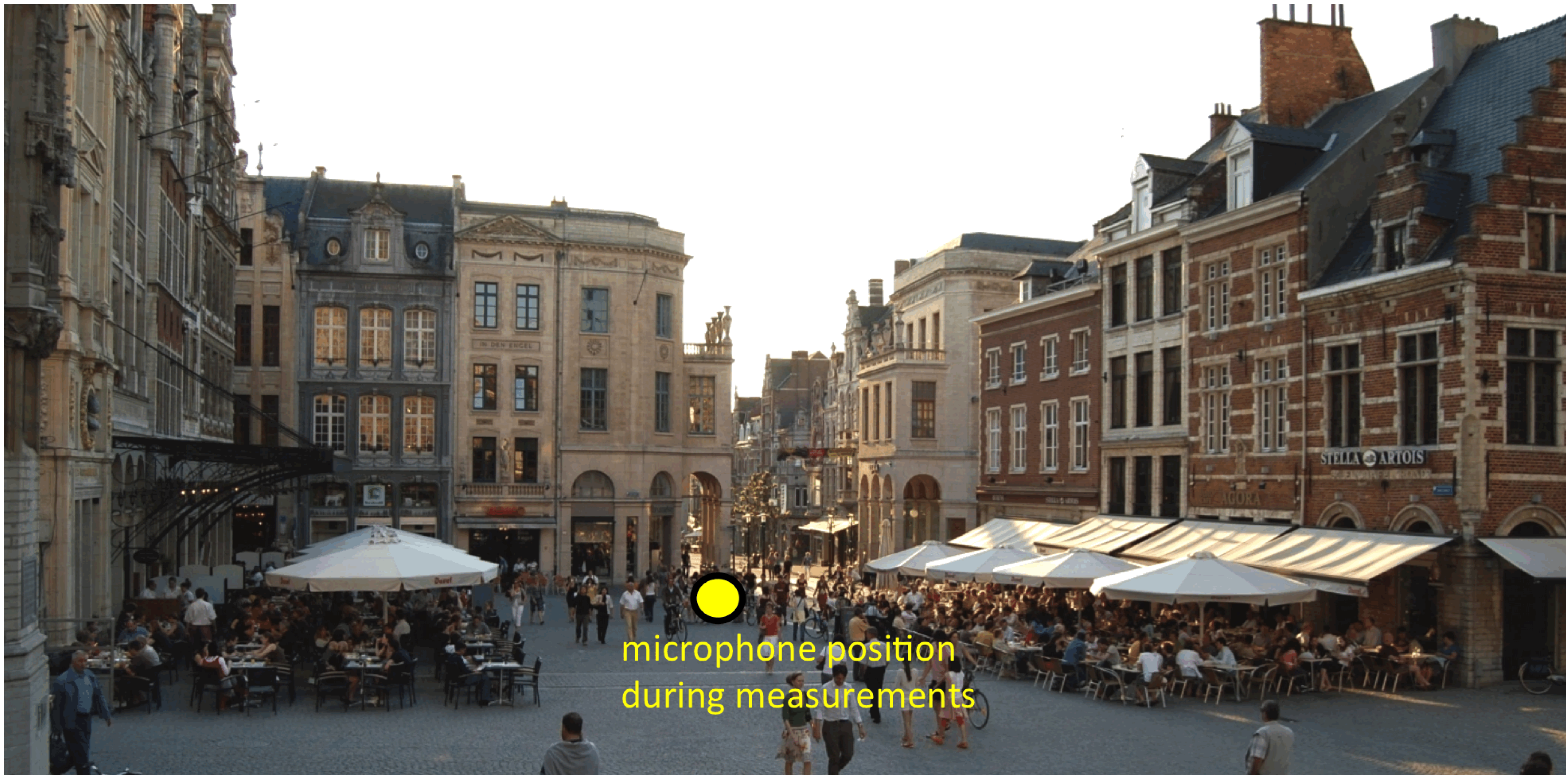
Figure 1. Grote Markt in Leuven, Belgium, view on the part of the square with restaurants with the position of the recording microphone indicated.

Figure 1. Grote Markt in Leuven, Belgium, view on the part of the square with restaurants with the position of the recording microphone indicated.

3.2. Binaural Recordings and Measurements in Situ

Two kinds of recordings were acquired.

(1) A first set of calibrated binaural recordings was acquired in situ by using in-ear microphones (MS-TFB-2 Sound Professionals In-Ear Binaural microphones) and a solid state recorder, on a warm summer evening in the middle of the square surrounded by restaurants full of people. Measurements were done during 15 min on 5 different positions (randomly chosen between two restaurants, about 3–5 m from each other). Since there was not a large difference found between the positions, only one position was taken for comparison with simulations (Figure 1 and Figure 3—position 1). The recordings were performed in a period of the day when no buses were passing in the square, and analyzed in the laboratory in terms of their statistical noise levels and L_eq values.

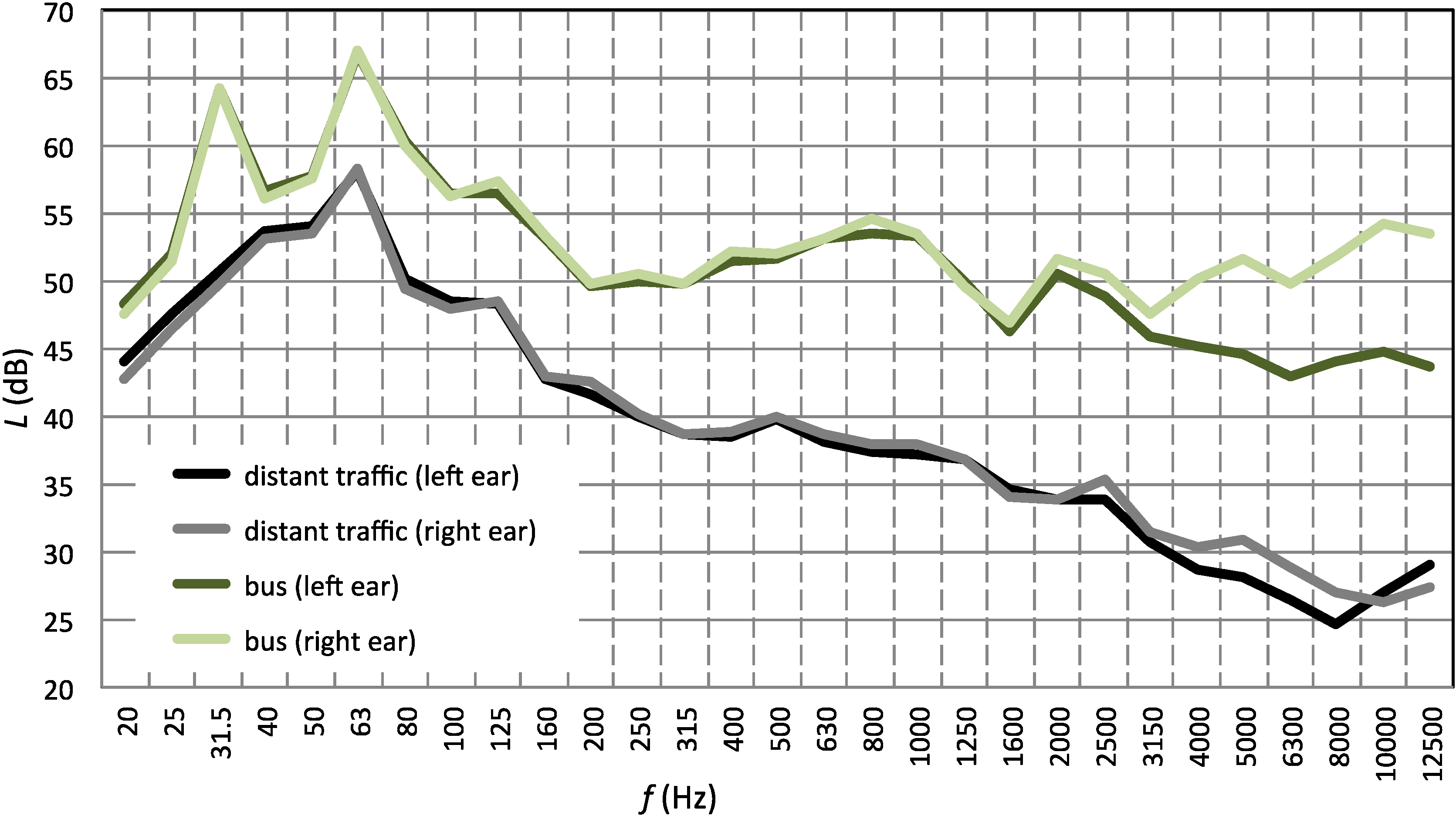
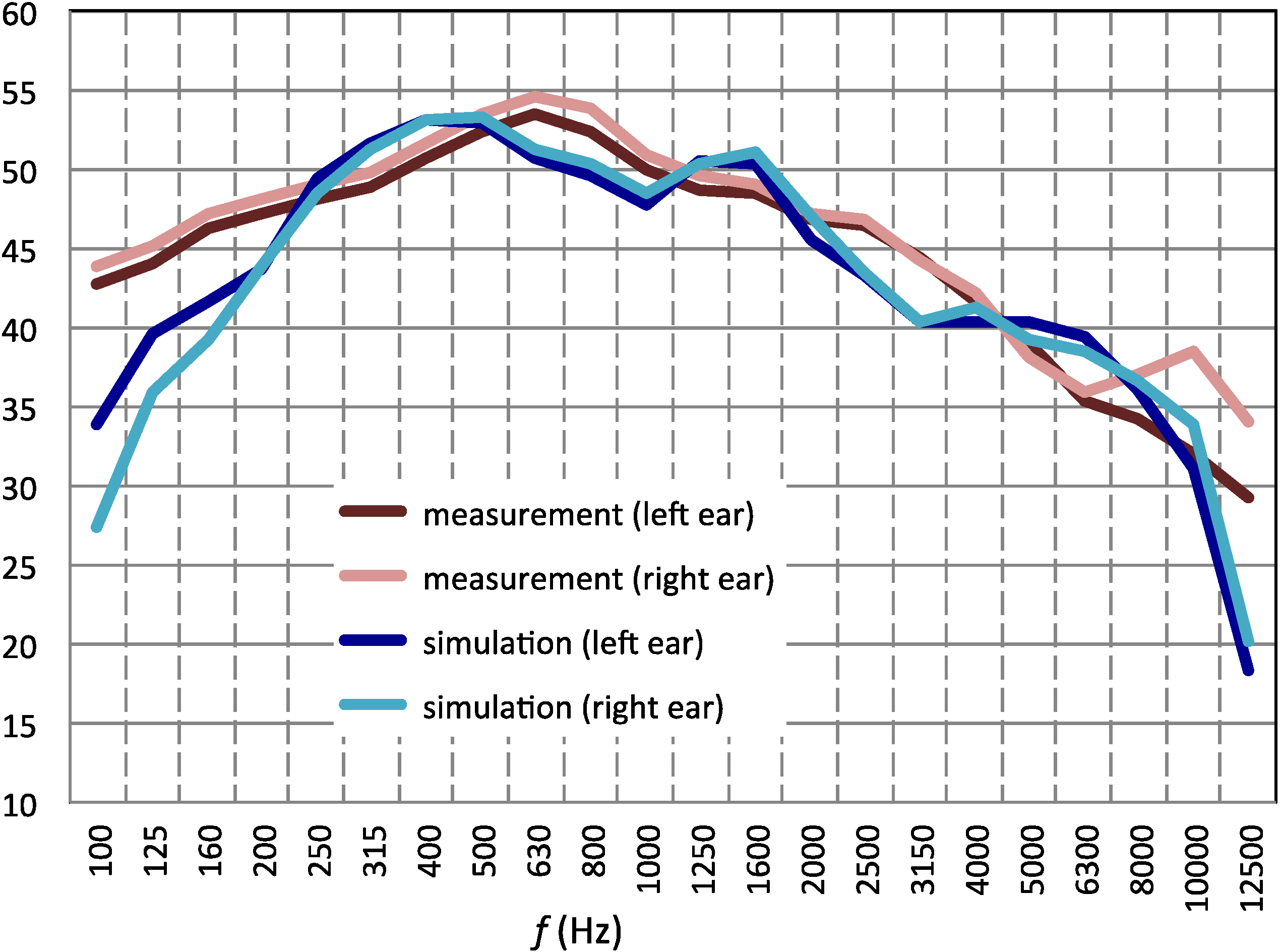
(2) The second set of recordings in situ was not meant for estimation of statistical noise levels, but for the sake of collecting sounds present in the square, which would be very difficult to simulate (due to the Doppler effect on sounds from moving vehicles, etc.), but necessary for later sound synthesis used in the listening test experiments (Experiment 2 of this article). These sounds, e.g., a passing bus and distant stationary traffic noise, were recorded as much as possible individually, during wintertime, when no vocal sounds or birds were present on the square. The frequency spectra of the two mentioned sounds are shown in the Figure 2.

Figure 2. One third of an octave spectrum of distant traffic noise (as measured for left and right ear channel) and a passing bus (as measured for left and right ear channel).

Figure 2. One third of an octave spectrum of distant traffic noise (as measured for left and right ear channel) and a passing bus (as measured for left and right ear channel).

3.3. Recordings in Situ and in the Laboratory

A third set of recordings, of sounds such as different human voices, human steps, various restaurant sounds, e.g., cutlery, glasses, chair movements, etc., necessary for final convolution with simulated BRIRs, were acquired in an anechoic room.

3.4. Acoustic Simulations

A 3D computer model of Grote Markt, Leuven was developed, based on dimensions of the square that were measured in situ by using a laser distance meter and verified by a detailed city plan of the center of Leuven. A simplified spatial model of the square was constructed for the purpose of simulation in Odeon9.2^® software (Figure 3). Grote Markt has an irregular shape but roughly its dimensions can be estimated to 120 m × 32 m. For the sake of making realistic acoustical simulations, parts of the streets that terminate on this square were included in the model, resulting in a total calculation domain of about 240 m × 140 m surface (Figure 3). The sound absorption and scattering coefficients of the surrounding buildings and ground surfaces were estimated based on a visual check in situ.

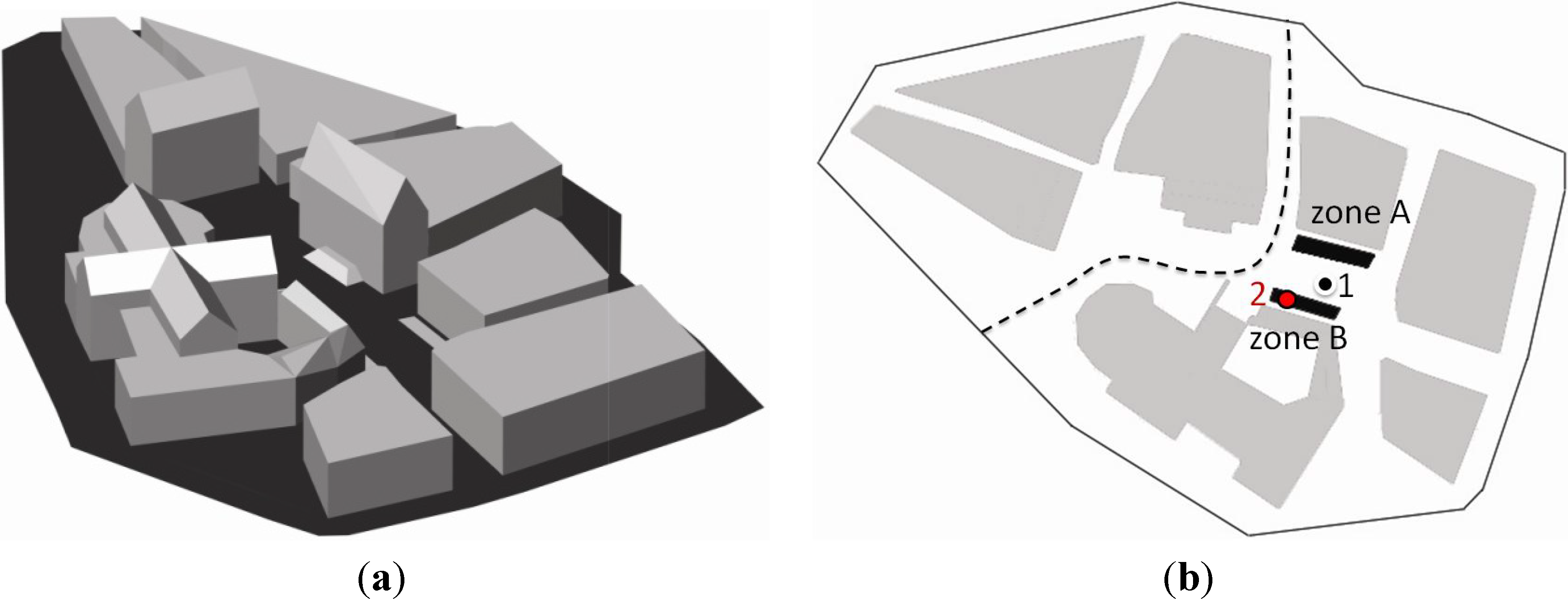
Figure 3. Geometric 3D model of Grote Markt including surrounding buildings (a) and the ground plan of Grote Markt with an indication of the outdoor restaurant zones A and B, and of the two listening positions: 1. in the middle of the square; 2. at the table in the restaurant. The dashed line indicates the trajectory of the buses (b).

Figure 3. Geometric 3D model of Grote Markt including surrounding buildings (a) and the ground plan of Grote Markt with an indication of the outdoor restaurant zones A and B, and of the two listening positions: 1. in the middle of the square; 2. at the table in the restaurant. The dashed line indicates the trajectory of the buses (b).

The acoustic model of the square was closed in a box with boundaries defined as surfaces with a sound absorption coefficient α = 100%, expressing an open-air situation. The BRIRs of the 3D model were obtained from a simulation of a multisource environment with 102 sound sources. Each of the 102 BRIRs was convolved with an appropriate anechoic sample, among which a speaking person, walking people, various restaurant sounds, such as sounds or the cutlery or glass, etc.

These sound sources were regularly distributed into two virtual outdoor restaurant area, in particular Zone A and Zone B (Figure 3b). 58 speaking people were simulated in zone A and 44 in zone B. The auralized samples were mixed to final audio samples (wave files) expressing a summer evening soundscape typical for Grote Markt. The final simulated sound samples were 5 min long, and were analyzed in the same way as the recorded one, i.e., by using the statistical noise analysis.

For the listening tests in the second experiment, shorter sound samples of about 15 s duration, containing the typical features of the simulated soundscape, were prepared.

3.5. Description of the Two Experiments Performed in This Study

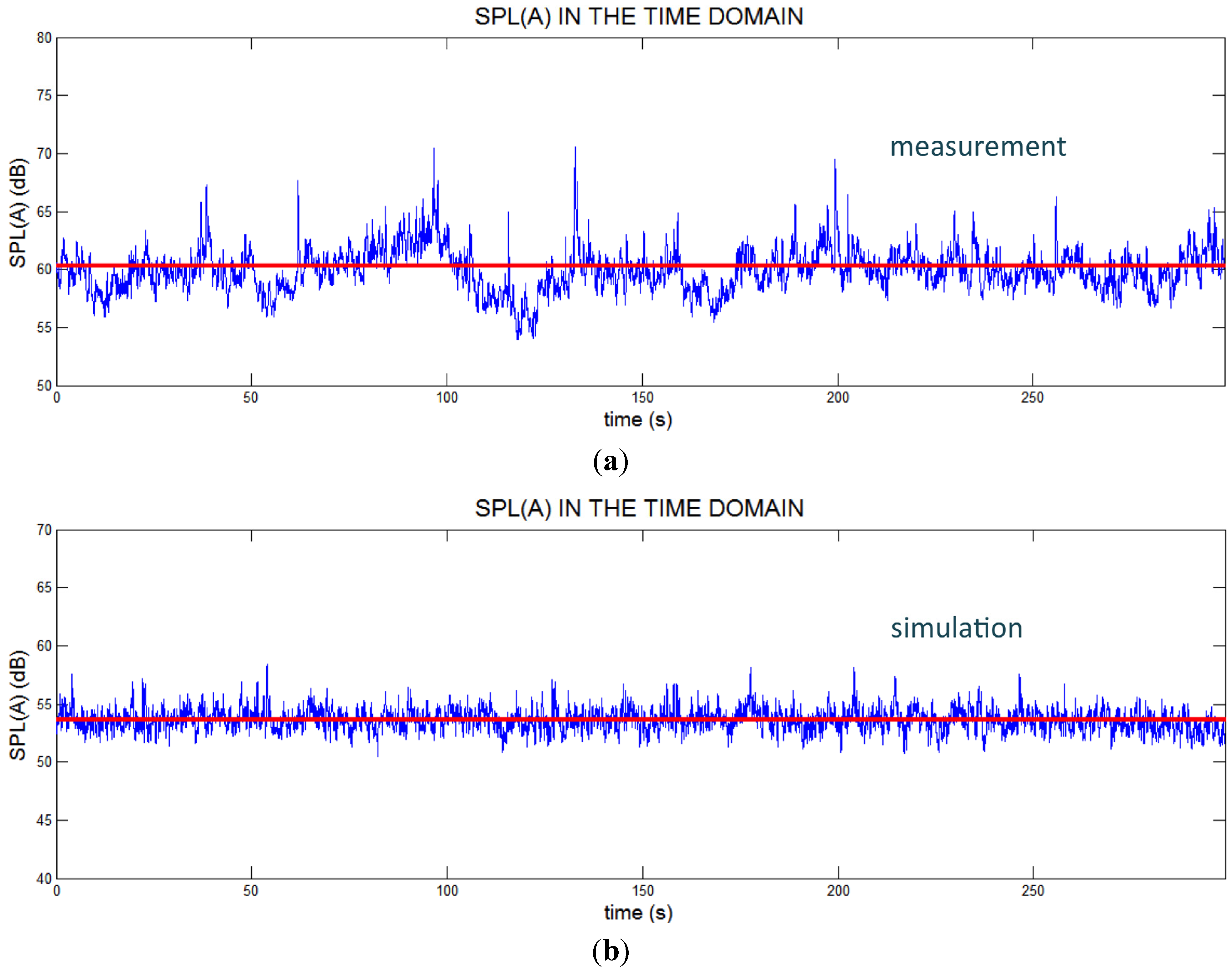
In the first experiment, a comparison was made between the measured and predicted statistical noise levels L₅, L₉₅ and L_Aeq, which were determined for sound samples containing a typical soundscape on the square during evening hours in the summer holiday. Since more than 100 BRIRs needed to be calculated and convolved with anechoic sounds in every considered scenario (TO0, TO1, TO2 and the free field situation), the length of the analyzed samples for comparison with simulation was reduced from 15 min to 5 characteristic min, by cutting a part of the recorded sound out of the in situ recording. The statistical noise levels, the histogram and the spectrum of the selected 5 min fragment were almost identical to the full recording of 15 min.

The simulations for TO0, TO1 and TO2 and for a free field situation were compared with each other and with the measurements (Table 1).

Table 1. Values of L_A,eq for different numbers of speaking people: comparison between simulations and measurements in situ.

Comparison between simulations and measurements	Simulation with TO0		Simulation with TO1		Simulation with TO2		Simulation of free field situation		Measurement
Number of talking people	102	51	102	51	102	51	102	51	>100
LA,eq [dB]	56.8	53.8	56.4	53.6	56.3	51.7	53	51.4	60.3

Table 1. Values of L_A,eq for different numbers of speaking people: comparison between simulations and measurements in situ.

Comparison between simulations and measurements	Simulation with TO0		Simulation with TO1		Simulation with TO2		Simulation of free field situation		Measurement
Number of talking people	102	51	102	51	102	51	102	51	>100
LA,eq [dB]	56.8	53.8	56.4	53.6	56.3	51.7	53	51.4	60.3

Although the prediction of the soundscape in an urban public place is rather difficult, questions from urban planners and decision makers are often related to the prediction of the acoustical situation outdoors and to the proposals of noise reduction or pleasant soundscape creation.

The second, subjective testing experiment was complementary to the objective tests in the first experiment, and meant to verify: (i) if listening tests based on simulated and synthesized sound in the square can be adequately used to verify people’s qualification of elements of a soundscape (such as the sound level, the type of sound); (ii) to assess to what extent the activity of a listener is influencing his or her perception, and to investigate (iii) if synthesized soundscapes could possibly help urban public place developer to estimate the pleasantness of the soundscape.

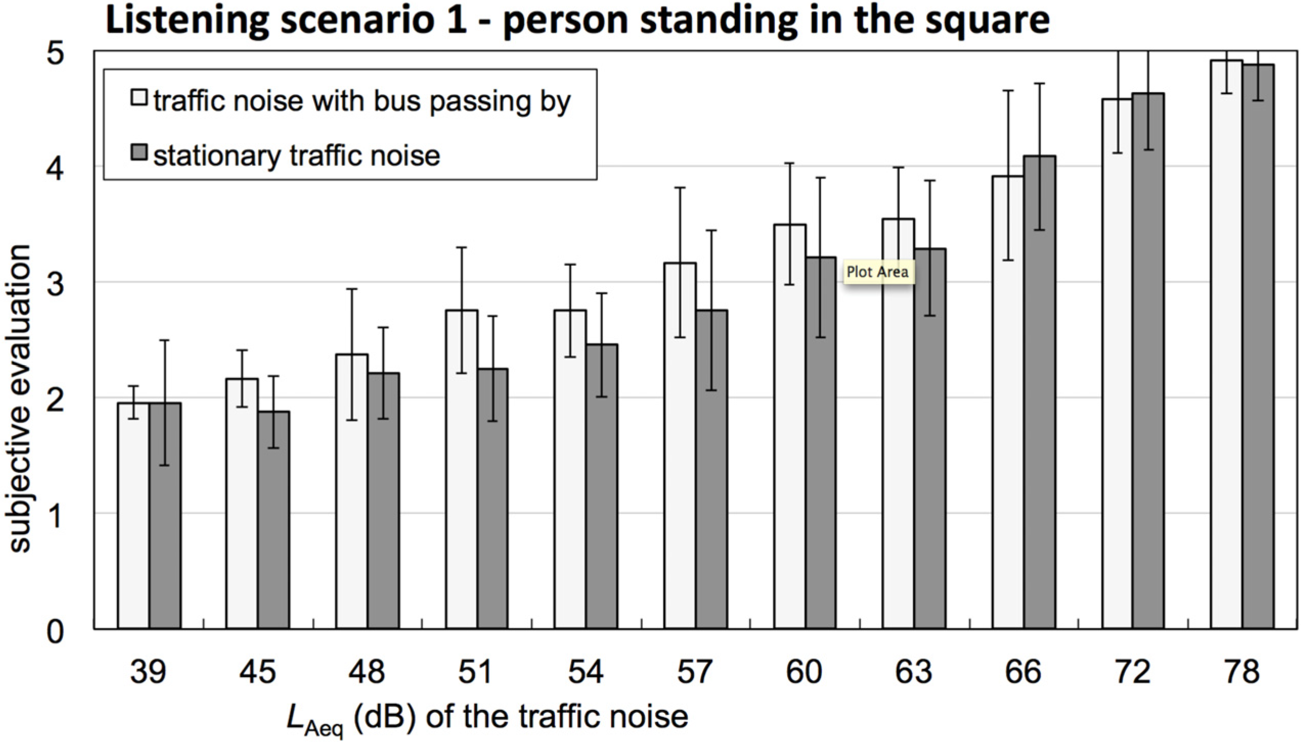
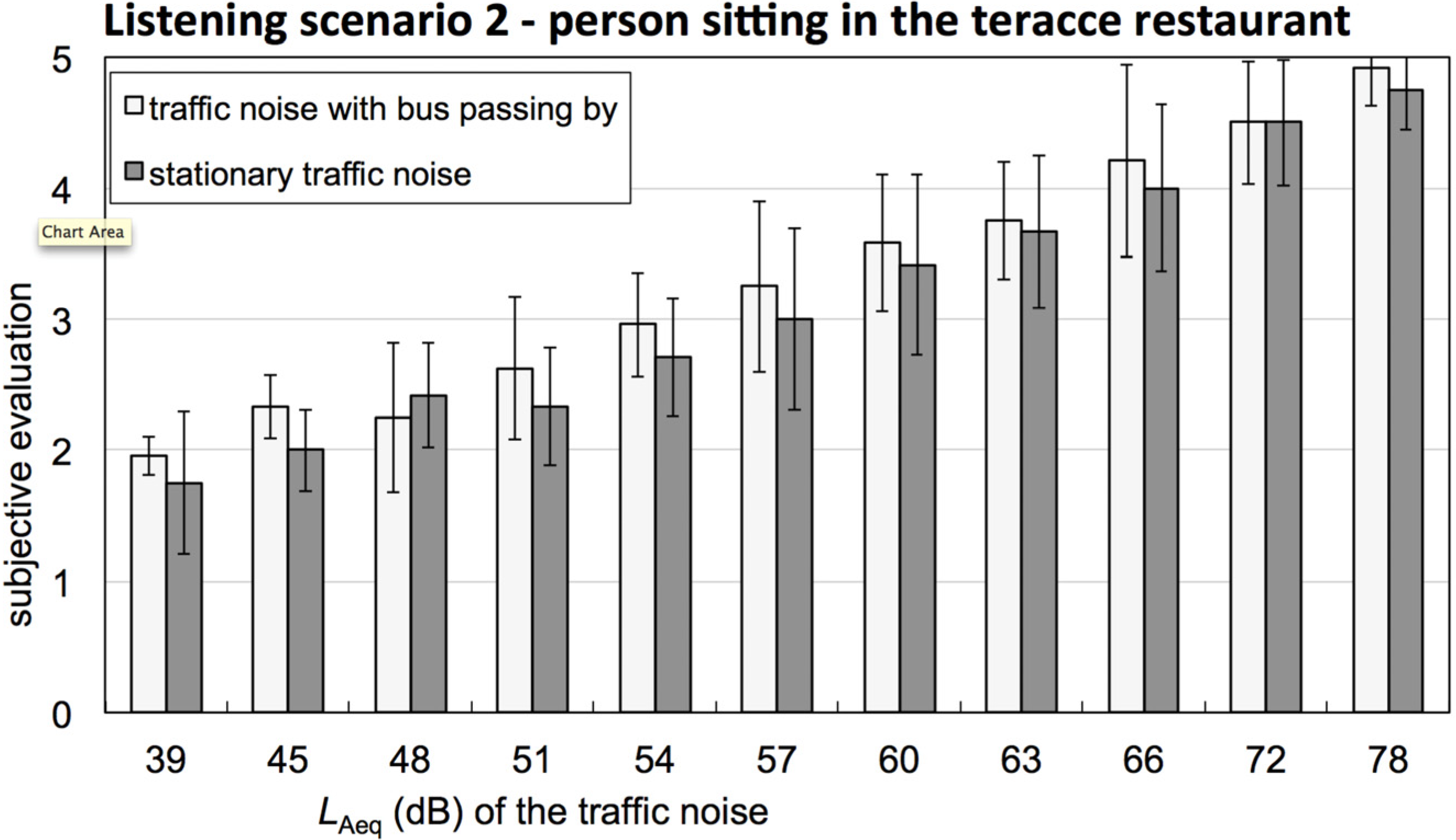
The experiment was based on listening tests that use virtual sound, and investigates the subjective perception of the traffic noise level for two listening scenarios, based on the activity of the person. First, a virtual listener was located in the middle of the square walking between two virtual outdoor restaurants. His or her activity was defined as being waiting for friends (Figure 3b—position 1). In the second simulation, the listener was supposed to sit on the terrace of one of the restaurants, close to the talking people (Figure 3b—position 2). In both scenarios, the sound level of the restaurant sound, i.e., talking people, were constant (at the level of 54 dB (A)). On the other hand, the noise from the traffic was mixed on different sound levels, in order to investigate its disturbing character.

The stimuli played to listening subjects via headphones were created by mixing auralized restaurant sound from the Odeon^® simulation with 22 noise recordings of a different level. Half of them were based on stationary traffic noise recording. The other half contained also the sound of a bus passing by. The reason for the choice of two different traffic noise stimuli was to investigate the different character of noise on perception of an urban soundscape. The first stimulus, stationary traffic noise, is often perceived subconsciously on the background. The second stimulus, a passing bus, was recorded by binaural microphone preserving information about its location, and chosen as a consciously perceived sound.

The stimuli were played in random order to the subjects, each twice. The task of the listening subjects was to imagine him or herself in the sketched situation, and to indicate whether the traffic noise in the given acoustic scenario was (1) too silent; (2) pleasant; (3) acceptable; (4) noisy or (5) disturbing.

Listening tests were performed in the silent anechoic room by using a listening unit of Head Acoustics^® with open headphones. The headphones were calibrated by means of an artificial ear device. The system was calibrated before each listening session.

12 normal hearing listening subjects having an age between 20 and 34 participated in the experiments. The response of each subject was analyzed by means of ANOVA-repeated measures statistics. The number of subjects was large enough for a within subject analysis, which was the main scope of this experiment. Conclusions about the relation between the impact of absolute sound levels on pleasantness/annoyance of the soundscape, which would require a much larger sample of test persons and comparison compared with in situ surveys, were not attempted.

4. Results and Analysis

4.1. Reliability of Objective Quantification of the Synthesized Soundscape on an Urban Public Place

The resulting L_A,eq values, calculated by averaging between left and right ear, are shown in Table 1. The simulated L_A,eq was around 57 dB in all simulations (TO0, TO1 and TO2) , i.e., only 3 dB less than the value observed in the measurement. This difference might be caused by the Lombard effect [34], e.g., the reflex of groups of people, which is related to changes of the characteristics of speech due to a noisy background, in particular in terms of an increase of the vocal intensity, the fundamental frequency, and the word duration. In the simulation, the vocal intensity was presumed as “normal speech” while in reality people might have adopted their vocal output level, e.g., they have spoken louder due to background noise caused by other talking people around. The number of people in restaurant was estimated between 150 and 200. The maximum number of speaking people was estimated at 100 in all simulations, assuming that not more than half of the people present in the square would talk at the same time, as for each talker there is also listener needed.

The predicted value for the free field situation was 53 dB, which is 7 dB lower than the value observed in situ. This shows that the influence of reflections at surfaces of the buildings enclosing the square was about 4 dB.

In the simulated alternatives, in which only 50 people (instead of 100) were talking, a logical drop of 3 dB was observed. In reality the drop in sound level could be expected even larger due to the earlier mentioned Lombard effect.

L₅ was only 58 dB for all simulations, compared to 63 dB in situ, while the simulated L₉₅ value was 55 dB, compared to 52 dB in situ. This can be understood by looking at the dynamics of the sound pressure level fluctuations in more detail. L₅–L₉₅ being 5 dB larger in the measurement than in the simulated soundscape suggests different crowd behavior between the two situations. In the real situation, the speech of the crowd contained slow fluctuations, e.g., 2–5 per minute (Figure 4), independent from the intrinsic fluctuations in speech. Apparently, including random breaks in the speech of every simulated person were partially cancelling out each other, leading to limited fluctuations of the overall sound level. Noise level fluctuations of a talking crowd are probably not completely random. People have a tendency to adapt their speaking level to acoustical and visual circumstances, leading to a degree of collectiveness in the behavior of speech activity and interruption. Comparing the two noise signals in Figure 4 shows that that the fluctuations in a short time period (e.g., 30 s) are very similar between measurement and simulation.

Further analysis of measurement through frequency analysis confirms the dominance of human voices in the square. The spectra of the recorded signals were also found to be more uniform than in the simulated ones, which contained more dominantly speech sound (with dominant frequencies around 400 and 1600 Hz). In a real situation there is more background noise with a rather flat spectrum, which gives a rather frequency independent contribution in the frequency spectrum of real soundscapes. Figure 5 shows the one-third octave spectra for the left and right channel of binaural microphone and results from the simulation.

Figure 4. Comparison of the temporal structure of the measured (a) and simulated (b) sound pressure level in the square.

Figure 4. Comparison of the temporal structure of the measured (a) and simulated (b) sound pressure level in the square.

Figure 5. One third of an octave octave spectrum of the sound as measured in the square for the left (dark red) and right (light red) ear of the binaural microphone and simulated virtual environment for left and (dark blue) and right ear (light blue).

Figure 5. One third of an octave octave spectrum of the sound as measured in the square for the left (dark red) and right (light red) ear of the binaural microphone and simulated virtual environment for left and (dark blue) and right ear (light blue).

4.2. Amplitude Spectrum (in dB(A)) of the Synthesized Soundscape on an Urban Public Place for Determination of Subjective Assessment of Annoyance, Compared with the Measured Spectrum

The result of the second experiment, depicted in Figure 6 and Figure 7, shows people’s perception of traffic noise under two Listening Scenarios (LS), i.e., when standing in the square (LS1), or, when sitting on the terrace of the restaurant in the square (LS2). The grey and white colors in the figures represent the type of noise. Noise type 1 (NT1) in white color is the bus passing by and the Noise type 2 (NT2) in grey color corresponds to stationary traffic noise. 11 different noise levels from 39 dB(A) to 78 dB(A) are plotted along the horizontal axis.

Figure 6. Listening scenario 1: Results given as average values + standard deviation. The subjective evaluation was understood as: 1—too silent, 2—pleasant, 3—acceptable, 4—noisy or 5—disturbing.

Figure 6. Listening scenario 1: Results given as average values + standard deviation. The subjective evaluation was understood as: 1—too silent, 2—pleasant, 3—acceptable, 4—noisy or 5—disturbing.

Figure 7. Listening scenario 2: Results given as average values + standard deviation. The subjective evaluation was defined as: 1—too silent, 2—pleasant, 3—acceptable, 4—noisy or 5—disturbing.

Figure 7. Listening scenario 2: Results given as average values + standard deviation. The subjective evaluation was defined as: 1—too silent, 2—pleasant, 3—acceptable, 4—noisy or 5—disturbing.

Figure 6 and Figure 7 shows that on average people did not perceive any of the stimuli as “too silent”. This is due to the fact that the most silent sample was based on a crowd of people speaking on a level 54 dB (at the listening position), which is not really silent sound. Traffic noise was in both cases perceived as pleasant when its level had reached the same values as the human speech, i.e., values between 50 and 55 dB. Noise levels between 60 and 66 dB were considered as acceptable and impressions of annoyance started around 66–68 dB. Values reaching about 80 dB were found “unbearable” for all the listening subjects.

Statistical analysis in ANOVA-repeated measures gave the following results. No statistical difference was found between the two listening scenarios LS1 and LS2. Apparently there is no difference in perception of the noise level in the square if a person sits in the restaurant or when he/she is waiting in the middle of the square. The absence of effects of a listener’s activity on his or her perception could be caused by the fact that people in the laboratory (in a certain state of mind and without actually being on the square, cannot adequately “imagine” the situation with high precision.

A statistically significant difference of p = 0.002 was found between the two noise stimuli (NT1 and NT2). A passing bus was thus found more disturbing then a stationary traffic noise. This can be caused by the fact that the bus-signal can be geometrically localized (by binaural auditory cues), and also because of the transient temporal structure, evoking a perception as a “noise event”.

Statistical differences were found also between the perception of sounds at different levels (p = 0.013), but not between two neighboring levels, i.e., there was no difference between 48 and 51 dB and 51–54 dB, but levels of 48 and 54 dB were judged differently. Analogously, no difference was found between 51 and 54 dB and 54–57 dB, while the perception of 51 and 57 dB was found to be different.

5. Conclusions

In this study it was verified to what extent statistical values of noise can be used in urban soundscape prediction, for a particular city square scenario. While predicted values of equivalent noise levels were adequate, the prediction of the statistical quantifiers L₅ as well as L₉₅ was less accurate. Apparently, due to effects of collective behavior, slow fluctuations of the speech noise level produced by a real crowd are larger than the ones resulting from rapid random variations of simulated individual talking individuals in the crowd.

A challenge when simulating a crowd people speaking is to estimate the absolute sound levels of voices. There are multiple factors that might influence the vocal output. Besides the distance between talker and listener, which is typically determined by size of the tables in a restaurant, also the Lombard effect can play a role, even in the relatively anechoic conditions of urban public space.

With respect to the perception of traffic noise by a person who is surrounded by people in the square, we found that there is no difference in disturbance by noise depending on the position in the square and the listener’s virtual activity, when the perception test is conducted in an acoustical laboratory. This is in contrast with a number of soundscape studies, which claim that the listener’s activity and visual setting is a key factor in soundscape perception (Viollon et al., 1998) [35]. Apparently, in laboratory tests it is difficult for a listener to “live” the virtual activity so that these kinds of tests can deliver a stronger result when performed “in situ”.

A statistically significant difference in soundscape qualification was found between two different noise stimuli. People perceive stationary noise as “less disturbing” than stimuli containing “noise event” which is also possible to localize. In this experiment a 6 dB difference in noise signal was necessary to obtain statistical significance in assessment of a subjective annoyance.

Finally, situations in which the level of the traffic noise was not stronger than the one of human voices, i.e., 50–55 dB, were considered as pleasant by most of the people, while noise values till 66–68 dB were found acceptable. However these values are only indicative, as more test persons would be necessary for enhances statistical significances.