Integration of Building Information Modeling and Critical Path Method Schedules to Simulate the Impact of Temperature and Humidity at the Project Level

Abstract

Steel construction activities are often undertaken in an environment with limited climate control. Both hot and cold temperatures can physically and psychologically affect construction workers, thus decreasing their productivity. Temperature and humidity are two factors that constantly exert forces on workers and influence their performance and efficiency. Previous studies have established a relationship between labor productivity and temperature and humidity. This research is built on the existing body of knowledge and develops a framework of integrating building information modeling (BIM) with a lower level critical path method (CPM) schedule to simulate the overall impact of temperature and humidity on a healthcare facility’s structural steel installation project in terms of total man hours required to build the project. This research effort utilized historical weather data of four cities across the U.S., with each city having workable seasons year-round and conducted a baseline assessment to test if various project starting dates and locations could significantly impact the project’s schedule performance. It was found that both varied project start dates and locations can significantly contribute to the difference in the man hours required to build the model project and that the project start date and location can have an interaction effect. This study contributes to the overall body of knowledge by providing a framework that can help practitioners better understand the overall impact of a productivity influencing factor at a project level, in order to facilitate better decision making.

1. Introduction and Background

Construction labor productivity is affected by many factors, and weather is one of them; almost 50% of the construction activities are affected by weather [1], including steel construction activities. Both hot and cold temperatures beyond craft workers’ comfort may influence them both psychologically and physiologically and result in productivity losses. As a result of prolonged exposure to freezing or subfreezing working conditions, workers may suffer from health problems such as frostbite, trench foot, and hypothermia [2]. In addition, prolonged exposure to hot working environments may result in psychological effects such as lethargy, irritability, and restlessness, and physiological effects, such as heat stroke, heat cramps, and heat exhaustion, may occur [3]. Occupational Safety and Health Administration(OSHA) sets forth tips regarding how to protect workers from possible health threats because of the cold or heat. One of the common considerations to combat cold and heat is to include more break time into work cycles. Consequently, as craft workers’ tool time (i.e., the time spent on actual work) decreases, productivity decreases accordingly.

Among the climatic factors, temperature and humidity are two of the most critical factors [4] that influence craft workers’ productivity, since they exist ubiquitously and exert their effect on craft workers. Moreover, temperature and humidity have a dynamic effect on construction workers, since the temperature and humidity can vary due to the season and geographical locations. Therefore, starting a project at the different seasons of a year or building a project in different regions of the country can expose the project to different scenarios of temperature and humidity impact.

Nowadays, modern commerce involves retail operations engaging capital project delivery of structures with common construction footprints in multiple geographic locations. Retail stores, such as Wal-Mart, Target, K-Mart, and Home Depot, often build their facilities with a similar building design across the country. A multitude of criteria may be involved in the decision of selecting business locations, such as regional scale of economy, infrastructure, and capital investment. One of the major components of the capital investment can be the costs of buildings. Labor productivity directly correlates with the total costs of a project. Therefore, it is vitally important for a decision maker to understand the impact of factors that affect labor productivity. The goal of this study is to develop a framework to simulate the impact of temperature and humidity on labor productivity at the project level. Understanding the temperature and humidity effect can provide project management with better decisions in project estimating, scheduling, and planning.

2. Literature Review

2.1. Weather Impact

Previous research studies mainly focused on the investigation of the productivity impact of the temperature and humidity at the task level. During the 1970s and 1980s, a number of research studies [4,5,6,7] examined the relationship between labor productivity and temperature and humidity. The National Electrical Contractors Association [5] analyzed the productivity of two electrician journeymen performing the same duplex receptacle installation in an environment where temperature and humidity can be controlled. NECA [5] found that humidity is a significant factor affecting productivity when working at both elevated and low temperatures. Grimm and Wagner [6] performed a study on 51 workers involved in standard masonry wall panel erection and examined the productivity at temperatures 40 to 100 °F with relative humidity 20% to 100%. Koehn and Brown [4,5] performed a similar study by collecting a total of 172 productivity data points, ranging from −40 °F at 90% relative humidity (RH) to 125 °F at 10% RH among steel, masonry, electrical, carpentry, and labor occupations. Thomas and Yiakousmis [7] investigated the relationship between labor productivity and air temperature (with a range of 12 to 82 °F) and humidity (with a range of 18% to 85%). By and large, these models differentiate each other by taking different construction activities and various parameters into consideration, and the productivity data were collected at the different ranges of temperature. Some models collected more data at the warm conditions than cold conditions. However, they all reflect similar trends. Most of the research studies in this area agree on the premise that temperature and humidity have a very influential effect on construction workers’ productivity.

Understanding the temperature and humidity impact on individual tasks is, off course, very important; however, capturing the temperature and humidity effect at the project level is equally important and has been rarely studied. A number of research studies that examined effect of weather on construction productivity at the project level limited their scope to the impact of unworkable conditions, such as precipitations and cold temperatures. For instance, Benjamin and Greenwald [1], Carr [8], Smith and Hancher [9] used different methods and models to simulate the impact of precipitation on construction schedules. Shahin et al. [10] utilized a stochastic weather generator and combined discrete-event with continuous simulation model to simulate weather-sensitive construction activities, such as high-density polyethylene (HDPE) pipe installation. Apipattanavis et al. [11] used a stochastic weather generator to generate probabilistic distribution of weather related variables that could impact construction activities; subsequently weather related delays were estimated through a critical path method (CPM) schedule analysis. Compared to task- or activity-based studies, project-level-based studies allow a better perception of the magnitude of a productivity influencing factor’s impact at the project scale and enable a holistic understanding.

2.2. Building Information Modeling (BIM)

BIM is an emerging technology in the architecture, engineering, construction, and facility management (AEC/FM) industry. Its application covers the whole spectrum of a project’s lifecycle from the conceptual stage to pre-project planning, engineering, construction, operation and maintenance, and decommissioning stage. The adoption of BIM in the AEC/FM industry is on the rise. According to a survey of the Construction Management Association of America [12] conducted in 2007, 35% of the surveyed building owners experienced BIM on some of their projects. In a similar survey conducted by McGraw-Hill Construction [13] in 2012, 44% of the surveyed owners indicated having used BIM on more than 60% of their projects. As the evident benefits of BIM are realized in the industry, coupled with the initiatives made by government agencies and other research institutes, the BIM adoption rate continues to grow. For instance, the office of the chief architect of the General Services Administration’s (GSA)’s Public Building Services (PBS) made BIM mandatory on all new projects undertaken in the fiscal year of 2006 to improve the whole delivery process [14]. Research efforts in BIM execution plan from universities also played a vital part in facilitating BIM implementation in the AEC/FM industry [15].

Because of the versatility of the information contained in a building information model and the interoperability of BIM tools, BIM has its promising application at every stage of a project. A variety of research studies aim to enhance the BIM’s potential uses in various areas. At the conceptual design stage, BIM has been extensively used for sustainability analysis [16,17,18,19] including the aspects of building orientation evaluation, building envelope optimization, daylight analysis, renewable energy alternative evaluation, sustainable material analysis, and site and logistics management; it has also been used for concept-level cost estimation [20]. During the design/pre-construction stage, top three uses of BIM cited by contractors are multi-trade coordination, visualization of design intent, and modeling for constructability evaluation [13]. Lu and Korman [21] performed case studies on two modular construction projects using BIM models, and identified that BIM demonstrates its advantages in design coordination, walk-through animation, and clash detection, particularly in mechanical, electrical, and plumbing (MEP) coordination. To enable exhaustive clash detection in MEP design coordination, Leite et al. [22] identified data items that need to be modeled. Moreover, a number of research studies targeted the utilization of BIM as a platform [23,24,25] for highly automated and intelligent code compliance checking during design stage. BIM also enables automated information queries. Ibrahim and Krawczyk [26] presented an approach in conveying desired CAD objects from an offsite server to the construction site through the web by using extended markup language (XML) to complete the query for the needed data. Nowadays, advancement of cloud computing technology has made model information access, update, and sharing much easier. With regards to the synergies between BIM and facility management, a case study of adopting BIM to set up facility management processes during the construction and turnover phases was performed on the Maryland General Hospital [20]. The findings show that information from different sources stored in the centralized database of BIM on the case project can be successfully integrated with facilities management software, and that early planning is a key to the success. The standard of the Construction Operations Building Information Exchange (COBIE) developed by the Corps of Engineering Research Lab (CERL) plays an important role in the integration of BIM and facility management applications [27].

In the research field, BIM has also been studied for scheduling and planning. Four-dimensional (4D) models (3D + schedule) for construction planning are mostly focused on the visualization of construction processes at the component level of a construction project [28]. Chau et al. [28] broadened the use of 4D model to include site utilization management over the course of construction. While traditional clash detection can only detect clashes between building systems with considering the dynamic change of the construction site, Moon et al. [29] developed an algorithm to generate workspaces and automatically check workspace conflicts with a 4D simulator. Moreover, 4D-based BIM approach is viable for safety check and planning [30,31]. Information provided by BIM cannot completely meet the requirements for on-site project scheduling and management, a framework for an automated and integrated project scheduling and management system was proposed by Chen et al. [32].

3. Point of Departure

This research departs from previous research studies in two directions. First, this research is the first of its kind that examines the impact of the temperature and humidity on labor productivity at the project level. Capturing their overall impact on a project is more of interest to the construction practitioners since the availability of the information could help project management better plan the project. Second, few research studies explored the possibility of using BIM as a platform for productivity simulation studies. This research develops a novel framework that integrates BIM and a lower level CPM schedule to simulate the impact of temperature and humidity on labor productivity at a project level.

4. Objectives and Scope of Research

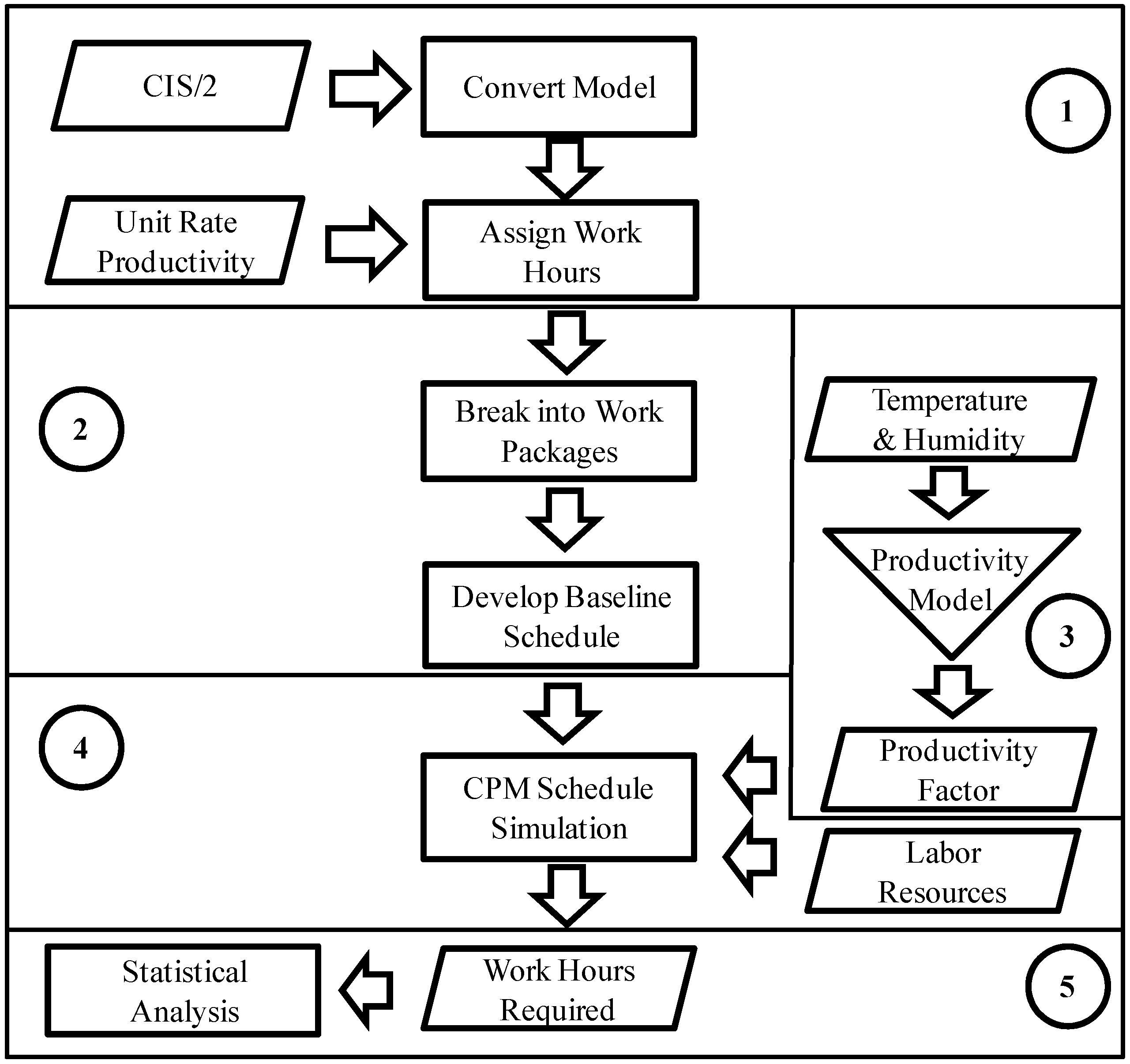
The primary objective of this study is to develop a framework that integrates the building information model with unit rate construction productivity and CPM schedules to simulate the impact of temperature and humidity at a project level. When it comes to decision making for construction projects, historical data can be a good resource. The secondary objective of this study is to use historical weather data from four cities in the U.S. to test how project locations and project start dates at different seasons could affect the project’s schedule performance. The authors readily admit that the other weather factors, such as precipitation, could also affect a project’s schedule. However, precipitation highly depends on the season, geographic characteristics such as mountains, rivers, and topography, and other atmospheric factors. Furthermore, there is not an established relationship between the physical amount of precipitation and construction productivity performance. In order to focus on the impact of temperature and humidity only, the researchers ruled out other factors that could potentially affect construction schedules. This research effort only focuses on the structural steel erection activities of a project due to the following reasons: (1) steel erection activities are undertaken outdoors and subject to the influence of temperature and humidity; (2) the steel activities are the upfront activities, usually given high priority, and less likely to be interfered with by other trades, and thus reduces the noise effect attributed to other factors; (3) structural steel construction usually resides on a project’s critical path and its performance matters the entire project’s schedule; and (4) the BIM standard for steel, CIMsteel Integrated Standards(CIS/2), is a steel trade specific standard with a smaller scope and is easier to implement by most of the software vendors, and thus reduces occurrences of errors during the process of data exchange between different BIM software applications [33].

5. Research Methods

To accomplish the research objectives, this study was undertaken through a workflow shown in Figure 1:

(1)

Convert a CIS/2 formatted building information model obtained from a real project into a virtual construction model (VCM) and assign man hour information to each structural component in the model by referencing a baseline unit rate productivity table;

(2)

Break the VCM into work packages and develop a baseline schedule of the project according to the construction activity sequences that took place on the actual project;

(3)

Obtain historical temperature and humidity data of four selected cities from 1961 to 2010 and calculate mean productivity factor for each day via a selected labor productivity model describing its relation to temperature and humidity;

(4)

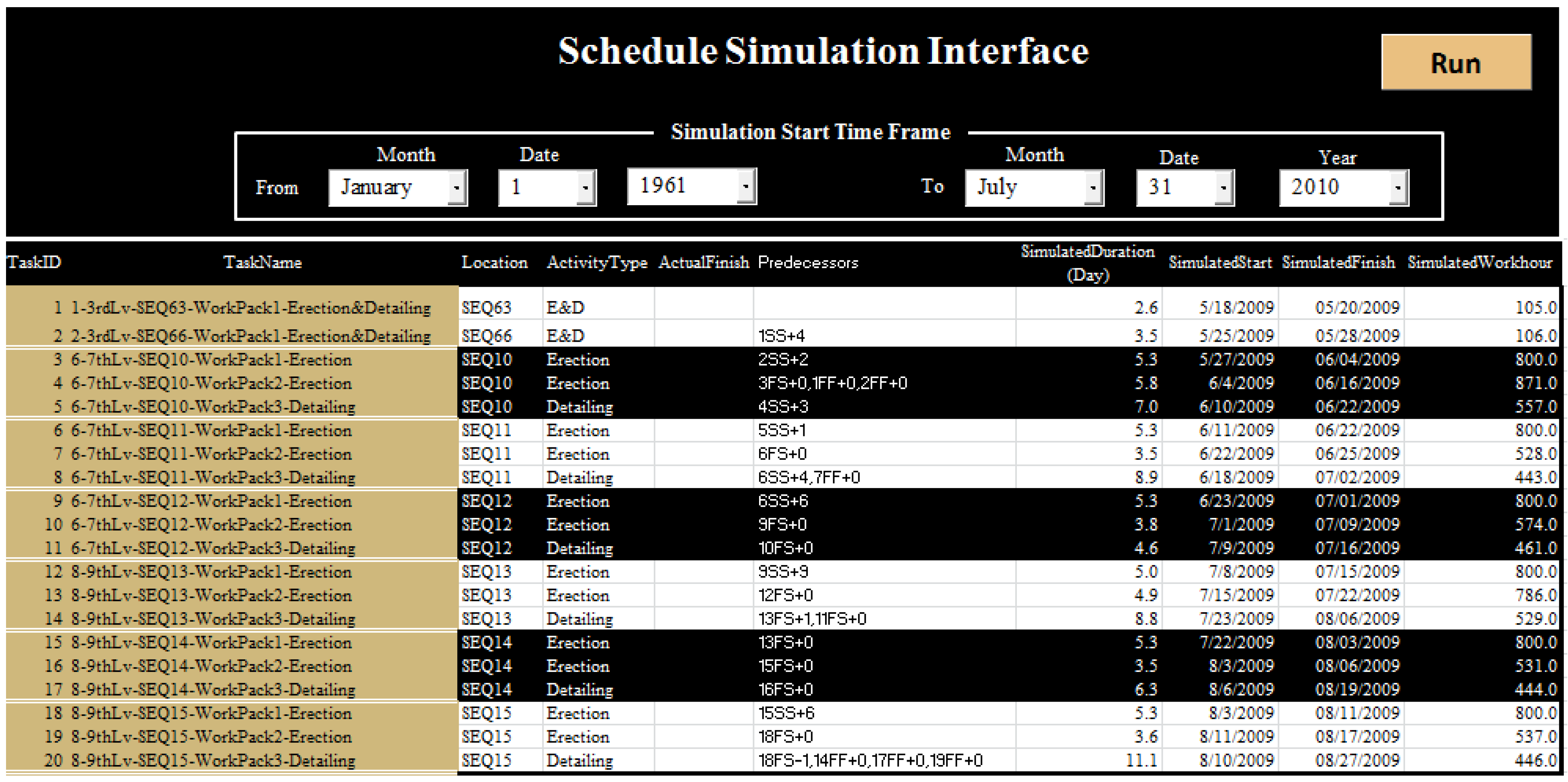
Develop a schedule simulation interface using visual basic for application(VBA) built in Excel to integrate the CPM schedule with manpower sources and productivity factors considering the temperature and humidity effect to automate the process of simulating temperature and humidity effect on the model project;

(5)

Use the simulation interface and input data to generate simulation results in terms of man hours required to build the project under various project locations and project start dates, and perform statistical analyses on the generated simulation results to generate knowledge for decision making.

Figure 1. Workflow of the Research.

Figure 1. Workflow of the Research.

5.1. Why BIM?

BIM plays an important part in this research. BIM was primary used as both a visualization and simulation tool in this research. This research takes advantage of the rich information contained in the building information model and integrates the model with the information of unit rate productivity. This integrated BIM-based scheduling approach allows schedule planners to develop a more realistic and crew level schedule in a more automated manner and reach an accuracy level that might be hardly reached by a traditional way of CPM schedule development. For this study, only one trade was examined. It appears that simple CPM schedule analyses could perform the described study. However, if a model involves multiple trades, developing a schedule with the assistance of BIM integrated with labor productivity would show tremendous benefits. Particularly, for young schedulers, developing a schedule in a BIM environment with 3D graphical representation of the actual building and the man hours associated with model objects can help them better visualize the sequence of the construction activities and properly allocate resources required for each activity.

5.2. Model Project Characteristics

Considering the validity of the research results, the model of the University of Kentucky’s Albert B. Chandler Hospital Pavilion project was used. The entire project started in 2009 and completed in 2011. Turner Construction Company was the construction manager of the project. It has a basement and a five-story podium with two eight-story towers at the top, with a total area of 0.11 million square meters. The complete project has 512 private patient rooms and 28 operating rooms in the surgical suites. The structure of the five-story podium and basement is reinforced concrete. The rest of the structural frame was constructed with structural steel. For this research, only the steel structural model was used.

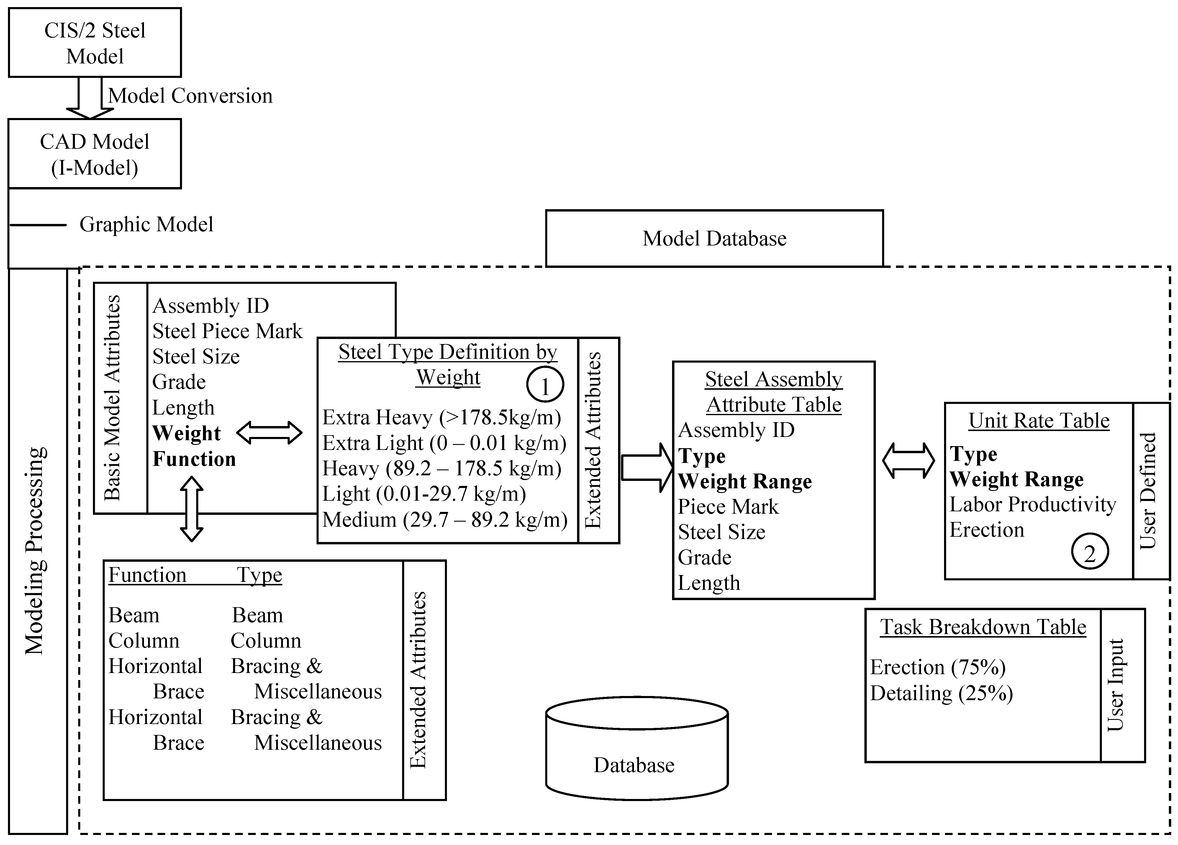
5.3. Virtual Construction Model Processing

The process of the VCM processing is to transfer the information of the engineering model to a BIM application platform and append additional information that complements the construction phase. Figure 2 illustrates the workflow of building a VCM. Two major processes were involved: model conversion and model processing. The purpose of the model conversion is to map the CIS/2 formatted model to a data structure that is unique to BIM software installed on a user’s local machine. This research effort used Bentley’s ConstructSim™ to build the VCM. The model processing is a process of assigning attributes that are related to the construction stage to the model objects. The model processing involved assigning the man hour information to individual steel members through a series of relational SQL database tables by cross-referencing a baseline unit rate construction productivity table (Figure 2). Consequently, man hours required to install each piece of steel were generated. The steel installation activity was further broken down into two tasks, erection and detailing. Erection includes the activities from unloading material to initial bolt-up, and detailing includes leveling, plumbing, final tightening, welding and quality assurance. Based on the work log of the project, the average time spent on erection accounts for 75% of the total installation time, and detailing accounts for 25% of the time. At the end of modeling processing, the man-hour information required for the erection and detailing of each steel member was populated.

5.4. Source of Unit Rate Labor Productivity

This research utilized unit rate labor productivity information to estimate the man hours required to build the project, which was also the basis for baseline schedule development. Ideally, using a company’s historical productivity data would be preferable. However, construction companies treat their craft productivity data as confidential information. Thus, the unit rate labor productivity information was obtained from Richardson™ Construction Estimating Standards. Richardson™ has a 47-year history and has been recognized as reliable standards for cost estimating in the construction industry [29]. Richardson™ was not originally purposed for productivity studies, but it records the information of unit rate labor productivity. The unit rate productivity described herein is defined as man hours per unit of installed work. A lower measure indicates a better productivity. According to the description of conditions where the productivity data were collected by the Richardson™, the working conditions can be considered as the optimal working conditions [34], and the unit rate productivity can be deemed as standard efficient operation. Any working conditions that deviate from optimums may negatively impact labor productivity.

Figure 2. Mechanism of Model Conversion and Processing within the Building Information Modeling (BIM) Application.

Figure 2. Mechanism of Model Conversion and Processing within the Building Information Modeling (BIM) Application.

The steel members in the model project were categorized into five weight classes [35]: extra light, 0 to 0.01 lbs/ft (0–0.01 kg/m), light 0.01 to 20 lbs/ft (0.01–29.7 kg/m), medium 20 to 60 lbs/ft (29.7–89.2 kg/m), heavy, 60 to 120 lbs/ft (89.2–178.5 kg/m), and extra heavy, >120 lbs/ft (>178.5 kg/m) (shown in ① of Figure 2). The structural steel unit rate productivity table in the BIM software used for the study is categorized according to the unit weight range and function, such as beam, column, and brace and miscellaneous items. However, the unit rate productivity of structural steel in the Richardson™’s cost database is categorized by the size and function of steel members. In order to match the format of the standard steel unit rate productivity table (shown in ② of Figure 2) described in the BIM application used for this study, the research effort transformed the format of the unit rate productivity data obtained from Richardson™ to the format that is consistent with the software application. Table 1 describes the aggregated unit rate productivity table.

Table 1. Aggregated Baseline Unit Rate Productivity Table.

Component Type	Activity	Unit Rate (Man Hours/Ton)	Productivity Factor	Weight Range	Function
STEEL_ASSEMBLY	Erect	18.846	1	Light	Beam
STEEL_ASSEMBLY	Erect	13.672	1	Medium	Beam
STEEL_ASSEMBLY	Erect	11.242	1	Heavy	Beam
STEEL_ASSEMBLY	Erect	8.499	1	Extra Heavy	Beam
STEEL_ASSEMBLY	Erect	30.292	1	Light	Bracing and Miscellaneous
STEEL_ASSEMBLY	Erect	31.079	1	Medium	Bracing and Miscellaneous
STEEL_ASSEMBLY	Erect	30.383	1	Heavy	Bracing and Miscellaneous
STEEL_ASSEMBLY	Erect	30.691	1	Extra Heavy	Bracing and Miscellaneous
STEEL_ASSEMBLY	Erect	25.579	1	Light	Column
STEEL_ASSEMBLY	Erect	16.26	1	Medium	Column
STEEL_ASSEMBLY	Erect	10.851	1	Heavy	Column
STEEL_ASSEMBLY	Erect	6.159	1	Extra Heavy	Column

Table 1. Aggregated Baseline Unit Rate Productivity Table.

Component Type	Activity	Unit Rate (Man Hours/Ton)	Productivity Factor	Weight Range	Function
STEEL_ASSEMBLY	Erect	18.846	1	Light	Beam
STEEL_ASSEMBLY	Erect	13.672	1	Medium	Beam
STEEL_ASSEMBLY	Erect	11.242	1	Heavy	Beam
STEEL_ASSEMBLY	Erect	8.499	1	Extra Heavy	Beam
STEEL_ASSEMBLY	Erect	30.292	1	Light	Bracing and Miscellaneous
STEEL_ASSEMBLY	Erect	31.079	1	Medium	Bracing and Miscellaneous
STEEL_ASSEMBLY	Erect	30.383	1	Heavy	Bracing and Miscellaneous
STEEL_ASSEMBLY	Erect	30.691	1	Extra Heavy	Bracing and Miscellaneous
STEEL_ASSEMBLY	Erect	25.579	1	Light	Column
STEEL_ASSEMBLY	Erect	16.26	1	Medium	Column
STEEL_ASSEMBLY	Erect	10.851	1	Heavy	Column
STEEL_ASSEMBLY	Erect	6.159	1	Extra Heavy	Column

5.5. Selection of Productivity vs. Temperature and Humidity Model

This study was built upon existing knowledge of the relationship between labor productivity and temperature and humidity. In the literature review section, the research effort examined different models that depict the relationship between climate conditions and labor productivity. However for this study, the authors selected a model that suits both cold and hot environments and covered a wide range of temperature conditions. Among the four models, Grimm and Wanger’s [6] model was developed based on the productivity data collected at temperatures from 4.4 to 37.8 °C (40 to 100 °F) with relative humidity of 20% to 100%; Thomas and Yiakoumis’ [7] model has a similar issue as Grimm and Wanger’s model in that the reliability of the model is limited by the range of temperature from −11.1 to 27.7 °C (12 to 82 °F); and NECA’s model only focused on a single activity in electrical trades, where the intensity of the work between electrical installation and structural steel erection may differ. Finally, it was decided decided to use Koehn and Brown’s [4] model in this research to predict labor productivity given a temperature and humidity, since the model was developed based on a larger sample size and considered multiple trades, including the steel trade. The relationship of the productivity factor (as a percent of standard efficient operation) relative to temperature and humidity was tabulated as illustrated in Table 2. The productivity factor was defined as the ratio of labor productivity under optimal conditions to the productivity under a given temperature and humidity, and the value is always less than or equal to 1. It should be noted that the labor productivity is defined as man hours per installed quantity. As shown in Table 2, labor productivity is optimal under temperatures from 10–21 °C (50–70 °F) and humidity does not have any effect on labor productivity. However, excessive humidity has negative effects on labor productivity at both elevated and cold temperatures.

5.6. Selection of Project Locations

One of the objectives of this research is to use the developed framework to test how different temperature and humidity scenarios as a result of geographical location could impact the model project’s performance in terms of man hours required to build the project. The authors assumed that project locations do not affect the structural design of the model project. Four cities were selected, including Lexington, Kentucky; Houston, Texas; Newark, New Jersey; and Long Beach, California. Considering the scope of this study described in Section 4, the following criteria were considered when selecting the four cities:

(1)

Temperature and humidity conditions among the four cities are distinctly different;

(2)

The selected cities are not located in the regions where construction activities are suspended during winter seasons;

(3)

The selected cities are not located in the regions that have a relatively long rainy reason.

The purpose of taking the above criteria into consideration was to control the effect of extreme weather conditions on the project’s schedule. It aimed to eliminate the “noise” effect that would otherwise be introduced into the data.

Table 2. Productivity Factor (as a Percent of Standard Efficient Operation) as Function of Temperature and Relative Humidity. Reprinted with permission from [4]. ASCE 1985 American Society of Civil Engineers.

Temperature (°F/°C)	Relative Humidity (%)
	5	15	25	35	45	55	65	75	85	95
−20/−28.9	0.28	0.27	0.25	0.22	0.18	0.13	0.05	–	–	–
−10/−23.3	0.44	0.43	0.42	0.40	0.38	0.34	0.29	0.21	0.10	–
0/−17.8	0.59	0.58	0.57	0.56	0.54	0.52	0.49	0.44	0.36	0.23
10/−12.2	0.71	0.71	0.70	0.70	0.69	0.67	0.65	0.62	0.58	0.50
20/−6.7	0.81	0.81	0.81	0.81	0.81	0.80	0.79	0.77	0.75	0.71
30/−1.1	0.90	0.90	0.90	0.90	0.90	0.89	0.89	0.89	0.88	0.87
40/4.4	0.96	0.96	0.96	0.96	0.96	0.96	0.96	0.96	0.96	0.96
50/10	1.00	1.00	1.00	1.00	1.00	1.00	1.00	1.00	1.00	1.00
60/15.6	1.00	1.00	1.00	1.00	1.00	1.00	1.00	1.00	1.00	1.00
70/21.1	1.00	1.00	1.00	1.00	1.00	1.00	1.00	1.00	1.00	1.00
80/26.7	1.00	1.00	1.00	1.00	1.00	0.99	0.98	0.96	0.95	0.93
90/32.2	0.95	0.95	0.94	0.93	0.92	0.90	0.88	0.85	0.82	0.78
100/37.8	0.81	0.81	0.80	0.79	0.77	0.74	0.71	0.67	0.61	0.54
110/43.3	0.58	0.58	0.58	0.57	0.55	0.51	0.47	0.41	0.32	0.21
120/48.9	–	0.28	0.28	0.28	0.25	0.21	0.15	0.07	–	–

Table 2. Productivity Factor (as a Percent of Standard Efficient Operation) as Function of Temperature and Relative Humidity. Reprinted with permission from [4]. ASCE 1985 American Society of Civil Engineers.

Temperature (°F/°C)	Relative Humidity (%)
	5	15	25	35	45	55	65	75	85	95
−20/−28.9	0.28	0.27	0.25	0.22	0.18	0.13	0.05	–	–	–
−10/−23.3	0.44	0.43	0.42	0.40	0.38	0.34	0.29	0.21	0.10	–
0/−17.8	0.59	0.58	0.57	0.56	0.54	0.52	0.49	0.44	0.36	0.23
10/−12.2	0.71	0.71	0.70	0.70	0.69	0.67	0.65	0.62	0.58	0.50
20/−6.7	0.81	0.81	0.81	0.81	0.81	0.80	0.79	0.77	0.75	0.71
30/−1.1	0.90	0.90	0.90	0.90	0.90	0.89	0.89	0.89	0.88	0.87
40/4.4	0.96	0.96	0.96	0.96	0.96	0.96	0.96	0.96	0.96	0.96
50/10	1.00	1.00	1.00	1.00	1.00	1.00	1.00	1.00	1.00	1.00
60/15.6	1.00	1.00	1.00	1.00	1.00	1.00	1.00	1.00	1.00	1.00
70/21.1	1.00	1.00	1.00	1.00	1.00	1.00	1.00	1.00	1.00	1.00
80/26.7	1.00	1.00	1.00	1.00	1.00	0.99	0.98	0.96	0.95	0.93
90/32.2	0.95	0.95	0.94	0.93	0.92	0.90	0.88	0.85	0.82	0.78
100/37.8	0.81	0.81	0.80	0.79	0.77	0.74	0.71	0.67	0.61	0.54
110/43.3	0.58	0.58	0.58	0.57	0.55	0.51	0.47	0.41	0.32	0.21
120/48.9	–	0.28	0.28	0.28	0.25	0.21	0.15	0.07	–	–

5.7. Historical Weather Data

To determine the temperature and humidity effect on a project, the authors collected weather data regarding temperature and humidity. The project was assumed to be situated in Lexington, Kentucky; Houston, Texas; Newark, New Jersey; and Long Beach, California. Climatic conditions may fluctuate from year to year. In addition, historical data is a good basis for decision makings. To reduce the variability caused by abnormal years, last 50 years’ historical weather data (from 1961 to 2010) were collected for each of these selected cities. The historical weather data were obtained from Weather Underground [36]. Weather Underground (WU) is a commercial weather service provider founded in 1995 based in Ann Arbor, Michigan, and currently holds global historical weather data from 1948 up to today. Weather data provided by WU are collected in hourly intervals for most of the years, and some recent years’ data are collected with a higher resolution of 15-min intervals. Detailed information includes temperature, dew point, relative humidity, sea level pressure, visibility, wind direction, wind speed, gust speed, and precipitation.

For this study, only temperature and humidity data within the regular working hours was investigated. On the model project, the steel craft workers followed a 4 × 10 working hour schedule, working from 7:00 am to 6:00 pm with a one hour lunch break from Mondays to Thursdays. Temperature data beyond that range were filtered out. Temperature in a day can vary with time. Table 3 shows the historical weather data on 4 March 2009 in Lexington, KY, with temperatures ranging from −3.3 °C (26.1 °F) in the morning to 10 °C (50 °F) in the afternoon.

Table 3. Historical Weather Data on 4 March 2009 in Lexington.

Date	Time	Temperature (°C/°F)	Relative Humidity (%)
3 April 2009	6:54 AM	−3.3/26.1	43
	7:54 AM	−2.8/27	41
	8:54 AM	−2.2/28	41
	9:54 AM	1.7/35.1	34
	10:54 AM	3.9/39	30
	11:54 AM	5/41	28
	12:54 PM	7.2/45	24
	1:54 PM	8.3/46.9	20
	2:54 PM	8.9/48	18
	3:54 PM	10/50	19
	4:54 PM	10/50	19
	5:54 PM	8.9/48	22

Table 3. Historical Weather Data on 4 March 2009 in Lexington.

Date	Time	Temperature (°C/°F)	Relative Humidity (%)
3 April 2009	6:54 AM	−3.3/26.1	43
	7:54 AM	−2.8/27	41
	8:54 AM	−2.2/28	41
	9:54 AM	1.7/35.1	34
	10:54 AM	3.9/39	30
	11:54 AM	5/41	28
	12:54 PM	7.2/45	24
	1:54 PM	8.3/46.9	20
	2:54 PM	8.9/48	18
	3:54 PM	10/50	19
	4:54 PM	10/50	19
	5:54 PM	8.9/48	22

Because of the fluctuating temperatures throughout a day, the productivity factor corresponding to each time point where weather data was collected was computed with reference to the productivity factor relative to temperature and humidity listed in Table 3. Then the average productivity factor during the 10 h is considered as the productivity factor for that specific day. A daily average productivity factor was calculated by utilizing Equation (1):

(1)

where, F_d = the average productivity factor during the daytime; F_ti = the calculated productivity factor at the i^th time point t_i; F_ti+1 = the calculated productivity factor at the (i + 1)^th time point t_i+1.

5.8. Baseline Schedule

5.8.1. Develop Work Packages

Work package is a basic unit for site superintendents to organize daily site activities at the crew level. Depending on the size of the crew, the man hours of a work package can vary from 400 to 1000 on a relatively complex project [37]. The next step of this study is to develop work packages. The practice of work packaging enables construction management to breakdown a complex project into manageable units. Work packages are a key for project management to estimate the materials, and labor costs precisely and make sure that the required resources are available at the right time. A large-scaled project can have hundreds or thousands of work packages. Therefore, a systematic naming convention for work packages is instrumental. A self-explanatory name assigned to each work package and organized in a proper order enables model viewers to identify specific work packages in a timely manner. Therefore, the authors used a combination of floor numbers and predefined sequence numbers as a prefix for a work package. Usually before the construction stage, a steel structure is broken down into a number of sequences and a sequence number is designated to a group of steel components. Once the sequence is established, sequence numbers are referred to among steel fabricators and contractors for scheduling materials fabrication and delivery.

5.8.2. Development of the Baseline Construction Schedule

After work packages were created, a baseline schedule was developed. Since this model project is an already completed project, the creation of the baseline schedule followed the precedence of the actual construction tasks that took place on the actual project. The baseline schedule described herein did not consider the temperature and humidity effect yet. The unit rate productivity obtained from the Richardson™ cost data was collected from the activities that were undertaken under the conditions with optimal temperatures, adequate skilled craft workers, decent material supply, easy site access, and proper supervision, which as a whole can be considered as optimal baseline productivity. On the actual project, thorough clash detection and trade coordination were performed before the actual construction activities took place. Thus, construction rework was greatly reduced. In this research, rework was not counted in the creation of the baseline schedule. Work packages were treated as basic schedule task units, since work packages are also the work units assigned to work crews according to job site practices. Through the process of virtual construction model processing described in Section 5.3, the information for the man hours required for the installation of each steel component was populated in the model. Therefore, each work package included the information of total man hours required for installation. By referring to the manpower log describing the allocation of labor resources recorded by the contractor, the duration for each work package was computed. By referencing the sequences of the activities occurred on the actual project, the baseline schedule at a crew level was developed.

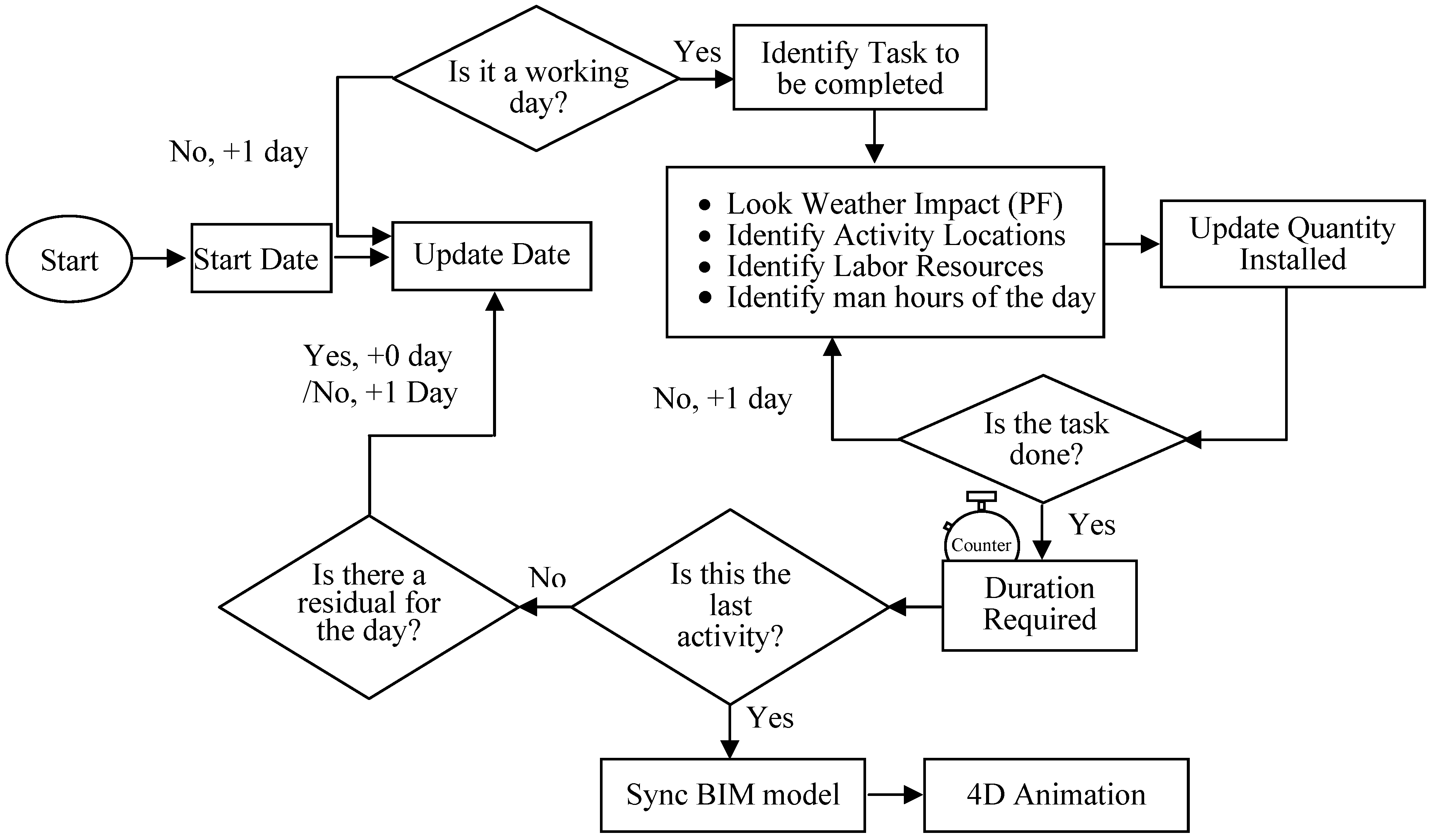
5.9. Algorithm of Schedule Simulation

To automate the process of simulating the effect of temperature and humidity, the researchers developed a schedule simulation interface within the Excel spreadsheet using Visual Basic for Application (VBA) (Figure 3). One of the eminent advantages of BIM is its data interoperability; the work package report can be exported directly from the model database into an Excel spreadsheet, which eliminates manual data reentry. The interested information for the schedule simulation is the work package items and the man hours associated with each work package. The schedule simulation interface was developed based on early start and early finish.

Figure 3. Schedule Simulation Interface.

Figure 3. Schedule Simulation Interface.

The column of “Predecessors” depicts the precedence between the schedule tasks. For example, as shown in Figure 3, Task 6-7thLv-SEQ10-WorkPack2-Erection’s predecessor is listed as “3FS + 0”. In this case, “3” describes the Task ID, “FS” describes the finish-to-start relationship, and “0” denotes the lag between a task’s finish date of and its successor’s start date. In this example, “3FS + 0” indicates that the described task’s predecessor is 6-7thLv-SEQ10-WorkPack1-Erection and that the task starts right after the predecessor finishes. Likewise, SS denotes start-to-start relationship, SF denotes start-to-finish, and FF denotes finish-to-finish relationship. Figure 4 describes the flow chart of the schedule simulation algorithm. For the process of simulation, Fridays, Saturdays, Sundays, and national holidays are assumed as non-work days. Once a start date is picked as the simulation start date, test for working or non-working day test is performed. If the test is false, the next day is picked and the working/non-working day test is repeated. This process is repeated until the test becomes true. If it is a working day, the task to be executed, man hours required for the task, productivity factors, number of workers, and working hours in the that day are identified, so that the quantity installed during that day can be computed. Then another logic test, if the task is completed, is performed. If the task is not finished, the next day is picked. The loop repeats until the task is completed, and the required duration is recorded. Possibly, one task could be completed before the end of day. In this case, the rest of the day could be used to perform the next task. After each task is complete, another test, determining whether the task is the last task of the project or not, is performed. If the test is true, it means the project is completed. The updated schedule considering the effect of temperature and humidity can be synchronized with BIM to perform 4D schedule animation.

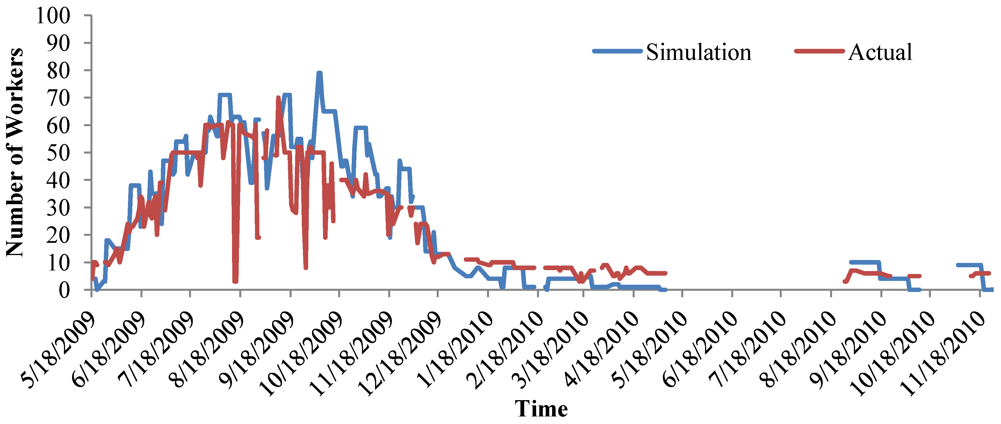
5.10. Model Validation

The model validation process is to test if the built model behaves properly as it is intended. The authors used the developed schedule simulation interface and set the simulation start date the same as the actual project start date, 18 May 2009. Since Lexington, KY is the location of the actual project, Lexington’s historical temperature and humidity data for the years 2009 and 2010 were utilized to compute productivity factors which are the multipliers used to adjust labor productivity, as a result of the effect of temperature and humidity. The simulation process followed a working schedule of 4 × 10 h/week. As mentioned, this research did not take precipitation into consideration. However, the actual project suffered from a number of rainy days and used some weekends and overtime shifts to make up the loss of working days due to sporadic unworkable days. The delays due to precipitation were very minimal and recoverable on the project. The simulated start and finish dates for each work package, and the total man hours required to build the project were generated. As shown in Table 4, the simulated project finish date considering the temperature and humidity effect is 18 November 2010, as opposed to the actual completion date, 23 November 2010. The difference in total man hours required to build the project between simulated and actual results amounts to 518 man hours, which is within 1% of error.

Figure 4. Flow Chart of the Algorithm for Schedule Simulation.

Figure 4. Flow Chart of the Algorithm for Schedule Simulation.

Table 4. Summary of Developed Framework Validation.

Item	Simulation	Actual
Project Start Date	18 May 2009	18 May 2009
Project Finish Date	18 November 2010	23 November 2010
Total Man hours Required	55,465	54,947

Table 4. Summary of Developed Framework Validation.

Item	Simulation	Actual
Project Start Date	18 May 2009	18 May 2009
Project Finish Date	18 November 2010	23 November 2010
Total Man hours Required	55,465	54,947

Figure 5 shows the actual and simulated man-power loading over the whole duration of structural steel installation. Though larger variation is shown at the last quarter of 2009 because of the small amount of rework and overtime presented on the actual project, the overall trends show a large degree of consistency.

Figure 5. Manpower Loading of Simulation vs. Actual Record (Lexington, KY).

Figure 5. Manpower Loading of Simulation vs. Actual Record (Lexington, KY).

The process of validation provides the confidence that the aggregated unit rate productivity obtained from Richardson™’s cost data, selected productivity model, and the developed simulate interface are reliable enough to be used to perform simulation under various scenarios and generate meaningful knowledge against temperature and humidity impacts on a project.

5.11. Schemas

One of the objectives of this research is to use this developed framework to help with project decision making considering temperature and humidity effects. To accomplish this goal, the research effort proposed the following schemas to perform the simulations and statistical analyses on the generated the simulation results.

Four specific dates in a year were picked as the project starting dates for the schedule simulation. The four dates are the first day of the quarters of the year, i.e., 1 January, 1 April, 1 July, and 1 October, which allow the project to have an equal probability of exposure to temperature and humidity changes due to seasons. Fifty years of historical data (from 1961 to 2010) of the four selected cities were downloaded, and the productivity factor for each day of the last 50 years was calculated. Through the schedule simulation interface, the user can specify a period during which a project start date can be picked for simulation start date (Figure 3). As shown in Figure 3, the first run of simulation starts on 1 January 1961, second on 1 April 1961, third on July 1961, and so on and so forth. At the end of simulation, the simulated start and finish dates, and man hours required to build the model project can be automatically computed and stored in the “Output” Excel spreadsheet.

With generated simulation data, the research effort can perform a series of statistical analyses. Among the generated simulation data, interested dependent variable is total man hours required to build the model project. In this analysis, four project start dates and four project locations were involved, which consists of a typical 4 × 4 two-way analysis of variance (ANOVA). Three hypotheses were tested in this study. The null hypotheses are described as follows:

• H1₀: Starting the project on different dates would not change the man hours required to build the project;
• H2₀: Situating the project at different locations would not change the man hours required to build the project; and
• H3₀: The project location and start date would not have an interaction effect on the man hours required to build the model project.

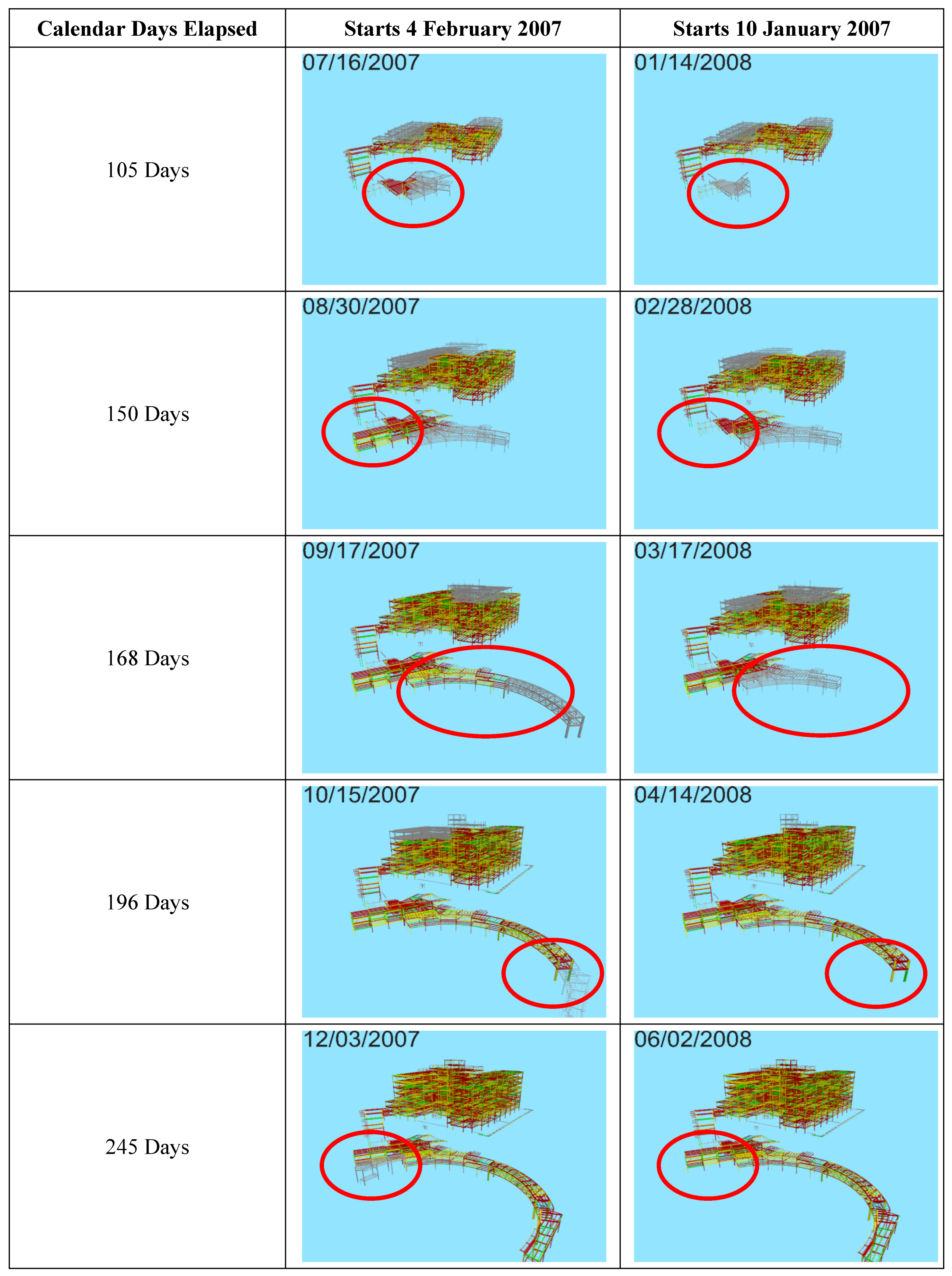
5.12. 4D Schedule Animation

4D schedule animation is usually used to visually present how a building is built and a project’s construction status with respect to a timeline. 4D schedule animation is achieved through linking the model objects with the project schedule. For this study, in order to link the schedule with 3D models automatically, the names of the work packages created in the model match the task names in schedules. To visually compare the schedule performance under two different scenarios in terms of different project locations and/or project start dates, two 4D schedule animations can be played in parallel.

6. Results and Discussion

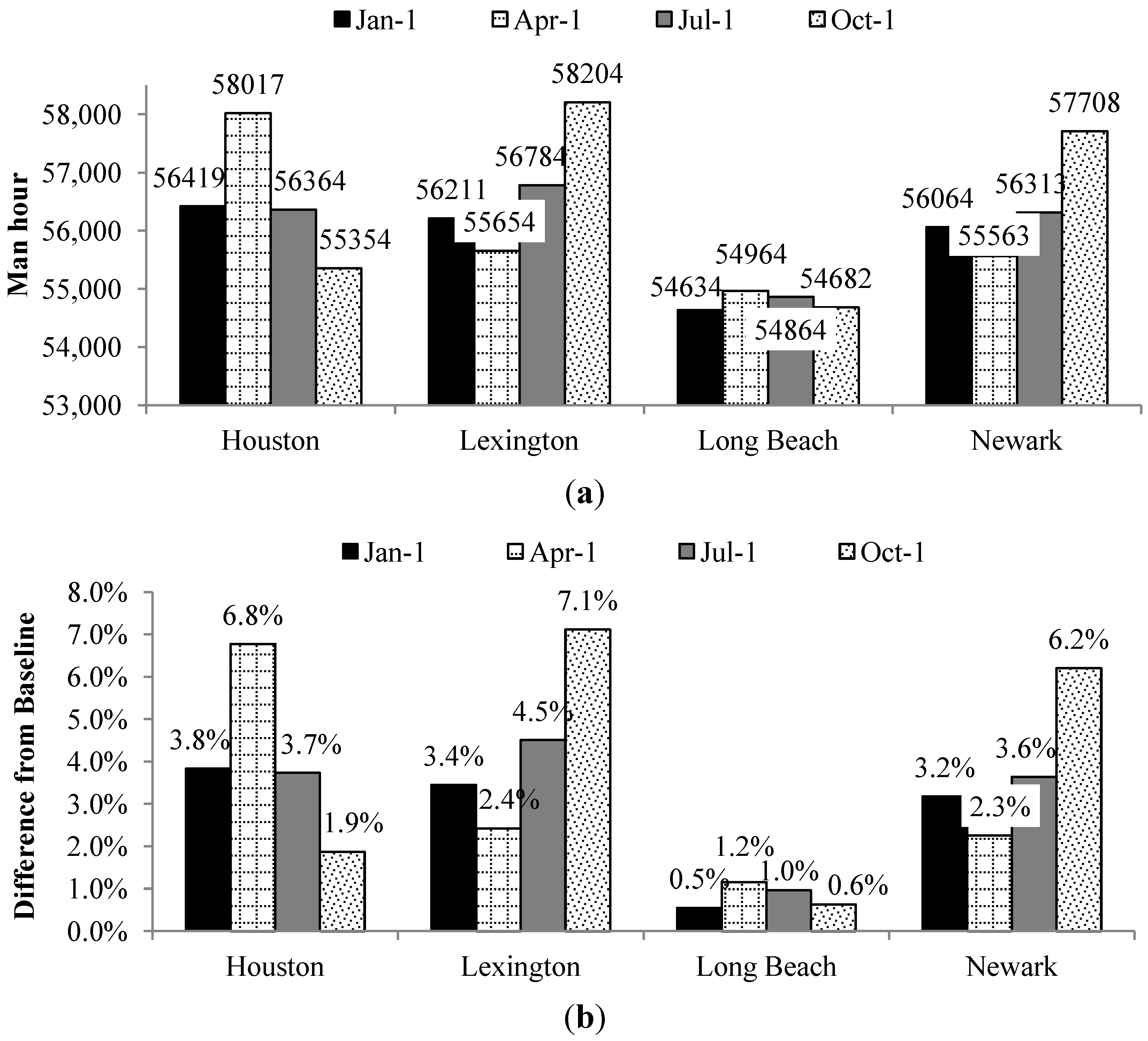
6.1. Descriptive Statistics

Table 5 shows the descriptive statistics for the generated simulation data on total man hours required to build the model project and the deviation from baseline (54,337 man hours) in percentage, considering the selected project locations and start dates. Since the baseline did not consider the temperature and humidity effect, the deviation from the baseline can be interpreted as the effect of temperature and humidity on the model project. The sample size for each block is 196. On average, building the model project in Long Beach, California, has the least impact and requires 54,634 to 54,964 man hours and deviates from the baseline by only 0.5% to 1.2% with different project start dates. Lexington, KY and Newark, NJ share a similar climate pattern and have a similar magnitude of temperature and humidity impact.

Table 5. Mean of the Total Man hours and Project Duration Required with Respect to Each Project Location and Start Date.

Location		Man hours
		1 January	1 April	1 July	1 October
Houston	Mean	56,419	58,017	56,364	55,354
	∆ a	3.8%	6.8%	3.7%	1.9%
Lexington	Mean	56,211	55,654	56,784	58,204
	∆	3.4%	2.4%	4.5%	7.1%
Long Beach	Mean	54,634	54,964	54,864	54,682
	∆	0.5%	1.2%	1.0%	0.6%
Newark	Mean	56,064	55,563	56,313	57,708
	∆	3.2%	2.3%	3.6%	6.2%

Note: The Sample size for each block is 196. ^a Mean deviation from baseline in percentage.

Table 5. Mean of the Total Man hours and Project Duration Required with Respect to Each Project Location and Start Date.

Location		Man hours
		1 January	1 April	1 July	1 October
Houston	Mean	56,419	58,017	56,364	55,354
	∆ a	3.8%	6.8%	3.7%	1.9%
Lexington	Mean	56,211	55,654	56,784	58,204
	∆	3.4%	2.4%	4.5%	7.1%
Long Beach	Mean	54,634	54,964	54,864	54,682
	∆	0.5%	1.2%	1.0%	0.6%
Newark	Mean	56,064	55,563	56,313	57,708
	∆	3.2%	2.3%	3.6%	6.2%

Note: The Sample size for each block is 196. ^a Mean deviation from baseline in percentage.

6.2. Summary Results of Two-Way ANOVA

Table 6 shows the summary of two-way ANOVA of the total man hours. The results show that independent variables (Location and Start Date) and their interaction (Location × Start Date) have a statistically significant effect on the man hours required to build the model project, and the results are significant at 99% confidence level.

Table 6. Summary of Parametric Two-Way ANOVA of Total Man hours.

Source	Man Hours
	Sum of Square	d.f.	Mean Square	F	Sig.
Location	475,714,820.3	3	158,571,606.8	746.7	0.000
Start Date	44,225,292.2	3	14,741,764.1	69.4	0.000
Location × Start Date	442,459,960.7	9	49,162,217.9	231.5	0.000
Error	165,431,294.1	779	212,363.7	–	–
Total	1,126,200,776.6	794	–	–	–

Table 6. Summary of Parametric Two-Way ANOVA of Total Man hours.

Source	Man Hours
	Sum of Square	d.f.	Mean Square	F	Sig.
Location	475,714,820.3	3	158,571,606.8	746.7	0.000
Start Date	44,225,292.2	3	14,741,764.1	69.4	0.000
Location × Start Date	442,459,960.7	9	49,162,217.9	231.5	0.000
Error	165,431,294.1	779	212,363.7	–	–
Total	1,126,200,776.6	794	–	–	–

Figure 6. Bar Chart for Mean of Man Hours Required and Difference from Baseline in Percentage by Project Location across Four Project Start Dates.

Figure 6. Bar Chart for Mean of Man Hours Required and Difference from Baseline in Percentage by Project Location across Four Project Start Dates.

The bar chart in Figure 6 describes the mean of man hours required to build the model project and difference from baseline man hours in percentages by project location across four project start dates. Among the selected cities, the model project undertaken in Long Beach would experience the least negative impact on productivity as a result of temperature and humidity, ranging from 0.5% to 1.2%. This result is expected as Long Beach, CA has a consistent and mild climate with little variation in temperature. However, among the rest of the selected cities, project start date can play a significant effect; in the worst cases, the model project could suffer 6.8%, 7.1%, and 6.2% man-hour increases if the project starts 1 April in Houston, 1 October in Lexington, and 1 October in Newark, respectively. The differences in man-hours can be explained by the distinct climate among the selected cities. Houston has hot and humid summers, and construction peak falls into the window of summer can dramatically impact productivity negatively. Lexington, KY and Newark, NJ’s cold winters have a substantial impact on labor productivity, hence the project performance.

6.3. Multiple Pairwise Comparisons

To further investigate where the statistically significant differences lie within the groups, multiple pairwise comparisons were used to detect all possible statistically significant differences among all of the combinations of pairs. For this study, multiple pairwise comparisons were carried out using Tukey’s honest significant difference (HSD) test. Two major categories of tests were performed. One compares the difference in man hours between different project start date groups for each selected city. The other compares the difference in man hours between different project location groups for each selected project start date.

Table 7 shows the results of the multiple pairwise comparisons. For most of the cases, statistically significant differences were observed. For Houston, Lexington, and Newark, the differences of man hours required between different project start dates can even reach as many as over 2000 man hours, which represents a significant amount of labor costs. In regards to Long Beach, even though four out of the six comparisons were statistically significantly different, the magnitude of difference was not considerable, ranging from 48.1 to 329.9 man hours.

Table 7. Multiple Pairwise Comparisons of Man Hours Required between Various Project Start Dates by Location.

Location	Start Date	Man Hour [Mean Diff. (p-value)]
		1 April	1 July	1 October
Houston	1 January	−1597.9 (0.000)	55.3 (0.941) *	1065.4 (0.000)
	1 April	–	1653.2 (0.000)	2633.3 (0.000)
	1 July	–	–	1010.1 (0.000)
Lexington	1 January	557.2 (0.000)	−573.5 (0.000)	−1993.1 (0.000)
	1 April	–	−1130.7 (0.000)	−2550.3 (0.000)
	1 July	–	–	−1419.7 (0.000)
Long Beach	1 January	−329.9 (0.000)	−230.2 (0.000)	−48.1 (0.626) *
	1 April	–	99.6 (0.062) *	281.8 (0.000)
	1 July	–	–	182.1 (0.000)
Newark	1 January	500.8 (0.000)	−249.7 (0.034)	−1644.6 (0.000)
	1 April	–	−750.5 (0.000)	−2145.4 (0.000)
	1 July	–	–	−1394.9 (0.000)

Note: The difference was derived from the subtraction the mean man hours corresponding to row headings by mean man hours corresponding to column headings. * denotes the difference is not statistically significant at 95% confidence level.

Table 7. Multiple Pairwise Comparisons of Man Hours Required between Various Project Start Dates by Location.

Location	Start Date	Man Hour [Mean Diff. (p-value)]
		1 April	1 July	1 October
Houston	1 January	−1597.9 (0.000)	55.3 (0.941) *	1065.4 (0.000)
	1 April	–	1653.2 (0.000)	2633.3 (0.000)
	1 July	–	–	1010.1 (0.000)
Lexington	1 January	557.2 (0.000)	−573.5 (0.000)	−1993.1 (0.000)
	1 April	–	−1130.7 (0.000)	−2550.3 (0.000)
	1 July	–	–	−1419.7 (0.000)
Long Beach	1 January	−329.9 (0.000)	−230.2 (0.000)	−48.1 (0.626) *
	1 April	–	99.6 (0.062) *	281.8 (0.000)
	1 July	–	–	182.1 (0.000)
Newark	1 January	500.8 (0.000)	−249.7 (0.034)	−1644.6 (0.000)
	1 April	–	−750.5 (0.000)	−2145.4 (0.000)
	1 July	–	–	−1394.9 (0.000)

Note: The difference was derived from the subtraction the mean man hours corresponding to row headings by mean man hours corresponding to column headings. * denotes the difference is not statistically significant at 95% confidence level.

Similarly, Table 8 shows the results of the multiple pairwise comparisons of man hours required between different project locations given the same specific project start date. Situating the model project to start on the first day of each quarter, the difference in required man hours among the cities shows a broad range, from 50.9 to 3521.9 man hours.

Table 8. Multiple Pairwise Comparisons of Man Hours Required between Various Project Locations by Start Date.

Start Date	Location	Man hour [Mean Diff. (p-value)]
		Lexington	Long Beach	Newark
1 January	Houston	208.5 (0.020)	1785.4 (0.000)	355.9 (0.000)
	Lexington	–	1576.9 (0.000)	147.4 (0.167) *
	Long Beach	–	–	−1429.5 (0.000)
1 April	Houston	2363.6 (0.000)	3053.4 (0.000)	2454.6 (0.000)
	Lexington	–	689.8 (0.000)	91.0 (0.581) *
	Long Beach	–	–	−598.8 (0.000)
1 July	Houston	−420.2 (0.000)	1499.9 (0.000)	50.9 (0.933) *
	Lexington	–	1920.1 (0.000)	471.1 (0.000)
	Long Beach	–	–	−1449.0 (0.000)
1 October	Houston	−2850.0 (0.000)	671.9 (0.000)	−2354.1 (0.000)
	Lexington	–	3521.9 (0.000)	495.9 (0.001)
	Long Beach	–	–	−3026.1 (0.000)

Note: The difference was derived from the subtraction the mean man hours corresponding to row headings by mean man hours corresponding to column headings. * denotes the difference is not statistically significant at 95% confidence level.

Table 8. Multiple Pairwise Comparisons of Man Hours Required between Various Project Locations by Start Date.

Start Date	Location	Man hour [Mean Diff. (p-value)]
		Lexington	Long Beach	Newark
1 January	Houston	208.5 (0.020)	1785.4 (0.000)	355.9 (0.000)
	Lexington	–	1576.9 (0.000)	147.4 (0.167) *
	Long Beach	–	–	−1429.5 (0.000)
1 April	Houston	2363.6 (0.000)	3053.4 (0.000)	2454.6 (0.000)
	Lexington	–	689.8 (0.000)	91.0 (0.581) *
	Long Beach	–	–	−598.8 (0.000)
1 July	Houston	−420.2 (0.000)	1499.9 (0.000)	50.9 (0.933) *
	Lexington	–	1920.1 (0.000)	471.1 (0.000)
	Long Beach	–	–	−1449.0 (0.000)
1 October	Houston	−2850.0 (0.000)	671.9 (0.000)	−2354.1 (0.000)
	Lexington	–	3521.9 (0.000)	495.9 (0.001)
	Long Beach	–	–	−3026.1 (0.000)

Note: The difference was derived from the subtraction the mean man hours corresponding to row headings by mean man hours corresponding to column headings. * denotes the difference is not statistically significant at 95% confidence level.

6.4. Implications of the Statistical Analyses

The results of the two-way ANOVA show that the main effect, project start date and location, can significantly impact the man hours required to build the model project, and that project start date and location interactively influence the total man hours. This finding is very intuitive since geographic location and season jointly contribute to the different weather patterns, consequently affecting craft workers’ productivity.

The multiple pairwise comparisons have a number of merits for various parties involved in a project depending on the perspective of each party. Fixing the project location and comparing the man hours required between different project start dates enable contractors to understand the magnitude of man hour differences attributed to the temperature and humidity’s impact on labor productivity due to varied project start dates, so that when they bid their projects they can take the difference into consideration, which renders more accurate estimates. Take this particular model project examined in this study as an example. On average, when the project located in Lexington starts its execution on 1 October, the total man hours required to build the project increase by 2550 h (4.6%) compared to the man hours required when the project starts on 1 April. Four-point-six percent is a very substantial number to the construction industry in that the average net profit of the construction industry is 6.33% [38]. With a lower profit margin, an accurate cost estimate is very essential for a contractor’s success [39]. From the point of view of owners, if the schedule is not the primary driver over costs, owners can plan to start a project at an optimal timing which could render the lowest project costs. Supposing all other evaluation criteria are the same; owners also can use the statistical results to select the best location from a list of potential project locations that require the lowest construction costs.

The statistical analysis results can also provide a unique dimension in regard to project portfolio management (PPM) for business owners who conduct business across the country. The objectives of PPM are to maximize the contributions of a collection of projects to the overall financial and operational goals of an organization with various imposed constraints [40]. Major retailers, such as Walmart, Target, Lowes, and Home Depot, often have buildings built at different locations with similar footprints and designs. It is very likely that owners could have proposed a few projects that are going to be built at a collection of selected project locations. By implementing the framework and performing statistical analyses on generated simulation results, decision makers can acquire more confident information to optimize the construction costs of the project portfolio by scheduling each project at a specific location with a better project start date, which would minimize the negative impact due to unfavorable temperature and humidity conditions. The authors readily acknowledge that the project costs are just one of the factors being considered during the process of PPM; however, the concept proposed in this study extends an extra dimension to the existing decision making criteria.

Besides the accuracy of man hour estimates provided by the framework that integrates BIM with productivity and productivity factors, another advantage of using BIM to perform the described study is the 4D schedule analysis. Side-by-side comparison of multiple 4D schedule animations allows construction practitioners to visualize the productivity changes under different project execution scenarios. Figure 7 demonstrates an example of the schedule performance comparison using a 4D schedule analysis when the model project is built with two different start dates, 2 April 2007 and 1 October 2007 in Lexington, KY. The second and third columns represent the progress statuses at five different time points (105, 150, 168, 196, and 245 calendar days elapsed) after the project starts on 2 April 2007 and 1 October 2007. The differences are highlighted with red circles. As shown in Figure 7, the project that starts on 2 April 2007 progresses faster than the project that starts on 1 October 2007. The 4D schedule analysis renders a straightforward presentation with minimal stress on human beings’ cognitive loading.

7. Conclusions and Limitations

This research provides a framework of integrating BIM and CPM schedules to simulate the temperature and humidity impact on productivity at a project level. The research effort took a model project as a test model and selected four project locations in the U.S. and their last 50 years of historical weather data to demonstrate the applicability of the framework. The demonstration of the statistical analyses of the simulated results shows how the simulation results can be exploited to generate knowledge for decision making. Since this study took a specific model project and four project locations, the results of the study cannot be directly applied to a different project. Therefore, the external validity of the statistics might be limited. However, the external validity of the developed framework is still preserved. The readers should direct their attention to the framework, because the concept can be generalized to any project. In addition, the BIM-based framework can have a broader use, such as simulating overtime and craft density’s effect on labor productivity at the project level.

Figure 7. Comparison of Schedule Performance between Project Start Date 4/2 and 10 January 2007 in Lexington, KY.

Figure 7. Comparison of Schedule Performance between Project Start Date 4/2 and 10 January 2007 in Lexington, KY.

Note: Gray color represents the work at the beginning stage; color represents the work completed.

Based on the statistical analysis of the simulation results, the generalized findings that are drawn are as follows:

(1)

Temperature and humidity difference due to project geographical location can significantly impact the man hours required to build a project;

(2)

Temperature and humidity difference due to seasonal effects can also significantly impact the man hours required to build a project; and

(3)

Project location and start date have an interaction in affecting the man hours required to build a project.

This research will contribute to the overall body of knowledge in the construction industry in several unique ways:

(1)

Project estimators can use this framework to simulate the temperature and humidity effects on their projects and better estimate their effects at the project level, as such to improve the certainty level of the project estimation.

(2)

For project decision makers, this research provides a unique venue of helping decision makers to evaluate how project start dates could influence labor productivity, thus influence project durations and costs.

(3)

This research also adds a dimension to evaluation criteria that a company can use for site selection when considering expanding their business to new geographic locations.

(4)

Business owners who standardize their project designs and operate the business across the country can use this framework to optimize project portfolio construction costs.

The limitations of the research are:

(1)

This research is built on an existing productivity model that describes the relationship between the productivity factor and temperature and humidity. The validity of this research relies on the validity of the chosen model.

(2)

Only the steel trade is examined for this project because the BIM application used for this research targets piping and steel trades.

(3)

This research used the same model project to test the temperature and humidity effect with respect to project locations. However, project locations might have an influence on materials size and types due to varied design load and code requirements.

(4)

This research did not take precipitation (rainfalls or snowfalls) into consideration. To use this framework to perform a simulation in those regions with excessive seasonal perception, the user needs to customize the workable day table to exclude some rainy days from the working days.

(5)

This research used historical weather data to perform the simulation. In order to harness this model as a predictive model, weather data projections obtained from a robust weather generator are needed.

References

1. Benjamin, N.B.H.; Greenwald, T.W. Simulating effects of weather on construction. J. Constr. Div. 1973, 99, 175–190. [Google Scholar]
2. Occupational Safety and Health Administration (OSHA). Tips to Protect Workers in Cold Environments. Available online: http://www.osha.gov/as/opa/cold_weather_prep.html (accessed on 23 February 2013).
3. Hancher, D.E.; Abd-Elkhalek, H.A. The effect of hot weather on construction labor productivity and costs. Cost Eng. 1998, 40, 32–36. [Google Scholar]
4. Koehn, E.; Brown, G. Climatic effects on construction. J. Constr. Eng. Manag. 1985, 111, 129–137. [Google Scholar] [CrossRef]
5. NECA. The Effect of Temperature Productivity; National Electrical Contractor Association, Inc.: Washington, DC, USA, 1974. [Google Scholar]
6. Grimm, C.T.; Wagner, N.K. Weather effects on mason productivity. J. Constr. Div. 1974, 100, 319–335. [Google Scholar]
7. Thomas, H.R.; Yiakoumis, I. Factor model of construction productivity. J. Constr. Eng. Manag. 1987, 113, 623–639. [Google Scholar] [CrossRef]
8. Carr, R.I. Simulation of construction project duration. J. Constr. Div. 1979, 105, 117–128. [Google Scholar]
9. Smith, G.R.; Hancher, D.E. Estimating precipitation impacts for scheduling. J. Constr. Eng. Manag. 1989, 115, 552–566. [Google Scholar] [CrossRef]
10. Shahin, A.; AbouRizk, S.M.; Mohamed, Y. Modeling weather-sensitive construction activity using simulation. J. Constr. Eng. Manag. 2011, 137, 238–246. [Google Scholar] [CrossRef]
11. Apipattanavis, S.; Sabol, K.; Molenaar, K.R.; Rajagopalan, B.; Xi, Y.; Blackard, B.; Patil, S. Integrated framework for quantifying and predicting weather-related highway construction delays. J. Constr. Eng. Manag. 2010, 136, 1160–1168. [Google Scholar] [CrossRef]
12. Construction Management Association of America (CMAA). Available online: http://cmaanet.org/ (accessed on 22 February 2014).
13. Construction, McGraw-Hill. The Business Value of BIM in North America: Multi-Year Trend Analysis and User Ratings (2007–2012); McGraw-Hill Construction: Bedford, MA, USA, 2012; pp. 9–16. [Google Scholar]
14. Hagan, S.; Ho, P.; Matta, H. BIM: The GSA story. J. Build. Inf. Model. 2009, 2009, 27–29. [Google Scholar]
15. Mayo, G.; Giel, B.; Issa, R. BIM use and requirements among building owners. In Proceedings of the International Conference on Computing in Civil Engineering, Clearwater Beach, FL, USA, 17–20 June 2012.
16. Krygiel, E.; Nies, B. Green BIM: Successful Sustainable Design with Building Information Modeling; Sybex: Indianapolis, IN, USA, 2008. [Google Scholar]
17. Azhar, S.; Carlton, W.A.; Olsen, D.; Ahmad, I. Building information modeling for sustainable design and LEED® rating analysis. Autom. Constr. 2011, 20, 217–224. [Google Scholar] [CrossRef]
18. Stumpf, A.; Kim, H.; Jenicek, E. Early Design Energy Analysis Using Bims (Building Information Models). In Proceedings of the Construction Research Congress, Seattle, WA, USA, 5–7 April 2009.
19. Cho, Y.K.; Alaskar, S.; Bode, T.A. BIM-integrated sustainable material and renewable energy simulation. In Proceedings of the Construction Research Congress 2010: Innovation for Reshaping Construction Practice, Banff, AB, Canada, 8–10 May 2010.
20. Eastman, C.M.; Teicholz, P.; Sacks, R.; Liston, K. BIM Handbook: A Guide to Building Information Modeling for Owners, Managers, Architects, Engineers, Contractors, and Fabricators, 2nd ed.; John Wiley & Sons, Inc.: Hoboken, NJ, USA, 2011; pp. 221–222. [Google Scholar]
21. Lu, N.; Korman, T. Implementation of Building Information Modeling (BIM) in modular construction: Benefits and challenges. In Proceedings of the Construction Research Congress 2011, Banff, AB, Canada, 8–10 May 2010.
22. Leite, F.; Akinci, B.; Garrett, J. Identification of data items needed for automatic clash detection in MEP design coordination. In Proceedings of the Construction Research Congress, Seattle, WA, USA, 5–7 April 2009.
23. Tan, X.; Hammad, A.; Fazio, P. Automated code compliance checking for building envelope design. J. Comput. Civ. Eng. 2010, 24, 203–211. [Google Scholar] [CrossRef]
24. Nawari, N.O. Automating codes conformance. J. Archit. Eng. 2012, 18, 315–323. [Google Scholar] [CrossRef]
25. Santos, I.; Farinha, F. Code checking automation in building design: New trends for cognition. Comput. Civ. Eng. 2005, 179, 1–8. [Google Scholar]
26. Ibrahim, M.M.; Krawczyk, R.J. A web-based approach to transferring architectural information to the construction site based. In Proceedings of the CAADRIA 2004 Conference: Culture, Technology and Architecture, Seoul, Korea, 28–30 April 2004.
27. Sabol, L. Building Information Modeling & Facility Management; IFMA World Workplace: Dallas, TX, USA, 2008. [Google Scholar]
28. Chau, K.W.; Anson, M.; Zhang, J.P. Implementation of visualization as planning and scheduling tool in construction. Build. Environ. 2003, 38, 713–719. [Google Scholar] [CrossRef]
29. Moon, H.; Dawood, N.; Kang, L. Development of workspace conflict visualization system using 4D object of work schedule. Adv. Eng. Inform. 2014, 28, 50–65. [Google Scholar] [CrossRef]
30. Zhang, S.; Teizer, J.; Lee, J.-K.; Eastman, C.M.; Venugopal, M. Building information modeling (BIM) and safety: Automatic safety checking of construction models and schedules. Autom. Constr. 2013, 29, 183–195. [Google Scholar] [CrossRef]
31. Zhou, Y.; Ding, L.Y.; Chen, L.J. Application of 4D visualization technology for safety management in metro construction. Autom. Constr. 2013, 34, 25–36. [Google Scholar] [CrossRef]
32. Chen, S.-M.; Griffis, F.H.; Chen, P.-H.; Chang, L.-M. A framework for an automated and integrated project scheduling and management system. Autom. Constr. 2013, 35, 89–110. [Google Scholar] [CrossRef]
33. National Institute of Standards of Technology (NIST). CIS/2 and IFC—Product Data Standards for Structural Steel. Available online: http://cic.nist.gov/vrml/cis2.html (accessed on 1 March 2014).
34. Richardson Construction Estimating Standards. Available online: http://www.costdataonline.com/Richardson.htm (accessed on 2 March 2014).
35. Bunea, S.P. Means Structural Steel Estimating: Miscellaneous Iron, Ornamental Metals; Robert S Means Co.: Kingston, MA, USA, 1987. [Google Scholar]
36. Weather Underground. About Our Data. Available online: http://www.wunderground.com/about/data.asp (accessed on 3 March 2014).
37. Construction Industry Institute-RT272. Enhance Work Packaging: Design through Workface Execution; Construction Industry Institute: Austin, TX, USA, 2012. [Google Scholar]
38. BizStats BizMiner Industry Reports. Available online: http://bizstats.com/corporation-industry-financials/construction-23/show (accessed on 3 March 2014).
39. Waddle, T.W. Bid preparation for contractors (Avoiding Estimating Errors). In Proceedings of the 53rd AACE International Annual Meeting, Seattle, WA, USA, 5–7 April 2009.
40. Rajegopal, S.; Waller, J.; McGuin, P. Project Portfolio Management: Leading the Corporate Vision; Palgrave Macmillan: Basingstoke, UK, 2007; pp. 3–12. [Google Scholar]