Assessment of the Impact of Cool Roofs in Temperate Climates through a Comparative Experimental Campaign in Outdoor Test Cells

Abstract

Over the last few decades many bibliographical studies have been conducted on cool roofs, by analyzing both the energy performance during summer and winter seasons and their contribution in mitigating the urban heat island effect. This paper describes the experimentation carried out in three outdoor test cells to comparatively assess the behavior of a cool roof solution with respect to a ventilated-roof and a warm-roof. The monitored data have confirmed that in summer cool roofs are the best solution, with respect to traditional tile roofing, sensibly reducing surface temperatures as a function of the solar direct radiation level (15–25 °C for I > 600 W/m² and 5–15 °C for I < 300 W/m², independently of the season). Furthermore, cool roofs involve an energy saving related to summer cooling by about 20% as to a warm-roof and 15%–20% as to a vented-roof. During winter, cool roofs improve the heating energy performance of a vented-roof by about 12%, against a slightly increased consumption (<5%) if compared to a warm-roof. These data confirm that, in temperate climates, cool roofs are appropriate solutions to sensibly improve summer energy performances with a negligible negative impact during winter, and to positively contribute to the mitigation of the heat island effect.

1. Introduction

Over the last few decades many bibliographical studies have focused their attention on the investigation of cool roofs and cool materials for roofs, analyzing both their contribution in mitigating the urban heat island phenomenon and the effects on the energy performances of buildings during summer and winter seasons in different climate contexts.

The ‘Urban heat Island effect’ is a particular physical phenomenon leading to higher temperatures in urban areas than in the surrounding rural areas [1,2,3]. Higher urban temperatures have a negative impact on: cooling energy demand [4] and cooling peak energy demand [5]; the production of atmospheric ozone [6,7,8,9], one of the main components of urban smog; air pollution level [10], human health [11,12,13] and the perception of well-being [14].

This phenomenon is mainly due to anthropogenic causes [10], including increasing urbanisation often leading to: reduced albedo values of urban surfaces materials [9,15,16], very little green areas [8] and ‘wet’ surfaces [8,13] often caused by inadequate and uninformed urban planning policies that over the decades have led to a progressive deterioration of the situation.

The mitigation of the urban heat island (UHI) phenomenon can be mainly achieved by applying numerous and different measures aimed at:

• reducing surface temperatures, through the modification of the thermal and radiative characteristics of urban surfaces materials [17,18];
• lowering the anthropogenic impact [19], both directly, by reducing building heating/cooling energy consumptions [9,20], and indirectly, by reducing greenhouse gas emissions that can alter the atmospheric radiative forcing [16,21,22];
• modifying and increasing the vegetative cover of the metropolitan areas [8,23], for example implementing tree planting programs;
• enhancing urban ventilation [24].

Cool materials, and consequently cool roofs, can positively contribute to implement the measures illustrated above in the first two entries: cool roofs are in fact characterized by external surface materials conceived to reflect a large amount of incident solar radiation [25], sensibly reducing both the surface temperatures and the absorbed heat, and then the fraction of heat that is released in the urban environment in the following hours.

At the same time, a lower surface overheating means a significant reduction of heat entering buildings through opaque closures by conduction, with a reduction of summer cooling loads [26] corresponding to smaller releases of polluting greenhouse gases into the atmosphere [19].

Many of the bibliographical studies reviewed in literature concerning the UHI mitigation measures are about the simulation, through global climate models, of the effects caused by the modification of the urban surface albedo [20,21,22].

Many other authors have instead analysed and demonstrated the effectiveness and the benefits of adopting cool roofs to reduce the energy consumptions of buildings for summer cooling in different climates [9,20,23,26,27,28,29,30,31,32], considering buildings with different end uses [29,31,33,34].

Results and conclusions of all those studies have demonstrated that cool roofs are one of the most performing solutions in terms of benefits with respect to both the mitigation of the UHI phenomenon and the reduction of summer cooling loads.

The study of the behavior of cool roof during the winter appears, on contrary, more complex.

Some studies have focused their attention on the winter behavior of cool roofs in terms of expected heating penalty in temperate and cold climates. The supposed solar heat gain loss by reflection [21] could in fact lead to a significant additional expenditure related to the heating of each individual building, even taking into account some studies [32] which demonstrate that during the winter season the UHI effect may result in an average temperature higher in urban centers than in rural areas therefore partially mitigating its harshness. However, the conclusions reached by those studies are not as uniform and consistent.

Most of the researches have demonstrated that cool roofs involve an annual energy penalty due to their performance in winter [35], considering both analysis of the whole urbanized areas through global climate models [21,31], and specific climatic contexts [28,33,36,37,38]. In contrast, some other authors have demonstrated that winter heating penalties for cool roofs are negligible in cold climates–even without the effect of snow–[21,39], depending on: the ratio of cloudy to sunny days (which increases during winter), less total solar radiation available on the roofs, the effect of snow.

The main goal of the present study is the comparative assessment of a cool roof solution though a two-year experimentation carried out in three outdoor test cells, with respect to a vented-roof and a warm-roof. The climate context of the experimentation is the ‘E’ zone of the Italian National legislation in force [40], and ‘Cfa’ for the Koppen-Geiger climate classification [41].

The paper involves an on-site monitoring to describe the comparative behavior of the cool roof under study both in summer and in winter season, considering also the effect of the roof performance deterioration after one year. At the same time, it involves an annual study of the effect of the cool roof on the external surface temperatures with respect to a traditional tile roofing (Canadian style tiles) as a function of global solar radiation and external temperatures, one of the most well-known strategies to mitigate the temperature rise of urban areas (UHI phenomenon).

2. Method: The Experimental Campaign in Outdoor Test Cells

The main goal of the experimental campaign is to compare the energy performances of a cool roof with respect to two roof solutions very common in Italy, a warm-roof and a vented-roof, in both passive and active conditions, at the latitudes of northern Italy, on the basis of a seasonal balance.

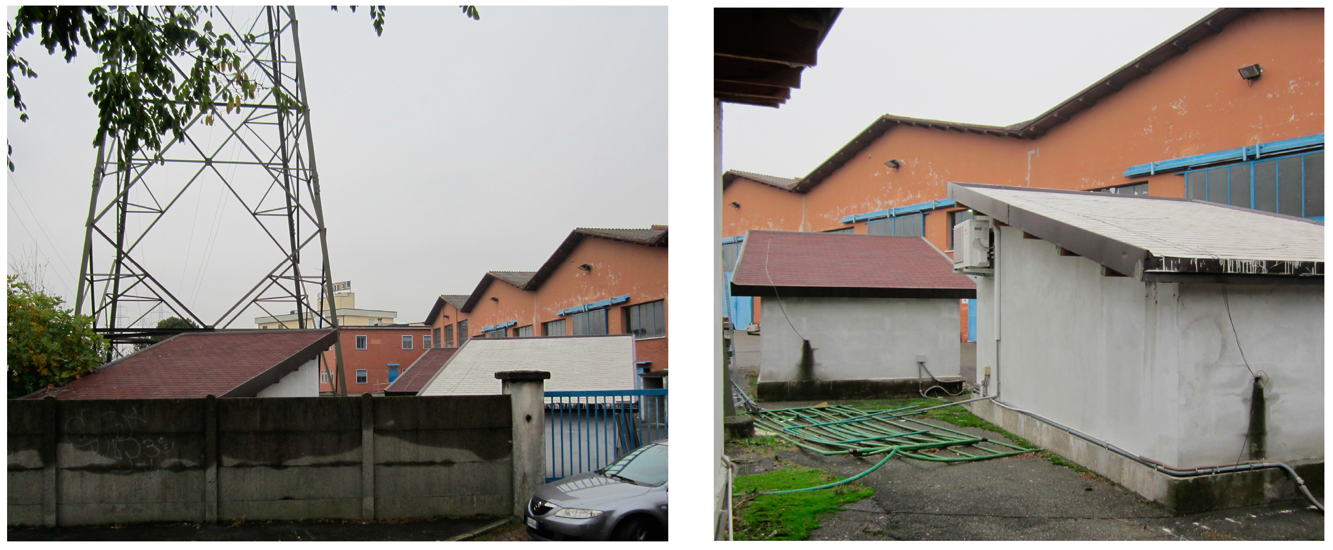
Three dedicated outdoor test cells were used during a period of eighteen months starting from July 2014. The cells are located at the headquarters of the Construction Technologies Institute of the National Research Council of Italy (ITC-CNR) in San Giuliano Milanese (Milano); they were built previously, calibrated and equipped with both an outdoor and indoor monitoring system used to analyze the main energy, environmental and comfort parameters related to the roof systems concerned, were used during a period of eighteen months starting from July 2014.

The experimental program is based on a multi-level approach:

• characterization of the roof system, through the performance evaluation of: indoor and outdoor surface temperatures, thermal transmittance over time, thermal wave attenuation and phase shift;
• characterization of the indoor environment, through the monitoring of the following indoor parameters: air temperature, radiant temperature, relative humidity, and the evaluation of the comfort indexes (PMV-Predicted Mean Vote- and PPD-Percentage of Persons Dissatisfied-);
• evaluation of energy consumption, through the accounting of consumption for the winter/summer air conditioning.

With regard to the cool roof characterization phase, some analyses related to the performance deterioration of the reflective capacity due to fouling and aging caused by natural and anthropogenic agents, were carried out through the analysis of monitored data and laboratory tests data relating to the summer periods of 2014 and 2015.

2.1. Description of the Experimental Set-Up

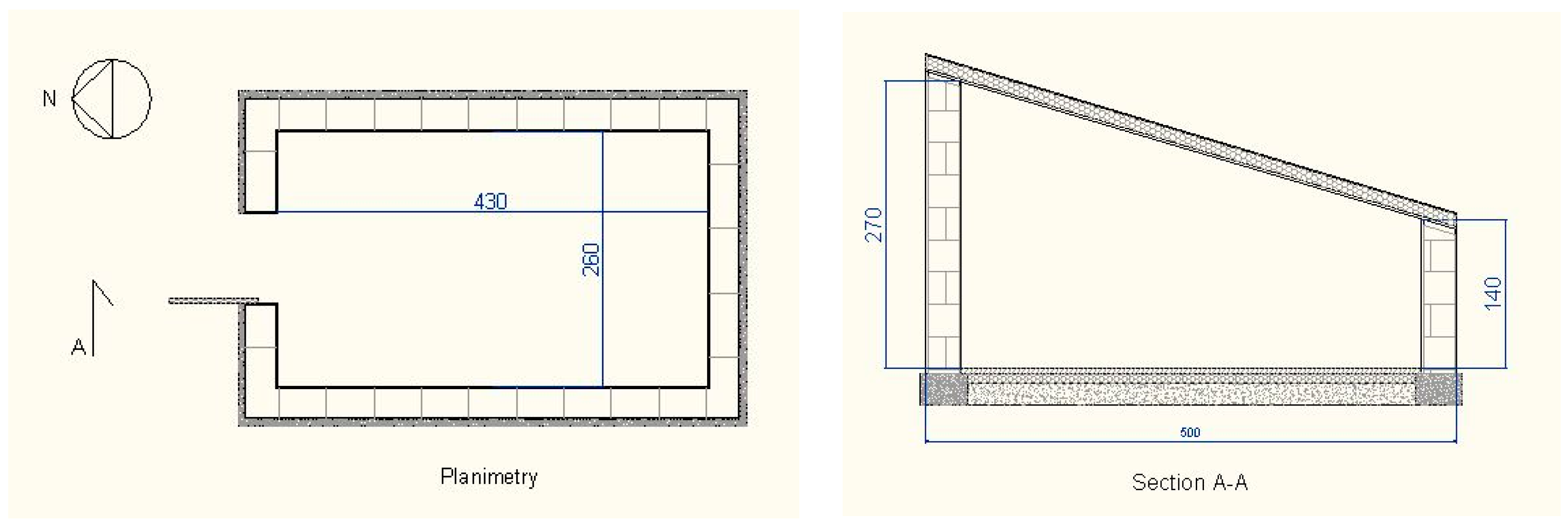
The three outdoor test cells, hereinafter referred to as C1, C2 and C3, were previously built with the same geometric, architectural and thermo-physical characteristics. Their indoor dimensions are 4.3 m × 2.6 m with a maximum and minimum height of 2.7 m and 1.4 m, respectively, corresponding to an inclination of a 30% pitch (Figure 1). The opaque vertical closures are built with 30 cm thick lightweight concrete blocks masonry with external insulation, while the lower horizontal partitions consist of a cast cement slab and sand with electro welded wire mesh and indoor insulation. The thermal transmittance of walls and floor comply with the minimum requirements provided for by the national legislation in force [18] relating to climate zone E, and they are 0.315 W/m²K and 0.326 W/m²K, respectively.

As regards the roof systems, three different experimental configurations were implemented: C1 (also referred to also as reference cell) warm-roof system; C2 (or cool roof) the same C1 warm-roof but equipped with an external cool finishing with high solar reflectance; C3 (or vented-roof) a vented solution.

Table 1. Roofing systems characteristics by UNI EN ISO 6946:2008 [42].

	Total Thickness (m)	Surface Mass (kg/m2)	Thermal Resistance (m2K/W)	Thermal Transmittance (W/m2K)	Thermal Periodic Transmittance (W/m2K)	Attenuation Factor	Thermal Lag (h)	Thermal Capacity 1 (Kcal/m2K)
C1	0.153	32.85	3.545	0.282	0.243	0.861	3.846	31.201
C2	0.153	32.85	3.545	0.282	0.243	0.861	3.846	31.201
C3	0.136	14.50	3.452	0.290	0.269	0.930	1.999	28.442

¹ The heat capacity of roofing systems, as well as their U-value, are key thermal parameters that define the main performances of the system under consideration [32]. As clearly shown by the data of Table 1 such values ensure greater comparability of results with respect to the characterizing parameters and consumption related to the three roofing solutions considered.

shows the main characteristics of the three roofing systems concerned, calculated in accordance with the relevant international standard [42].

The cells were equipped with a split system for summer cooling placed on the north wall, a floor fan heater for heating in winter and a tower fan. The tower fan worked in both active and passive mode, to prevent vertical temperature stratifications. All plant equipment has been connected to an electrical outlet with energy meter.

The cells are also equipped with a thermostat aimed at maintaining a constant indoor air temperature. The thermostatic temperature was set at 20 °C for both winter and summer seasons.

Usually, according to the EN 15251:2008 [43], the thermostatic temperature should be set to 20 °C in winter and to 26 °C in summer to better reproduce the operative conditions of conditioning plants. However, in this specific case, the choice to set the thermostatic temperature to 20 °C both for summer and winter season was dictated by both the small size of the indoor environment of the cells and the high level of insulation of the closures, in order to ensure a heating/cooling consumption suitable for energy analyses. Some previous experimental tests with a thermostatic temperature set at 26 °C, in fact, have shown how, during summer season, the conditioning energy consumption would have been too small to be compared between the three test cells.

This initial hypothesis is also supported by the following consideration: the outdoor test cells are not conceived to reproduce real operative conditions. The cells are in fact too small for this goal; so, the energy consumptions both for heating and cooling are not considered in absolute terms. The cells are conceived to compare the energy behavior of three different roof systems and to quantify in percentage energy consumptions on a seasonal basis, each test cell with respect to the other two.

The cells were equipped with the monitoring system too, for the acquisition of physical and environmental parameters useful to the characterization of the three coverage systems concerned and the cells energy performances.

2.2. Specifics of the Cool Roof System

The three test cells have two different roof external finishing systems (Figure 2): C1 and C3 dark red ‘Canadian’ style tiles; C2 the same tile kind but covered with a high solar reflectance white paint.

In cooperation with ENEA (Italian National Agency for New technologies, Energy and Sustainable Economic Development), some laboratory tests were carried out to evaluate the spectral reflectance of two samples taken from C1 and C2 roofing systems, respectively, coinciding with the start of the experimental campaign. The samples were analysed with a double beam spectrophotometer from which is derived the trend of the reflectance value as a function of the incident beam wavelength between 300 and 2500 nanometres [44]. The integration according to ISO 9050:2003 [45] was performed based on the spectrophotometer data; such integration provides for the calculation of a weighted average of the reflectance values in the considered band (300 nm–2500 nm) following the energy distribution of the solar spectrum, assigning greater weight to the visible and the infrared band up to about 1200 nm and, at the same time, a very low weight to the UV band.

Table 2. Calculation of the integrated reflectance [45]—expressed in percentages—and the corresponding absorption coefficient.

	Tile with High Solar Reflectance White Paint	Canadian Style Tile
Rvis	82.6	6.50
R	71.3	8.50
a	0.29	0.92
e	>0.90	>0.80

Notes: Solar Reflectance, visible spectrum—Rvis; integrated solar Reflectance—R; absorption coefficient—a; emissivity—e.

summarizes the calculated solar reflectance (R) obtained through the weighted procedure laid down in the ISO standard [45], both as regards only the visible range (380–760 nm, Rvis), and the full spectrum (300–2500 nm, R).

The calculated value of the integrated reflectance on the full spectrum (R) of the two materials represents a very significant parameter because the absorption coefficient (a) of a material is calculated starting from the solar reflectance. The direct radiant energy incident on a surface, in fact, is composed of three components: a reflected (R), an absorbed (a) and a transmitted (t) one, mutually related by the following equation:

R + a + t = 1

(1)

For opaque bodies—as in the specific case the shell of cells C1, C2 and C3—‘t’ is assumed equal to 0; so, the absorption coefficient (a) is calculated as:

a = 1 − R

(2)

2.3. The Monitoring System

The monitoring system of the three outdoor test cells consists of a weather station and indoor and outdoor sensors.

2.3.1. The Weather Station

The monitoring of the outdoor climatic conditions is carried out using a weather station at ITC-CNR. The weather station is a system similar to the one located in the outdoor cells, and it consists of a TMF500 data logger (NESA srl, Vidor, Treviso, Italy) [46] and a set of sensors for the detection of the following physical and environmental parameters: air temperature; humidity; direct solar radiation; wind speed, direction and elevation; horizontal and diffuse global illuminance; atmospheric pressure; rainfall.

2.3.2. Indoor Sensors

The outdoor test cells are equipped with an environmental monitoring and data acquisition system focused on the determination of indoor environmental test conditions, the characterization of the roofing system, the analysis of surface temperatures, the assessment of indoor comfort conditions and the recording of air conditioning energy consumptions.

The system consists of three data loggers and the set of sensors connected to them for the acquisition of the indoor environmental variables. The data loggers are of the TMF500 type and are the core of the remote control system monitoring and data acquisition units: each of them is placed in one of the three cells and has been configured for the collection and submission of data via FTP to a dedicated server through a LAN.

The acquisition of the indoor data is based on a five-minute time step; the processing of the monitored data is based instead on hourly averages.

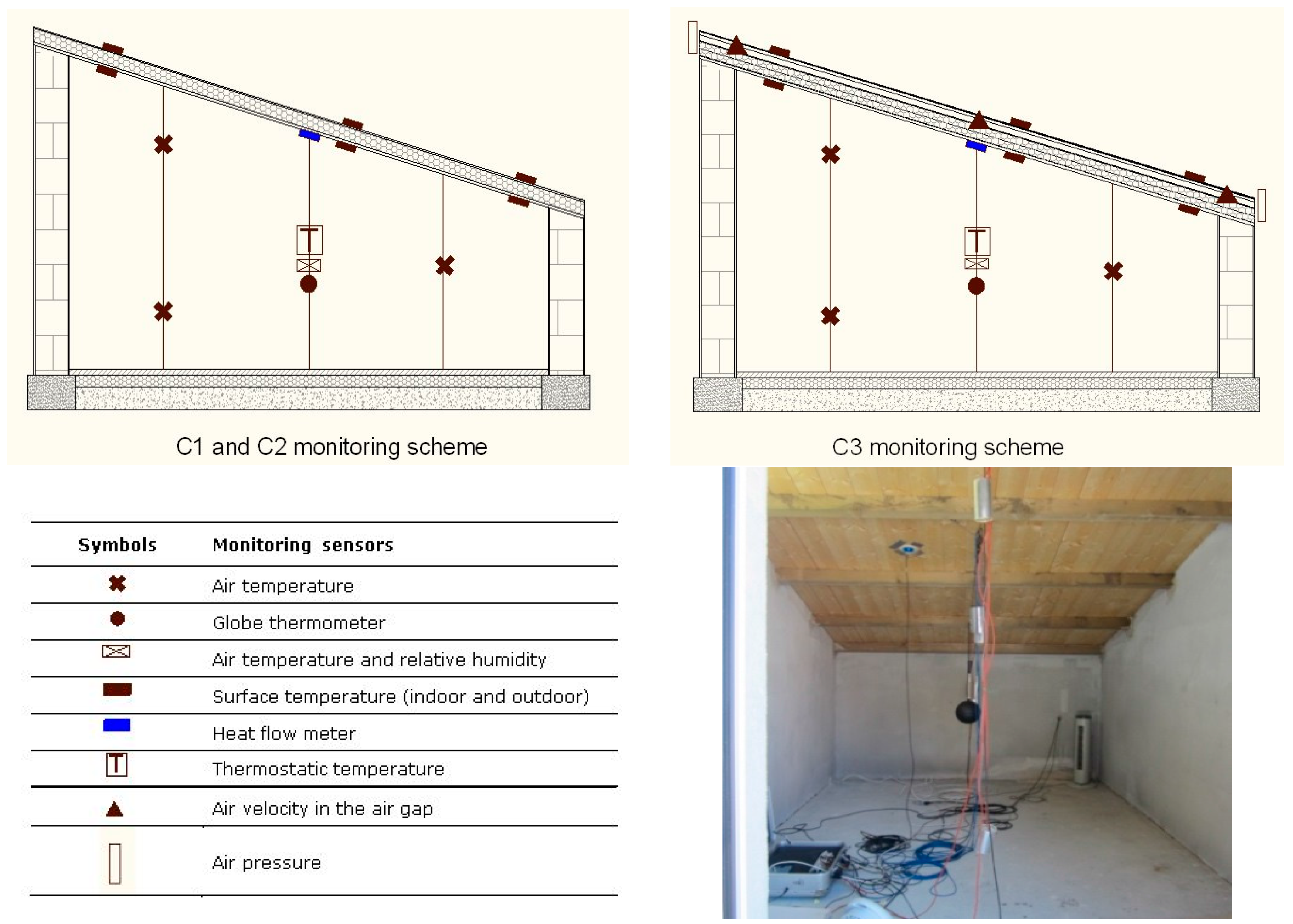
The pattern of the indoor spatial sensors configuration is the same in the three cells, and it involves the placement of: indoor air temperature sensors, globe thermometer, temperature and humidity sensors, surface temperature sensors and heat flow meter, as well as the temperature sensor connected with the thermoregulation system of the cell.

With regard to just the C3 roofing system (vented-roof), some parameters are also tracked at the entrance, at the middle and at the exit of the ventilation channel: air temperature and air velocity, pressure.

Figure 3 shows the indoor monitoring system scheme and an image of the inside of the cell, as shown in Figure 3.

2.3.3. Outdoor Sensors

When analyzing the performances of the three roofing systems, the external surface temperatures are monitored too, with three measuring points (Figure 3).

The acquisition and the processing of the outdoor data is based on the same time scale of the indoor data.

3. Results and Discussion

3.1. Charactersation of the Cool Roof System

The cool roof system was characterized following a four-stage procedure: the analysis of the surface temperatures (Tsup); the study of the thermal transmittance (U) trend and of the thermal attenuation and phase shift phenomena; and the in situ and laboratory test on the performance detriment level after one year of exposure to environmental and anthropogenic agents.

The performance detriment of the cool roof is an important topic because the loss of the reflective capacity of the cool coating can appreciably influence both the external surface temperatures of the roof, with a significant increase, and the energy consumption on a seasonal basis (a potential increase of summer cooling loads).

3.1.1. The Surface Temperatures Analysis

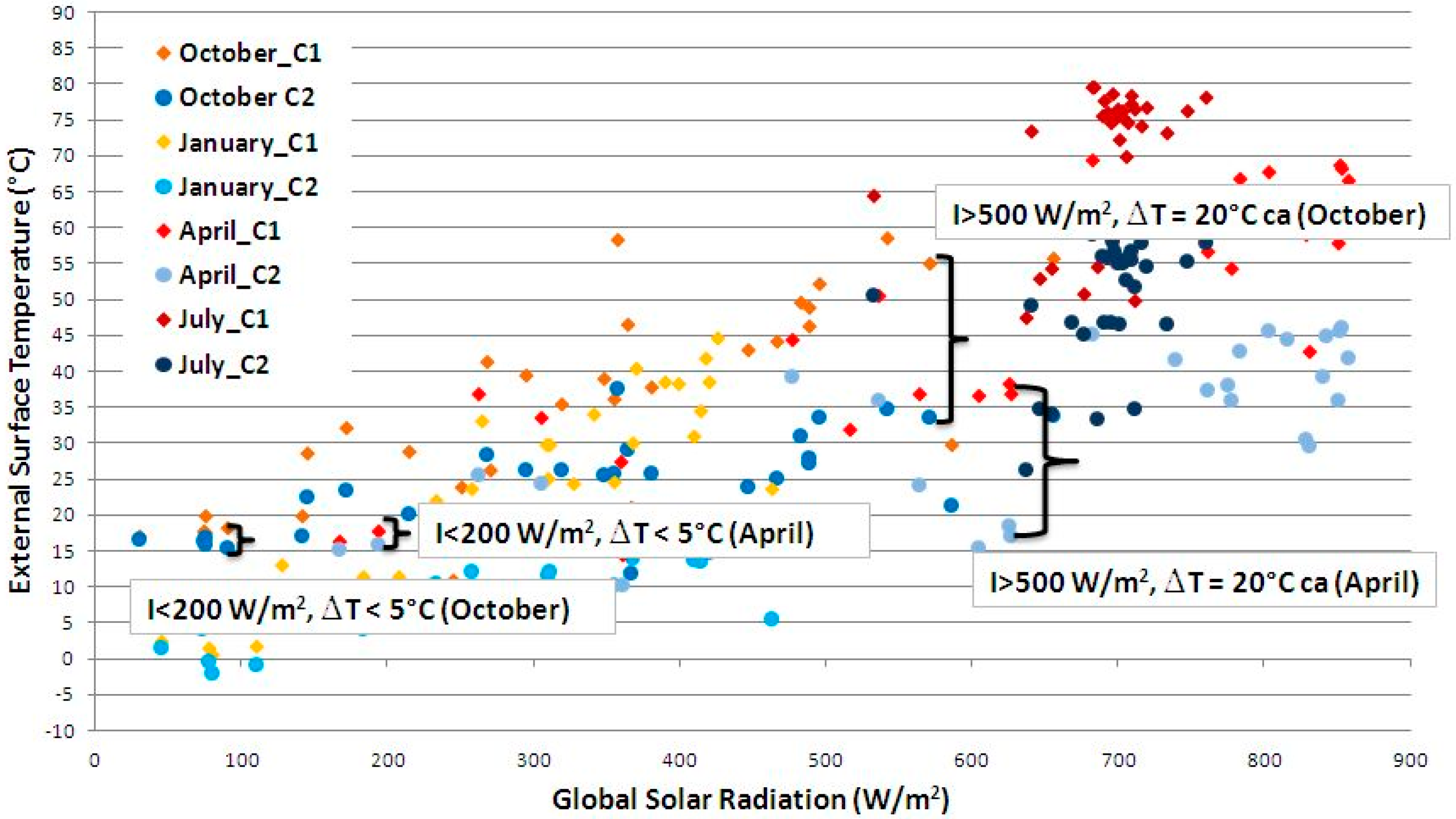
The graphs related with the external surface temperatures (Tsup) trends on a seasonal basis, highlighted how the thermal gradients between a cool roof and a roof finished with dark-colored tiles, depend on the global solar radiation. The external surface temperatures (Tsup) of an object exposed to the external environment is a function of both solar radiation level and external temperature; but, the analysis on an annual basis of the monitored data has allowed to verify how the external surface temperature gradients between C2 and C1 (C1 and C3 have the same surface temperature, due to the same finishing with dark-colored tiles) are almost constant on an annual basis in the set range of the incident solar radiation (

Table 3. External surface temperatures and thermal gradients as a function of the solar radiation level.

Global Solar Radiation	Clear Sky	Light Fog	Cloudy	Yellow Disc	White Disc	Perceptible Sun	Thick Fog
(W/m2)	1000–600	600–500	500–400	400–300	300–200	200–100	100–50
Summer 1
T1,3	58–75 °C	55 °C	45 °C	30 °C	25 °C	25 °C
T2	38–60 °C	35 °C	25 °C	25 °C	20 °C	20 °C	–
DT	15–20 °C	20 °C	20 °C	5 °C	5 °C	5 °C
Autumn 1
T1,3	60–65 °C	50–55 °C	40–55 °C	30–45 °C	25–35 °C	14–28 °C	10–20 °C
T2	35–40 °C	30–35 °C	25–35 °C	15–30 °C	10–25 °C	8–22 °C	8–15 °C
DT	25 °C	20 °C	15–20 °C	15 °C	15–20 °C	6 °C	2–5 °C
Winter 1
T1,3	40–50 °C	38–45 °C	28–45 °C	25–40 °C	15–35 °C	8–12 °C	5–10 °C
T2	30–35 °C	20–25 °C	15–25 °C	10–25 °C	8–20 °C	5 °C	3–5 °C
DT	10–15 °C	18–20 °C	13–20 °C	15 °C	7–15 °C	3–7 °C	2–5 °C
Spring 1
T1,3	45–75 °C	40–60 °C	40 °C	25–35 °C	25–30 °C	18–20 °C
T2	30–55 °C	30–40 °C	25 °C	18–30 °C	20–25 °C	15 °C	–
DT	15–20 °C	10–20 °C	15 °C	7–15 °C	5 °C	3–5 °C

Notes: Surface temperatures, cells C1 and C3—T_1,3; surface temperatures cell C2—T₂; thermal gradient (T_1,3 − T₂)—DT. ¹ Monitoring periods: summer (from 01.08.2014 to 22.09.2014); autumn (from 23.09.2014 to 21.12.2014); winter (from 22.12.2014 to 20.03.2015), spring (from 21.03.2015 to 21.06.2015).

). In contrast, the peak temperature achieved is a function of both the intensity of the solar radiation and of the external temperature.

Table 3 shows the average values of the external surface temperatures (Tsup) and the thermal gradients on a seasonal basis as a function of the solar radiation level, together with an excerpt of the graphical analysis (Figure 4) of the monitored data related to four months: October 2014, January, April and July 2015.

The data analysis has led to the following concluding remarks: in the presence of high direct solar radiation level (>600 W/m²) the annual range of the surface temperature (Tsup) values of the external cells was 50–60 °C for C1, and 30–40 °C for C2, confirming a gradient of about 20 °C on an annual average and irrespective of the season; in the presence of reduced direct solar radiation (<300 W/m² the annual range of the surface temperatures (Tsup) values of the cells was 15–25 °C for C1, and 10–20 °C for C2, confirming the expectations connected with the use of high solar reflective paint (about 5 °C less than an annual average always regardless of the season).

The most interesting conclusion that emerges is that the thermal gradient between the surface temperatures (Tsup) of a dark colored roof with respect to a cool roof depends more on the solar irradiance level than on the external temperature. Therefore, if during the summer season the positive contribution in reducing thermal loads due to the reflection of the sun heat gains is confirmed, a possible negative impact on the winter heating loads is a function of latitude and meteorology, i.e., the number of clear and extremely sunny days during the winter season: paradoxically, at very cold latitudes, where winter sunny days have a lower relevance, the ratio of cloudy to sunny days increase and the impact of global solar radiation on the roof is smaller [39], the cool roof has potentially less impact than at temperate or warm latitudes characterized by quite mild and sunnier winters.

The analysis of the external surface temperatures (Tsup) as a function of the external temperature and the solar radiation, has omitted the wind contribution as it is regarded as negligible.

Table 4. Monitored wind speed average on a seasonal basis, measured and tabled considering the Beaufort Force classification.

Season	Wind Speed (m/s)	Beaufort Force	Descriptive Term	Percentage Rate
Summer	0.3–1.5	1	Light air	57
	1.6–3.4	2	Light breeze	43
	3.4–5.6	3	Gentle breeze	–
Autumn	0.3–1.5	1	Light air	60
	1.6–3.4	2	Light breeze	20
	3.4–5.6	3	Gentle breeze	20
Winter	0.3–1.5	1	Light air	25
	1.6–3.4	2	Light breeze	54
	3.4–5.6	3	Gentle breeze	21
Spring	0.3–1.5	1	Light air	61
	1.6–3.4	2	Light breeze	26
	3.4–5.6	3	Gentle breeze	4

shows the percentage rate of the monitored wind speed on a seasonal basis.

In most cases, wind speed is within the limits of class 2 and less than 3 m/s. Therefore the wind contribution can be considerable negligible.

3.1.2. Study of Thermal Transmittance and Phase Shift and Attenuation Phenomena

The thermal transmittance was calculated using two different methodological approaches: the UNI EN ISO 6946 [42] calculation method and the measuring method with heat flow meter [47].

Considering the measuring method with heat flow meter, the chosen calculation process is based on progressive averages.

Table 5. The calculated thermal transmittance under the stated international standards.

	C1	C2	C3
U UNI EN ISO 6946	0.28	0.28	0.29
U ISO 9869	0.24	0.30	0.34

summarizes the calculated values for the three outdoor test cells roofing systems under UNI EN ISO 6946 and ISO 9869 standards [47].

The considerable discrepancy between the obtained data is due to the nature of the two calculation methods considered: the standardized approach of UNI EN ISO 6946 provides a normalized calculation guidance starting from steady state boundary conditions and in the absence of solar radiation, so not taking into account the real outdoor climatic conditions and at the same time introducing important simplifications: the action of both the reflective paint in C2, and the vented cavity in C3 is actually excluded from the calculation. On the other hand, the heat flow meter method, considering more whole days, takes into account the actual conditions of radiation and external temperature, as well as the actual response conditions of the individual roofing systems in working conditions.

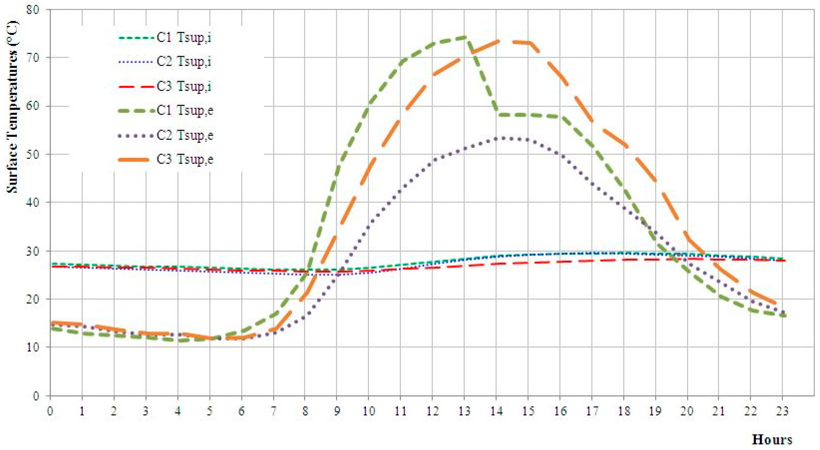
The monitored data are useful to characterize the roofing systems also as regards the thermal wave phase shift (φ), in terms of the period of time in which the thermal wave flows from the outside to the inside through a building material, and damping or attenuation phenomena. Figure 5 shows the graphic image of the thermal wave phase shift from the summer monitoring data, dated 26 July 2015, in passive operating system.

Table 6. Thermal wave phase shift and attenuation as a function of the monitored data.

	Phase Shift	Attenuation
	(Hours)	°C	%
C1	5	45 ca	60
C2	3	24 ca	45
C3	6	45 ca	61.5

shows data relating the calculation of thermal wave phase shift and attenuation.

C3, which houses the vented-roof, has the highest phase shift value, thanks to the vented cavity that mitigates the effects of the global solar radiation and adapts to the trend of the external temperature. In contrast, C2 has the smallest value of phase shift because the reflective properties induce a peak surface temperature significantly lower than the other roofing systems (about 20 °C less), and therefore a considerable reduction of the thermal load that is transmitted by conduction. Hence a lower phase shift of C2 also with respect to C1, that shares the same type of construction, except for the reflective surface finish.

C1 stores the same surface heat of C3 but it does not benefited from the inside natural ventilation; therefore presents a balanced value between C2 and C3.

As regards the thermal wave attenuation, C1 and C3 show very similar results, although with C3 performing slightly better; C2 shows the smallest value of attenuation.

3.1.3. Verification of Cool Roof Performance Deterioration after One Year

One of the most sensitive issues concerning the use of a cool roof is related to the performance deterioration [48], generally expected within the first three years from the installation [25], due to the natural fouling process caused by environmental and anthropogenic pollutants which reduce the reflecting properties of the finishing materials.

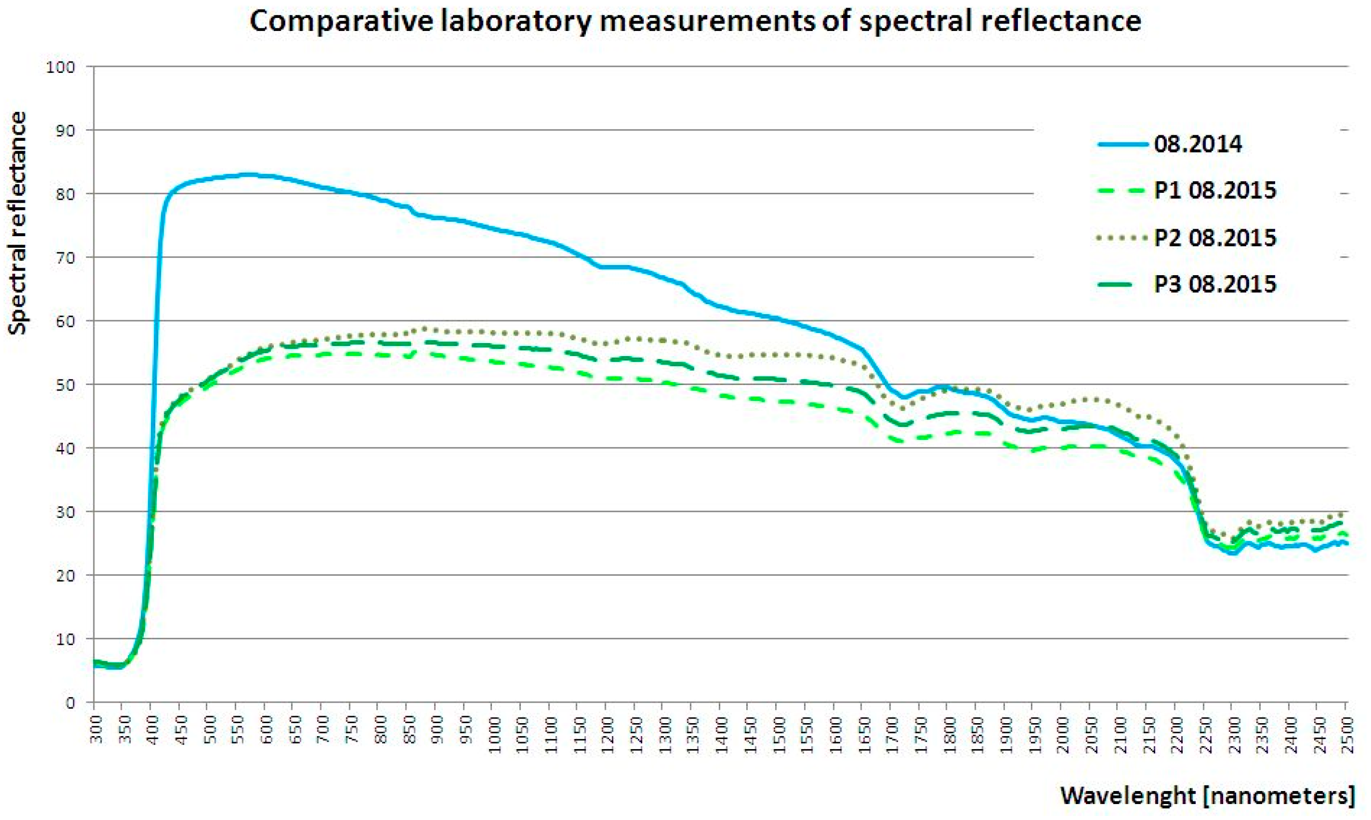
Through the analysis and comparative study on the months of August 2014 and August 2015 relating to the C2 monitoring data, a numerical evaluation—in terms of surface temperature gradient—of this decay was possible. The analysis was carried out with similar global solar radiation belts and external temperatures.

Table 7. Tables comparing August 2014 and 2015 data, Solar Radiation 800–900 W/m².

	August 2014 Peak Values				August 2015 Peak Values
I 700–800 W/m2	10	11	14	29	09	18	21	22	26	28	29	30	31
RSG (W/m2)	830	810	771	754	809	759	795	834	804	790	781	793	814
Tex (°C)	33	32	28	30	35	29	30	31	32	34	36	36	36
Tsuravg C2 (°C)	41	43	38	40	54	50	47	50	50	52	53	54	53

Notes: solar radiation—I; Global Solar radiation—RSG, external temperature—Tex, C2 surface temperature, average value—Tsuravg C2.

and

Table 8. Comparison of peak values, Solar radiation 500–600 W/m².

	August 2014 Peak Values				August 2015 Peak Values
I 500–600 W/m2	03	21	25	28	15	19	27
RSG (W/m2)	594	608	580	601	558	728	634
Tex (°C)	28	28	24	27	28	29	31
Tsuravg C2 (°C)	30	39	32	36	37	47	50

Notes: solar radiation—I; Global Solar radiation—RSG, external temperature—Tex, C2 surface temperature, average value—Tsuravg C2.

shows tabulated data related to the monitoring of the indicated physical dimensions for different solar radiation belts.

As shown by the monitoring data, after one year with the same outdoor conditions, the C2 external surface temperature increased from approximately 42–44 °C to 50–51 °C, with a minimum temperature gradient equal to 7 °C.

The experimental results led to replication of the laboratory tests for the determination of both the spectral and integrated reflectance [44]. Figure 6 shows the comparison between the initial spectral reflectance curve of the Canadian style tiles coated with high solar reflectance coating and the same curves after a year of exposure to weather and outdoor pollutants.

Given the above fouling conditions, the laboratory tests were conducted at three different points of the tile sample, corresponding to the three curves in green: the decay of the reflective performance compared to August 2014 are graphically net and sensitive. The calculation of the relative absorption coefficient is equal to 0.5 which, compared to the laboratory value of 2014 equal to 0.92, shows a loss of approximately 46%, which is far beyond expectations. The data available in the literature, as well as those provided by the manufacturer, report a loss of about 10%–20% after two years of outdoor exposure [25].

This is easily explained by some particular aspects of the experimental set-up: the test cell is reduced in height and is located close to a busy road in an industrial area south of Milan. Therefore, even though the roofs are pitched by 30° so as to favour ‘self-cleaning’, they are undoubtedly exposed to a level of pollution and dirtying not comparable to the real service conditions of a building, or worse to the conditions of laboratory aging. However, such sharp experimental data justify the highlighted variation of the monitored surface temperatures.

3.2. Assessment of the Indoor Thermal Comfort

The analysis of the hygrothermal indoor comfort level in the three cells under study is addressed over the different seasons in passive conditions, except for a tower fan that prevents the vertical stratification of the indoor air temperature. Passive conditions allow making a comparative assessment of the contribution of reflective paint in different seasons.

The UNI EN ISO 7730 [49] allows for the analytical determination of the hygrothermal well-being of an indoor environment through two indices, the PMV (Predicted Mean Vote) and PPD (Percentage of People Dissatisfied) by providing a framework of internal environmental conditions deemed acceptable and satisfactory, and an interpretive approach of any local discomfort. The calculation of the PMV and PPD was carried out by direct comparison between pairs of cells: C1–C2, C2–C3, and C1–C3.

The annual analysis has revealed the following:

• the winter season is the boundary condition for external temperature, relative humidity and solar radiation level, where the typological features of the three roofing systems tend to flatten in such a way that no substantial performance difference is highlighted;
• during the intermediate seasons, spring and autumn, C1 showed the best performance, while roofing system C3 showed an overall negative performance of the experimental set-up. In the intermediate seasons C2 significantly improves the performance of a vented-roof, as well as that of a warm-roof only at the solar radiation peaks. C2, however, being characterized by a low value of thermal wave phase shift, shows a worse performance at night, albeit not very considerable;
• during the summer season, the roof with the best performance is C3, thanks to the action of heat removal due to ventilation in the air gap. C2 significantly improves performances compared to C1, confirming the known outcomes of the tests.

As regards the relative humidity values, C2 is the most negatively affected, even if, except for the winter season, the differences with respect to C1 (about 10%) and C3 (about 5%) are reduced.

3.3. Assessment of the Energy Consumption

The main goal of the consumption analysis is to compare the energy performances of the three roof systems under study with each other, on a seasonal basis. The three experimental set-ups have the same structural characteristics and orientation, and house the same heating/cooling equipment. Therefore, the difference in energy consumption reflects the specific behavior of the roofing systems, which does not depend exclusively on the overall thermal transmittance value (such datum is interesting in itself considering the discrepancies between the values calculated according to the standard and the values obtained from the on-site heat flow meter monitoring). The difference between the energy consumptions also depends on specific characteristics, such as the ability to reflect solar radiation (C2) or on the ventilation in the cavity (C3).

The energy analysis is carried out in terms of: cumulative energy consumption as a function of the cumulative degree-hour and the power delivered as a function of solar radiation.

3.3.1. Summer Energy Consumption for Cooling

The analysis of C2 summer energy consumption is performed by comparing the monitoring results related to the summer of 2014 and of 2015: inasmuch as the level of fouling, and the ensuing performance deterioration of reflective properties, may be greater than realistically expected due to the specific features of the experimental set-up, however, they provide the reference boundary parameters on the expected performance on site.

Table 9. Cooling periods and weather data. The period of diurnal average of solar radiation is from 7 a.m. to 6 p.m.

Configuration	Period	External Temperature (°C)			Solar Radiation (W/m2)
		Min	Max	Avg	Max	Avg
(a) Cooling 2014	1–31 August	14.72	33.12	23.47	919	424
(b) Cooling 2015	1–31 August	16.92	38.74	25.74	894	436

Notes: external temperatures: minimum—Min, maximum—Max, average—Avg; solar radiation: maximum—Max and average—Avg.

shows an overview of the main features of the two summer monitoring periods.

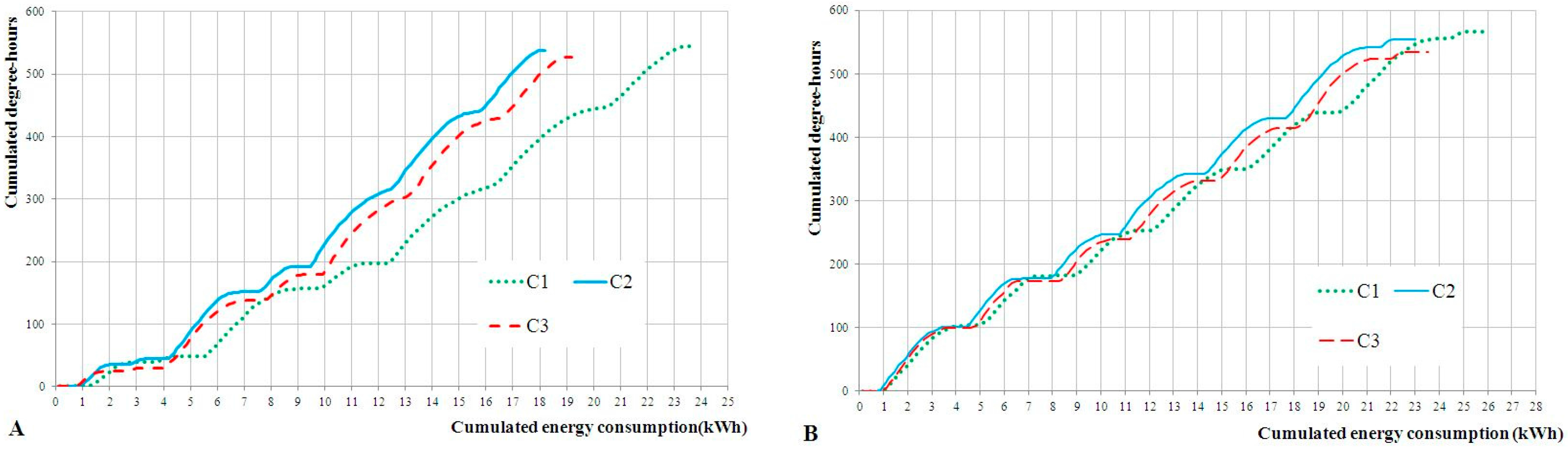
Figure 7 shows the plots of the cumulated consumption as a function of the cumulated degree-hours for two weeks of reference, ‘A’ representative of the period (a) from 25 to 31 August 2014, and ‘B’ for the period (b) from 17 to 23 August 2015.

The analysis of the graphs relating to the reference weeks for 2014 and 2015 shows that the consumptions of C2 are lower both with respect to C1 (worst performance) and to C3, which confirms the expectations. However, the comparison points out, though still confirming the approximate trends, that the fouling phenomena involve a flattening of consumption data, dramatically reducing the percentage savings, as shown in

Table 10. Energy consumptions: percentage gradients with respect to C1.

	C1	C2	C3
Energy Consumption (a) (kWh)	23.5	18.3	19.3
Gradients (a) (%)	–	−22.1	−17.8
Energy Consumption (b) (kWh)	26.2	23.2	23.8
Gradients (b) (%)	–	−11.4	−9.1

.

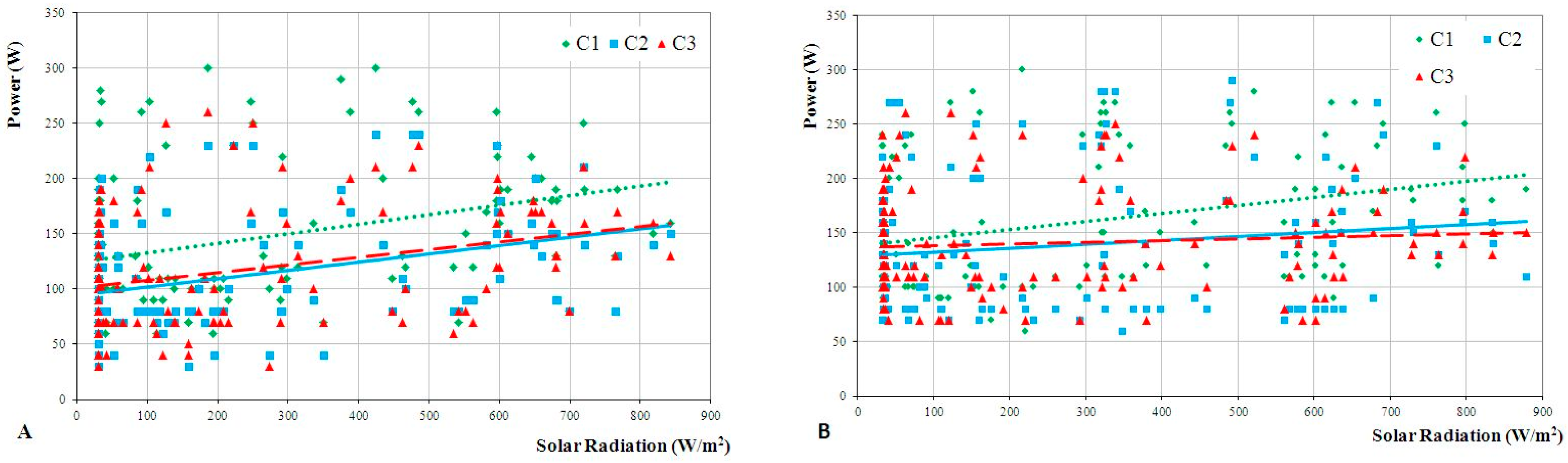
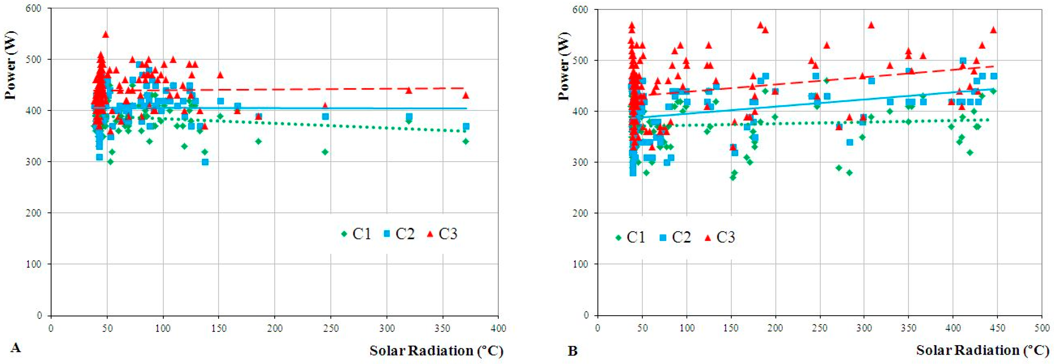
Flattening in consumptions becomes even more clear in the light of the data relating to the power outputs as a function of external radiation for the corresponding weeks (Figure 8).

Figure 8B, concerning configuration (b), highlights how C2 and C3 reverse their behavior at a very low solar radiation level, by about 400 W/m². The loss of reflective capacity of the C2 roofing system, already underlined when analyzing external surface temperatures, is further confirmed by the generated power.

However, because the reflective performance loss observed in the laboratory (46%) is more than double with respect to the expected limits [48], in the case of routine maintenance and cleaning, the summer performance of a cool roof compared to a traditionally vented-roof is always to be considered improved.

3.3.2. Winter Energy Consumptions

The analysis of winter energy consumptions was developed considering monitoring data of the 2015/2016 winter (from 21.12.2015 to 21.03.2016), because the 2014/2015 winter season (from 21.12.2014 to 21.03.2015) was dedicated to the study of the performance of the three roofing systems in passive conditions. Two different winter season weeks are proposed; the former is characterized by atmospheric disturbances, the latter by sunny weather, to better compare energy behaviors.

Table 11. Heating periods and weather data. The period of daytime average of solar radiation is from 10 a.m. to 3 p.m.

Configuration	Period	External Temperature (°C)			Solar Radiation (W/m2)
		Min	Max	Avg	Max	Avg
(a) Heating 2016	4–10 January	−1.14	8.48	2.91	428	151
(b) Heating 2016	11–17 January	−1.26	13.92	5.11	445	249

Notes: external temperatures: minimum—Min, maximum—Max, average—Avg; solar radiation: maximum—Max and average—Avg.

shows an overview of the main external environment characteristics concerning the chosen representative winter season weeks.

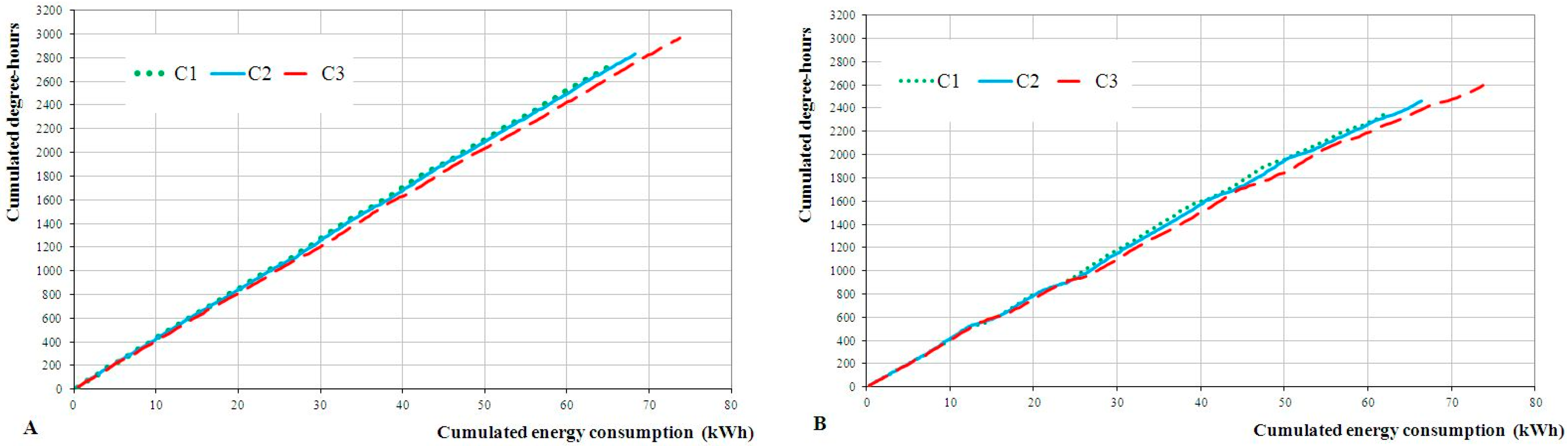
Figure 9 shows graphs concerning cumulative consumptions as a function of cumulated degree-hours for the two reference weeks, (a) of Table 10, and (b) of Table 10.

From the analysis of the graphs it is possible to highlight some very interesting aspects concerning the energy behavior of three roofing systems during the winter season. First of all: C3 is the solution with the highest heating consumptions. C1 and C2 are quite similar. The comparison data between C1 and C2 are more interesting in view of the fact that, however a marked performance deterioration occurred during the winter 2015/2016 as far as the C2 roof is concerned, the reflectance value of the roofing is 0.5, which is clearly greater than 0.29, as found with the Canadian type tile of C1 and C3.

In the second place, the difference in consumption (

Table 12. Energy consumptions: percentage gradients with respect to C1.

	C1	C2	C3
Energy consumption (a) (kWh)	65	68	75
Gradient (a) (%)	–	4.6	15.4
Energy consumption (b) (kWh)	62	65	73
Gradient (b) (%)	–	4.8	17.7

) between the week (a) characterized by six days of overcast sky and rainfall, compared to the week (b) characterized by five days of clear skies and a good level of solar radiation, is considerable even though the patterns are similar. The drop in consumption between the two weeks was due to the weather characteristics and only limited to the reflective capacity of C2.

The trend outlined by the analysis of energy consumption is even more pronounced in the analysis of the power supplied as a function of solar radiation, as shown in Figure 10.

The graphs confirm the consumption patterns: C1 has the lowest requirement for power output, while C2 shows significantly better performance compared to C3. However, the graphically displayed data which graphically appear is the deviation of the trend and the increase of the power output of C2 compared to C1 with the increase of the direct solar radiation level, as emphasized by Figure 9B, by the action of the high-reflectance paint.

4. Conclusions

The main goal of the present research is the comparative assessment of the behavior of a cool roof solution with respect to a vented-roof and a warm-roof both in summer and in winter seasons, through an experimental campaign carried out in three outdoor test cells. The climate context is the zone E according to the Italian legislation in force [40], ‘Cfa’ for the Koppen-Geiger climate classification [41].

The majority of the studies mentioned in the literature concerning cool roofs are focused on their contribution to the mitigation of the UHI phenomenon though global climate models, or highlight the benefits they provide in summer.

Some studies are focused on the energy behavior in winter too, calculating heating penalty due to the solar heat loss by reflection. The majority of those researches calculates the increased heating demand through energy and microclimatic simulations [21,28,31,33,36,38]; some authors, such as Kolokotroni et al. [33], Stavrakakis et al. [38] and Pisello et al. [37] have performed on-site monitoring of some variables mainly to validate the building simulation model. Finally, some researches analyse the energy performances of cool roofs though a comparative assessment with respect to green roofs [28], or balance cooling savings with the increasing of the heating consumptions in winter [28,35].

The presented study, instead, is completely based on an on-site monitoring campaign in outdoor test cells which lasted two years and compares summer and winter behavior of a cool roof solution with respect to the two most common roofing technologies in northern Italy, warm-roofs and vented-roofs, under working conditions. The research has also considered the cool roof performance deterioration after one year and its effect on the roof energy performances and the external surface temperatures.

Based on these initial assumptions, the results obtained allow for drawing the following conclusions:

• From the point of view of energy consumptions, the cool roof allows to reach the maximum level of savings (approximately 20%) with regard to the summer air conditioning, also related to a vented-roof, in which the ventilation in the cavity, by removing part of the heat transmitted toward the lower surface of the roofing by conduction and radiation, already significantly improves performance compared to a warm-roof; as regards, instead, the winter season, the cool roof has a slightly worse performance with respect to a warm-roof (<5%) and a significantly better one if compared to a vented-roof (>12%);
• From the point of view of thermo-hygrometric indoor comfort, the winter season is the ultimate condition where a flattening of the typological features of the three coverage systems occurs, yet without producing any remarkable difference in performance; during intermediate seasons, the cool roof significantly improves performance compared to both a vented-roof and a warm-roof only at the solar radiation peaks. The reduction by reflection of the amount of absorbed solar radiation, leads to a barely noticeable reduction of the free solar gains and thus to a worse performance at nighttime (reduced thermal wave phase shift); finally, during the summer season, the cool roof involves a significant improvement in performance compared to the warm-roof, confirming the known outcomes of the tests. As regards the relative humidity values, C2 is the most negatively affected, even if, except for the winter season, the differences compared to the warm-roof (about 10%) and to the vented-roof (about 5%) are quite small;
• From the point of view of the characterization of the roofing system, the cool roof, by acting directly on the albedo value, allows a significant reduction in surface temperatures as a function of the solar radiation level, according to values equal to 15–20 °C in the summer season and about 10–15 °C in the winter season for solar radiation levels exceeding 600 W/m²; while, on an annual basis, for radiation levels lower than 200 W/m² the value is equal to 3–7 °C. Furthermore, results confirm a strong reduction in surface peak temperatures, which amounted to about 30–60 °C for the cool roof compared to 58–75 °C of the roof with Canadian tiles.

Therefore, the experimental data suggest that the cool roof are appropriate solutions to sensibly improve summer energy performances without any appreciable negative impact during winter in temperate climates, and to positively contribute to the mitigation of the heat island effect.