Rough Set Theory for Real Estate Appraisals: An Application to Directional District of Naples

Abstract

This paper proposes an application of Rough Set Theory (RST) to the real estate field, in order to highlight its operational potentialities for mass appraisal purposes. RST allows one to solve the appraisal of real estate units regardless of the deterministic relationship between characteristics that contribute to the formation of the property market price and the same real estate prices. RST was applied to a real estate sample (office units located in Directional District of Naples) and was also integrated with a functional extension so-called “Valued Tolerance Relation” (VTR) in order to improve its flexibility. A multiple regression analysis (MRA) was developed on the same real estate sample with the aim to compare RST and MRA results. The case study is followed by a brief discussion on basic theoretical connotations of this methodology.

1. Introduction

Common methods for data prediction require assumptions or parameters unrelated to observed phenomena, or presuppose that properties have quantitative characteristics and are subject to random effects, so that statistical methods may be applied, such as multiple regression (parametric or not), variance analysis or correlation [1,2,3,4,5,6,7]. Rough Set Theory (RST) was developed by Pawlak et al. in the early 1970s [8,9,10,11] and has received wider attention in many research fields as a means of data analysis [12] but only very marginally in the real estate sector [13,14,15,16]. The basic assumption of RST is that information is presented and perceived with granularity: “The information about a decision is usually vague because of uncertainty and imprecision coming from many sources...Vagueness may be caused by granularity of representation of the information. Granularity may introduce an ambiguity to explanation or prescription based on vague information” [17].

Unlike other methods, the original Rough Set approach uses only the knowledge presented by data itself and does not rely on statistical parameters and assumptions external to the analysis.

In other words, RST is based on the hypothesis that some objects are indiscernible from others if they are classified in the same way according to their associated information; thus, the concepts of indiscernibility relation, upper and lower approximation, and accuracy of the approximation are considered in RST [11,18,19,20,21,22,23,24].

However, the original version of RST as valuation methodology has limitations.

Although the rules on which RST is based allow one to appraise a property using a relation less strong than econometrical models, the main issue is that in many cases the values need to be crisp, while RST in its original version offers only value intervals. For these reasons, more recent studies have begun experimenting an integration of RST with a functional extension that represents a more flexible way to deal with the indiscernibility relation (Value or Valued Tolerance Relation, VTR) [14,15].

Main aims that encourage the use of RST include the ability to operate with small comparison samples or in all cases where the econometric modeling of market prices is too complex. In fact, the lack of comparison data inhibits the use of possible and alternative comparison methods or adds uncertainty to real estate appraisals.

Problems on uncertainty are deeply rooted in the real estate field. Each real estate market is unique given the specific features of real estate properties (e.g., variation in physical features, diversity of legal titles, etc.) and of the relative market (e.g., lack of uniformity, high imperfection, low efficiency, and transparency), as well as behaviors of actors in the real estate market that lead to a higher imperfection of property valuations as compared to other assets.

Larr and Riebe [25], Mallinson and French [26], Ekelid et al. [27], Young [28], and many others argue in favor of a range of values for overcoming uncertainty in real estate appraisals: “Since appraisals are a combination of current fact and future expectations, relying on only one value indicates an unsupported confidence in both the appraisal process and the appraiser. […] Valuation models should be adjusted to accept a range of likely projections and then used to provide a range of value within one standard deviation” [25]. Adair and Hutchinson [29] take a different approach instead; they suggest risk scoring to report the level of risk within property pricing. In a similar way, other instruments from risk analysis could be used, such as scenarios in combination with confidence intervals, real option analysis [30], or Monte Carlo simulations [31]. Therefore, the challenge is to improve the output of an appraisal in just the right way, possibly with the help of qualitative or quantitative instruments known from the strategic management literature [32].

That said, RST is closer to the point of view that suggests a range of values for overcoming uncertainty in real estate appraisals.

In this paper, in order to overcome shortcomings of RST, the application to a case study of RST was tested with the aid of a VTR tool. Additionally, a multiple regression analysis (MRA) was developed on the same real estate sample with the aim to compare RST and MRA results.

2. Rough Set Theory: Original Idea and Analytical Aspects

Rough Set is an evaluation methodology characterized by a Boolean math structure, initially applied as a decision support tool under uncertainty conditions [17]. It finds a wider application in the analysis of medical data and in the economic field [12], where RST allows one to rank a large number of observations and performs the resulting deductive analysis on the same sample (cause–effect analysis).

The tabular analysis, on which RST is based, is reported as follows (see Figure 1): the rows identify the objects (observations), while the columns are representative of attributes (characteristics or modalities hired by objects).

RST assumptions are the following:

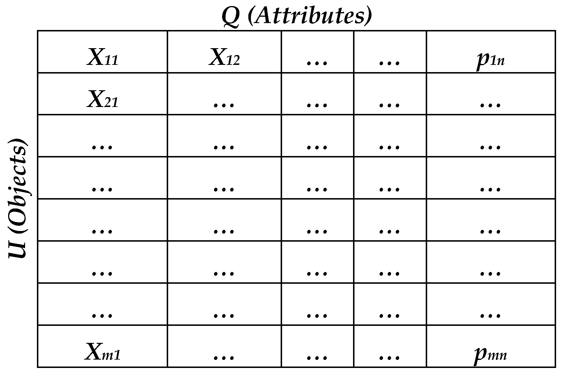
• $S=\langle U,Q,V,\rho \rangle$ is an information system, where U is a finite set of objects, Q is a finite set of attributes, $V=U_{q\in Q}{V}_q$ being V_q a domain of q attribute, and $\rho :U\times Q\to V$ is a function such that $\rho \left(x,q\right)\in V_q$ for every $q\in Q$ and $x\in U$.
  $P\subseteq Q$ and $x,y\in U$: x and y are considered as indiscernible objects by the set of attributes P in S if $\rho$ (x,q) = $\rho$ (y,q), for every $q\in P$.
  The elementary groups of P relationships are defined as equivalence classes in S.
  Essentially, two objects with similar attributes fall in the same equivalence class and are considered indiscernible.
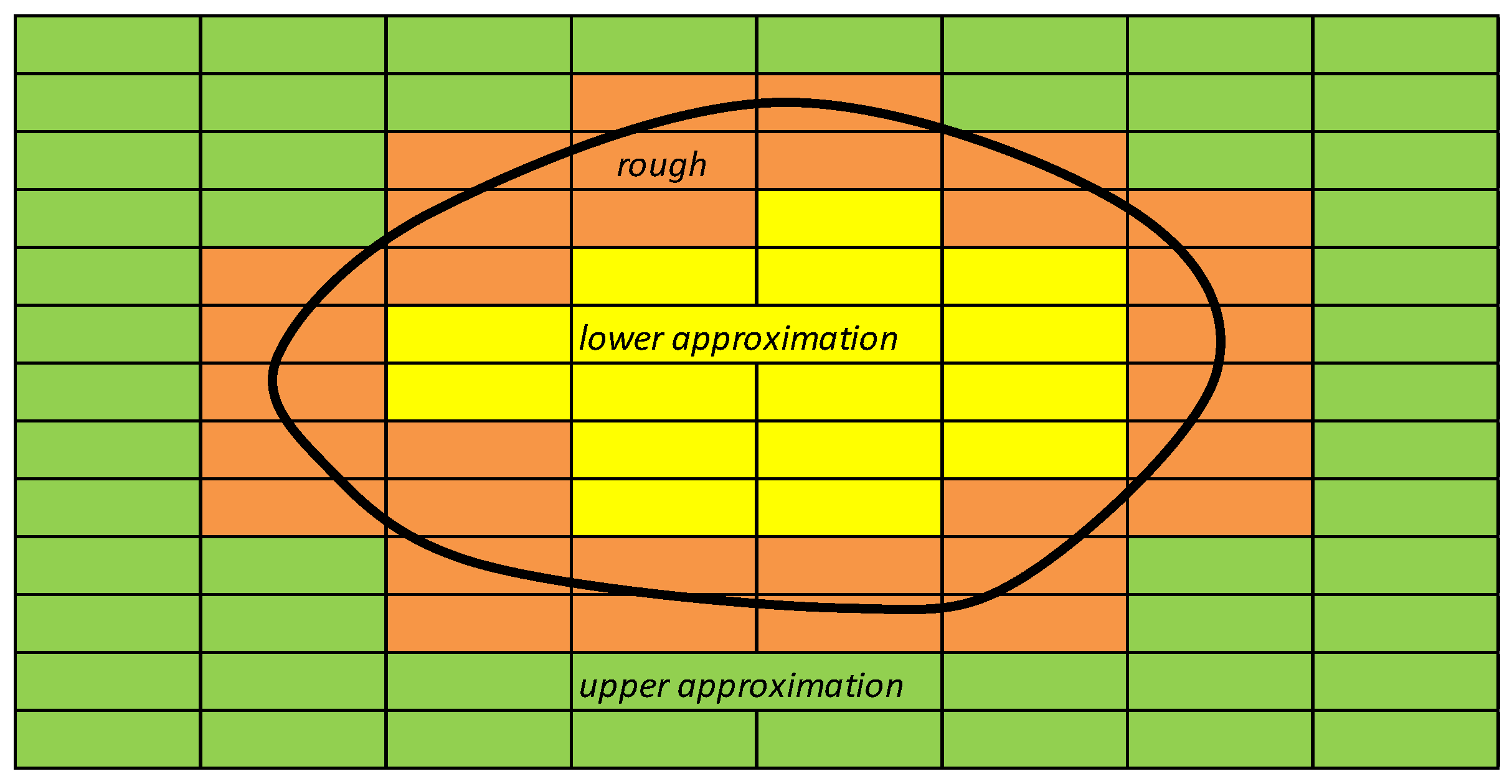
• Two types of attributes exist: “conditional” attributes represent the observations; “decisional” attributes represent the “judgments” detected or assigned for the overall set of conditional attributes, with reference to the specific object.
  If conditional attributes are equal but decisional attributes are different, the set of objects comes to be in a “rough” region (see Figure 2).
  The objects that may be distinguished are inserted in different equivalence classes, identified by approximations. Every equivalence class is identified by upper and lower approximation regions.
  For $P\subseteq Q$ and $Y\subseteq U$, $\underset{\_}{P}Y$ is defined as the lower approximation of Y and $\overline{P}Y$ as the upper approximation of Y:

  $$\underset{\_}{P}Y= \left\{X\in P^{*} and X\subseteq Y\right\}$$

  (1)

  $$\overline{P}Y= \left\{X\in P^{*} and X\cap \text{}Y\ne 0\right\}$$

  (2)

  where P* represents the family of all equivalence classes for each P relationship in U.
  The lower approximation $\underset{\_}{P}Y$ represents the set of elements U “certainly” included in Y, applying the set of conditional attributes P; the upper approximation $\overline{P}Y$ represents the set of elements U that “if possible” is included in Y, applying the same set of attributes P.
  The relationship between number of elements of the lower approximation and number of elements of the upper approximation is defined as “accuracy” of approximation:

  $${\mu }_p\left(Y\right)=\frac{card\left(\underset{\_}{P}Y\right)}{card\left(\overline{P}Y\right)}$$

  (3)

  It also defines as “quality” of approximation’s classification the following relationship:

  $${\gamma }_P\left(X\right)=\frac{{{\displaystyle \sum }}_{i=1}^{n}card\left(\underset{\_}{P}{Y}_i\right)}{card\left(U\right)}$$

  (4)

  where card(U) represents the total number of elements (objects) included in the set of observations U, n is the number of modalities (or classes) of conditional attribute, and $card\left(\underset{\_}{P}{Y}_i\right)$ is the number of objects contained in each lower approximation of the various classes n.
  The quality classification expresses synthetically the relationship between the numbers of correctly classified objects respect to the total number of objects.
• The choice of the equivalence class is performed by “if then” rules, rules that are measured in terms of “precision” and “coverage” in relation to analyzed objects. The “precision” defines the rule (“if”) and identifies the objects, while “coverage” detects the fraction of objects that responds positively to the rule (then).
• The best rule is, precisely, defined as that which provides the best coverage (better generalization capacity).

3. Rough Set Theory Applied to Real Estate Appraisals

In the real estate field, RST allows one to determine a property value by “if then” rules, which create a logical link between the characteristics of a real estate unit and its market price.

The procedure was first applied in support assessments to urban and regional planning and, more recently, it was tested for mass appraisal purposes also with reduced availability of comparison data or when difficulties in the econometric modeling of market prices were detected.

During application of RST methodology, the individual transactions that characterize a real estate market segment are the objects in a universe that contains the totality of transactions.

Each exchanged properties has characteristics that determine the attributes (conditional) of an object.

The relationship between objects and attributes are identified in the methodology through the following lexical diagnosis: “certainly,” “possibly,” and “certainly no.”

Two objects or properties that appear to be similar with regard to their technical characteristics, located in comparable positions and with the same market price, may be considered “indistinguishable.”

The description of the relations between object and attributes or between observed property and its characteristics is methodologically developed, as previously indicated, by a double entry table (also called “information table,” see Figure 1).

In the application of the methodology, it is assumed that for each object an exact measurement (error-free) of each attribute with reference to a given time instant is feasible.

The choice of the attributes relating to the object is comparable to the selection of the explanatory variables in the regression process usually used for real estate appraisals.

A further relevant principle of the Rough Set methodology is that, in the absence of specific knowledge, all the relationships between the object and attributes are “equiprobable.” It should be emphasized that the choice of attributes with low significance makes the “if then” rules unreliable.

For example, given a universe of transactions, two properties (or objects) that present a retail area of 100 square meters are indiscernible with respect to the “area” attribute. This also applies in the presence of more than one attribute, and has great importance for development of “if then” rules on which the formulation of a real estate value judgment is based.

In Rough Set methodology, two properties may differ in only one characteristic while presenting a very different market price. Conversely, the two properties may differ in two or more characteristics but have a similar market price.

As mentioned earlier, if a property (object of transactions universe) has a given characteristic or attribute, it falls within the “positive region” or “lower approximation” of the same object; if only some of the universe objects possess that particular characteristic, the relationship between object and attribute is described by “upper approximation”.

The difference between two regions, corresponding to lower and upper approximations, concurs to qualify the object, identifying the cases in which the attributes that qualify the object are always within the lower approximation or upper approximation.

The description of an object in a real estate appraisal is normally aimed at a determination of its market value.

For this reason, the “information table” must be transformed into a “decisional table”, in which the attributes that constitute the “conditional” part (if) of the rule are distinguished by the “decisional” attribute (market price of property contained in “then” part of the rule).

In this way, it establishes a causal relationship between conditional attributes and the decisional attribute, which excludes every econometric formalization.

The last phase of application of Rough Set methodology is based on the study of existing relationship between conditional and decisional attributes.

These relations are analyzed in light of lower or upper approximations existing between the decisional set (real estate market prices) and the set of attributes selected for the conditional part of the rule.

If a set contains the objects with the same decisional attribute (properties that have the same price or that fall in the same price class), it encloses all objects that belong to the same set of conditional attributes (retail area or other characteristics); there is a “deterministic” rule between conditional and decisional parts of the rule that, in rough terms, is represented by the coincidence of lower and upper region approximation.

The universe of objects can also generate approximate rules, but the few experiments on RST performed in the real estate field suggest the use of deterministic rules only [13,14,15].

4. Case Study: Application of RST to Directional District of Naples

The application that follows was carried out using ROSE2 software [22,23,24].

The data sample refers to a defined real estate market segment of Naples and, specifically, n. 30 real estate transactions related to office units located in the Directional Centre during the first semester of the year 2016 (

Table 1. Real estate data.

No.	Area (m2)	Maintenance	Parking Space	Price (€)	Price Class
1	51	1	0	60,828	1
2	53	0	0	71,315	1
3	55	0	0	79,705	1
4	60	1	0	79,705	1
5	60	0	0	79,705	1
6	60	0	0	79,705	1
7	50	1	0	82,222	1
8	65	0	0	82,222	1
9	55	0	0	92,290	2
10	58	0	0	92,290	2
11	60	0	1	96,485	2
12	50	1	1	100,680	2
13	55	0	1	100,680	2
14	50	0	1	109,070	2
15	54	0	1	113,265	3
16	52	0	1	113,265	3
17	80	0	1	117,460	3
18	65	0	0	117,460	3
19	80	0	0	125,850	3
20	62	0	0	125,850	3
21	60	1	0	142,630	3
22	67	0	1	151,020	3
23	90	1	1	159,410	3
24	60	0	1	167,800	4
25	108	0	1	226,530	5
26	110	0	1	234,920	5
27	120	0	0	236,598	5
28	120	1	0	251,700	5
29	140	0	1	251,700	5
30	140	1	1	268,480	5

and

Table 2. Statistical description of the real estate data.

Description	Area (m2)	Maintenance (m2)	Parking Space (m2)	Price (€)
Std. Deviation	27.63	0.45	0.51	62,400.24
Median	60.00	0.00	0.00	113,265.00
Average	73.00	0.27	0.47	133,694.65
Min	50.00	0.00	0.00	60,827.50
Max	140.00	1.00	1.00	268,480.00

).

The sampled properties have the same build type and quality (units located in office towers recently built), and they are included in a homogeneous urban area in terms of qualification and distribution of main services. For these properties, the following characteristics as conditional variables (conditional attributes) were recognized: commercial area (measured in m²), presence/absence of parking space (represented by a dummy variable: 1 = if present, 0 = if absent), and maintenance status (represented by a dummy variable: 1 = if office unit was recently renovated featuring luxury finishes, 0 = if office unit has a normal state of maintenance). The market price (in euros) is the decisional variable (decisional attribute).

The statistical description of the real estate data is reported in Table 2.

Direct knowledge of the local real estate market helped to identify five price classes assuming, for the first two classes, a maximum difference between minimum and maximum prices recorded equal to €25,000, while for the other classes a maximum difference of €50,000 was considered. These price classes have been defined taking into account, as much as possible, of the similarity degree between office units (in terms of real estate characteristics detected).

The real estate data have been reported in

Table 3. Price classes.

Price Class	Min	Max	Difference
1	60,000	85,000	25,000
2	85,000	110,000	25,000
3	110,000	165,000	50,000
4	165,000	210,000	50,000
5	Over 210,000		-

.

The conversion of the decisional attribute, from punctual element to price classes, derives from the fact that the first—with continuous numerical representation—does not provide significant indications in the procedure, as it does not allow one to identify, precisely, those similarities able to carry out the generalization of synthesis, which is at the basis of RST.

In this way, it is possible to identify the equivalence classes that represent the sets of similar properties in terms of conditional attributes, as shown in

Table 4. Equivalence classes.

List of equivalence classes in which conditional attributes have equal modalities

{1}; {2}; {5, 6}; {7}; {10}; {12}; {13}; {14}; {15}; {16}; {17}; {19}; {20}; {22}; {23}; {25}; {26}; {27}; {28}; {29}; {30}; {3}; {4}; {8}; {9}; {11}; {18}; {21}; {24}.

.

The high dispersion of equivalence classes is a symptom of the difficulties of generalization, constituting, this, a paradigmatic case of “rough” extensive region.

To determine a system of rules that identify a logical link among characteristics and decisional attribute (market price), first the lower and upper approximations of each decisional class must be known; then, a set of rules that are usable for the formulation of a judgment on the property value are needed.

For this aim, it is possible to define the lower and upper approximations for each price class as shown in

Table 5. Lower and upper approximations for Price Class 1.

LOWER APPROXIMATION CLASS 1: all objects that are indistinguishable as well as having a price belonging to Class 1	{1}; {2}; {5, 6}; {7}.
UPPER APPROXIMATION CLASS 1: all objects that may belong to Class 1	{1}; {2}; {5, 6}; {7}; {3}; {9}; {4}; {21}; {8}; {18}.
Number of objects in the class: 8
Number of objects in the lower approximation: 5
Number of objects in the upper approximation: 11
Accuracy: 0.4545

,

Table 6. Lower and upper approximations for Price Class 2.

LOWER APPROXIMATION CLASS 2: all objects that are indistinguishable as well as having a price belonging to Class 2	{10}; {12}; {13}; {14}.
UPPER APPROXIMATION CLASS 2: all objects that may belong to Class 2	{10}; {12}; {13}; {14}; {3}; {9}; {11}; {24}.
Number of objects in the class: 6
Number of objects in the lower approximation: 4
Number of objects in the upper approximation: 8
Accuracy: 0.5000

,

Table 7. Lower and upper approximations for Price Class 3.

LOWER APPROXIMATION CLASS 3: all objects that are indistinguishable as well as having a price belonging to Class 3	{15}; {16}; {17}; {19}; {20}; {22}; {23}.
UPPER APPROXIMATION CLASS 3: all objects that may belong to Class 3	{15}; {16}; {17}; {19}; {20}; {22}; {23}; {4}; {21}; {8}; {18}.
Number of objects in the class: 9
Number of objects in the lower approximation: 7
Number of objects in the upper approximation: 11
Accuracy: 0.6364

,

Table 8. Lower and upper approximations for Price Class 4.

LOWER APPROXIMATION CLASS 4: all objects that are indistinguishable as well as having a price belonging to Class 4
UPPER APPROXIMATION CLASS 4: all objects that may belong to Class 4	{11}; {24}.
Number of objects in the class: 1
Number of objects in the lower approximation: 0
Number of objects in the upper approximation: 2
Accuracy: 0.0000

and

Table 9. Lower and upper approximations for price class 5.

LOWER APPROXIMATION CLASS 5: all objects that are indistinguishable as well as having a price belonging to Class 5	{25}; {26}; {27}; {28}; {29}; {30}.
UPPER APPROXIMATION CLASS 5: all objects that may belong to Class 5	{25}; {26}; {27}; {28}; {29}; {30}.
Number of objects in the class: 6
Number of objects in the lower approximation: 6
Number of objects in the upper approximation: 6
Accuracy: 1.0000

.

From Table 5, Table 6, Table 7, Table 8 and Table 9, it is clear that Price Class 5 is an exact set because the upper and lower approximations have overlapping sets (“not rough”).

Based on the indicated lower approximations, it is possible to determine the rules that allow one to develop the appraisal by Boolean logic.

Deterministic rules allow one to identify the property price class without any econometric formalization, through rules that establish a logical relation between property price (decisional attribute) and its characteristics (conditional attributes):

• IF Area = (51, 53) → Price Class = 1;
• IF Area = 50 ˄ Park = 0 → Price Class = 1;
• IF Area = 60 ˄ Maintenance = 0 ˄ Park = 0 → Price Class = 1;
• IF Area = 58 → Price Class = 2;
• IF Area = (50, 55) ˄ Park = 1 → Price Class = 2;
• IF Area = (80, 54, 52, 62, 67, 90) → Price Class = 3;
• IF Area = (120, 140, 108, 110) → Price Class = 5;
• Can also to be defined the “approximate” rules, which are a specificity of RST:
• IF Area = 55 ˄ Park = 0 → Price Class = 1 OR 2;
• IF Area = 60 ˄ Maintenance = 1 → Price Class = 1 OR 3;
• IF Area = 65 → Price Class = 1 OR 3;
• IF Area = 60 ˄ Park = 1 → Price Class = 2 OR 4.

With the above rules, it is possible to describe uncertain and vague behaviors that are present in the real estate market.

The deterministic rules show that the “maintenance status” variable does not seem to be important. In fact, if a multiple regression analysis is run on the data of Table 1, the t-test of the variable “maintenance status” will be 0.31, while the t-tests of the characteristics “parking space” and “area” will be, respectively, 2.38 and 12.61. As a consequence, the variable “maintenance status” can also be considered unreliable for multiple regression analysis. It should be highlighted, therefore, that starting from the same real estate data, RST and multiple regression analysis arrive to same results.

In the case study, seven deterministic rules and four approximated rules have been generated starting from 30 observations. A real problem is that, if we want to appraise an office unit of 130 m², with parking space and without luxury maintenance status, we do not have the opportunity to apply the rules identified by RST. For this reason, RST may be integrated with a functional extension also called “Value Tolerance Relation” (VTR).

VTR can be considered a flexible tool to deal with indiscernibility relation. In this sense, VTR allows one to develop the upper or lower approximations with different degrees of indiscernibility relation, as indicated by the following equation [15]:

$$R_j\left(x,y\right)=\frac{max\left\{0,min\left[c_j\left(x\right),c_j\left(y\right)\right]+k-max\left[c_j\left(x\right),c_j\left(y\right)\right]\right\}}{k}$$

(5)

where R_j is the VTR that may assume continuous values included in the interval [0, 1], x and y are objects, c_j(x) and c_j(y) indicate the measures of attribute j in the objects x and y, max and min represent the intersection and the union of fuzzy sets, and k is the value threshold to distinguish two objects.

If R_j equals 1, the two objects considered are highly similar, while if R_j equals 0 the same two object are completely different.

Therefore, it derives that two objects x and y may have different levels of indiscernibility depending on a discriminator value threshold (k), which measures the attributes c_j and can be applied for all objects. The relationship between all attributes of an object and the conditional part of the rules is determined by intersection of all comparison sets with the rule. There will be several values of R_j (one for each attribute of object and conditional part of rule), and the minimum R_j will be selected between n comparisons among the attribute of the object and conditional part of the rule:

$$R_j\left(x,y\right)=mi{n}_{j=1}^n\left[R_j\left(x,y\right)\right].$$

(6)

The more recent literature suggests that standard deviation adequately approximates the k-threshold [15] because, if rules of RST concern office units with similar characteristics, then k-threshold is low.

An example of RST integrated with VTR follows, for an office unit of 130 m² with a parking space and normal maintenance status, taking into account the rules that have been determined using RST for real estate data and k-threshold as standard deviation (see Table 2).

Table 10. Results of Rough Set Theory integrated with Value Tolerance Relation.

Object	Area = 130 m2	Maintenance = 0	Parking Space = 1	Rj (Min Rj Rule)	Rule Selected
k-threshold	27.63	0.45	0.51
Rj Rule 1	0.0000	1.0000	0.0000	0	Rule 7
Rj Rule 2	0.0000	1.0000	0.0000	0
Rj Rule 3	0.0000	1.0000	0.0000	0
Rj Rule 4	0.0000	1.0000	0.0000	0
Rj Rule 5	0.0000	1.0000	1.0000	0
Rj Rule 6	0.0000	1.0000	0.0000	0
Rj Rule 7	0.2838	1.0000	0.0000	0.2838

shows the results of RST integrated with VTR, where conditional part of each rule is compared with the office unit to evaluate. RST integrated with VTD has defined the seventh rule as the more suitable for the office unit to appraise.

After the implementation of RST, an MRA was developed on the same real estate data with the aim to compare forecasting performances of RST and MRA.

In particular, MRA has shown an R-squared value of 0.88 and a substantial validity of the model. Thus, the differences between the observed prices and the estimated prices have been carried out. In

Table 11. Comparison between multiple regression analysis (MRA) and Rough Set Theory (RST) in terms of forecasting performances.

Percentages of Errors (MRA)
0%–10%	10%–20%	20%–30%	more than 30%	Mean Absolute Percentage Error
46.67%	23.33%	20.00%	10.00%	14.44%
Percentages of Errors (RST)
0%–10%	10%–20%	20%–30%	more than 30%	Mean Absolute Percentage Error
50.00%	36.66%	6.67%	6.67%	12.29%

, it can be seen that the mean absolute percentage error and statistics on forecasting errors. The results of the sample’s accuracy about the RST application are also indicated in Table 11, divided for percentage of errors.

For the real estate sample considered the empirical results show the superiority of RST on MRA (the mean absolute percentage error for RST is smaller of 14.89% than to MRA). It must be highlighted that the percentages of errors of MRA, including in the interval 20%–30%, are triple respect to those of RST.

5. Concluding Remarks

This work shows operational potentialities of RST as a valuation methodology. RST was applied to a sample with a low number of variables, and corresponding rules have been generated with the contribution of ROSE2 software.

The results of this paper showed that RST certainly works well with a reduced sample and uncertainty conditions, although this methodology presents some limitation that today again highlight the more flexibility of statistical methodologies commonly used (i.e., multiple regression models, semi-parametric regression, etc.) [33]. However, the relationship between objects and rules in the application of RST for mass appraisal purposes represents a way and a perspective of research partially unexplored yet. In this sense, RST was integrated with the Value Tolerance Relation, a useful tool that improves the flexibility and functionality of RST.

In this paper, RST and MRA are developed on the same real estate sample with the aim to compare their forecasting performances. Some differences between RST and MRA must be highlighted.

Certainly, the greater difference is in the final output. Additionally, RST does not allow one to define information about hedonic-marginal prices. MRA is an econometric model, while in RST the valuation is based on a Boolean product, and the appraiser arrives to the final value estimate looking at the “if then” rule suitable for the object. In the application of MRA, the model will be unreliable if the initial assumptions on errors and on the model are violated. For the application of MRA, different software or tools may be used, while very little software is available for the application of RST. While MRA has a limitation in the number of observations that are required, RST can work also with a small sample; moreover, control indexes are restricted to “accuracy” and “coverage” of rules.

For other aspects, the two methodologies are similar: (a) the applications of RST and MRA are based on a cross-sectional process; (b) the appraisal process starts with the definition of attributes in RST and with the identification of independent variables in MRA; and (c) RST and MRA provide the same results starting from the same sample and attributes.

Applications of RST may be recommended for mass appraisal purposes in those real estate markets with non-transparent conditions, such as in Italy. In addition to forecasting purposes, a further interesting and particular aim for the real estate field could be the use of RST in the boundary areas between contiguous and different territorial areas (homogeneous areas), in order to determine if a property belongs to one or another homogeneous area and to thus resolve conflict situations under uncertainty conditions for real estate market segmentation.

References

1. Del Giudice, V.; De Paola, P.; Forte, F. The appraisal of office towers in bilateral monopoly’s market: Evidence from application of Newton’s physical laws to the Directional Centre of Naples. Int. J. Appl. Eng. Res. 2016, 11, 9455–9459. [Google Scholar]
2. Manganelli, B.; Del Giudice, V.; De Paola, P. Linear programming in a multi-criteria model for real estate appraisal. In Computational Science and Its Applications—ICCSA 2016, Part I; Lecture Notes in Computer Science; Springer: Berlin/Heidelberg, Germany, 2016; Volume 9786, pp. 182–192. [Google Scholar]
3. Del Giudice, V.; De Paola, P.; Manganelli, B. Spline smoothing for estimating hedonic housing price models. In Computational Science and Its Applications—ICCSA 2015, Part III; Lecture Notes in Computer Science; Springer: Berlin/Heidelberg, Germany, 2015; Volume 9157, pp. 210–219. [Google Scholar]
4. Del Giudice, V.; De Paola, P. Geoadditive Models for Property Market. Appl. Mech. Mater. 2014, 584–586, 2505–2509. [Google Scholar] [CrossRef]
5. Del Giudice, V.; De Paola, P. The effects of noise pollution produced by road traffic of Naples Beltway on residential real estate values. Appl. Mech. Mater. 2014, 587–589, 2176–2182. [Google Scholar] [CrossRef]
6. Morano, P.; Tajani, F. Least median of squares regression and minimum volume ellipsoid estimator for outliers detection in housing appraisal. Int. J. Bus. Intell. Data Min. 2014, 9, 91–111. [Google Scholar] [CrossRef]
7. Morano, P.; Tajani, F.; Locurcio, M. Land use, economic welfare and property values: An analysis of the interdependencies of the real estate market with zonal and macro-economic variables in the municipalities of Apulia Region (Italy). Int. J. Agric. Environ. Inf. Syst. 2015, 6, 16–39. [Google Scholar] [CrossRef]
8. Konrad, E.; Grlowska, E.; Pawlak, Z. Knowledge Representation Systems-Definability of Informations; ICS Research Report 433; Polish Academy of Sciences: Warsaw, Poland, 1981. [Google Scholar]
9. Konrad, E.; Orlowska, E.; Pawlak, Z. On Approximate Concept Learning; Technical Report 81-7; Technische Universitat Berlin: Berlin, Germany, 1981. [Google Scholar]
10. Pawlak, Z. Mathematical Foundations of Information Retrieval; ICS Research Report 101; Polish Academy of Sciences: Warsaw, Poland, 1973. [Google Scholar]
11. Pawlak, Z. Rough sets. Int. J. Inf. Comput. Sci. 1982, 11, 341–356. [Google Scholar] [CrossRef]
12. Pawlak, Z.; Grzymda-Busse, J.W.; Slowinski, R.; Ziark, W.O. Rough sets. Commun. ACM 1995, 38, 89–95. [Google Scholar] [CrossRef]
13. D’Amato, M. Appraising properties with rough set theory. J. Prop. Invest. Financ. 2002, 20, 406–418. [Google Scholar] [CrossRef]
14. D’Amato, M. A comparison between RST and MRA for mass Comparing Rough Set Theory with Multiple Regression Analysis 61 appraisal purposes. A case in Bari. Int. J. Strateg. Prop. Manag. 2004, 8, 205–217. [Google Scholar]
15. D’Amato, M. Rough Set Theory as property valuation methodology: The whole story. In Advances in Mass Appraisal. An International Perspective; d’Amato, M., Kauko, T., Eds.; RICS Real Estate Series; Blackwell Publisher: Hoboken, NJ, USA, 2008. [Google Scholar]
16. Manganelli, B.; Murgante, B. Analyzing periurban fringe with rough Set. Int. J. Comput. Electr. Autom. Control Inf. Eng. 2012, 71, 111–117. [Google Scholar]
17. Pawlak, Z.; Słowinski, R. Rough Set Approach to Multi-Attribute Decision Analysis; ICS Research Report 36; Warsaw University of Technology: Warsaw, Poland, 1993. [Google Scholar]
18. Greco, S.; Matarazzo, B.; Slowinski, R. Rough sets theory for multicriteria decision analysis. Eur. J. Oper. Res. 2001, 129, 1–47. [Google Scholar] [CrossRef]
19. Pawlak, Z. Rough set approach to knowledge-based decision support. Eur. J. Oper. Res. 1997, 99, 48–57. [Google Scholar] [CrossRef]
20. Pawlak, Z. Rough Sets Theory and its applications to data analysis. Cybern. Syst. 1998, 29, 661–688. [Google Scholar] [CrossRef]
21. Pawlak, Z. Rough Sets: Theoretical Aspects of Reasoning about Data, System Theory, Knowledge Engineering and Problem Solving; Kluwer Academic Publishers: Dordecht, Holland, 1991; Volume 9. [Google Scholar]
22. Predki, B.; Slowinski, R.; Stefanowski, J.; Susmaga, R.; Wilk, S. ROSE—Software Implementation of the Rough Set Theory. In Rough Sets and Current Trends in Computing; Polkowski, L., Skowron, A., Eds.; Lecture Notes in Artificial Intelligence; Springer: Berlin, Germany, 1998; Volume 1424, pp. 605–608. [Google Scholar]
23. Predki, B.; Wilk, S. Rough Set Based Data Exploration Using ROSE System. In Foundations of Intelligent Systems; Ras, Z.W., Skowron, A., Eds.; Lecture Notes in Artificial Intelligence; Berlin, Germany, 1999; Volume 1609, pp. 172–180. [Google Scholar]
24. Laboratory of Intelligent Decision Support System—IDSS, Poznan University of Technology. Available online: http://idss.cs.put.poznan.pl/site/rose.html (accessed on 1 September 2016).
25. Larr, P.; Riebe, A. Real estate appraisals: Recommendations to reduce risk. J. Commer. Lend. 1995, 77, 24–26. [Google Scholar]
26. Mallinson, M.; French, N. Uncertainty in property valuation—The nature and relevance of uncertainty and how it might be measured and reported. J. Prop. Invest. Financ. 2000, 18, 13–32. [Google Scholar] [CrossRef]
27. Ekelid, M.; Lind, H.; Lundström, S.; Persson, E. Treatment of uncertainty in appraisals of commercial properties some evidence from Sweden. J. Prop. Valuat. Invest. 1998, 16, 386–396. [Google Scholar] [CrossRef]
28. Young, P. Market valuation with no market—Valuing properties with little evidence. J. Prop. Valuat. Invest. 1994, 12, 9–27. [Google Scholar] [CrossRef]
29. Adair, A.; Hutchison, N. The reporting of risk in real estate appraisal property risk scoring. J. Prop. Invest. Financ. 2005, 23, 254–268. [Google Scholar] [CrossRef]
30. Miller, K.D.; Waller, H.G. Scenarios, real options and integrated risk management. Long Range Plan. 2003, 36. [Google Scholar] [CrossRef]
31. French, N.; Gabrielli, L. Discounted cash flow—Accounting for uncertainty. J. Prop. Invest. Financ. 2005, 23. [Google Scholar] [CrossRef]
32. Alessandri, T.; Ford, D.; Lander, D.; Leggio, K.; Taylor, M. Managing risk and uncertainty in complex capital projects. Q. Rev. Econ. Financ. 2004, 44, 751–767. [Google Scholar] [CrossRef]
33. Del Giudice, V.; De Paola, P.; Forte, F.; Manganelli, B. The monetary valuation of environmental externalities through the analysis of real estate prices. Sustainability 2017, 9, 229. [Google Scholar] [CrossRef]
Figure 1. Example of the information table.
Buildings 07 00012 g001
Figure 2. Representation of approximation sets.
Buildings 07 00012 g002