Assessing the Relationship between Measurement Length and Accuracy within Steady State Co-Heating Tests

1
Institute for Environmental Design and Engineering, University College London, 14 Upper Woburn Place, London WC1H 0NN, UK
2
UCL Energy Institute, University College London, 14 Upper Woburn Place, London WC1H 0NN, UK
*
Author to whom correspondence should be addressed.
Buildings 2017, 7(4), 98; https://doi.org/10.3390/buildings7040098
Submission received: 30 August 2017
/
Revised: 4 October 2017
/
Accepted: 5 October 2017
/
Published: 23 October 2017
(This article belongs to the Special Issue Understanding and Improving the Building Fabric Thermal Performance of Existing Dwellings)
Abstract
:Evidence of a fabric performance gap has underlined the need for measurements of in situ building performance. Steady state co-heating tests have been used since the 1980s to measure whole building heat transfer coefficients, but are often cited as impractical due to their 2–4 week test duration and limited testing season. Despite this, the required conditions for testing and test duration have never been fully assessed. Analysis of field tests show that in 12 of 16 cases, a heat loss estimate to within 10% of the result achieved across a full test period can be achieved within just 72 h. These results are supported by simulated tests upon a wider range of dwellings and across wider environmental conditions. However, systematic errors may still exist, even in cases of convergence and cases with significant uncertainties may never converge. Simulated examples of traditional dwellings and those built in line with current building regulation limits may be tested for more than half the year. However, even when simulated with reduced uncertainties, dwellings with low heat loss and high solar gains, such Passivhaus dwellings and apartments, could be successfully tested for just 22% and 12% of a year respectively, demonstrating the limitations of the co-heating method in assessing such dwellings.
1. Introduction
The improved thermal performance of homes remains an essential part of reducing energy demand, decreasing the cost of heating homes and improving the comfort and health of occupants. However, on almost every occasion in which thermal performance has been measured, the values obtained have shown both significant variation within samples and overall divergence from predictions. For example, in situ U-value measurements have reported measured values typically 20% higher than predicted in cavity walls [1], but often lower than predicted in traditional stone and brick constructions [2,3,4,5,6]. Just as importantly, these studies have often revealed a large range in measured performance. Li et al. [6], reported U-values approximately 38% lower than predicted in solid brick walls but with significant variation (e.g., mean U-value = 1.29 W/m2K, s.d. = 0.35 W/m2K, range = 0.4–2.0 W/m2K). Whole house heat loss coefficient measurements from co-heating tests are estimated to be on average 1.6 times higher than predicted [7]. Further, rather than representing a zero heat loss element, party wall bypasses were found to constitute an effective U-value of approximately 0.6 W/m2K [8], requiring revised inputs to the UK building regulations and national calculation methodology [9,10]. Finally, laboratory tests have shown the influence of workmanship can increase partial fill cavity wall heat loss by up to 250% [11,12]. In fact, links between workmanship and complex heat transfer processes across a wall, undermining thermal performance, have been identified for more than four decades [13].
These field measurements have indicated that many modern dwellings are not reaching their predicted level of performance, undermining the goal of achieving fabric improvements through regulatory mechanisms. In situ measurements of existing buildings have called into question long held assumed values, used as inputs to thermal and economic [6]. Finally, a number of unexpected or extraneous heat flow mechanisms have been identified and linked to design and construction issues [8,14]. With such a small number of measurements conducted to date, all this would suggest there is a need for a higher number of measurements, across a wider sample of buildings, in order to understand current levels of performance and how real improvements can be achieved.
Presently, thermal performance is largely predicted on the basis of laboratory testing of individual materials or elements (e.g., BS EN 1946-4:2000 [15]). Whilst issues such as adequacy of insulation fill, settlement and ageing may also be assessed, there remains a disconnection between this laboratory testing and the performance of materials and building systems in situ, under full environmental conditions, no longer as isolated systems and as a result of the full design and build process. In a small number of EU countries (e.g., UK, France, Denmark) in situ measurements of envelope air tightness are mandatory under national building regulations, whilst the number of voluntary tests is thought to be increasing across a wider range of countries [16]. However, airtightness tests do not capture conductive fabric losses, meaning only one mechanism of heat loss is being addressed and only associated design and construction strategies are encouraged. Alternatively, whilst not part of any mandatory testing programmes, measurements of in situ U-values represent a more developed method of assessing conductive fabric losses and are covered by an international standard protocol (ISO 9869:2014 [17]). However, in situ U-value measurements are limited by difficulties in characterising inhomogeneous elements, 3D losses and structures in which air movement or thermal bypasses may be present. Therefore, whole house heat loss measurements offer an important alternative and complimentary method for assessing and understanding heat loss in practice.
2. Background
2.1. Co-Heating Method
Co-heating is a quasi-steady state, linear regression energy balance based method in which a simplified energy balance is used infer the building heat transfer coefficient (HTC), (Equations (1)–(3)). This provides a measurement of the HTC, or heat loss coefficient, as defined in ISO 13790:2008 [18] and national calculation methodologies, e.g., SAP 2012 [9]. In an unoccupied dwelling, electric heating is used to provide constant and uniform internal temperatures. This allows the adoption of a single zone model, reduces dynamic behaviour due to internal temperature variations and allows the electrical heat input (Qelec) to be measured accurately through metering devices. To further limit the impact of dynamic behaviour, tests are performed over several days or weeks with data aggregated into 24 hour periods. The HTC (H) is calculated through linear regression analysis performed on the daily aggregated data, either through multiple linear regression, with Qelec as the dependent and the internal (Ti) external (Te) temperature gradient, ΔT, and incident solar radiation, S, as the independent variables. Alternatively, results can be analysed through ‘Siviour’ bi-axial regression (Equation (4)), giving:
Here, Qloss is total building heat loss and Qsol is the total solar gains received by the building. The solar aperture, R (m2), represents the heat flow rate transmitted into the internal environment divided by the externally measured solar radiation, S [19]. As such, R is determined through regression analysis, and in combination with the measured solar gains provides the estimated solar gains (Qsol = R∙S).
Further details of the experimental test method can be found in Wingfield et al. [20], Johnston et al. [21] with Bauwens et al., conducting a state-of-the-art review [22]. A broader review of uncertainties can then be found in Stamp et al. [23]. Two points should be noted here for future reference. Firstly, in most cases, global solar radiation, S, is measured on-site, in a single vertical plane. However, there is no consistently adopted method and many reported tests use horizontally measured radiation [23,24]. Secondly, the standard approach for cases with adjoining dwellings (e.g., semi-detached, apartments) is to heat these adjoining spaces to the same internal temperature as the tested space—minimising heat transfer—an experimental technique known as guarding. However, restricted access may leave adjoining spaces unguarded. Further, a lack of experimental control or the presence of bypasses within party walls or floors can mean that party wall heat transfer cannot always be avoided.
The steady state co-heating method has largely been used within the UK, where it has been adopted in a number of building performance studies in the UK over the last two decades [8,25,26,27,28,29,30] as well as recent tests exploring different wall structures [31], mobile home constructions [32] and a series of retrofit measures [33]. As the number of tests performed has increased, researchers have used these measured results to try and identify trends associated with this fabric performance gap [7], although higher sample sizes and wider ranges of buildings would both extend this analysis and add greater certainty to observed patterns. At one stage the method was touted as potentially playing a larger role in verifying performance in the UK, with the 2012 building regulation consultation indicating they “...might specify a level of sample testing (e.g., whole house fabric co-heating tests or equivalent carried out post completion but pre-occupation)” [34] (p. 51). However, the intrusive conditions required for measurements combined with the required testing duration have been cited as prohibitive and resulted in calls for a shorter test method to be developed [14,29].
2.2. Duration of Co-Heating Measurements
Current guidance states that between 1–4 weeks of monitoring is typically required for a co-heating test, with a minimum of 1 week of data following the building reaching quasi-steady state [30]. This corresponds to earlier work by both Everett [35] and Lowe and Gibbons [36], who looked at the expected duration from a statistical perspective, examining weather files for periods that met criteria for numbers and combinations of dull and sunny days—analysis that did not take into account any details of test buildings themselves. Periods of 1–3 weeks were thought to be sufficient in mid-winter, whilst longer periods might be required in spring/ autumn. Within reported tests, monitored durations range from as few as 5 days to as many as 41 days [23], with a mean of 18 days (median 15 days). These durations are thought to be largely influenced by the cost, available time and depth of study—practically rather than theoretically driven. More recently, Alexander and Jenkins [37] using simulations alone, suggest that buildings built up to 2012 UK regulations may achieve results within a week, whilst higher performing dwellings could take 6–8 weeks.
2.3. Required Weather Conditions and Testing Season
Guidance for the typical testing season, is given as from October/November to March/April [20]. Johnston et al. [21] further state that highly glazed and well insulated dwellings, e.g., Passivhaus, stating they may need to be tested during the lowest levels of insolation, sentiment repeated by Alexander and Jenkins [37]. Again, through their analysis, Lowe and Gibbons [36] state that whilst mid-winter may be most fruitful for HTC estimates, September, February and March were likely to be the best periods in which to determine R due to the higher range in solar radiation.
Suitable external conditions also thought to be driven by a suitable ΔT, with Wingfield et al. [20] stating a value of 10 K or more is required. Baker and Dijk [38], referring to testing in outdoor test cells, similarly considered a ΔT of at least 10 K was required, with 20 K preferable. Judkoff et al. [39] filtered out tests with ΔT lower than 20 °F (11 °C) when testing office cells with the PSTAR method.
2.4. Alternative Methods
The restrictions associated with the 1–3 week co-heating test period has led to calls for shorter, dynamic tests to be developed and deployed as an alternative. Dynamic experimental protocols and analysis methods date back to the development of co-heating in the US [40,41]. These methods can often elicit results in shorter time frames than steady state approaches, offering obvious advantages over the longer, steady state co-heating test. For example, the PSTAR method used a 48 or 72 h test sequence [42], with similar recent dynamic methods aiming to achieve results in similar time periods [43,44]. Andrews [45] provides a useful review of the variation seen in successive short term dynamic measurements—with consistent results generally achieved once weather corrections are applied. However, Liu and Claridge [46] noted the importance of understanding the thermal history of a dwelling prior to measurements in order to avoid systematic bias and Andrews [43] concluded that that further tests on a wider range of dwellings was needed, a statement that still holds true, particularly concerning heavyweight and highly glazed dwellings. Recent work has looked to develop the application of dynamic test sequences and analysis (e.g., ARX, ARMAX, state space models) from single components to whole building characterisation [47,48]. Alternatively, Farmer et al. [49] and Jack [50] have looked to reduce the intrusiveness of the co-heating method through utilising the existing heating system, with the latter also using occupied dwellings. This less intrusive test, although with some degree of accuracy sacrificed, may then be more applicable to higher levels of deployment.
2.5. Aims
Despite being cited as significant obstacles to more widespread use of co-heating tests, the required environmental conditions or required monitoring durations have not been directly assessed in previous research. For the co-heating method to be assessed both on its own merits, and in comparison to these alternative methods, its limits need to be more clearly established. This provides the basis for the research conducted in this paper, defined by the objectives stated below:
- How long is required for accurate co-heating HTC estimates?
- How do HTC estimates evolve across test periods?
- When can co-heating tests be performed accurately?
- How do the above conditions vary with different building types?
This paper initially analyses the results of 16 field tests before reinforcing and expanding upon these results across a larger range of dwelling types and environmental conditions through simulated co-heating tests. Both methods and their results are discussed separately in the following two sections.
3. Analysis of Field Tests
3.1. Method
In total, the data from 8 primary and 8 secondary co-heating tests have been evaluated. Specifically, the evolution of HTC estimates is assessed on a day-by-day basis and assessed in respect of the estimated HTC after the full monitored period (Figure 1, Figure 2 and Figure 3). This sample represents modern dwellings tested as part of recent building performance evaluation projects, with a range in dwelling type, construction and form. Summary details are provided in Table 1, although the test dwellings remain anonymised. Some cases represent repeated tests upon the same dwelling (e.g., A1, A2). Case J reports results from a field trial, involving a number of organisations testing the same dwelling [24,51], including one test conducted by the authors. Field tests have followed the method described in Section 2.1 in more detail, with multiple linear regression used throughout.
3.2. The Use of ISO 9869 Criteria
A difficulty with this analysis of field tests is determining at which point a satisfactory result has been reached. The ‘true’ value of the HTC is unknown within field tests and may vary across the test period. Therefore, some criteria must be adopted to determine when a satisfactory result has been achieved. The steady state in situ U-value measurement protocol ISO 9869:2014 [17], defines three criteria with which to assess whether a valid in situ U-value or R-value measurement has been achieved. These include:
- The test duration exceeds 72 h.
- The value obtained at the end does not deviate by more than ±5% from the value obtained 24 h before.
- The value obtained by analysing data from the first time period during two-thirds of measurement does not deviate by more than ±5% from the values obtained from the data of the last two-thirds.
Here, criteria (b) checks that the calculated value has settled, whilst criteria (c) attempts to establish whether the long-term conditions during monitoring have significantly changed. Both criteria can be borrowed to establish whether the co-heating test has suitably converged and that the conditions across a test period appear consistent.
3.3. Re-Analysis of Field Tests
The data from 16 co-heating tests have been re-analysed, with the evolution of the estimated HTC shown at the end of each daily aggregation period in Figure 1, Figure 2 and Figure 3 (e.g., the estimated HTC on day 4 includeds analysis of days 1–4) [23]. In each case, the final result from the full test period is indicated, along with a ±10% region. Results are summarised in Table 1. ‘Warm up’ periods, as described in Section 3.7 have been excluded from analysis based upon power, temperature and heat flux measurements. Data is then analysed via multiple linear regression (MLR) in a non-intercept model, aggregating data into 24-hour segments at 6 a.m.–6 a.m. segments..
Each case includes an estimate of the uncertainty at 95% confidence intervals. To date, uncertainty estimates for co-heating HTC measurements are either compltely absent or based only upon the standard error of the regression [23]. This ignores a number of uncertainies, including those related to sensors measurement errors, non-uniform internal temperatures and partywall heat transfer. Such unceratinies can be incorporated through adopting an approach as set out in the Guide to Measurement Uncertainty [52], BSI PD 6461-4:2004 [53] and used within the PASLINK experimental test cells [38]. Here, uncertainty estimates for each parameter in Equation (3) are and used to create maximum and minimum error cases before being combined in quadrature to give an overall statement of uncertainty. Due to a lack of complete information, this approach is not possible in all secondary cases. As a result, secondary cases include error estimates based upon the standard error alone, whilst primary cases show both this estimate and a full uncertainty estimate as described above and covered in more detail in Stamp et al. [23].
3.4. Required Durations
In the majority of cases (12 out of 16), results to within 10% of the final result can be obtained within a 72 h period, subsequently remaining within this bound for their duration. In fact, in 9 of 16 cases this was achieved in just 48 h. Of the cases that do not converge within a 72 hour period, significant uncertainties can potentially be cited, namely the use of either a horizontal solar measurement (A1 (SGHR), B1, F, J1, J4) or unguarded adjoining spaces (B1, B2, I). Specific examples of these uncertainties are discussed in detail in Section 3.5. If these cases are excluded, HTC estimate to within 5% of the full period can be achieved within just 72 h for all remaining cases.
There are two important caveats. Firstly, the test dwellings above are already assumed to be at a quasi-steady-state. The warm up period is removed from analysis, such that any associated errors are absent and the total duration required is not fully reflected. In some cases, this warm up period is longer than the required time to reach convergence (see Table 2). Secondly, the value given by the full test period may still incorporate systematic bias and is not necessarily representative of a result achieving an accurate value. The warm up period is discussed further in Section 3.7 whilst simulated tests assess the accuracy of co-heating tests across time in Section 4. Beforehand, the non-converging cases and evidence of uncertainties are discussed in more detail.
3.5. Evidence of Uncertainty in Non-Converging Cases
Of the cases that do not quickly converge upon a result and fail to meet to ISO 9869 criteria, a number of experimental faults may be attributed. The examples B1 and B2 (repeated tests upon a mid-terrace house with one guarded and one unguarded party wall) and in particular case I (a corner apartment with unguarded flats above and below) all show longitudinal variations, likely associated with non-constant heat transfer to these unguarded spaces. Cases B1 and B2 still converge within a short period of time, although significant systematic errors due to party wall heat transfer cannot be ruled out, as can be seen via the size of their respective uncertainties. In case I, a result cannot be converged upon, even after 29 days of monitoring. This enforces the need for not only careful control of heat transfer across party walls, but also of suitable checks (i.e., temperature and heat flux measurements across party elements) and associated error estimates. Nevertheless, any guarding strategy may not sufficiently limit party wall heat transfer, particularly where convective heat flows exist in unsealed cavities. In such cases the heat flow and respective error may be extremely difficult to estimate, especially as the heat flow. A second experimental issue presents itself within a number of cases. Tests B1, E, F, J1 and J4 all use horizontally measured global solar radiation within their analysis. This can cause significant bias compared to vertical measurements as the regression fails to effectively distinguish days of largely diffuse or direct radiation [18,50]. For example, in case F, high variability in HTC estimates can be seen between days 4–5, 5–6 and 9–10, where HTC estimates are seen to change by −17 W/K, +15 W/K and −18 W/K respectively. Each instance corresponds with significant jumps in the estimation of R (−3.8, +4.9 and −5.4 m2 respectively), and therefore a large readjustment of the solar gains across the entire period and hence HTC estimate. Case A1 includes periods of analysis using both vertical and horizontal solar measurements. The use of horizontally measured solar radiation demonstrates difficulties in describing solar gains across a number of largely dull days, with the regression estimate of R evolving from +15 to −1.3 m2 across the period shown in Figure 1. When a vertical measurement is used, albeit across a shorter monitoring duration, there is initially higher variation, but a more consistent result is then achieved within a shorter timeframe. Similarly, tests J1 and J4, featuring horizontal solar measurements, take significantly longer to converge and are less likely to meet ISO criteria than tests J2, J3, and J5, performed on the same dwelling with vertical south-facing measurements.
3.6. ISO Criteria
The ISO criteria prove useful in identifying the uncertainties discussed above, with cases A1 (SGHR), B1, B2, E, F, I, J1 and J4 all less likely to meet these criteria over their respective test periods. This would indicate the effectiveness of such criteria in identifying satisfactory results. There are however periods in which the criteria are met, only for results to subsequently drift and for the criteria to no longer hold. It is therefore thought that the adoption of ISO 9869 criteria provides a useful check, particularly of the errors associated with unguarded heat transfer and poorly defined solar gains, although control and estimation of these uncertainties remains essential.
3.7. Achieving Quasi-Steady State
To warm up a house sufficiently to a quasi-steady state can take as little as 1 day [45], but can take significantly longer (e.g., 1 week [29]), depending upon the initial Ti, the HTC and thermal mass of the test dwelling, the external environmental conditions and the installed heating power. For tests considered within this paper, this ranges between 1–5 days (Table 2). The warm up period can therefore represent a longer period than that required to reach convergence and should be considered a significant component of a test. Notably, the warm up period can be reduced if the dwelling has been pre-heated by the existing heating system prior to testing.
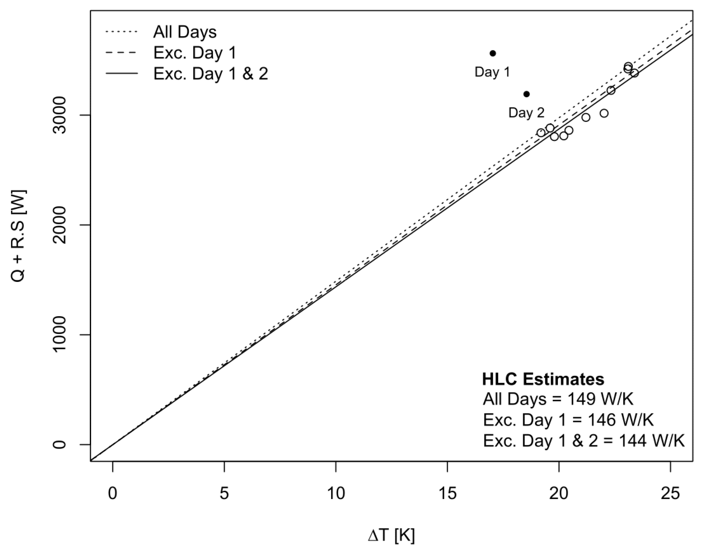
It is, however, crucial that suitable conditions are reached before analysis begins to avoid bias. Figure 4 plots the multiple linear regression corrected results for case A2. Days 1 and 2 can be identified as outliers but supporting evidence is required to justify their removal. Examining the internal temperature and heating load in Figure 5 can clearly justify the removal of day 1, but not day 2. Instead, the heat flux into the walls needs to be examined, here clearly demonstrating that day 2 also represents part of this warm up period. The definition and removal of this warm up period, and consideration of the thermal history of a test dwelling, are clearly subtle and may require further measurements, particularly of the heating behaviour of large heavyweight elements.
4. Simulated Co-Heating Tests
Performing simulated co-heating tests allows a wider range of dwellings to be tested under a wider range of external environmental conditions. Furthermore, the estimated or measured HTC can be directly compared to a true value from simulation inputs/outputs. This means the accuracy of the test at given monitoring durations can be assessed more directly than in field tests.
The value of the true heat loss (Htrue) can be derived from the model inputs, including the U-values (U—W/m2K) and areas (A—m2) of each element, Equation (5). Here, infiltration losses, varying between test periods with wind and stack pressures, need to be included separately. Derived from simulation outputs, the mean infiltration heat loss () is divided by the mean ΔT () across each simulation interval. Alternatively, Htrue can be calculated directly from the simulation outputs, summing the mean heat flows across all elements, including infiltration losses, and dividing by the mean ΔT (Equation (6)).
Simulations for the present paper have been performed within EnergyPlus and are based upon the method described in Section 2 and following the commonly used protocol described in Johnston et al. [21]. This includes:
- Internal temperature of 25 °C
- Vertical global solar radiation used in regression
- 24 hour aggregation (6 a.m.–6 a.m.)
- Multiple linear regression (no-intercept)
- Infiltration only (i.e., no ventilation)
The simulations themselves assume:
- Electrical heating with 100% efficiency
- Uniform internal temperatures
- Quasi steady state conditions achieved
- No local shading
- Zero party wall heat transfer
These simulations omit some experimental sources of uncertainty that may cause systematic bias (e.g., sensor measurement errors, party wall heat transfer). As seen previously, unsatisfactory results are likely to be achieved if such uncertainties exist. As such, these results represent tests conducted under ideal experimental conditions and should be assessed in reference to field tests previously discussed. As demonstrated within this paper, systematic errors such as party wall heat transfer, instrument calibration offsets, inhomogeneous internal temperatures and inappropriate solar measurements can lead to inaccurate results whatever the test duration.
4.1. Simulated Test Dwellings
For this paper, a range of simulated dwellings have been tested in order to expose the sensitivities of when and how long it takes for accurate HTC estimates to be achieved. These are designed to highlight indicative of trends amongst the broad UK housing stock, rather than provide an exhaustive array of tests. The simulated dwellings therefore cover a range of typical house types, built forms, constructions and levels of thermal performance, summarised in Figure 6.
Table 3 and Table 4 below. Thermal performance is based upon a typical UK Victorian dwelling [9] and upon current regulations for building regulation limits, notional [10] and Passivhaus dwellings [54]. All cases are then simulated across the Finningley IWEC2 weather file [55], representing typical UK weather conditions. Infiltration rates will vary across different test conditions, with mean air change rates due to infiltration during simulations listed in Table 3. Although the relationship between the two is not straightforward, these approximately correspond to those of typical a Victorian dwelling (16 m3/hm2 @50 Pa) and of UK regulatory levels for building regulation limits (10 m3/hm2 @50 Pa), notional (5 m3/hm2 @50 Pa) and Passivhaus dwellings (0.6 m3/hm2 @50 Pa).
4.2. Simulated Durations
To support and expand on the analysis of field test data, a series of simulated co-heating tests have been performed. Similar checks are made upon the time taken for results to converge to within 10%, of Htrue (Equation (5)). The time taken to achieve this level of accuracy is demonstrated for a number of dwelling types in the histograms in Figure 7. These figures show the results of simulations across a full year, with a new test period starting each day and running until a result is obtained to within the required accuracy of Htrue. These durations are then plotted and listed within each figure.
4.3. Required Duration and Construction Type
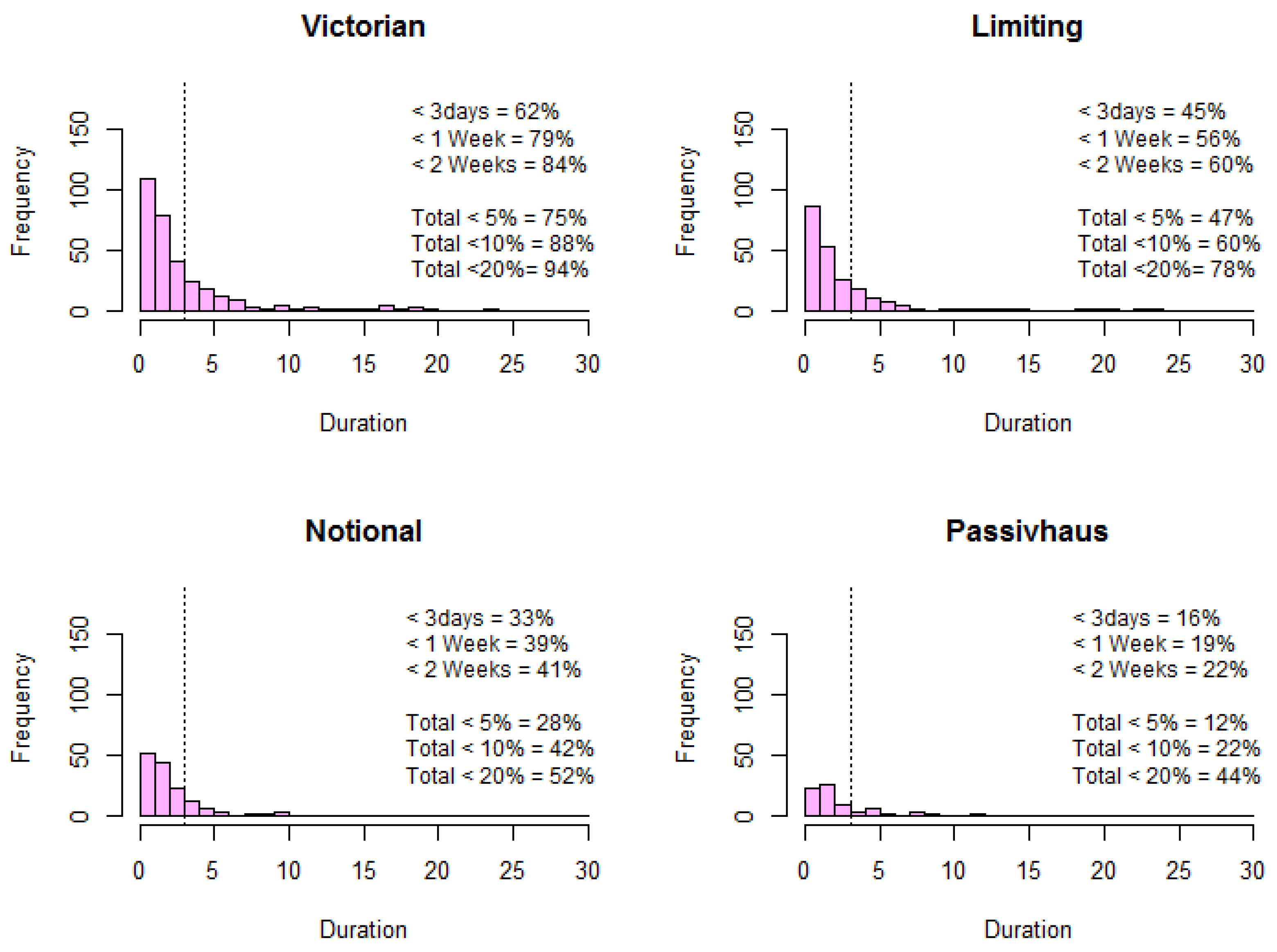
Figure 7 demonstrates two key points. Firstly, the conditions in which accurate measurements can be made reduces with increasing thermal performance. Measurements to within 10% of the true value can be obtained for large parts of the year for both Victorian (88% of year) and limiting (60%) test dwellings. The range of suitable conditions decreases significantly when moving towards the higher performance of a notional test dwelling (42%) and even more so in the Passivhaus case (22%). Interestingly, if the required accuracy is reduced from within 10% to within 20% of Htrue, the number of successful Passivhaus tests doubles (22 to 44%) whilst other dwelling types show more modest increases. This further indicates the difficultly in achieving accurate measurements in Passivhaus dwellings, particularly in avoiding underestimation due to components of stored solar heat [56]. This means that whilst there may be suitable periods for testing all dwellings, very high performance dwellings remain restricted and any tests performed run the risk of inaccurate results or failure.
The second point to note is that when results can be achieved, the majority of these will be within 72 h for all constructions—reinforcing the results seen within the field test analysis. Only modest increases in test periods are seen by extending the test period to one week or beyond.
4.4. Characteristics Determining Range of Suitable Test Conditions
In Figure 8, the required duration is shown across the same simulated year for the previous limiting and notional dwellings. It is clear the shortest results are achieved during cold, dull winter periods. In warmer, sunnier periods, uncertainty relating to solar gains increases, both absolutely and in relatively in proportion to other heat flows as ΔT decreases. Further, solar gains can disrupt the quasi steady state conditions set up by the test when gains exceed losses and temperatures peak. Valid results are not achieved in cases in which the internal temperature rises above the experimental set-point temperature (Ti > Tsetpoint) for extended periods (i.e., across a whole aggregation interval). At this point, dynamic heat flows dominate and the absence of significant electrical heating input means co-heating regression analysis significantly underestimates heat loss or become nonsensical. This means that test dwellings with low HTC (e.g., small exposed envelop areas, well-insulated) and high amounts of solar gains (e.g., highly glazed, south-orientation, little shading) are the most likely to experience solar driven systematic underestimate bias or to fail completely. Whilst this means most successful and shorter test periods are obtained in dull, cold periods across winter months, short successful periods may occur during warmer months when conditions are overcast and cool. In such cases, test periods must be short to avoid excessive solar radiation both before and during testing, meaning there is significant inherent risk in testing at such times.
It can then be noted that the likelihood of experimental overheating is reduced by increasing Tsetpoint, reducing any electrical baseload (non-thermostatically controlled equipment, e.g., mixing fans) or by applying additional shading to the test home. However, care must be taken to estimate the impact of any such changes upon the expected heat loss of the dwelling and the practicalities of their deployment.
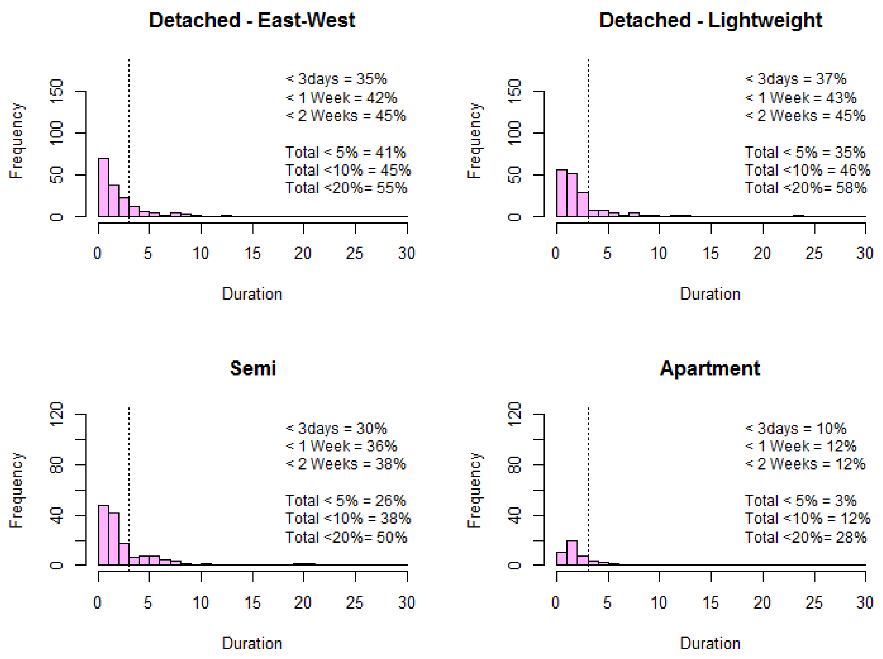
Figure 9 expands on this investigation, showing the changing distribution of results when the detached notional dwelling seen in Figure 7 is varied. Initially, the same notional construction is examined within two different built forms, a semi-detached dwelling and an apartment. Here, as the exposed envelope area reduces, the relative size of uncertainties increase and there is a higher propensity of the dwelling to overheat. Whilst the semi-detached dwelling provides accurate results over a slightly reduced period when compared to the larger detached dwelling (38% of the test year from 42%), apartments can only be successfully tested for restricted periods (12%). Further, any party wall heat transfer omitted from the simulations, is likely to further increase the risk of systematic bias and makes testing such dwellings challenging and prone to errors.
A further example changes the orientation of the detached notional dwelling onto an East–West, rather than North–South axis. The result is that solar gains are reduced along with any associated uncertainty, whilst the risk of unstable internal temperatures decreases, although the measurement of solar radiation for use in regression is more complex. The result is that an identical dwelling, orientated East–West instead of North–South, can be tested across a marginally wider range of conditions (45% compared to 42%).
Finally, the thermal mass of the notional dwelling is reduced (from a thermal mass parameter of 321 kJ/m2K to 112 kJ/m2K), creating a lightweight case. This construction maintains the same overall heat loss as the previous case, but replaces the previous construction with a brick clad timber frame, floating solid floor and plasterboard and timber internal walls. Here, with dynamic flows reduced, a marginal improvement in the range of test conditions can be seen (46% compared to 42%).
5. Discussion
The results of both the field tests and the simulated results indicate that in many cases co-heating tests can be performed in shorter time periods than previously suggested. In most cases (12 of 16), accurate results to within ±10% the value obtained from a full monitoring period can be achieved with 72 h of measurement—significantly short than the 1–4 week durations currently recommended. Importantly, there are only very modest gains achieved by extending the test period to one week or beyond. This result is supported by a number of simulated co-heating tests, performed across a range of built forms and constructions. Under suitable weather conditions and with sufficient experimental control and method, many tests will achieve the same result of a full test period within just 3 days, whilst the majority of achievable results occur within 7 days. This is significantly shorter than previously suggested and could significantly reduce the practical obstacles presently restricting the deployment of co-heating tests. However, convergence is no measure of an accurate result, such that experimental technique and an understanding of uncertainties remain crucial.
Among the field tests analysed, there are instances in which results do not satisfactorily converge—particularly under unsuitable experimental methods. This includes tests in which conditions are not constant throughout monitoring, such as variable party wall heat transfer. Additionally, cases in which solar radiation is measured horizontally may lead to significant jumps in HTC estimation throughout the monitoring period, along with systematic bias, as defined in Stamp [23,56]. Adopting the ISO 9869:2014 criteria from in-situ U-value measurements can help highlight such uncertainties. Plotting the estimated HTC as it evolves across a test period, as within this paper (Figure 1, Figure 2 and Figure 3), can also help highlight these experimental uncertainties and changing test conditions.
It is important to state these results in context. It should also be re-iterated that apparent convergence is not itself a guarantee of an accurate measurement. Shortening the length of co-heating tests can therefore not be done without increasing the risk of either inaccurate estimates or not achieving any estimate of the HTC. Further research on a wider number of dwellings is therefore required to re-enforce these findings. Further analysis should be conducted over a wider range of buildings and climates, including beyond the UK climate which has been the focus here.
Moving forward, focus must shift onto practicalities and the objectives of testing. If testing is to be conducted during post-construction, prior to occupation, it could be suggested that, ideally, testing could be conducted across a single weekend, during which most construction sites are shut down. If a house could be pre-heated whilst work access was maintained, then testing across a weekend or extended weekend may be feasible, certainly to a degree of accuracy that would diagnose dwellings with significant discrepancies that may warrant further investigation. On this final point it should be noted that tests to date have been reported to be 1.6 higher than predicted [7], meaning less stringent requirements for accuracy are likely to be required to identify significantly underperforming dwellings. After all, the co-heating HTC measurement only indicates the level of heat loss, not the underlying causes. From a research perspective, further multidisciplinary work under a broader scope is then required to reveal the underlying processes. In terms of quality assurance, a larger sample of less accurate tests is likely to be more useful to demine the extent of underperformance and highlight cases and trends of significant underperformance.
At shorter test lengths, practicalities become increasingly important. The total duration for testing becomes is not only affected by any warm up period but also by the setting up and dismantling of equipment. The total cost of testing a reflection of not only test lengths but the cost of equipment, complexity of analysis and skill of tester. Practically, many new buildings will have excess moisture levels associated with construction during the small window for testing post-construction and pre-occupation. This will either increase the required testing time or add significant uncertainty to HTC estimates. Therefore, whilst the durations for co-heating tests reported within this paper have moved closer to those of short term dynamic tests, in both cases, practical issues remain equally important, particularly if testing is to be done at any scale. The relative simplicity of the co-heating test must be weighed up against the additional information gathered by dynamic methods and their respective strengths.
Finally, the range of suitable testing conditions varies significantly based on the built form, construction type and typical weather conditions expected for a test dwelling. Whilst this leaves a reasonably long testing season for high heat loss, large dwellings (greater than 60% of a year for the example dwelling built to current building regulation limits or less), this is reduced to 38%–46% of the year for same building built to notional standards.
Very low heat loss, highly glazed, heavyweight dwellings or those with small overall exposed areas can then expect to deliver reliable results for even more restricted periods (Passivhaus ~22%, apartments ~12%) and not without significant risks of failure. Whilst such dwellings have been successfully tested [57], they carry higher inherent risk and increased relative uncertainties—particularly from unstable internal temperatures and underestimated HTCs due to stored solar components [56]. Whilst this could mean extended testing durations are required (e.g., 6–8 weeks [37]), longer tests are unlikely to reduce any bias and shorter, highly selective periods are likely to yield improved results. Further analysis of field test results for such dwellings is needed. Nevertheless, it is unlikely such dwellings can be tested to high accuracies or at any significant scale and alternative approaches may be required, including the deployment of external shading to reduce solar gains during testing or alternative experimental procedures. The type of simulated tests performed in this paper could be used to predict when a test could be performed and assess the risk prior to testing.
6. Conclusions
In 12 of 16 field tests, co-heating HTC measurements have been shown to converge to within ±10% of their value obtained over a full test period within just 72 h—significantly shorter than typical test durations. Only small improvements in accuracy of reliability are achieved by monitoring beyond this point, whilst many systematic errors will not be reduced. These results are supported by simulated tests across a wider range of buildings and environmental conditions. In non-convergent cases, significant experimental uncertainties can be cited—highlighted by plotting HTC estimates a function of test duration and through application of ISO 9869:2014 in situ U-value criteria. It is recommended such details are reported for all tests, to both further establish the relationship between test length and accuracy across a wider range of buildings and to examine potential uncertainties in individual tests. Finally, the range of suitable test conditions varies significantly with construction, built form and solar characteristics. Example dwellings built to 2012 UK building regulation limits may be tested for around two-thirds of a year. However, this reduces to around 40% of the year for the same example dwelling built to notional requirements and to just 20% in Passivhaus or 12% in apartments. Clearly these latter cases cannot be conducted without a degree of risk and alternative or modified methods are likely to be required.
Acknowledgments
This research was made possible by support from the EP-SRC Centre for Doctoral Training in Energy Demand (LoLo), grant numbers EP/L01517X/1 and EP/H009612/1. For secondary data used within the analysis, the authors are grateful to the NHBC and participants of the NHBC co-heating field trial: BRE, BSRIA, STROMA, Cardiff University—Welsh School of Architecture, Loughborough University, Nottingham University and also to Leeds Beckett University.
Author Contributions
Experiments, simulations and data analysis have been conducted by Samuel Stamp with guidance and support from Robert Lowe and Hector Altamirano-Medina.
Conflicts of Interest
The authors declare no conflict of interest.
References
- Doran, S. Field Investigations of the Thermal Performance of Construction Elements as Built; Building Research Establishment: Watford, UK, 2000. [Google Scholar]
- Baker, P.H. Technical Paper 10: U-Values and Traditional Buildings-In Situ Measurements and Their Comparisons to Calculated Values; Historic Scotland, Glasgow Caledonian University: Glasgow, UK, 2011. [Google Scholar]
- Rye, C. The SPAB Research Report 1: U-Value Report; Society for the Protection Ancient buildings: London, UK, 2011. [Google Scholar]
- Cesaratto, P.G.; De Carli, M.; Marinetti, S. Effect of different parameters on the in situ thermal conductance evaluation. Energy Build. 2011, 43, 1792–1801. [Google Scholar] [CrossRef]
- Adhikari, R.S.; Lucchi, E.; Pracchi, V. Experimental measurements on thermal transmittance of the opaque vertical walls in the historical buildings. In Proceedings of the PLEA2012—28th Conference, Opportunities, Limits & Needs towards an Environmentally Responsible Architecture, At Lima, Peru, 7–9 November 2012. [Google Scholar]
- Li, F.G.N.; Smith, A.Z.P.; Biddulph, P.; Hamilton, I.G.; Lowe, R.; Mavrogianni, A.; Oikonomou, E.; Raslan, R.; Stamp, S.; Stone, A.; et al. Solid-wall U-values: Heat flux measurements compared with standard assumptions. Build. Res. Inf. 2015, 43, 238–252. [Google Scholar] [CrossRef]
- Johnston, D.; Miles-Shenton, D.; Farmer, D. Quantifying the domestic building fabric ‘performance gap’. Build. Serv. Eng. Res. Technol. 2015, 36, 614–627. [Google Scholar] [CrossRef]
- Lowe, R.J.; Wingfield, J.; Bell, M.; Bell, J.M. Evidence for heat losses via party wall cavities in masonry construction. Build. Serv. Eng. Res. Technol. 2007, 28, 161–181. [Google Scholar] [CrossRef]
- Building Research Establishment (BRE). The UK Governments Standard Assessment Procedure (SAP); BRE: Garston, UK, 2013. [Google Scholar]
- Department for Communities and Local Government (DCLG). Conservation of Fuel and Power: Approved Document L1a; DCLG: London, UK, 2013.
- Lecompte, J. The influence of natural convection on the thermal quality of insulated cavity construction. Build. Res. Pract. 1990, 6, 349–354. [Google Scholar]
- Hens, H.; Janssens, A.; Depraetere, W.; Carmeliet, J.; Lecompte, J. Brick Cavity Walls: A Performance Analysis Based on Measurements and Simulations. J. Build. Phys. 2007, 31, 95–124. [Google Scholar] [CrossRef]
- Bankvall, C. Practical thermal conductivity in an insulated structure under the influence from workmanship and wind. In Proceedings of the ASTM symposium on Advances in Heat Transmission Measurement on Thermal Insulation Material Systems, Philadelphia, PA, USA, 19–20 September 1977. [Google Scholar]
- Zero Carbon Hub (ZCH). Closing the Gap between Design & As-Built Performance—Evidence Review Report; ZCH: Birmingham, UK, 2014. [Google Scholar]
- International Organization for Standardization (ISO). BS EN 1946-4:2000—Measurements by Hot Box Methods; International Organization for Standardization (ISO): Geneva, Switzerland, 2000. [Google Scholar]
- Carrié, R.; Kapsalaki, M.; Wouters, P. Right and Tight: What’s new in Ductwork and Building Airtightness? In Proceedings of the 34th AIVC—3rd TightVent—2nd Cool Roof Conference—1st Venticool Conference, Athens, Greece, 25–26 September 2013. [Google Scholar]
- ISO 9869-1:2014—Thermal Insulation—Building Elements—In-Situ Measurement of Thermal Resistance and thermal Transmittance—Part. 1: Heat Flow Meter Method; International Organization for Standardization (ISO): Geneva, Switzerland, 2014.
- International Organization for Standardization (ISO). BS EN ISO 13790:2008 Energy Performance of Buildings. Calculation of Energy Use for Space Heating and Cooling; ISO: Geneva, Switzerland, 2008. [Google Scholar]
- Baker, P.H. A Retrofit of a Victorian Terrace House in New Bolsover: A Whole House Thermal Performance Assessment; Historic England & Glasgow Caledonian University: Glasgow, UK, 2015. [Google Scholar]
- Wingfield, J. In Situ Measurement of Whole House Heat Loss Using Electric Coheating; Leeds Metropolitan University: Leeds, UK, 2010. [Google Scholar]
- Johnston, D.; Miles-Shenton, D.; Farmer, D.; Wingfield, J. Whole House Heat Loss Test Method (Coheating); Leeds Metropolitan University: Leeds, UK, 2013. [Google Scholar]
- Bauwens, G.; Roels, S. Co-heating test: A state-of-the-art. Energy Build. 2014, 82, 163–172. [Google Scholar] [CrossRef]
- Stamp, S.F. Assessing Uncertainty in Co-Heating Tests: Calibrating a Whole Building Steady State Heat Loss Measurement Method. Ph.D. Thesis, UCL (University College London), London, UK, 2016. [Google Scholar]
- Butler, D.; Dengel, A. NHBC Review of Co-Heating Test Methodologies; National House Building Council Foundation (NHBC): Milton Keynes, UK, 2013. [Google Scholar]
- Bell, M.; Lowe, R.J. The York Energy Demonstration Project—Final Report; Leeds Metropolitan University: Leeds, UK, 1998. [Google Scholar]
- Bell, M.; Wingfield, J.; Miles-Shenton, D.; Seavers, J. Low Carbon Housing—Lessons from Elm Tree Mews; Leeds Metropolitan University and Joseph Rowntree Foundation: Leeds, UK, 2010. [Google Scholar]
- Wingfield, J.; Bell, M.; Miles-Shenton, D.; Seavers, J. Elm Tree Mews Field Trial—Evaluation and Monitoring of Dwellings Performance—Final Technical Report; Leeds Metropolitan University: Leeds, UK, 2011. [Google Scholar]
- Miles-Shenton, D.; Wingfield, J.; Sutton, R.; Bell, M. Temple Avenue Project—Summary Report; Leeds Metropolitan University: Leeds, UK, 2011. [Google Scholar]
- Good Homes Alliance (GHA). GHA Monitoring Programme. 2009–2011: Technical Report—Results from Phase 1: Post-Construction Testing of a Sample of Highly Sustainable New Homes; Good Homes Alliance: London, UK, 2011. [Google Scholar]
- Palmer, J.; Godoy-Shimizu, D.; Tillson, A.; Mawditt, I. Bulding. Performance Evaluation Programme: Findings from Domestic Projects—Making Reality Match Design; Innovate UK: Swindon, UK, 2016.
- Latif, E.; Lawrence, M.; Shea, A.; Walker, P. In situ assessment of the fabric and energy performance of five conventional and non-conventional wall systems using comparative coheating tests. Build. Environ. 2016, 109, 68–81. [Google Scholar] [CrossRef]
- Johnston, D.; Farmer, D.; Miles-Shenton, D. Quantifying the aggregate thermal performance of UK holiday homes. Build. Serv. Eng. Res. Technol. 2017, 38, 209–225. [Google Scholar] [CrossRef]
- Farmer, D.; Gorse, C.; Swan, W.; Fitton, R.; Brooke-Peat, M.; Miles-Shenton, D.; Johnston, D. Measuring thermal performance in steady-state conditions at each stage of a full fabric retrofit to a solid wall dwelling. Energy Build. 2017. [Google Scholar] [CrossRef]
- Department of Communities and Local Government (DCLG). 2012 Consultation on Changes to the Building Regulations in England—Section Two—Part. L (Conservation of Fuel and Power); DCLG: London, UK, 2012.
- Everett, R. Rapid Thermal Calibration of Houses; Open University Energy Research Group: Milton Keynes, UK, 1985. [Google Scholar]
- Lowe, R.J.; Gibbons, C.J. Passive solar houses: Availability of weather suitable for calibration in the UK. Build. Serv. Eng. Res. Technol. 1988, 9, 127–132. [Google Scholar] [CrossRef]
- Alexander, D.K.; Jenkins, H.G. The Validity and Reliability of Co-heating Tests Made on Highly Insulated Dwellings. Energy Procedia 2015, 78, 1732–1737. [Google Scholar] [CrossRef]
- Baker, P.H.; van Dijk, H.A.L. PASLINK and dynamic outdoor testing of building components. Build. Environ. 2008, 43, 143–151. [Google Scholar] [CrossRef]
- Judkoff, R.; Balcomb, J.; Hancock, C.; Barker, G.; Subbarao, K. Side-by-Side Thermal Tests of Modular Offices: A Validatioin Study of the STEM Method; National Renewable Energy Laboratory: Golden, CO, USA, 2000.
- Sonderegger, R.C.; Modera, M.P. Electric co-heating: A method for evaluating seasonal heating efficiencies and heat loss rates in dwellings. In Proceedings of the Second International CIB Symposium, Copenhagen, Demark, 28 May–1 June 1979. [Google Scholar]
- Sonderegger, R.C.; Condon, P.E.; Modera, M.P. In-Situ Measurement of Residential Energy Performance Using Electric Coheating. In Proceedings of the American Society of Heating Refrigerating and Air Conditioning Engineers Semi-Annual Meeting Transactions, Los Angeles, CA, USA, 3 February 1980; Volume 86, p. 394. [Google Scholar]
- Subbarao, K. Primary and Secondary Terms-Analysis and Renormalization: A Unified Approach to Building and Energy Simulations and Short-Term Testing—A Summary; Solar Energy Research Institute: Colorado, CO, USA, 1988. [Google Scholar]
- Mangematin, E.; Pandraud, G.; Roux, D. Quick measurements of energy efficiency of buildings. C. R. Phys. 2012, 13, 383–390. [Google Scholar] [CrossRef]
- Pandruad, G.; Fitton, R. QUB: Validation of a rapid energy diagnosis method for buildings. In Proceedings of the Characterisation Based on Full Scale Dynamic Measurements 4th Expert Meeting, Holenkirchen, Germany, 8–10 April 2013. [Google Scholar]
- Andrews, J.W. Electric Coheating as a Means to Test Duct Efficiency: A Review and Analysis of the Literature; Brookhaven National Laboratory: New York, NY, USA, 1995.
- Liu, M.; Claridge, D.E. Improving Building Energy Performance through Continuous Commissioning; Energy Systems Laboratory, Texas A & M.: College Station, TX, USA, 1995. [Google Scholar]
- Roels, S.; Bacher, P.; Bauwens, G.; Madsen, H.; Jiménez, M.J. Characterising the Actual Thermal Performance of Buildings: Current Results of Common Exercises Performed in the Framework of the IEA EBC Annex 58-Project. Energy Procedia 2015, 78, 3282–3287. [Google Scholar] [CrossRef] [Green Version]
- Roels, S.; Bacher, P.; Bauwens, G.; Castaño, S.; Jiménez, M.J.; Madsen, H. On site characterisation of the overall heat loss coefficient: Comparison of different assessment methods by a blind validation exercise on a round robin test box. Energy Build. 2017, 153, 179–189. [Google Scholar] [CrossRef]
- Farmer, D.; Johnston, D.; Miles-Shenton, D. Obtaining the heat loss coefficient of a dwelling using its heating system (integrated coheating). Energy Build. 2016, 117, 1–10. [Google Scholar] [CrossRef]
- Jack, R. Building Diagnostics: Practical Measurement of the Fabric Thermal Performance of Houses. Ph.D. Thesis, Loughborough University, Loughborough, UK, 2015. [Google Scholar]
- Jack, R.; Loveday, D.; Allinson, D.; Lomas, K. First evidence for the reliability of building co-heating tests. Build. Res. Inf. 2017, 1–19. [Google Scholar] [CrossRef]
- Joint Committee for Guides in Metrology (JCGM). JCGM 100:2008—Evaluation of Measurement Data—Guide to the Expression of Uncertainty in Measurement; JCGM: Paris, France, 2008. [Google Scholar]
- PD 6461-4:2004—General Metrology. Practical Guide to Measurement Uncertainty. Available online: https://shop.bsigroup.com/ProductDetail/?pid=000000000030044787 (accessed on 3 October 2017).
- Feist, W. Passive House Planning Package; Passivhaus Institut: Darmstadt, Germany, 2007. [Google Scholar]
- EnergyPlus Weather Data by Location. Available online: https://energyplus.net/weather-location/europe_wmo_region_6/GBR/GBR_Finningley.033600_IWEC (accessed on 15 November 2016).
- Stamp, S.; Altamirano-Medina, H.; Lowe, R. Measuring and accounting for solar gains in steady state whole building heat loss measurements. Energy Build. 2017, 153, 168–178. [Google Scholar] [CrossRef]
- Johnston, D.; Siddall, M. The Building Fabric Thermal Performance of Passivhaus Dwellings—Does It Do What It Says on the Tin? Sustainability 2016, 8. [Google Scholar] [CrossRef]
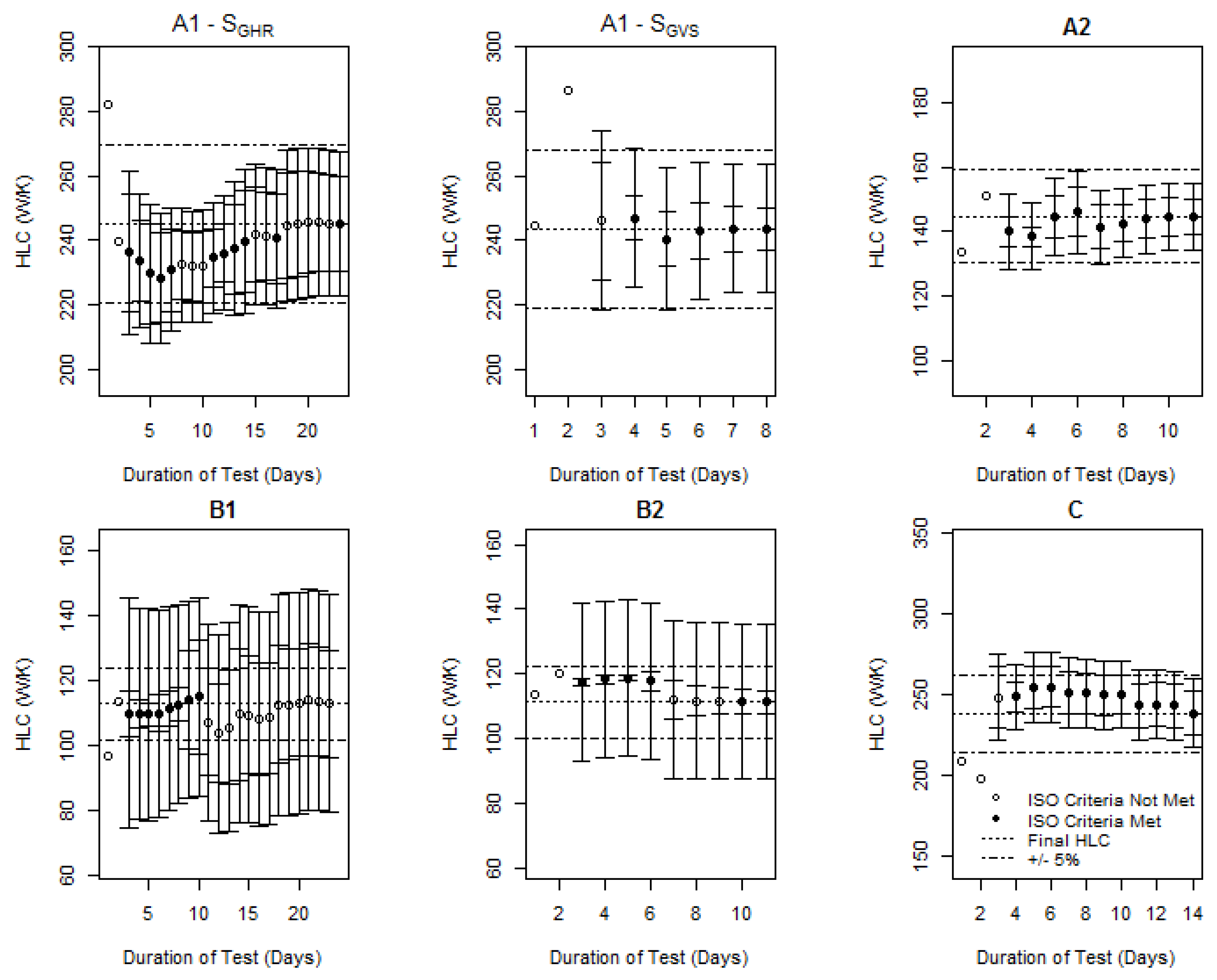
Figure 1.
Estimated heat transfer coefficient (HTC) across the full test duration for six field tests. Case A1 includes analysis with both a south-facing vertical solar measurement (SGVS) and a global horizontal measurement (SGHR). Case B1 uses SGHR whilst all other cases use a single vertical measurement. Cases A1 and A2, feature one guarded wall. Cases B1 and B2 feature one guarded and one unguarded wall, whilst C a large detached dwelling.

Figure 2.
Estimated HTC across the full test duration for a further six field tests. Case I is a corner apartment with some unguarded adjoining spaces. Case E and F use a horizontal solar radiation measurement.
Figure 2.
Estimated HTC across the full test duration for a further six field tests. Case I is a corner apartment with some unguarded adjoining spaces. Case E and F use a horizontal solar radiation measurement.
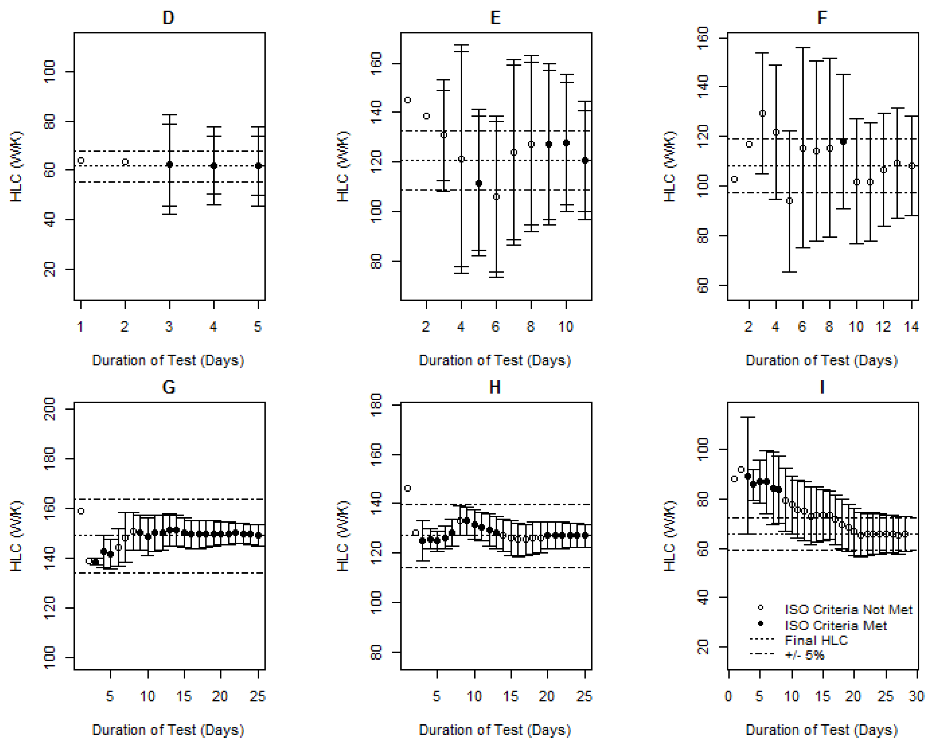
Figure 3.
Estimated HTC across the full test duration for a further five field tests, performed by different organisations on the same test dwelling. Cases J1 and J4 use a horizontal measurement of solar radiation.
Figure 3.
Estimated HTC across the full test duration for a further five field tests, performed by different organisations on the same test dwelling. Cases J1 and J4 use a horizontal measurement of solar radiation.
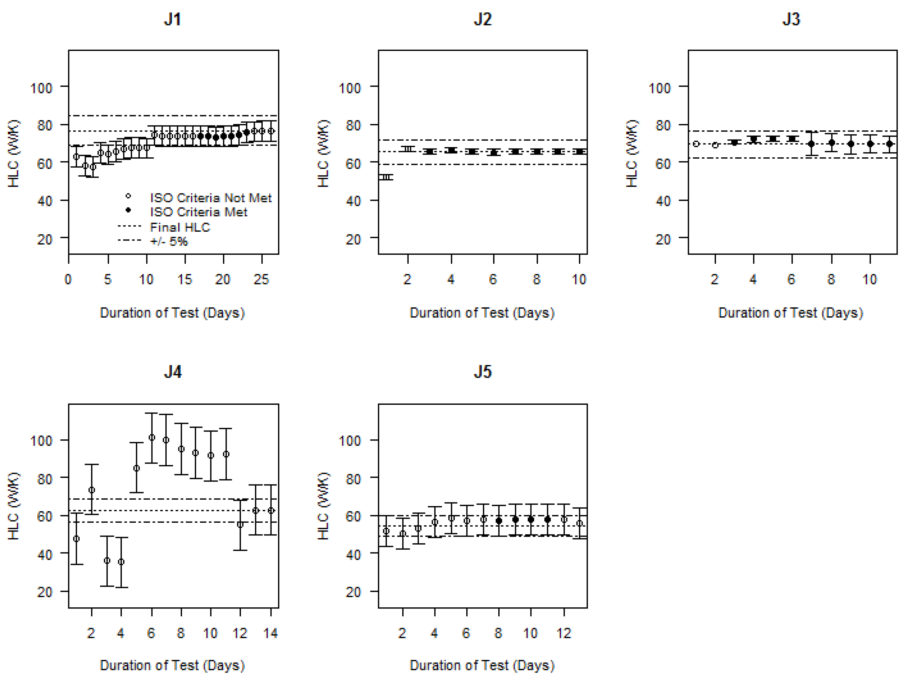
Figure 4.
Solar corrected, multiple linear regression (MLR) plot for field test (Case A2) with two biased data points. Results for all data points are compared to those excluding days 1 and excluding day 1 and 2 in the figure.
Figure 4.
Solar corrected, multiple linear regression (MLR) plot for field test (Case A2) with two biased data points. Results for all data points are compared to those excluding days 1 and excluding day 1 and 2 in the figure.

Figure 5.
Corresponding (A) average interal temperature, (B) electric heating power, Qelec, and (C) heat flux measurements.
Figure 5.
Corresponding (A) average interal temperature, (B) electric heating power, Qelec, and (C) heat flux measurements.
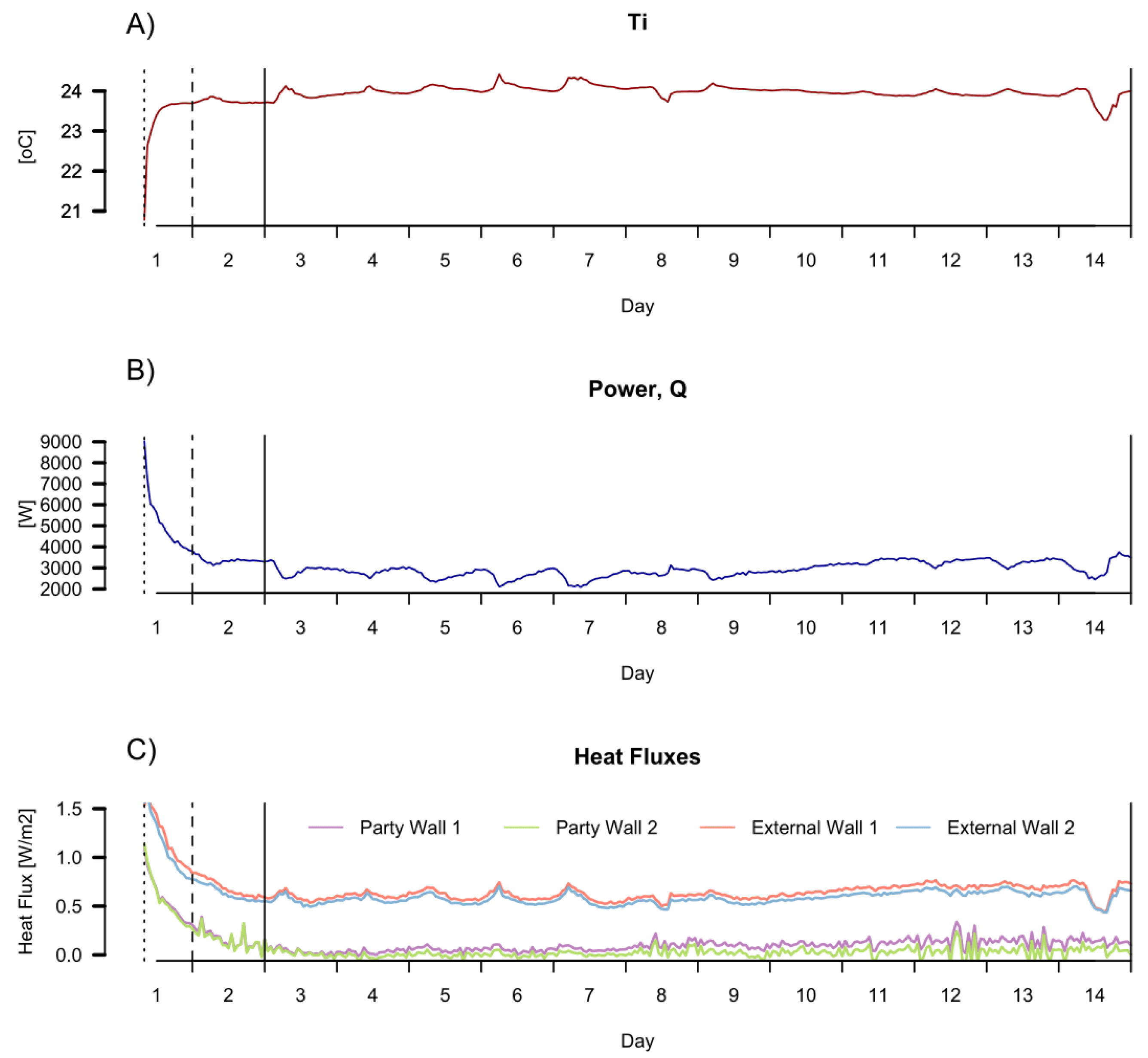
Figure 6.
Built form of simulated test dwellings.
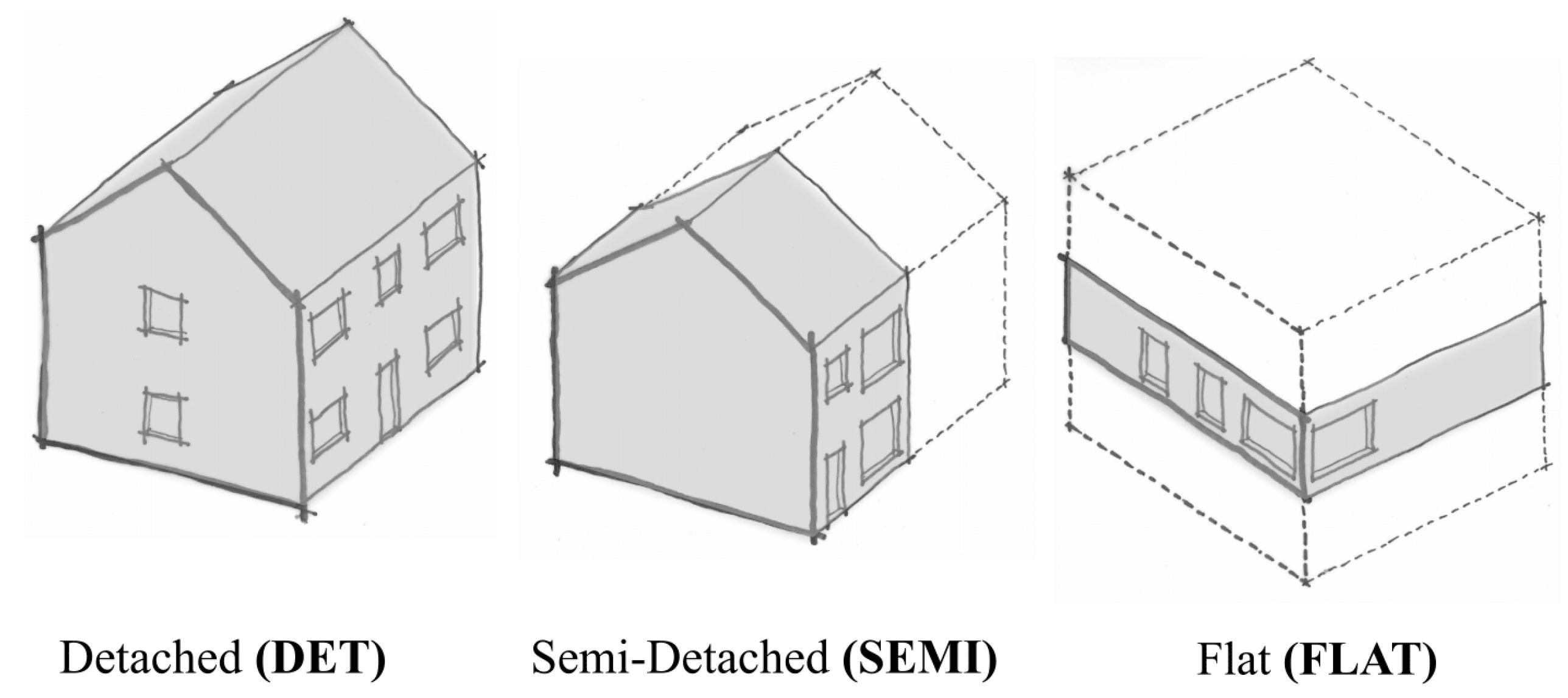
Figure 7.
Distribution of required test duration in a detached simulated dwelling of various constructions. Mean Htrue across this period are: Victorian = 625 W/K, Limiting = 215 W/K, Notional = 110 W/K, Passivhaus = 68 W/K. The proportion of the year in which results converge to within 5%, 10% and 20% are included in each plot, alongside the percentage of results achieved within 3 days, 1 and 2 weeks.

Figure 8.
Required test duration across simulated weather file for limiting and notional dwellings. Gaps in the data indicate periods in which a result to within 10% of true value was never achieved.
Figure 8.
Required test duration across simulated weather file for limiting and notional dwellings. Gaps in the data indicate periods in which a result to within 10% of true value was never achieved.
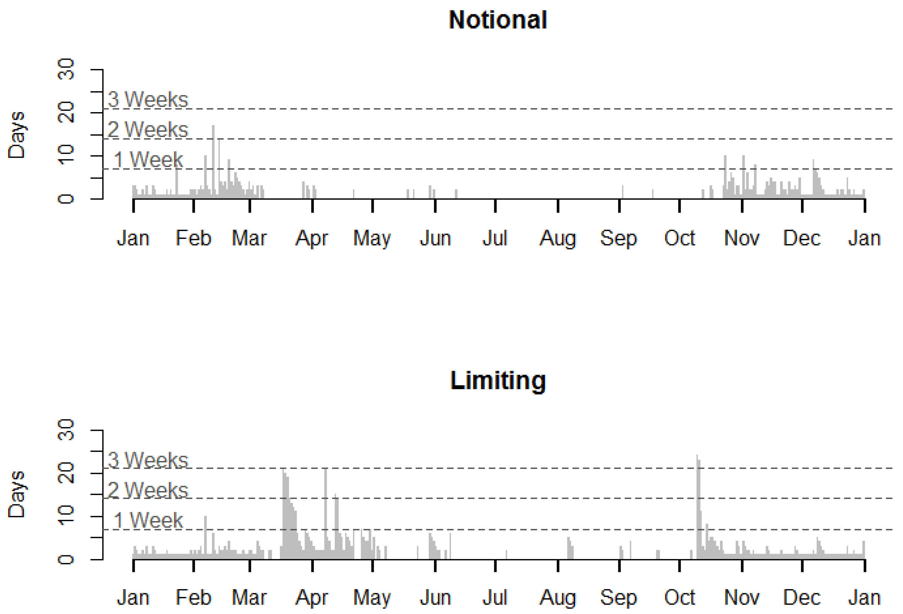
Figure 9.
Distribution of required test duration in four simulated dwellings. Mean Htrue across this period are: Notional Lightweight and East–West = 110 W/K, Semi = 68 W/K, Apartment = 31 W/K.
Figure 9.
Distribution of required test duration in four simulated dwellings. Mean Htrue across this period are: Notional Lightweight and East–West = 110 W/K, Semi = 68 W/K, Apartment = 31 W/K.


Table 1.
Summary details of field tests and test dwellings. Error estimates (stated at 95% confidence intervals) for primary cases are calculated based upon the method set out in Stamp [23], incorporating both measurement errors and statistical errors. Due to a lack of full details, secondary cases are based upon the standard error of regression alone, therefore representing a smaller range.
| Case | When | Hmeas (W/K) | Hpred (W/K) | Construction | Type | Notes |
|---|---|---|---|---|---|---|
| Primary Cases | ||||||
| A1 | January–February | 243 ± 10 | 212 | Brick-cavity-block (un-insulated) | Semi | One guarded adjoining property (Case B1). Both horizontal and vertical solar measurements taken. |
| A2 | March–April | 144 ± 10 | 112 | Brick-cavity-block (insulated) | Semi | Same dwelling as above, after cavity walls insulated. |
| B1 | March–April | 113 ± 33 | 105 | Brick-cavity-block (insulated) | Mid-terrace | One party wall guarded, one unguarded. |
| B2 | January–February | 111 ± 24 | 105 | Brick-cavity-block (insulated) | Mid-terrace | One party wall unguarded, one unguarded. Repeated test of case B1. |
| C | March | 238 ± 21 | 205 | Masonry thin-joint | Detached | Large detached |
| D | December | 62 ± 16 | 66 | Timber frame with lower concrete retaining walls | Detached | Passivhaus dwelling. |
| E | December | 121 ± 23 | 78 | Aerated blocks | Detached | Horizontal solar radiation measured. |
| Secondary Cases | ||||||
| F | February | 108 ± 20 | 94 | Aerated blocks | Semi | Horizontal solar radiation measured. Unguarded neighbouring property. |
| G | January–February | 149 ± 8 | 129 | Masonry thin-joint | Detached | [28] |
| H | January–February | 127 ± 5 | 120 | Structurally insulated panel | Detached | [28] |
| I | March–April | 66 ± 7 | 38 | Clay-block in concrete frame | Corner apartment | Guarded and unguarded surrounding apartments. |
| J1–J5 | February | 56–76 | 68 | Brick clad timber frame | Detached | Detached dwelling, tested by various organisations between December–April [24] |
Table 2.
Required duration for field tests. Instances in which convergence criteria are only temporarily met are indicated by an asterisk *. The days to reach ISO criteria only includes occasions in which these criteria are held true for the remainder of the test period.
Table 2.
Required duration for field tests. Instances in which convergence criteria are only temporarily met are indicated by an asterisk *. The days to reach ISO criteria only includes occasions in which these criteria are held true for the remainder of the test period.
| Test Case | Days <20% | Days <10% | Days <5% | Days to ISO | Monitoring Durations | Warm Up Period |
|---|---|---|---|---|---|---|
| A1 (SGHR) | 1 | 2 | 2–4 *, 11 | - | 24 | 5 |
| A1 (SGVS) | 1 | 3 | 3 | 4 | 8 | 5 |
| A2 | 1 | 1 | 2 | 3 | 11 | 2 |
| B1 | 1 | 2 | 2 | - | 24 | 5 |
| B2 | 1 | 1 *, 3 | 1 *, 7 | 10 | 11 | 2 |
| C | 1 *,3 | 3 | 3 | 3 | 14 | 4 |
| D | 2 | 2 | 3 | 3 | 5 | 1 |
| E | 1 | 1 | 1*,3 | 9 | 13 | 5 |
| F | 1 | 5 | 12 | - | 14 | - |
| G | 1 | 2 | 2 | 9 | 25 | - |
| H | 1 | 1 | 2 | 20 | 25 | - |
| I | 10 | 17 | 19 | - | 29 | - |
| J1 | 1 *, 4 | 11 | 11 | - | 28 | - |
| J2 | 2 | 2 | 2 | 3 | 10 | - |
| J3 | 1 | 1 | 1 | 3 | 11 | 1 |
| J4 | 2 *, 12 | 13 | 13 | - | 14 | - |
| J5 | 1 | 1 | 3 | - | 13 | - |
Table 3.
Summary details of simulated test dwellings.
| Built Form | Detached | Semi | Apartment |
|---|---|---|---|
| Floor Area (footprint) | 58.1 m2 | 38 m2 | 67 m2 |
| Total Floor Area | 116.3 m2 | 76 m2 | 67 m2 |
| Volume | 348.9 m3 | 190.1 m3 | 167.5 m3 |
| Envelope area (exc. Ground floor) | 242.0 m2 | 127.3 m2 | 55 m2 |
| Party wall/floor area | - | 35 m2 | 190.3 m2 |
| Glazed area | 21.3 m2 | 16.1 m2 | 14.7 m2 |
| Glazing fraction | 18.3% | 21.2% | 21.9% |
Table 4.
Construction details and U-values of elements used within simulated dwellings.
| Construction | Walls | Ground Floor | Glazing | Roof | Mean ACH | Partition Walls | Internal Floors |
|---|---|---|---|---|---|---|---|
| Victorian | 220 mm Solid Brick walls (2.1 W/m2K) | Uninsulated suspended timber floor (0.8 W/m2K) | Single glazing (4.8 W/m2K, g = 0.85) | Pitched roof, uninsulated (2.3 W/m2K) | 0.82 h−1 | 110 mm solid brick, plaster | Timber, plaster on lathe |
| Modern dwellings | Full fill brick and aircrete block | Insulated concrete floor | Double glazing (1.4 W/m2K, g = 0.63) | Pitched roof—insulated at ceiling level | - | 12 mm plaster-lightweight block-12 mm plaster | Timber, plasterboard |
| Limiting | 0.30 W/m2K | 0.25 W/m2K | 2.0 W/m2K g = 0.76 | 0.20 W/m2K | 0.57 h−1 | - | - |
| Notional | 0.18 W/m2K | 0.13 W/m2K | 1.4 W/m2K g = 0.63 | 0.13 W/m2K | 0.23 h−1 | - | - |
| Passivhaus | 0.15 W/m2K | 0.15 W/m2K | 0.85 W/m2K g = 0.5 | 0.15 W/m2K | 0.03 h−1 | - | - |
© 2017 by the authors. Licensee MDPI, Basel, Switzerland. This article is an open access article distributed under the terms and conditions of the Creative Commons Attribution (CC BY) license (http://creativecommons.org/licenses/by/4.0/).
Share and Cite
MDPI and ACS Style
Stamp, S.; Altamirano-Medina, H.; Lowe, R. Assessing the Relationship between Measurement Length and Accuracy within Steady State Co-Heating Tests. Buildings 2017, 7, 98. https://doi.org/10.3390/buildings7040098
AMA Style
Stamp S, Altamirano-Medina H, Lowe R. Assessing the Relationship between Measurement Length and Accuracy within Steady State Co-Heating Tests. Buildings. 2017; 7(4):98. https://doi.org/10.3390/buildings7040098
Chicago/Turabian StyleStamp, Samuel, Hector Altamirano-Medina, and Robert Lowe. 2017. "Assessing the Relationship between Measurement Length and Accuracy within Steady State Co-Heating Tests" Buildings 7, no. 4: 98. https://doi.org/10.3390/buildings7040098
Note that from the first issue of 2016, this journal uses article numbers instead of page numbers. See further details here.