Optimized Operation of an Existing Public Building Chilled Station Using TRNSYS

1
School of Architecture, Dalian University of Technology, Dalian 116024, China
2
Department of Construction Engineering, Dalian University of Technology, Dalian 116024, China
3
School of Architecture and Interior Design, University of Cincinnati, OH 45221, USA
4
Department of Civil and Architectural Engineering and Construction Management, University of Cincinnati, OH 45221, USA
*
Author to whom correspondence should be addressed.
Buildings 2018, 8(7), 87; https://doi.org/10.3390/buildings8070087
Submission received: 10 May 2018
/
Revised: 21 June 2018
/
Accepted: 2 July 2018
/
Published: 3 July 2018
Abstract
:Taking an existing public building as an example, the mathematical model of each equipment module of the chilled station and the TRNSYS custom module are established on the basis of the measured data. The mathematical model of “chilled station cooling capacity—equipment power” is proposed and established. The full-frequency control strategy based on device contribution rate is proposed. The TRNSYS simulation platform is used to simulate a public building chilled station in the cooling season. The result shows that the seasonal energy efficiency rate of the public building air-conditioning system is 2.15 times as high as the original after applying the new control strategy.
1. Introduction
Thirty-two public buildings in China have been carefully investigated and the investigation results show that the current chilled station equipment of air conditioning system is mostly controlled by changing the number of operating devices manually, while the air conditioning terminal remains unchanged and the automatic control system is actually in a paralyzed state. Moreover, the air conditioning system has problem of low energy efficiency in a handful of public buildings even though their automatic control system works. This research focuses on improving the situation.
Some research shows that, the chillers will save 9.5% energy after the chiller unit is frequency-converted throughout the year. Pumps and cooling tower fans will be transformed into fully variable frequency fans, and with optimized control logic, the cold station system will save 24% of energy throughout the year, and system energy efficiency will increase significantly [1,2]. Single device’s energy saving is not necessarily equivalent to high energy efficiency of the system due to the full conversion of chilled station can significantly increase the energy efficiency of the system [3,4]. Chilled station full frequency conversion can minimize the air conditioning energy consumption [5]. Combining chilled water, cooling water and a direct digital control (DDC) system’s integrated machine room group control system, which can increase human comfort and energy utilization efficiency [6,7,8]. Chilled station automatic control system can significantly improve the energy-saving effect, the operation is more convenient and accurate. At present, the chilled station operation control method mainly uses variable flow control and variable water temperature control [9,10,11,12]. Many scholars have simulated the energy consumption of air-conditioning systems and results show that TRNSYS software has high accuracy [13,14]. TRNSYS software can be applied to calibrate experimental data and simulate energy of the air conditioning system, thereby optimizing control strategy [15,16,17].
Scholars have done some research in order to improve the energy efficiency of the chilled station, currently focusing on variable flow control and variable water temperature control, which is lack of chilled station full frequency conversion with equipment frequency control strategy. The automatic control system of a public building was regarded as the object of study, the optimal control strategy for chilled station was studied thoroughly in this paper using TRNSYS software. However, the terminal regulation of the air conditioning system was not considered in this study.
2. Research Context
2.1. Basic Information
An existing public building (hereinafter referred to as the test building) in Dalian of China was studied in this paper. Its nameplate parameters of the equipment in air conditioning system are shown in Table 1. It is equipped with a direct digital control system (DDC system) and automatic control system of air conditioners, with an airflow bypass valve provided between the inlet and outlet ducts. The water supply amount was adjusted in order to satisfy cold load variation according to the temperature difference of the supply and return water. The cooling-dominated season was from 1 July to 30 September, with a total of 92 days, and the operation duration was from 8:30 to 17:30, i.e., 9 h/day.
In Table 1, Qch represents the chiller rated cooling capacity, N represents rated power, G represents rated flow and H represents rated head, r represents rotating speed.
400 sets of operation data were selected in order to analyze and calculate the operating characteristics of the test building chilled station.
2.2. Operating Characteristics
The operation of air conditioning system is characterized by the energy efficiency of a single device and the system. The two operating characteristic parameters, the chiller’s energy efficiency ratio and the Seasonal Energy Efficiency Rate of air conditioning engineering (SEER) were adopted in this paper. The Design Energy Efficiency Rate of air conditioning engineering (DEER) was also introduced in order to test whether the SEER can meet the design requirements.
2.2.1. Chiller Energy Efficiency Ratio
The energy efficiency rate of a chiller [18] was determined based on the coefficient of performance and the integrated part load value. The integrated part load value were divided into three levels, i.e., 1, 2, and 3, where the first level represents the highest energy efficiency. “Energy Efficiency Limit Values and Energy Efficiency Grades for Chillers” (Chinese standard GB19577-2015) stipulates that the test value, labeling value of coefficient of performance (COP), and integrated part load value (IPLV) of water-cooled chillers should not be lower than the specified value corresponding to the energy efficiency class in Table 2.
The nameplate COP of the chiller is 5.20, so the analysis results are as follows.
- On the whole, the chiller COP soared up with the increase of the host load rate, but there was no obvious relation between these two parameters, and the chiller operation energy efficiency was not stable.
- The average COP of the chiller was 4.44, with a maximum value of 5.00, which failed to reach the nameplate value.
- The chiller ran below 50% load capacity during 32.25% of the time.
2.2.2. Design Energy Efficiency Rate (DEER) of Air Conditioning Engineering
The equation for DEER [19] is as follows:
where, is the design cooling load for air conditioning (kW), and is the total power consumption of air conditioning (kW).
“Limit value of DEER” refers to the average of the design energy efficiency ratio of air conditioning engineering under various types of cold sources, which is the bottom line of the design energy efficiency ratio of air conditioning engineering. At present, the DEER limits of public buildings in Dalian of China have not been studied yet, while of the DEER limits of office building in Chongqing of China have been obtained, which are shown in Table 3.
Chongqing has high temperature and uncomfortable outdoor environment in summer. The existing research results shows that DEER limits tend to be higher in the areas with more comfortable outdoor environment [19]. In Dalian, the land temperature is high and the sea wind in daytime and land wind at night are heavy; generally, the outdoor environment is comfortable. Therefore, the DEER limits in Dalian are higher than that in Chongqing.
The design cooling load of the test building was 2350 kW, so its DEER was equal to 1.66 according to the Equation (1) and Table 1. It obviously failed to satisfy the requirement of DEER limits for the office buildings in Dalian.
2.2.3. Seasonal Energy Efficiency Rate of Air Conditioning Engineering (SEER)
The equation for SEER [19] is as follows:
where in, is the cold load at different partial load rates (kW), and is the total power consumption of air conditioning under partial load (kW).
The average SEER of the test building was 1.34 from the Equation (2), which was less than the design energy efficiency ratio at 90.25% of the operating conditions, 1.66.
Therefore, the DEER and the SEER of the test building were in compliance with the Chinese standard GB19577-2015.
3. Mathematical Models of Chilled Station Equipment
The mathematical model of the equipment of the test building was established in this section. TRNSYS simulations were performed imposing the mathematical model, and the optimal strategies were further proposed based on the existing problems in the test building.
According to the measured data on test building, parameters of the equipment model can be identified, which is based on experimental data and the established model, so as to determine a set of parameter values; therefore the numerical results calculated by the model can best fit the test data, thus the unknown process can be predicted. The mathematical model was precise and reliable if the simulation results were consistent with the measured data. The least square estimation of the model parameters were adopted in the parameter identification of the model. Defining the estimated value of θ as , the least square estimation of the model parameters means minimizing the sum of the squares of the difference between θ and , i.e., the difference between the actual parameter ( = 1, ..., M) and the estimated value determined by the estimation with formula .
3.1. Mathematical Model of Single Equipment
The parameters needed to establish the mathematical model of chilled station equipment are shown in Table 4 [20].
Symbols and their meanings are shown in Table 5.
The parameters of equipment model were determined by measuring the automatic control system of the test building.
The selected 400 sets of data of test building were preprocessed, among which 250 sets of data were used to identify the parameters of the equipment model using Origin software (9.1, OriginLab, Hampton City, MA, USA), and 150 sets of data were applied to test the accuracy of the model.
Taking the chiller as an example, the selected 250 sets of measured data were input into Origin to identify the parameters of the chiller model. The coefficients of the chiller model can be obtained by the iteration procedure when the convergence criterion were satisfied. The obtained coefficients A, B, C, and D are as follow:
So the chiller model is:
where N1 is the chiller’s actual power (kW), and k1 is the chiller’s motor operating frequency (Hz).
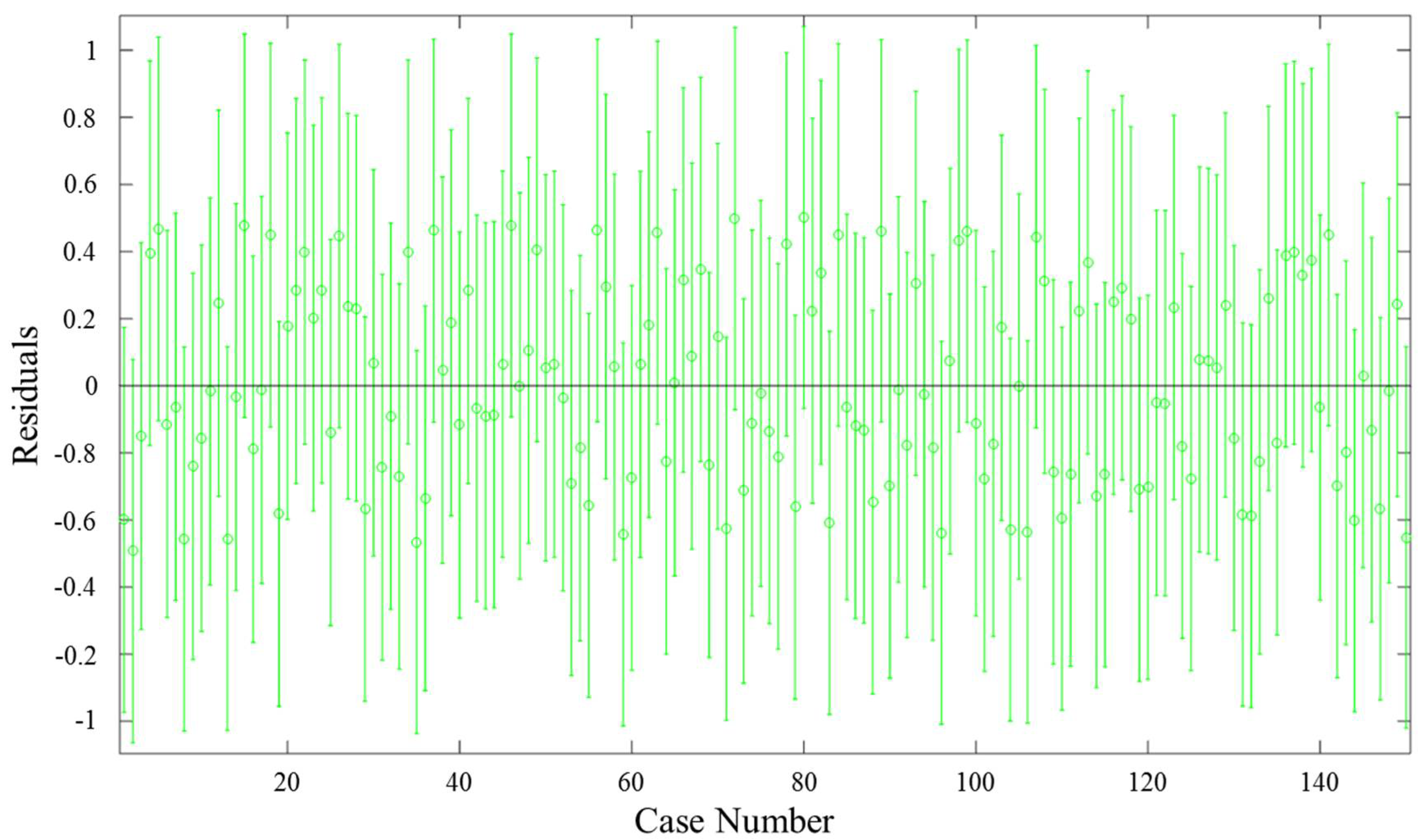
The chiller model was verified by the rest 150 sets of measured data. Figure 1 shows the fitting residual map of the chiller model. Green indicates that the data error is within the allowable range, and red indicates that the data error is out of range.
From Figure 1, it can be seen that the relative errors between the measured values and the predicted values are within the range of 5% in 150 sets of data. The error variance and the correlation coefficient of the fitted model were 0, 1 respectively, which indicated that the fitted model was able to predict the measured data accurately. Therefore, the chiller model was qualified to be used in the subsequent study.
Similarly, the models for the other equipment were accuracy because their residuals were all less than 5%. The models of the other equipment are as follows.
3.2. Mathematical Model between Chilled Station’s Output Cooling Capacity and Equipment Power
The “output cooling capacity-equipment power” (hereinafter referred to as “Cooling capacity—Power”) model of the chilled station were established as follows:
where is the output cooling capacity(kW), N1 is the chiller’s actual power(kW), N2 is the chiller water pump’s actual power (kW), N3 is the cooling water pump’s actual power(kW), N4 is the cooling tower’s actual power(kW), and A/B/C/D/E/F/G/H/I are the model parameters.
Using the 400 sets of measured data, the parameters of the “Cooling capacity-Power” model were determined, the results are as follows.
Therefore, the “Cooling capacity-Power” model is as follows.
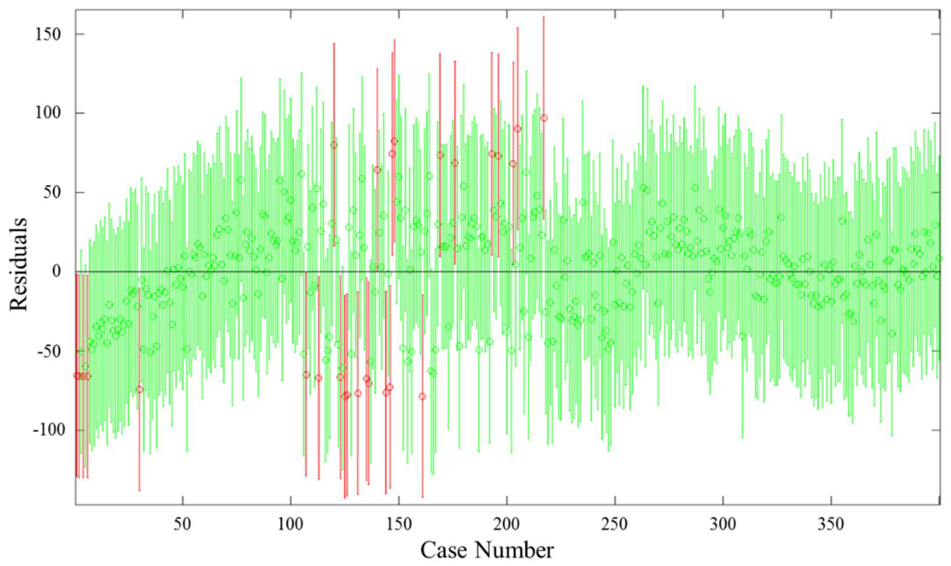
Figure 2 presents the fitting residual map of the “Cooling capacity-Power” model, in which green lines and circles indicate that the data errors are within the range and red lines and circles indicate that the data errors are out of the range. It can be seen that 94.5% of the data were fitted precisely.
3.3. Optimized Control Strategy of Chilled Station
The (PID) control model are widely used in the air conditioning engineering automatic control system because of its simple and stable structure. The PID control of the primary pump variable flow system enables the linear system chilled station to have a certain self-adaptive capacity in dealing with the changes in the building load. However, the central air conditioning system is nonlinear, serious hysteresis phenomenon will happen if the PID control mode is used in the central air conditioning system, further the system has low control efficiency when the building load changes dramatically. In order to resolve this issue, an optimal control strategy based on the “Cooling capacity-Power” model was established in this study.
The device contribution rate refers to the ratio of the amount of changes in cooling capacity to the amount of power changes in a device when any variation occurs in cooling capacity. For example, when it comes to a single chiller, the rated cooling capacity is 500 kW and the rated power is 300 kW. When the cooling capacity reduces from 500 kW to 480 kW, the power of the chiller drops down from 300 kW to 290 kW. The contribution of the chiller is
There is no control module if the system consists of one chiller, one water pump and one cooling tower, and the cooling capacity of the chilled station plunges from 957 kW to 937 kW as well. The measured cooling capacity and power of each device are shown in the Table 6.
From Table 6, it can be seen that when the cooling capacity is 937 kW, the ratio of the cooling capacity to the total input power of the chilled station equipment (chilled station COP) is 3.61. The contribution rate of the chiller is the lowest, and the cooling water pump equipment has the highest contribution rate. Therefore, the cooling capacity can be kept as 1200 kW by increasing input power of the chiller and reducing the input power of the cooling water pump.
The energy consumption of the cooling tower is closely related to the outdoor weather conditions. The cooling water contacts the air in the cooling tower; the sensible heat can be taken by the heat exchange, and the potential heat can be taken by the mass exchange, so the energy consumption process of the cooling tower is dynamical and complicated. Therefore, the cooling tower were not considered for simplifying the model in this paper. When the input power changes, the input power of the chilled station is regarded as a fixed value when calculating the energy efficiency of the chilled station.
Matlab software (2014b, MathWorks, Natick City, MA, USA) was used to determine the minimum power value of each device at a given cooling capacity. Cooling capacity is represented by Qcc, chiller power N1, chilled water pump power N2, cooling water pump power N3, chilled water flow G2, cooling water flow G3, difference between chilled water inlet and outlet unit temperature Δt1, and unit temperature of difference between cooling water inlet and outlet Δt2. Objective function is and its equations are shown in Equation (13), where c = 4.186kJ/(kg °C), ρ = 1000 kg/m3.
There are six variables G2, G3, Δt1, Δt2, k2, and k3 in the objective function, the input power variation range of each equipment and the variation range of the temperature difference between the frozen/water inlet and outlet units are determined according to the actual measurement results. When the cooling capacity is 937 kW, the constraints are as follows:
The optimal value and the result obtained by Matlab are shown in Table 7.
The input power and equipment contribution rate of each device after optimization can be calculated through the Equation (13) and Table 7. The results are shown in the Table 8. These results also indicate that it ensures the cooling capacity is 937 kW and the total input power of the device is the minimum when the input power in Table 8 are used for each equipment.
The chilled station COP is 3.63 using the optimal control strategies, which is 0.55% higher than the previous state. But it can be observed that the device contribution rate of the equipment is basically the same. The observation also can be verified by numerical method. The optimal value of device contribution rate are shown in the Table 9 when the cooling capacity dropping from 957 kW to 917 kW, 897 kW and 877 kW.
The results in the Table 9 present that when cooling capacity is unchanged, optimal value of device contribution rate is the same, In the case of a certain amount of, and the contribution rate of the varies devices of chilled station is the same, the energy consumption of the station reaches its minimum and the operating energy efficiency ratio is the highest. Under the condition that the contribution rate of the equipment of the chilled station stays the same, and the cooling capacity appears to be 917 kW, 897 kW, and 877 kW, the COP of the station goes up by 0.66%, 0.79% and 0.78% respectively.
With seasonal energy efficiency ratio (SEER) as the objective function, a new chilled station operating strategy can be established combined with the “Cooling capacity-Power” model.
Taking into account the known “Cooling capacity-Power” model, the device contribution rate of the equipment is as Table 10.
When the device contribution rate is the same, there is , therefore
The chilled station control strategy is as follows
- The cooling load changes with the variation of outdoor weather conditions, i.e., the cooling capacity is known.
- Combining the Equations (12) and (14), the input power of chilled station equipment can be obtained.
- According to the “power-frequency” model of the equipment obtained in Section 3.1, the equipment frequency can be calculated.
- The device frequency should be adjusted according to the calculation result.
After obtaining the equipment mathematical models, a device customization module can be set up in the TRNSYS simulation platform. The control strategy and the device contribution rate can be considered simultaneously when simulating the energy consumption of the chilled station in the TRNSYS simulation platform.
4. TRNSYS Simulation Platform of Chilled Station Based on Device Contribution Rate
The chilled station operation or optimization? model was established in the TRNSYS simulation platform, which consists of a building cooling load module, a device customization module, a Matlab control module, a weather file input module, and a result output module.
4.1. Building Cooling Load Module
Walls, windows and internal heat source are modeled in the Type56 module, which builta building cooling load model.
4.1.1. Architectural Basic Information
The building tested is an office building, in which the offices and meeting rooms are all air-conditioned, while the corridors and elevator rooms are not. The building is 84 m high, with the roof heat transfer coefficient of 1.96 W/(m2·K), and the external wall heat transfer coefficient of 1.18 W/(m2·K). The window-wall ratio is 0.29 in the north, 0.37 in the south, 0.06 in the west, and 0.06 in the east; in addition, the heat transfer coefficient of the external window is 4.8 W/(m2·K). The external wall area of air-conditioned and non-air-conditioned venues are shown in Table 11.
4.1.2. Architectural Related Parameters
The opening duration of the chilled station of the test building is from 1 July to 30 September each year, a total of 92 days. It runs 5 days a week and the daily operation time is 8:30–17:30.
The USE Weekly Planning Mode is applied to come up with the schedule in the TRNSYS model, in which Monday to Friday are working days, and Saturday and Sunday are resting days. Working hours on weekdays are set at 8:30–17:30. The meaning of USE is: output is 1 during working hours, otherwise 0. The initial temperature of the air-conditioned zone was set at 20 °C, and the initial relative humidity was set at 50%.
The number of people, labor intensity, equipment, lighting, and lighting density are set in light with the actual conditions.
4.1.3. An Analysis on the Temperature and Load of the Building Cooling Load Module
The simulation time of the chilled station was 4344 h to 6552 h in TRNSYS based on the cooling season. Assembly-Control cards were selected in the TRNSYS operation interface to change the simulation time; and the temperature of output interface display was adjusted from 0 to 40 °C. The temporary change graphs of temperature and cooling load can be output after the online plotter is connected.
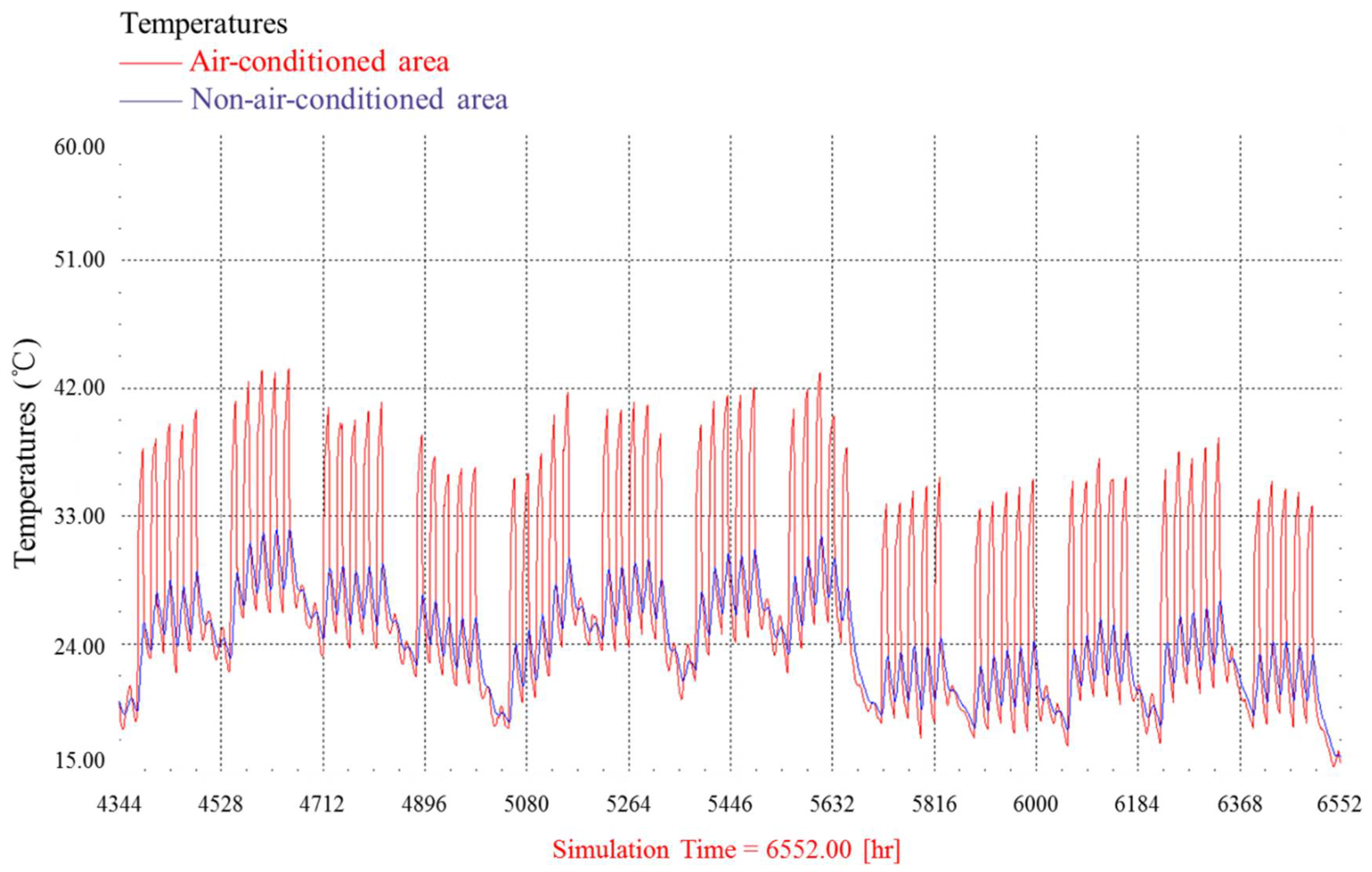
Figure 3 shows the temporary temperature change of the room in the cooling season when the air is not cooled off. Red curves indicate air-conditioned area and blue curves the non-air-conditioned area.
- The total average temperature during 4344~5632 h, is higher than the partial average temperature during 5632~6552 h, which shows the outdoor temperature in July and August is higher than that in September.
- Air-conditioned zone has higher temperature than non-air-conditioned zone. And the former appears people and equipment loads, wherein the internal heat source outnumbers that in the non-air-conditioned zone.
- The temperature curves have obvious patterns, which presents the two wavelet peaks and five large wave peaks are repeated in one cycle. Two wavelet peaks are the hottest in the afternoon on Saturday/Sunday and the five big crests reach their extreme in the afternoon from Monday to Friday. The peaks from Monday to Friday are significantly higher than that on Saturday/Sunday, which can be explained by the situation that there is no personnel and equipment load on Saturday/Sunday, and that the temperature is low, which is consistent with the USE plan stipulated in the Schedule.
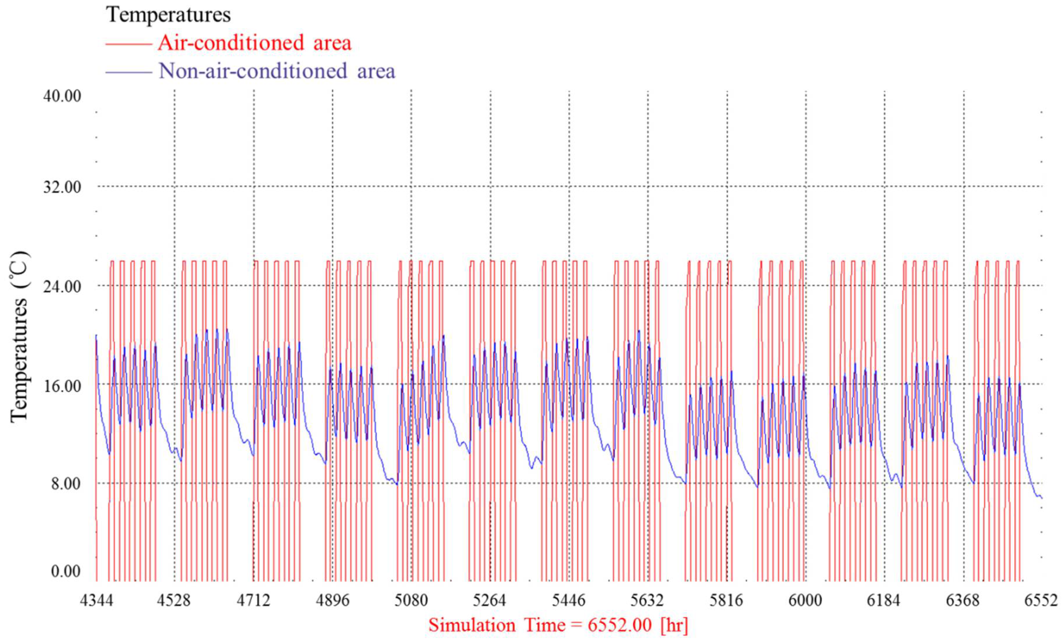
Figure 4 shows the temporary change of the room temperature in the cooling season during cooling period. The room temperature in air-conditioned area stays at 26 °C during the daytime and decreases at night, which can satisfy the USE plan in Cooling.
From the above analysis, it can be concluded that the building model in Type56 was well established due to the consistency between the simulation results and the actual situation.
4.2. Chilled Station Equipment Customization Module
When setting up a chiller module in the TRNSYS simulation platform, the established mathematical model for the chilled station equipment was used to replace the model contained in the software. The model was programmed to create a custom module embedded in the TRNSYS simulation platform.
4.2.1. Chiller Module
The operation parameters of chiller include chilled water inlet unit temperature Tchi, chilled water outlet unit temperature Tcho, chilled water flow Gch, cooling water inlet unit temperature Tci, cooling water outlet unit temperature Tco, cooling water mass flow Gc, chiller operation energy efficiency COP, operating power Pchiller, cooling capacity Qcc, rated cooling capacity Qch, and cooling load Qload. Apart from that, a model identification parameter k1 and a chiller control signal Sc are also a consisting part of the Chiller.
Custom module in TRNSYS was integrated with three tabs that were required to be set: model parameters, input parameters and output parameters, which are as shown in Table 12.
- Modeling steps
A chiller module Type250 that can be applied for TRNSYS simulation was established after the various parameters as custom chiller module required have been determined. The steps are as follows.
- All variables are set based on the analysis results of the chiller operating parameters, and the module was saved as “Type250.tmf”.
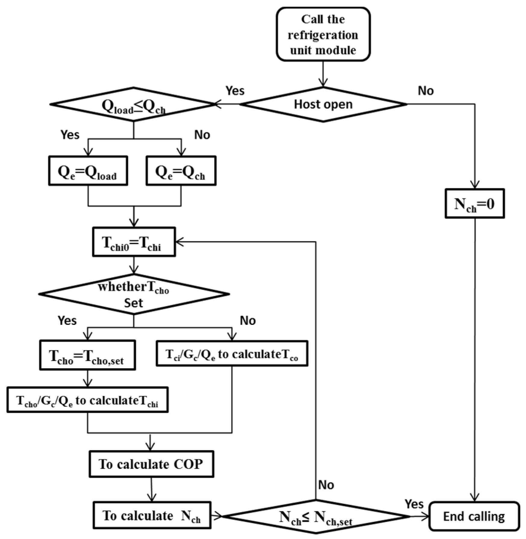
- The C++ program framework was introduced and the calculation program was established for the chiller module, the flow chart of thecustom chiller module program is shown in Figure 5.
- After changing the source program, “Type250.dll” was generated under the directory of “/Trnsys/UserLib”, and so TRNSYS loads the file. Update “Direct Access/Refresh tree”, so that it shall appear in the component module tree on the right side of the interface. Afterwards, the chiller module was established and can be directly called during simulation.
- Verification of module accuracy
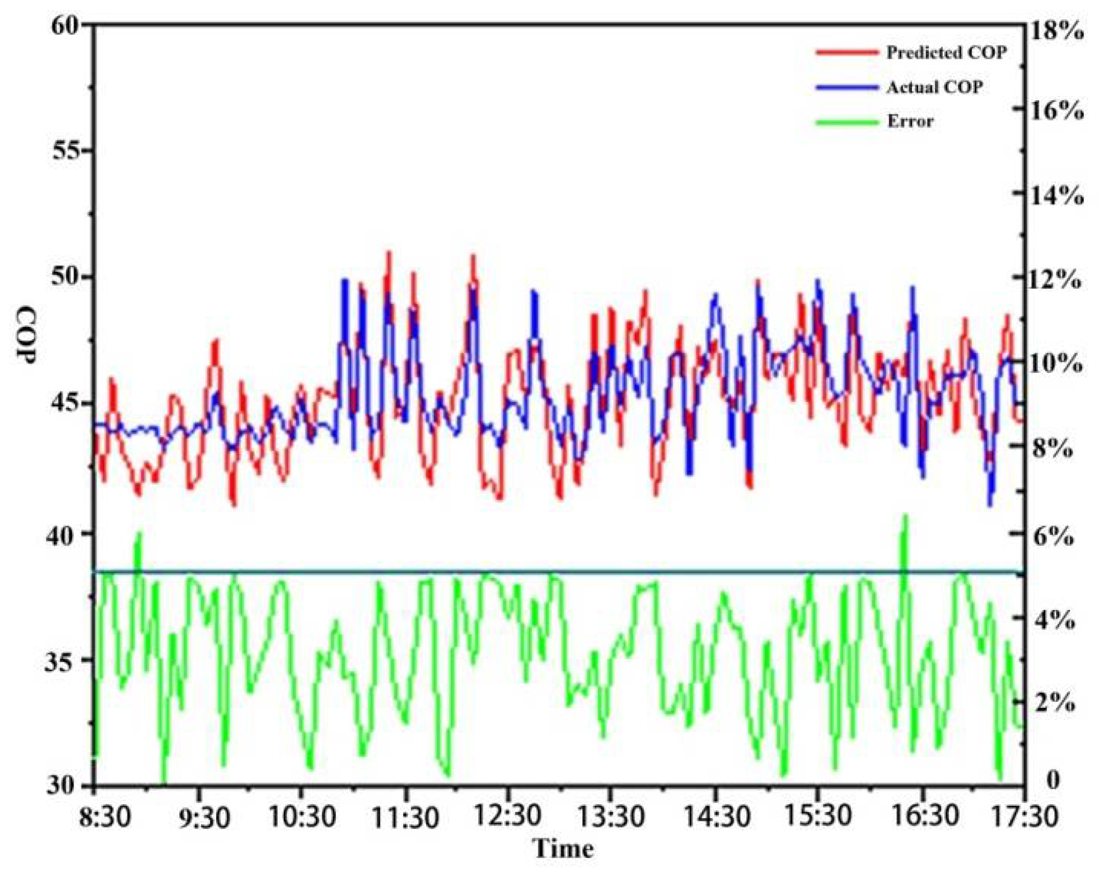
Taking a single chiller as an example, the cooling load, the flow rate of chilled/cooling water, and the return temperature of chilled/cooling water served as input parameters. The chiller module shown in Figure 6 was used to predict the COP and other parameters of the chiller. In Figure 6, red curve represents the predicted value, blue curve represents the actual value, and green curve represents the error. Select 109 sets of operation data on 23 July 2017, which was applied to verify the accuracy of the chiller module.
There were only 2 points where the module prediction COP and the actual COP error were greater than 5%, that is, in 98.16% of the cases, the COP prediction accuracy of the chiller module is above 95%.
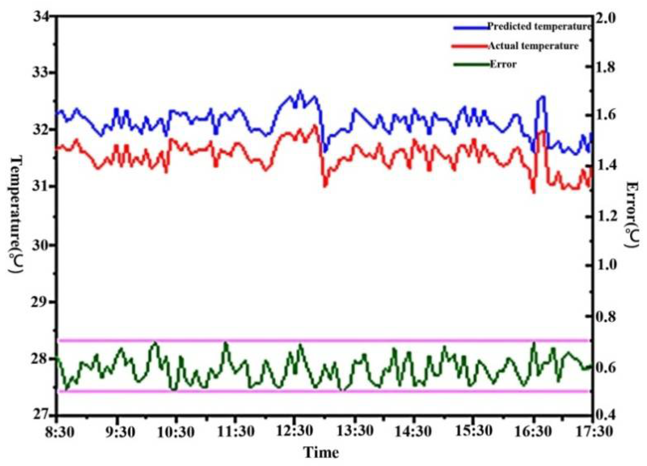
Figure 7 was the cooling water outlet temperature predicted by chiller module. The module predicted that the cooling water outlet temperature of the chiller was lower than the actual temperature, which was due to the cooling water did not absorb heat from the outside during modeling, and the actual condensing heat of the chiller was higher than the sum of the chiller power and cooling capacity. On the ground of that, the actual outlet water temperature was generally high. The difference of cooling water outlet temperature between the predicted and actual values of the module was within the range of 0.5 to 0.7 °C.
It can be concluded that the accuracy of the chiller module is sufficient high; therefore, it can be used for the following simulation from the above analysis results.
4.2.2. Module of Chilled Water Pump
The method of building the water pump module wasquit similar to that of building the chiller. The required parameters are shown in Table 13.
The relevant operation parameters of water pump include inlet water temperature Ti, outlet water temperature To, flow rate G, frequency k, head H, efficiency η, power N, model identification parameters k, G and control signal S.
4.2.3. Cooling Tower Module
The relevant operation parameters of cooling tower cover tower inlet temperature Tco, outlet tower temperature Tci, cooling water flow rate Gc, fan frequency k, model identification parameter k, and control signal S, which can be seen in Table 14.
4.2.4. Matlab Control Module
In line with the chilled station control strategy based on the device contribution rate, the Matlab control module was programmed, and the communication between TRNSYS and Matlab was carried out through the COM interface. Matlab compiles the m file into a COM component, and TRNSYS can directly call the above mentioned m file. When it comes to the TRNSYS simulation, TRNSYS will initially read the start time and end time of the simulation, and the simulation of the step size of the input file was carried through; when calling the m file, TRNSYS simulation would pause and gave time for Matlab to process the result. Matlab simulation ceased at the end of Matlab processing, and TRNSYS read the simulation results and continued to follow out the simulation. The entire process was done alternately until the end of the simulation.
4.3. Chilled Station TRNSYS Simulation Platform
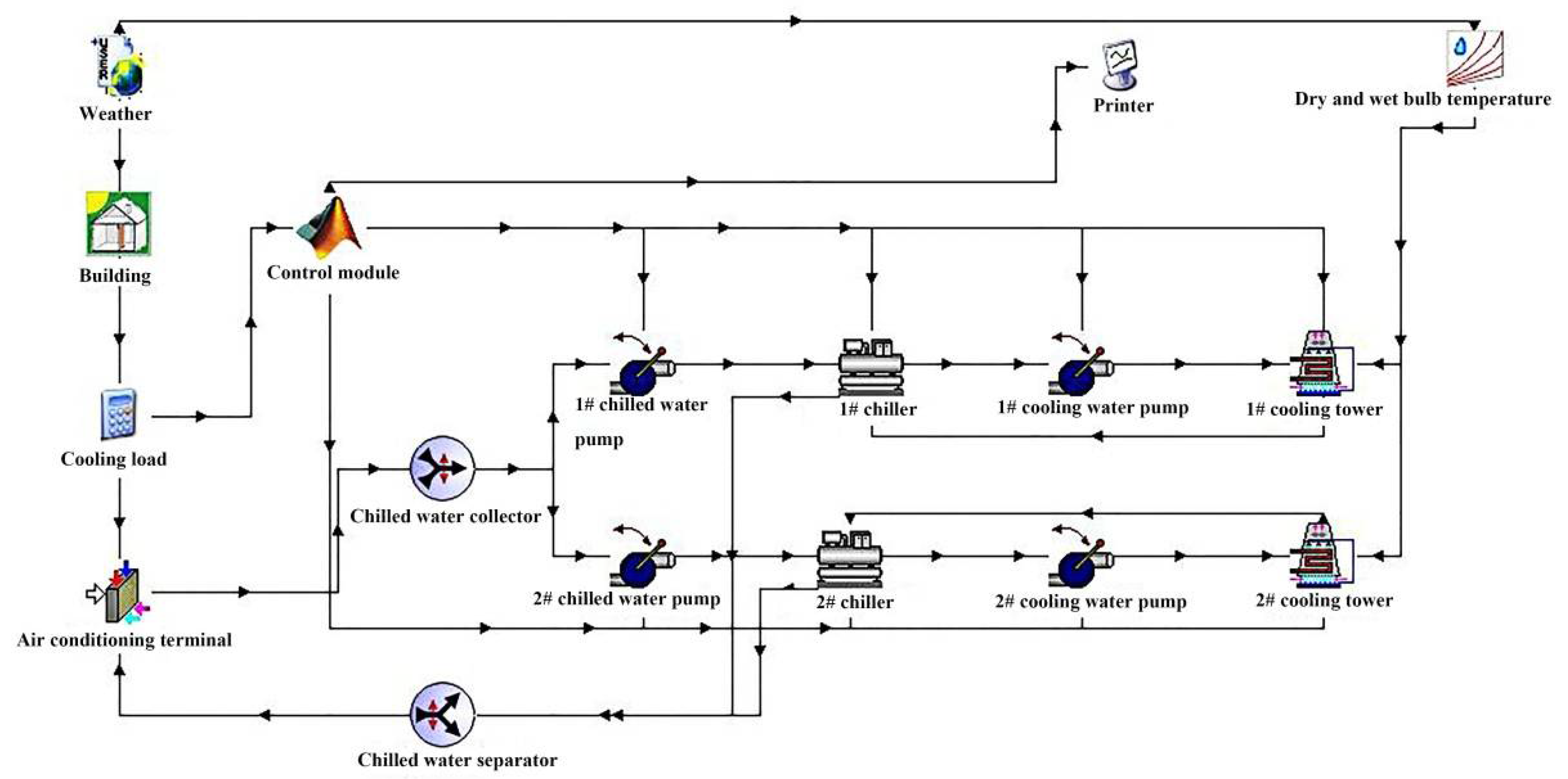
Create an empty project, introduce the selected components to the project, set the parameters of each component in accordance with the previous requirements, connect the components, and establish a simulation platform on the basis of combining operation of TRNSYS and Matlab as Figure 8.
The TRNSYS simulation platform of chilled station had been set up as Figure 8, which can be used to simulate the energy consumption of the chilled station and to calculate the SEER supported by the optimal control strategy.
5. Analysis on the Optimization Effect of Chilled Station Based on SEER
The chilled station’s TRNSYS simulation platform was designed to simulate the energy consumption of the chilled station from 1 July to 30 September (corresponding to the TRNSYS simulation platform 4344~6552 h), and the SEER based on the device contribution rate can be calculated therefrom.
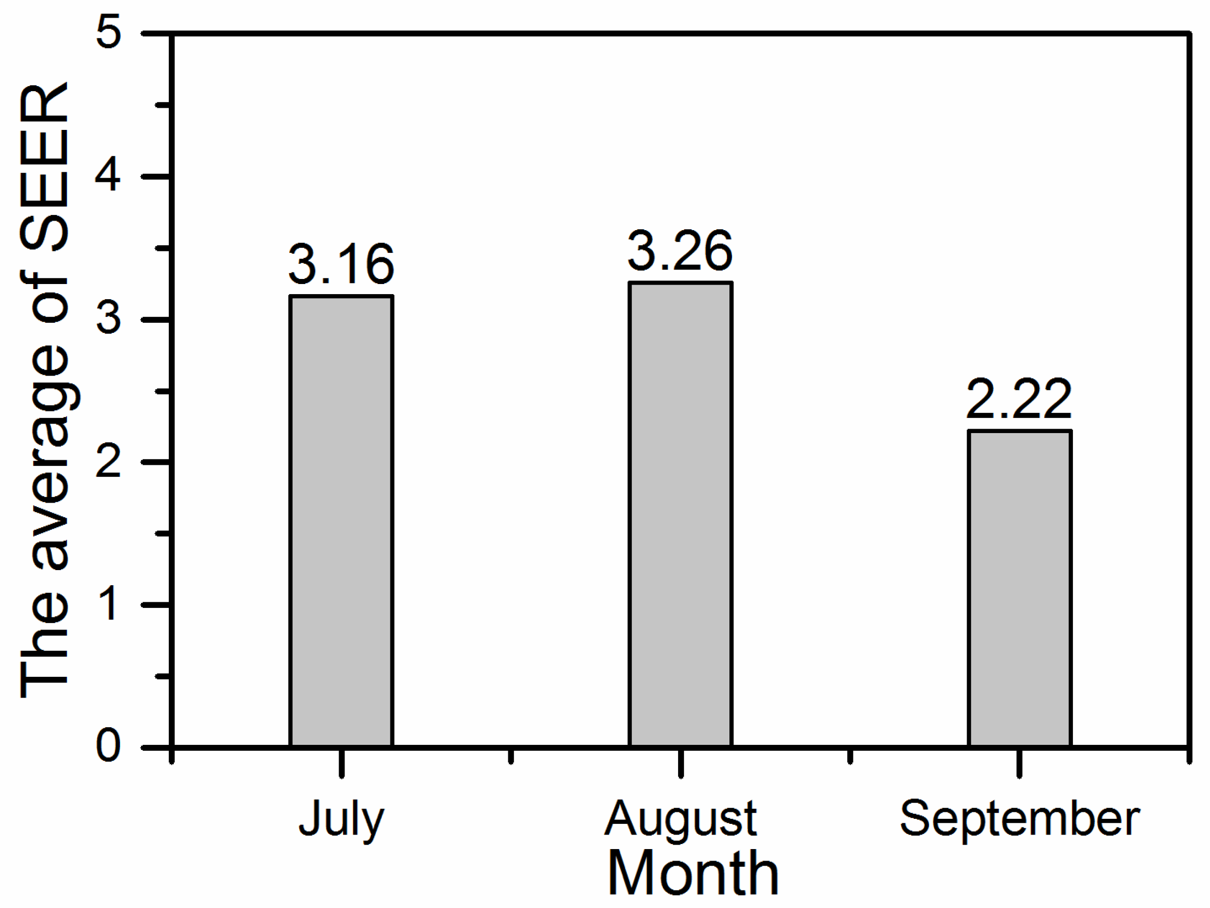
According to the simulation results of the chilled station, the monthly control strategy-based SEER distribution control strategy-based of device contribution rate of the test building was shown in Figure 9.
The test building was simulated using the control strategy based on device contribution rate, the results obtained therefrom suggest that the average SEER during the cooling season is 2.88. The highest average SEER is 3.26 in August, and the lowest is 2.22 in September. Noticeably, the value of SEER based on the device contribution rate is 2.15 times as high as the current SEER, indicating that the control strategy is fairly effective. It is worth to further research and development in this field.
6. Conclusions
An innovative device contribution rate-based chilled station control strategy is proposed in this study, whose TRNSYS model was established to simulate energy consumption. The SEER served as an evaluation index to verify the effectiveness of the control strategy.
- A mathematical model of “chilled capacity—equipment power” of the chilled station was put forward and established with a correlation coefficient of 0.9917, which is
- Matlab was used to determine the power value of each device that can minimize the total power input of chilled station under a given cooling capacity. The optimal value of device contribution rate was the same, and the chilled station COP increased by 1.80%, 0.96%, and 1.65% in the circumstances where the cooling capacity was 1180 kW, 1160 kW, and 1140 kW. Under a certain amount of cooling capacity, the energy consumption of the chilled station reached to the minimum when the device contribution rate stayed the same and the SEER was at its utmost value. To this end, the whole frequency conversion control strategy of the chilled station based on the device contribution rate came into being, and the Matlab control module is loaded into the TRNSYS simulation platform to simulate the performance.
- The actual SEER of test building appears to be 1.34 during the cooling season. The full frequency conversion control strategy of the chilled station built upon the device contribution rate is applied to TRNSYS platform to simulate energy consumption. The simulation result shows that the average SEER is 2.88, which is 2.15 times of the current value.
- Next, operation strategies can be applied in actual projects or experimental stations to conduct experimental analysis to verify the effects.
Author Contributions
M.L. checked the manuscript. C.S. carried out the mathematical models of equipment and the “cooling capacity-power”, established the chilled station TRNSYS platform and finished the original manuscript. B.Z. contacted the site survey. J.W. and Q.D. revised the manuscript. L.L. participated in field tests.
Funding
The National Natural Science Foundation of China (No. 51638003); The Fundamental Research Funding for Central Universities (No. DUT17RW118).
Acknowledgments
The authors gratefully acknowledge the National Natural Science Foundation of China (No. 51638003) and the Fundamental Research Funding for Central Universities (No. DUT17RW118) for the cost of research.
Conflicts of Interest
The authors declare no conflict of interest.
References
- Liu, G.D.; Ma, W.W.; Liu, Q.Y. Energy consumption analysis of air conditioning cooling water pumps by variable frequency speed regulation. In Proceedings of the National HVAC Refrigeration 2010 Annual Conference, Hangzhou, China, 8 November 2010. [Google Scholar]
- Shuang, L. Full-frequency conversion and energy-saving analysis of cold station system. Refrig. Air Cond. 2015, 35, 48–51. [Google Scholar]
- Bahnfleth, W.P.; Peyer, E.B. Energy use and economic comparison of chilled-water pumping system alternatives. ASHRAE Trans. 2006, 112, 198–208. [Google Scholar]
- Fangyuan, L. Cooling tower fan frequency control and energy saving. Fan Technol. 2007, 2, 57–59. [Google Scholar]
- Hartman, T. ‘LOOP’ chiller plant dramatically lowers chilled water costs. In Proceedings of the Renewable and Advanced Energy Systems for the 21th Century, Maui, HI, USA, 12 April 1999. [Google Scholar]
- Ou, H.F. Analysis of Air-Conditioning System Design and Energy-Saving Operation of a Commercial Plaza in Foshan. Master’s Thesis, South China University of Technology, Guangzhou, China, 2014. [Google Scholar]
- Yu, J. Research and Implementation of Energy-Saving Control Methods for Central Air-Conditioning in Public Buildings. Master’s Thesis, Beijing University of Architecture, Beijing, China, 2013. [Google Scholar]
- Mo, Y.P. Research on Optimal Configuration and Operation of Air Conditioning System Chillers in a Hospital in Guangzhou. Master’s Thesis, Guangzhou University, Guangzhou, China, 2013. [Google Scholar]
- Tian, Z.; Qian, C.; Gu, B. Electric vehicle air conditioning system performance prediction based on artificial neural network. Appl. Therm. Eng. 2015, 89, 101–114. [Google Scholar] [CrossRef]
- Lim, D.K.; Ahn, B.H.; Jeong, J.H. Method to control an air conditioner by directly measuring the relative humidity of indoor air to improve the comfort and energy efficiency. Appl. Energy 2018, 215, 290–299. [Google Scholar] [CrossRef]
- Zhou, Y. Optimization and Application of Energy Efficiency of Central Air Conditioning Cold Source System in a Shopping Mall. Master’s Thesis, South China University of Technology, Guangzhou, China, 2014. [Google Scholar]
- Wu, S.H. Design and Implementation of Group Control System for Freezer Room. Master’s Thesis, East China University of Science and Technology, Shanghai, China, 2014. [Google Scholar]
- Chen, D.D. Study on Real-Time Optimization Control Strategy of Central Air Conditioning Variable Water System. Master’s Thesis, Shanghai Jiao Tong University, Shanghai, China, 2007. [Google Scholar]
- Ahn, B.C.; Mitchell, J.W. Optimal control development for chilled water plants using a quadratic representation. Energy Build. 2001, 33, 371–378. [Google Scholar] [CrossRef]
- Zhang, L. Research on Energy Saving Reform of a Central Air Conditioning System. Master’s Thesis, Harbin Institute of Technology, Harbin, China, 2013. [Google Scholar]
- Gao, J.; Huang, G.; Xu, X. An optimization strategy for the control of small capacity heat pump integrated air-conditioning system. Energy Convers. Manag. 2016, 119, 1–13. [Google Scholar] [CrossRef]
- Bursill, J.; Cruickshank, C.A. Heat pump water heater control strategy optimization for cold climates. J. Sol. Energy Eng. 2016, 138, 011011. [Google Scholar] [CrossRef]
- Jia, P. Brief analysis of GB19577-2015, Cold energy Efficiency Limit Value and Energy Efficiency Grade of Chillers“. Air Cond. HVAC Technol. 2016, 4, 32–33. [Google Scholar]
- Yang, L.N. Research on Energy Efficiency Ratio of Air Conditioning Projects in Public Buildings. Master’s Thesis, Chongqing University, Chongqing, China, 2007. [Google Scholar]
- Zhang, B.G.; Wang, T.X.; Liu, M. Establishment of chilled water system model based on monitoring data. Low Temp. Build. Technol. 2017, 39, 148–151. [Google Scholar]
Figure 1.
Map of chiller model fitting residual.

Figure 2.
Fitting residual map of “Cooling capacity-Power” model.

Figure 3.
Temperature temporary change without cooling.

Figure 4.
Temporary temperature change with cooling.

Figure 5.
Flowchart of a custom chiller module program.

Figure 6.
Chiller module prediction COP.

Figure 7.
The cooling water outlet temperature of chiller predicted by the module.

Figure 8.
TRNSYS simulation platform of chilled station.

Figure 9.
Monthly SEER based on the control strategy of the device contribution rate.


Table 1.
The nameplate parameters of the equipment of the air condition system.
| Device Name | Nameplate Parameter |
|---|---|
| Chiller | Qch = 1383.2 kW; N = 265.7 kW |
| Cooling water pump | G = 319 m3/h; H = 27 m; r = 1450 r/min; N = 37 kW |
| Cooling tower | G = 320 m3/h; cooling water 37/32 °C; N = 5.5 kW × 2 |
| Chilled water pump | G = 262 m3/h; H = 33 m; r = 1450 r/min; N = 37 kW |
| Fan coil | Total 280.32 kW |
| Variable Refrigerant Volume | Total 435.25 kW |
Table 2.
Energy efficiency rating of water-cooled chiller energy efficiency.
| Nominal Cooling Capacity (CC) kW | Energy Efficiency Rate | |||||
|---|---|---|---|---|---|---|
| 1 | 2 | 3 | ||||
| (COP) W/W | (IPLV) W/W | (COP) W/W | (IPLV) W/W | (COP) W/W | (IPLV) W/W | |
| CC ≤ 528 | 5.60 | 7.20 | 5.30 | 6.30 | 4.20 | 5.00 |
| 528 < CC ≤ 1163 | 6.00 | 7.50 | 5.60 | 7.00 | 4.70 | 5.50 |
| CC > 1163 | 6.30 | 8.10 | 5.80 | 7.60 | 5.20 | 5.90 |
Table 3.
The DEER limits of office buildings in Chongqing.
| Cold Source | Air-Cooled Heat Pump Chiller | Screw Chiller | Screw Chiller | Variable Frequency VRV Air Conditioning System | LiBr Absorption Chiller |
|---|---|---|---|---|---|
| DEER limits | 2.40 | 2.89 | 3.25 | 2.20 | 2.60 |
Table 4.
Mathematical model parameters.
| Model | Parameters |
|---|---|
| Chiller | N1, k1 |
| Chilled water pump | N2, k2, G2 |
| Cooling water pump | N3, k3, G3 |
| Cooling tower | N4, k4, kct |
Table 5.
Symbols and their meanings.
| Symbol | Meaning |
|---|---|
| H2 | chilled water pump head (m) |
| G2 | chilled water pump flow (m3/h) |
| k2 | motor operating frequency of chilled water pump (Hz) |
| η2 | chilled water pump efficiency (%) |
| N2 | chiller water pump’s actual power (kW) |
| H3 | cooling water pump head (m) |
| G3 | cooling water pump flow (m3/h) |
| k3 | motor operating frequency of cooling water pump (Hz) |
| η3 | cooling water pump efficiency (%) |
| N3 | cooling water pump’s actual power (kW) |
| N4 | cooling tower actual power (kW) |
| k4 | motor operating frequency of cooling tower (Hz) |
| kct | rated motor frequency of cooling tower, i.e., 50 (Hz) |
Table 6.
Changing table of the cooling capacity and equipment power of the chilled station.
| Cooling Capacity (kW) | Actual Input Power of Chilled Station Equipment (kW) | |||
|---|---|---|---|---|
| Chiller | Chilled Water Pump | Cooling Water Pump | Cooling Tower | |
| 957 | 214.01 | 19.30 | 24.60 | 6.60 |
| 937 | 209.52 | 18.97 | 24.50 | 5.96 |
| Device contribution rate | 4.45 | 60.53 | 190.56 | 31.25 |
Table 7.
Matlab optimization results.
| Variable | G2 | G3 | Δt1 | Δt2 | k2 | k3 |
|---|---|---|---|---|---|---|
| Optimization value | 201.139 | 247.027 | 4.002 | 3.997 | 42.601 | 25.004 |
Table 8.
Device input power after Matlab optimization.
| Device | Chiller | Chilled Water Pump | Cooling Water Pump |
|---|---|---|---|
| Input power (kW) | 212.14 | 17.43 | 22.73 |
| Device contribution rate | 10.70 | 10.70 | 10.69 |
Table 9.
Device contribution rate under different cooling capacities.
| Cooling Capacity (kW) | Actual Input Power of Chilled Station Equipment (kW) | Chilled Station COP | ||
|---|---|---|---|---|
| Chiller | Chilled Water Pump | Cooling Water Pump | ||
| 917 before fixing | 207.24 | 18.87 | 24.48 | 3.57 |
| Device contribution rate | 5.91 | 93.02 | 330.49 | |
| 917 after fixing | 211.01 | 16.30 | 21.60 | 3.59 |
| Device contribution rate | 13.33 | 13.33 | 13.33 | |
| 897 before fixing | 206.96 | 18.66 | 23.97 | 3.50 |
| Device contribution rate | 8.51 | 93.75 | 95.08 | |
| 897 after fixing | 210.57 | 15.86 | 21.16 | 3.53 |
| Device contribution rate | 17.44 | 17.44 | 17.44 | |
| 877 before fixing | 205.59 | 18.32 | 23.92 | 3.45 |
| Device contribution rate | 9.50 | 81.63 | 117.47 | |
| 877 after fixing | 209.99 | 15.28 | 20.58 | 3.47 |
| Device contribution rate | 19.90 | 19.90 | 19.90 | |
Table 10.
Device contribution rate of chilled station equipment.
| Device | Device Contribution Rate |
|---|---|
| Chiller | |
| Chilled water pump | |
| Cooling water pump | |
| Cooling tower |
Table 11.
External wall area in all directions.
| Area | External Wall Area (m2) | |||
|---|---|---|---|---|
| North | South | West | East | |
| Air-conditioned area | 2066.4 | 2688 | 1142.4 | 1411.2 |
| Non-air-conditioned area | 621.6 | 0 | 705.6 | 436.8 |
Table 12.
Custom chiller module parameters.
| Model parameters | N, Qch, k1 |
| Input parameters | Tchi, Tci, Gch, Gc, Qload, S |
| Output parameters | Tcho, Tco, Gch, Gc, COP, Qcc, Pchiller |
Table 13.
Parameters of custom chilled water pump module.
| Parameters | Chilled Water Pump | Cooling Water Pump |
|---|---|---|
| Model parameters | Rated power Nch, rated flow Gch, rated head Hch, model identification parameters | Rated power Nc, rated flow Gc, rated head Hc, model identification parameters |
| Input parameters | G2, k2, S | G3, k3, S |
| Output parameters | N2, η2, H2 | N3, η3, H3 |
Table 14.
Parameters of custom cooling tower module.
| Model parameters | Rated power Nct, rated flow Gct, rated frequency kct, model identification parameters |
| Input parameters | G3, k4, S |
| Output parameters | N4 |
© 2018 by the authors. Licensee MDPI, Basel, Switzerland. This article is an open access article distributed under the terms and conditions of the Creative Commons Attribution (CC BY) license (http://creativecommons.org/licenses/by/4.0/).
Share and Cite
MDPI and ACS Style
Liu, M.; Sun, C.; Zhang, B.; Wang, J.; Duan, Q.; Lv, L. Optimized Operation of an Existing Public Building Chilled Station Using TRNSYS. Buildings 2018, 8, 87. https://doi.org/10.3390/buildings8070087
AMA Style
Liu M, Sun C, Zhang B, Wang J, Duan Q, Lv L. Optimized Operation of an Existing Public Building Chilled Station Using TRNSYS. Buildings. 2018; 8(7):87. https://doi.org/10.3390/buildings8070087
Chicago/Turabian StyleLiu, Ming, Chang Sun, Baogang Zhang, Julian Wang, Qiuhua Duan, and Lin Lv. 2018. "Optimized Operation of an Existing Public Building Chilled Station Using TRNSYS" Buildings 8, no. 7: 87. https://doi.org/10.3390/buildings8070087
Note that from the first issue of 2016, this journal uses article numbers instead of page numbers. See further details here.