Daylight Discomfort Glare Evaluation with Evalglare: Influence of Parameters and Methods on the Accuracy of Discomfort Glare Prediction


1
Université catholique de Louvain, 1348 Louvain-la-Neuve, Belgium
2
École Polytechnique Fédérale de Lausanne, 1015 Lausanne, Switzerland
*
Author to whom correspondence should be addressed.
Buildings 2018, 8(8), 94; https://doi.org/10.3390/buildings8080094
Submission received: 26 June 2018
/
Revised: 17 July 2018
/
Accepted: 17 July 2018
/
Published: 24 July 2018
(This article belongs to the Special Issue Advances in Discomfort Glare Research)
Abstract
:Nowadays, discomfort glare indices are frequently calculated by using evalglare. Due to the lack of knowledge on the implications of the methods and parameters of evalglare, the default settings are often used. But wrong parameter settings can lead to inappropriate glare source detection and therefore to invalid glare indices calculations and erroneous glare classifications. For that reason, this study aims to assess the influence of several glare source detection methods and parameters on the accuracy of discomfort glare prediction for daylight. This analysis uses two datasets, representative of the two types of discomfort glare: saturation and contrast glare. By computing three different statistical indicators to describe the accuracy of discomfort glare prediction, 63 different settings are compared. The results suggest that the choice of an evalglare method should be done when considering the type of glare that is most likely to occur in the visual scene: the task area method should be preferred for contrast glare scenes, and the threshold method for saturation glare scenes. The parameters that should be favored or avoided are also discussed, although a deeper understanding of the discomfort glare mechanism and a clear definition of a glare source would be necessary to reliably interpret these results.
1. Introduction
According to the International Commission on Illumination (CIE), glare is defined as the “condition of vision in which there is discomfort [discomfort glare] or a reduction in the ability to see significant objects [disability glare], or both, due to an unsuitable distribution or range of luminances or to extreme contrasts in space or time” [1]. When studying discomfort glare nowadays, the most common method is to compare subjective glare ratings that are made on discomfort glare scales, and the values of discomfort glare indices calculated from measured physical quantities. There are four main physical quantities, on which discomfort glare indices are based [1]: the luminance of the glare source(s) in the field of view, the solid angle of the glare source(s), the luminance of the background, and the position index of the glare source(s). To measure these quantities efficiently in situ, High Dynamic Range (HDR) imaging technique is used to create a 180° luminance map containing the subject’s field of view. Discomfort glare indices are then calculated afterward on the basis of these luminance maps. Alternatively, such 180° luminance maps can also be generated through simulation tools. The calculation of discomfort glare indices based on a luminance map is therefore an essential step and an inherent part of discomfort glare studies.
The difficulty of this step, however, lies in the identification of the glare source(s) in the field of view. If a glare source has been identified in the 180° luminance map, its solid angle, position index, and luminance can be easily determined. The background luminance can also be quickly evaluated as the average luminance of the luminance map, excluding the glare source. But, as reported in [2], the definition of the glare source is still ambiguous, and there is no universal method of identifying one. The most common methods that are currently used are the ones implemented in evalglare. Evalglare is a Radiance-based tool developed by J. Wienold as part of a larger glare study with J. Christoffersen [3], during which they created the Daylight Glare Probability (DGP) index. This tool requires a 180° luminance map containing the field of view as input, then runs an algorithm to detect glare sources, and finally calculates different discomfort glare indices from the detected glare sources [4,5,6]. The output of evalglare is therefore a list of discomfort glare indices values that are calculated on the basis of the glare sources detected by the algorithm in the luminance map. Evalglare is a powerful tool that makes discomfort glare indices calculations easier and quicker, which is the reason why it is so widely used.
Evalglare algorithm enables the use of three different methods for glare source detection: the factor method, the threshold method, and the task area method, which will be explained later. The task area method is the one that provided the best results for Wienold’s study [7] in terms of correlation with subjective glare ratings. However, the factor method is more widely used, as a consequence of being the default method implemented in evalglare. What is more, the factor method is also the default method when performing a point-in-time glare analysis in the daylight-simulation software DIVA-for-Rhino [8], and there exists no option in the user-friendly interface to modify it.
Moreover, several options and parameters can be changed in evalglare, which modify the glare source detection algorithm. But, these options and parameters are seldom used as compared to the default or recommended ones, probably because of the lack of knowledge about their influence on glare sources detection. Surprisingly, evalglare tool has never been the object of a validation study—other than Wienold and Christoffersen’s study—although it has been now used for over 10 years. There exist no recommendations based on scientific evidence on which methods should be preferred in which cases, and which options should be applied for which conditions.
Therefore, the aim of this study is to investigate the effect of different evalglare methods and parameters on discomfort glare prediction. Although it would be interesting to look at the sensitivity of discomfort glare indices values when varying evalglare methods and parameters, the focus of this study is about determining which method and parameters offer the best discomfort glare prediction in comparison with subjective glare ratings. Two datasets are used in this study, comprising, for each glare evaluation, a subjective glare rating and a 180° luminance map containing the subject’s field of view. Each dataset is representative of a discomfort glare type, i.e., contrast glare or saturation glare. By varying evalglare options—combination of evalglare methods and parameters—when calculating the discomfort glare indices based on the luminance maps, the options that offer the best prediction of subjective glare ratings for the two types of glare may be identified.
2. Datasets
Two datasets containing daylight discomfort glare evaluations are used for this study. The demographic information of these datasets is available in Table 1.
The first dataset was collected during a field study that was conducted in Louvain-la-Neuve (Belgium) from June to August 2017. 82 subjects participated in the study, which consisted of collecting almost simultaneously subjective glare ratings and 180° luminance maps containing the subject’s field of view in their real office. The study took place in several university buildings, for office desks that are located next to an east-, west-, or south-oriented window. Each subject did two glare evaluations—the first one for the situation they were working in, and the second one for the situation with opened shading devices and artificial lighting turned off—resulting in a total of 164 evaluations. Despite the fact that the field study was conducted under clear sky conditions, 23 evaluations had to be disregarded due to unstable lighting conditions. The subjective glare ratings were preceded by a short visual task, and were made on a 4-point scale, on which the subject has to evaluate his/her perception of discomfort due to glare as either “No discomfort”, “A small discomfort”, “A moderate discomfort”, or “A large discomfort”. The detailed experiment protocol has been published in [9].
The second dataset was collected during a laboratory study that was conducted in two office-like cells in Freiburg (Germany) in the spring/summer/autumn months between 2008 and 2011. In total, 150 subjects had to perform five visual tasks, each followed by a discomfort glare rating, for maximum four different visual scenes—the shading device was varied—at two different times of the day—morning and afternoon. However, only data from 41 subjects and from one of the five visual tasks, namely the typing task, collected in the spring and summer months were available and used in this study, resulting in a total of 180 glare evaluations. The laboratory study was conducted under clear sky conditions, and the office-like cells were rotated so that the sun direction was perpendicular to the façade. The discomfort glare rating was done on a different 4-point glare scale, on which the subject was asked to evaluate his/her glare perception as “Imperceptible”, “Noticeable”, “Disturbing”, or “Intolerable”. Simultaneously with the discomfort glare rating, a 180° luminance map was created with the luminance camera positioned next to the subject’s head, at eye level. More details about this laboratory study have been published in [10].
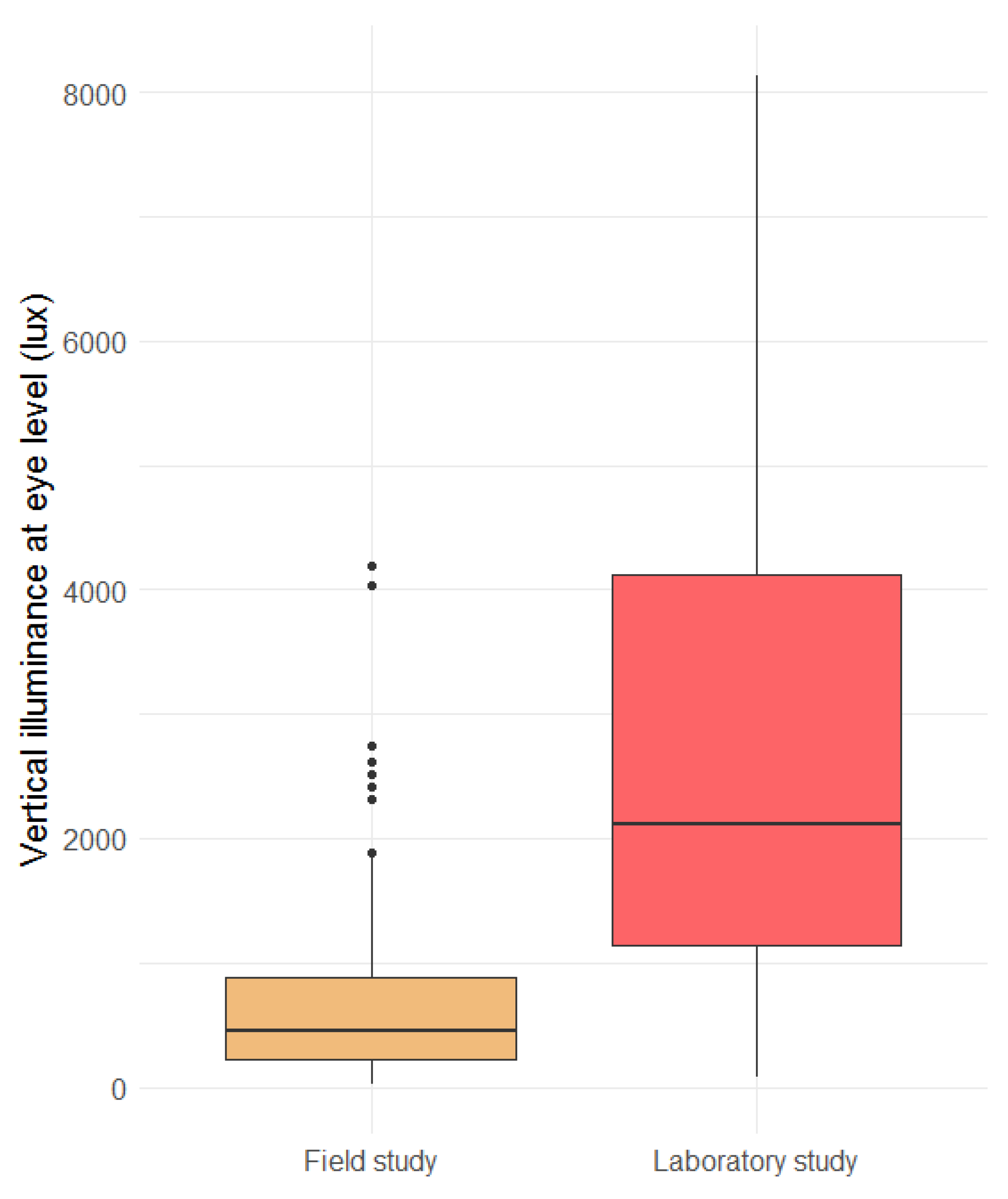
The choice of using two different datasets was made so that a greater variety of visual scenes is studied, especially the two types of discomfort glare, namely the contrast and saturation glare. The lighting conditions between the two studies are very different, as can be seen in Figure 1. Vertical illuminance at the eye level is much higher in the case of the laboratory study, with a median illuminance level above 2000 lux, when compared to a median illuminance level of around 500 lux for the field study. This implies that when discomfort glare was perceived in the field study, discomfort most probably was caused from high contrast between the glare source and the background. On the opposite, when discomfort glare was perceived in the laboratory study, discomfort was most probably due to a too bright visual scene. Therefore, most discomfort glare situations in the field study were caused by contrast glare, whereas discomfort glare situations in the laboratory study were mainly caused by saturation glare. These two datasets can therefore be used as the representatives of the two main types of discomfort glare. Moreover, the two studies have several differences in their experimental design, besides being a field or laboratory study type. One of the main differences is the use of two different glare rating scales for the subjective evaluation of discomfort glare (Table 1). Another main difference is that, in the field study, the HDR image is captured directly after the subjective glare rating, but at the exact same place of the subject’s eyes, while in the laboratory study, the HDR image is captured at the exact same time than the subjective glare rating, but next to the subject’s head. These differences make the two datasets representative of many discomfort glare studies, and they enable the results to be relevant for a large number of future studies. These differences also hinder the comparison of the accuracy of discomfort glare prediction between the datasets, which is not the subject of this study.
3. Methodology
When using evalglare, the choice of a method and parameters influence glare source detection in a luminance map. The detected glare sources, in turn, influence discomfort glare indices calculation. At last, the accuracy of discomfort glare prediction varies according to these discomfort glare indices. To determine which method and which parameters of evalglare are the most appropriate for each type of discomfort glare research, the reported effects of the choice of a method and parameters in evalglare on the accuracy of discomfort glare prediction is investigated. However, the effects of this choice on the in-between steps, namely the glare source detection and the discomfort glare indices calculation, will not be examined here.
63 different evalglare options—each option is a different combination of one of the three evalglare methods and different parameters—for detecting glare sources in a luminance map are tested. The accuracy of discomfort glare prediction of these 63 different options is evaluated through three different statistical approaches for each of the two datasets. The 63 studied evalglare options, as well as the three statistical approaches are explained in Section 3.1 and Section 3.2.
3.1. Studied Evalglare Methods and Parameters
The three different methods implemented in evalglare are, as named in this article, the factor method, the threshold method, and the task area method.
The algorithm of the factor method detects in the 180° luminance map all of the pixels having a luminance value higher than the mean luminance of the luminance map multiplied by a certain factor. These pixels are treated as the glare sources. In this study, 4 different factors were tested: a multiplying factor of 5 (b5), which is the default method in evalglare, 6 (b6), 7 (b7), and 8 (b8).
The algorithm of the threshold method detects in the 180° luminance map all pixels having a luminance value that is higher than a certain threshold, and treat these pixels as the glare sources. In the literature, several thresholds have been used throughout the years [11,12,13,14,15], but the three most common ones are a threshold of 1000 cd/m2 (b1000), of 2000 cd/m2 (b2000), and of 4000 cd/m2 (b4000).
The algorithm of the task area method detects in the 180° luminance map all pixels having a luminance value higher than the mean luminance of a defined task area in the luminance map multiplied by a certain factor. This last method requires prior definition of a task area. The recommended multiplying factor for the task area method in evalglare is 5. Three other factors will also be tested in this study, resulting in multiplying factors of 3 (t3), 4 (t4), 5 (t5), and 6 (t6).
Four other evalglare parameters are investigated in this study. First, the background luminance definition will be tested, since there exist two different definitions of this background luminance. The first definition is the one that is provided by the CIE, which approximates the background luminance as the indirect vertical illuminance of the visual field divided by π (_def). The second one is the mathematical definition, i.e., the mathematical average of the luminance values in the luminance map excluding the glare sources (_Lb). Secondly, the search radius, which is the distance within which two glaring pixels are included in the same glare source, will be varied. The default value of the search radius, 0.2 (_def), as well as one smaller value −0.06 (_r0.06)—and one larger value −0.3 (_r0.3)—will be tested. The task area size, which is only required when using the task area method, will then be varied as well. The task area is defined as the area where the subject’s eyes are focused. The usual task area size has an opening angle of around 60° (_def) to correspond to the ergorama, i.e., the area around the computer screen and keyboard. A smaller task area size −30° (_ta0.52)—including only the computer screen, and a larger size −90° (_ta1.57)—will also be tested. At last, the smooth parameter, which should mainly be used when the visual scene includes blinds, is investigated. This parameter includes non-glaring pixels (pixels of blind slats for instance) nested in a glare source (a glare source seen through the blinds for instance) to the glare source, smoothing the glare source area. The accuracy of discomfort glare prediction will thus be tested with (_sm) and without (_def) the smooth parameter.
Table 2 summarizes all 63 evalglare options that were tested in this study and provides an example of the differences in glare sources detection between these options. The colored parts in the images correspond to the different detected glare sources. The choice of colors is randomly made by evalglare algorithm and has no signification.
3.2. Statistical Approaches
Instead of looking at the direct effects of the 63 different evalglare options on glare source detection or on discomfort glare indices calculation, the reported effects on the accuracy of discomfort glare prediction is studied. The accuracy of discomfort glare prediction can be defined as how well a discomfort glare index can predict the corresponding subjective glare rating, i.e., how well this index correlates with the rating made by the subjects.
Since the aim of this study is to produce results that are widely interpretable, it was decided not to choose only one daylight discomfort glare index, but to base the statistical analyses on the five most commonly used daylight discomfort glare indices, namely the Daylight Glare Probability (DGP) [3], the Discomfort Glare Index (DGI) [16], the CIE Glare Index (CGI) [17], the modified Discomfort Glare Index (DGImod) [18], and the Unified Glare Probability (UGP) [19]. These discomfort glare indices are calculated with each of the 63 evalglare options, and for both datasets. The grand means, i.e., the means throughout the 63 evalglare options of the mean glare indices values, are reported in Table 3.
Three statistical approaches have been chosen to compare the accuracy of discomfort glare prediction resulting from the 63 evalglare options. For each approach, an indicator of the relationship between the subjective glare ratings and each of the five discomfort glare indices calculated with the 63 evalglare options is evaluated. These indicators are the Spearman correlation coefficient, the Area Under the Curve (AUC) of a binary logistic regression, and the corrected Akaike’s Information Criterion (AICc) of an ordinal logistic regression. Since 63 evalglare options are compared in this study, the p-values of the Spearman test and the logistic regressions are adjusted with a Bonferroni correction. This correction, which can be applied without any distributional assumptions, reduces the risk of a type I error, i.e., getting a significant result due to chance. These indicators are then compared between the 63 evalglare options. This comparison is first made visually through boxplots, and then statistically through significance testing or threshold checking. Each of the five discomfort glare indices is considered in the comparison, which is done separately for the two datasets.
3.2.1. Spearman Correlation Coefficient
The first statistical approach is based on Spearman correlation. Spearman correlation was chosen over Pearson correlation because one of the two variables—the 4-point glare scale—is an ordinal variable, and Spearman correlation uses the rank of the data points instead of their value [20]. The correlation coefficient, with their Bonferroni adjusted p-values, were evaluated between each of the five discomfort glare indices calculated with the 63 evalglare options, and the subjective ratings made on the 4-point glare rating scale for both datasets. The Spearman correlation coefficient is used as the first indicator of the accuracy of discomfort glare prediction: the larger the coefficient, the better the prediction. In the literature, absolute thresholds have been used to define the magnitude of a correlation coefficient: a coefficient of 0.2 is considered to be a practically significant effect, one of 0.5 a moderate effect, and one of 0.8 a strong effect [21].
To determine whether the difference between two correlation coefficients is statistically significant, several significance tests exist. In this study, the cocor package in R [22] was used to apply 10 different significance tests. These tests are designed to compare two correlation coefficients based on dependent groups (the two correlation coefficients are evaluated on the same dataset) with overlapping variables (one of the two variables of the correlation is the same). The significant difference score between two coefficients, i.e., between two evalglare options, is given one point if the result of the test comparing these two coefficients is found to be statistically significant. The significance of the difference between each evalglare option is then evaluated on this score, going from 0 to 50, since 10 significance tests are performed for each of the five discomfort glare indices.
3.2.2. Area Under the Receiver Operating Characteristic (ROC) Curve of Binomial Logistic Regression Models
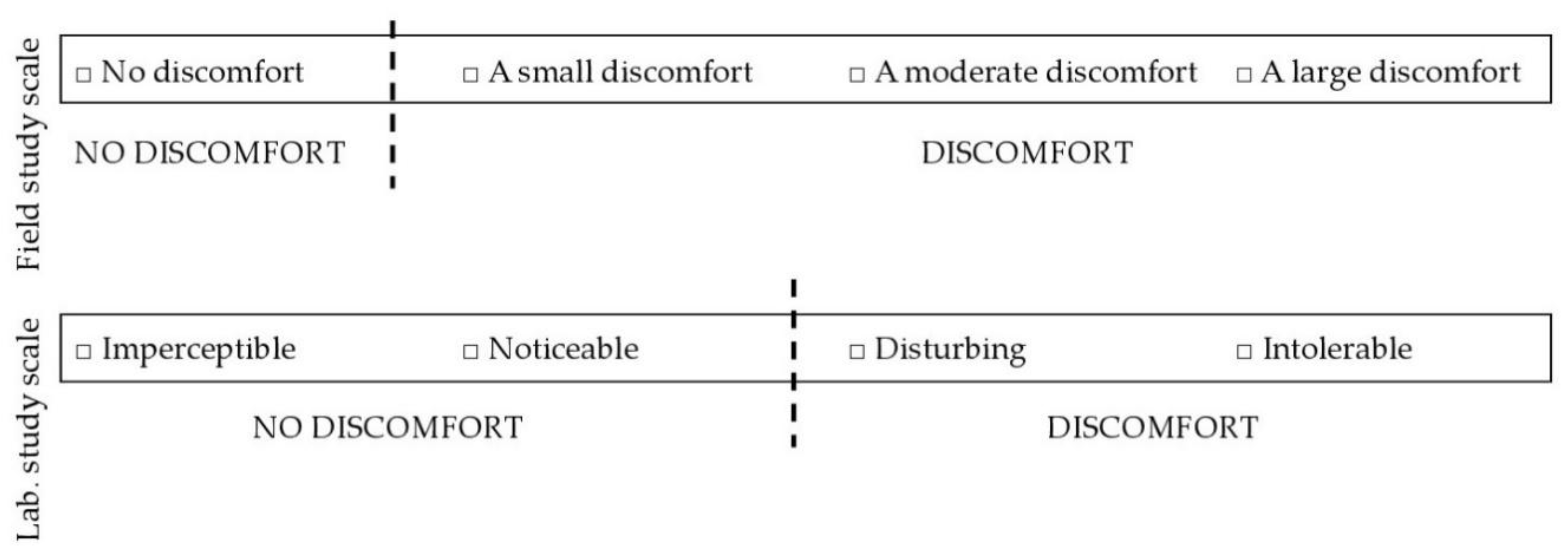
The second statistical approach requires the computation of binary logistic regression models, which use a binary variable as the dependent variable. Therefore, the two 4-point glare scales are first transformed into binary scales: no discomfort-discomfort (Figure 2).
Binary logistic regression models are then computed, with the binary discomfort glare rating as the dependent variable, and each one of the five discomfort glare indices calculated with each one of the 63 evalglare options as the independent variable. The binary logistic regression models estimate the probability that discomfort due to glare is perceived given the value of the explanatory variable, i.e., the discomfort glare index. Bonferroni correction is applied when checking the significance of each logistic regression model.
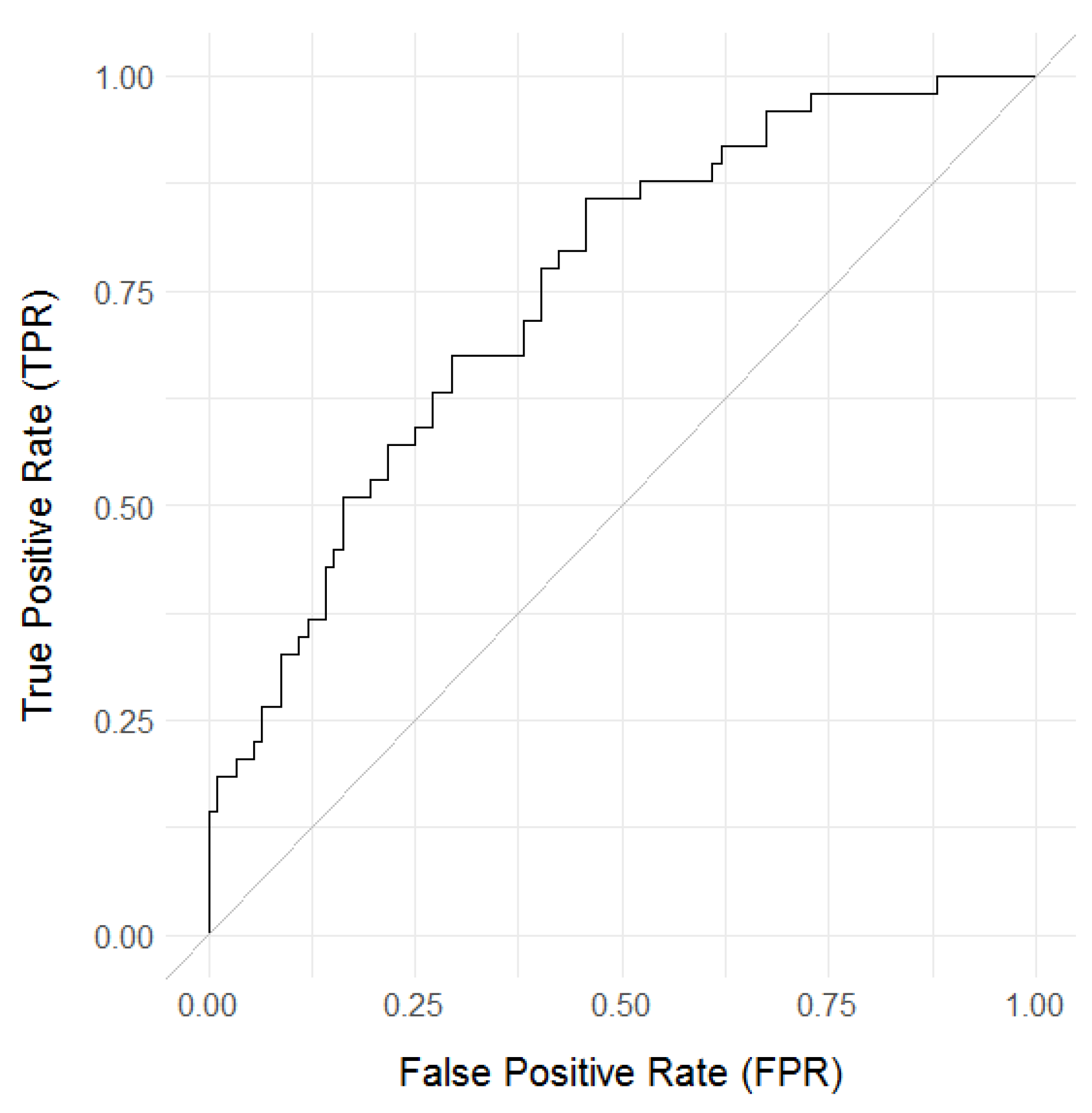
To compare the 63 evalglare options, the Area Under the Receiver Operating Characteristic (ROC) Curve (AUC), specific to each binary logistic regression model, is used. The ROC curve of a logistic regression model illustrates its diagnostic ability for each possible discrimination threshold. In other words, the ROC curve can be plotted in such a way that each point of the curve represents a different cut-off value, and the x and y coordinates of this point correspond, respectively, to the False Positive Rate (FPR) and the True Positive Rate (TPR) of the model when using this cut-off value (Figure 3). The AUC of a logistic regression model is the area comprised beneath the ROC curve of the model. The larger the AUC, the better the model, as the probability of good detection (TPR) is maximized, whereas the probability of false alarm (FPR) is minimized. The AUC of each binary logistic regression model is used as the second indicator of the accuracy of discomfort glare prediction. In the literature, the absolute thresholds for AUC are used to define the quality of discrimination of a model: an AUC < 0.6 corresponds to a failing model, an AUC ≥ 0.6 to a poor model, an AUC ≥ 0.7 to an acceptable model, and an AUC ≥ 0.8 to an excellent model [23,24].
Similarly to the comparison of Spearman correlation coefficients, significance tests can be applied to determine whether the difference between two AUC is statistically significant. Three different significance tests [25,26,27] were applied in this study through the pROC package in R. These tests are designed to compare the AUC of two paired ROC curves, namely ROC curves of logistic regression models built on two variables from the same dataset. Using the same scoring system as for the Spearman indicator, the significance of the difference between each evalglare option resulting from the AUC approach is evaluated on a score going from 0 to 15, since three significance tests are performed for each of the five discomfort glare indices.
3.2.3. Corrected Akaike’s Information Criterion of Ordinal Logistic Regression Models
The last statistical approach involves the computation of ordinal logistic regression models. Ordinal logistic regression models can be interpreted as an extension of the binary logistic regression models, which allows for more than two response categories. These models can therefore be computed directly using a 4-point glare scale as the dependent variable. Instead of estimating the probability that discomfort due to glare will be perceived, the ordinal logistic regression models measure how likely the response is to fall below one of the three thresholds of the 4-point scale, given the value of the independent variable, i.e., the discomfort glare index. Ordinal logistic regression models are computed for each one of the five discomfort glare indices that were calculated with each one of the 63 evalglare options. Bonferroni correction is applied when checking the significance of each model.
By comparing how well the ordinal models fit to the data, the 63 evalglare methods can be compared, so that the evalglare option providing the best accuracy of discomfort glare prediction can be highlighted. One common way of comparing the fit of ordinal logistic regression models is to evaluate their corrected Akaike’s Information Criterion (AICc). The AICc is used as an indicator of the relative information that is lost when a given model is chosen over another model developed on the same dataset. Therefore, the AICc can estimate the relative quality between statistical models computed on the same dataset, but does not give any information about the absolute quality of the model. As a result, AICc thresholds indicating the absolute quality of a model cannot be found in the literature. However, considering each dataset separately, the lower the AICc value, the better the model. The AICc of each ordinal logistic regression model is used as the third and last indicator of the accuracy of discomfort glare prediction to compare the 63 evalglare options.
In contrast to Spearman and AUC statistical approaches, there exists no significance test to statistically compare the AICc of two ordinal logistic regression models. But, several thresholds of the difference between the AICc of two models that were computed from the same dataset have been published in the literature [28,29,30,31]. For this study, a threshold of 10 points, namely a difference of 10 points between the AICc values of two models, was used to determine that the model with the lower AICc value is significantly better than the other one. If the difference between the AICc values of two models that were computed from the same dataset is larger or equal to 10, the significant difference score between these two models is given one point. The significance of the difference between two evalglare options is evaluated on a score from 0 to 5 for each dataset, since the AICc difference test is done for each of the five discomfort glare indices.
4. Results and Discussion
In this section, the results of the study are presented and discussed. First, the three evalglare methods are compared, followed by the comparison of the two background luminance definitions, the three search radius, and the three task area sizes. At last, the use or not of the smooth parameter is investigated as well. Six graphs are used for each comparison: on the left, three graphs related to the field study, and on the right, three graphs related to the laboratory study. From top to bottom, the first graph uses the results of the first statistical approach, namely the Spearman correlation; the second graph uses the results of the second statistical approach, namely the AUC of the binary logistic regression models; and, the third graph uses the results of the third statistical approach, namely the AICc of the ordinal logistic regression models. The statistical results—Spearman correlation and logistic regressions—that were found to be non-significant with Bonferroni correction are still included in the graphs, but they can be recognized by graphical means. The datapoints based on the DGP index were removed from the boxplot graphs. The DGP model is indeed partly based on the vertical illuminance, which does not depend on detected glare sources. These datapoints tend therefore to remain stable throughout the different evalglare options and prevent us from drawing observations from the graphs. However, these datapoints are still plotted in the boxplot graphs as small orange triangle points. Finally, tables summarize for each comparison the total significant difference scores, which are the weighted sum of the significant difference scores of the three statistical approaches (Equation (1)):
with SSD, the total significant difference score;
SSD,Spearman, the significant difference score from the Spearman statistical approach;
SSD,AUC, the significant difference score from the AUC statistical approach; and,
SSD,AICc, the significant difference score from the AICc statistical approach.
4.1. Evalglare Methods
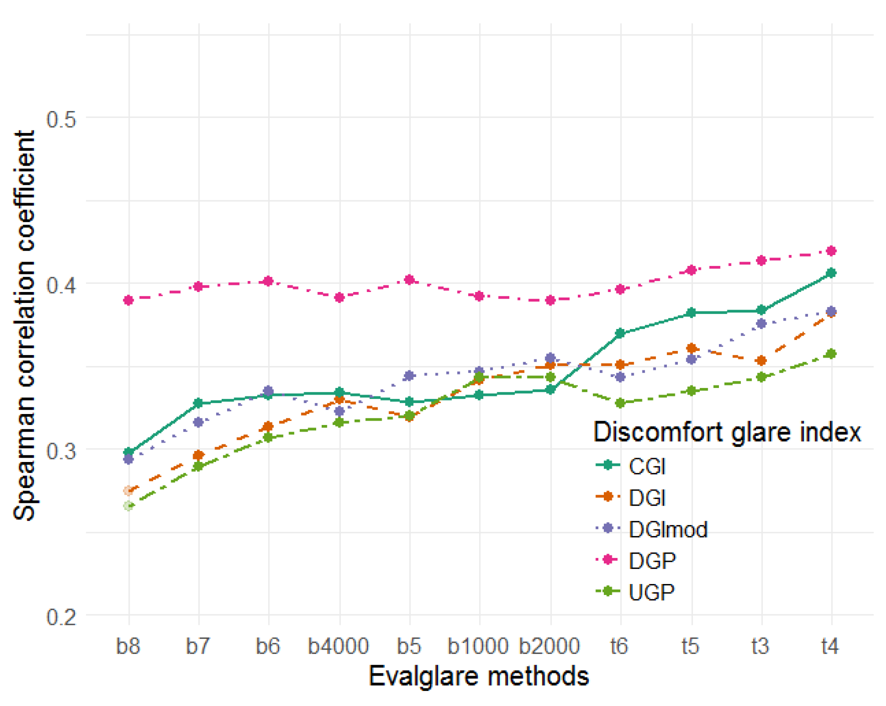
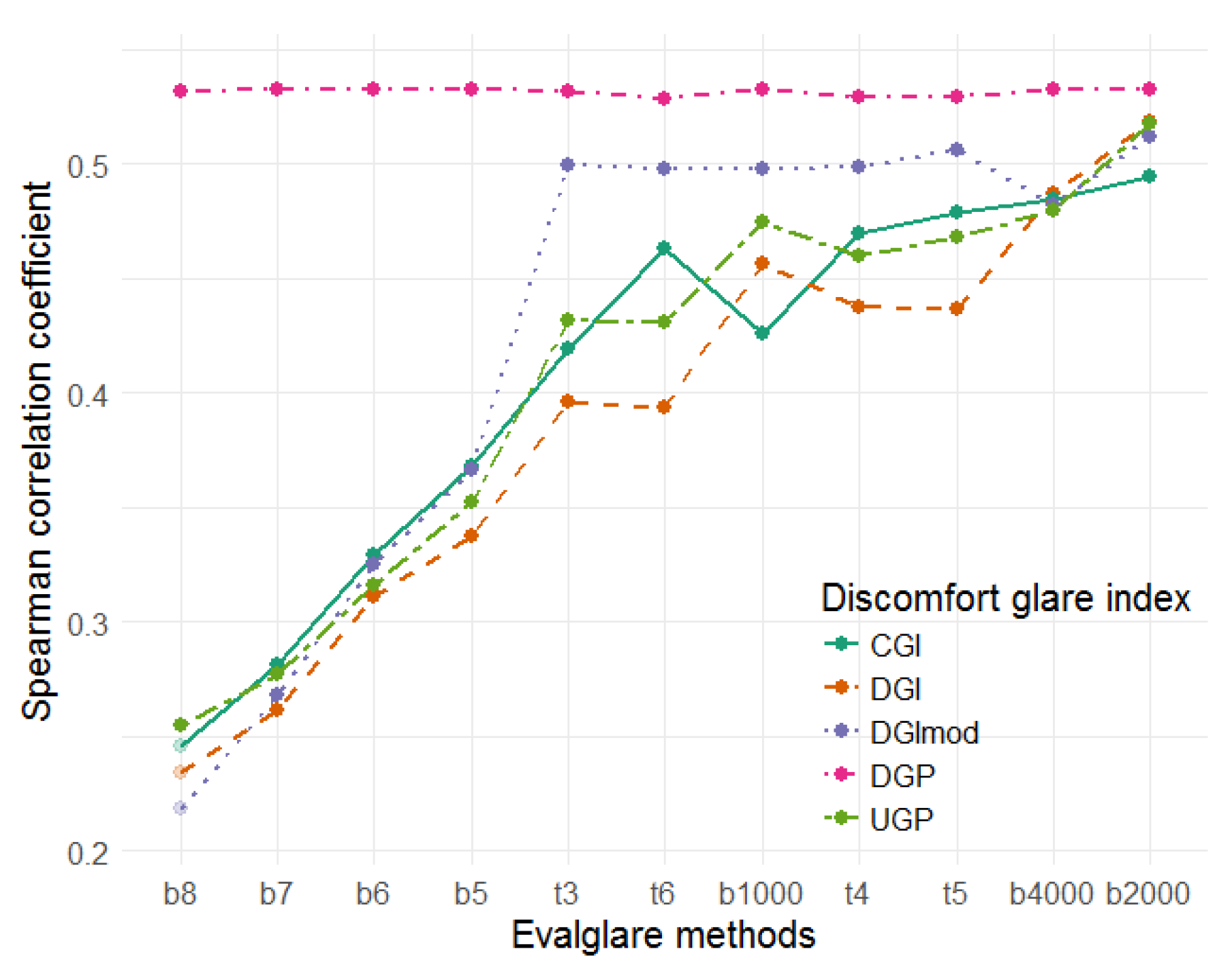
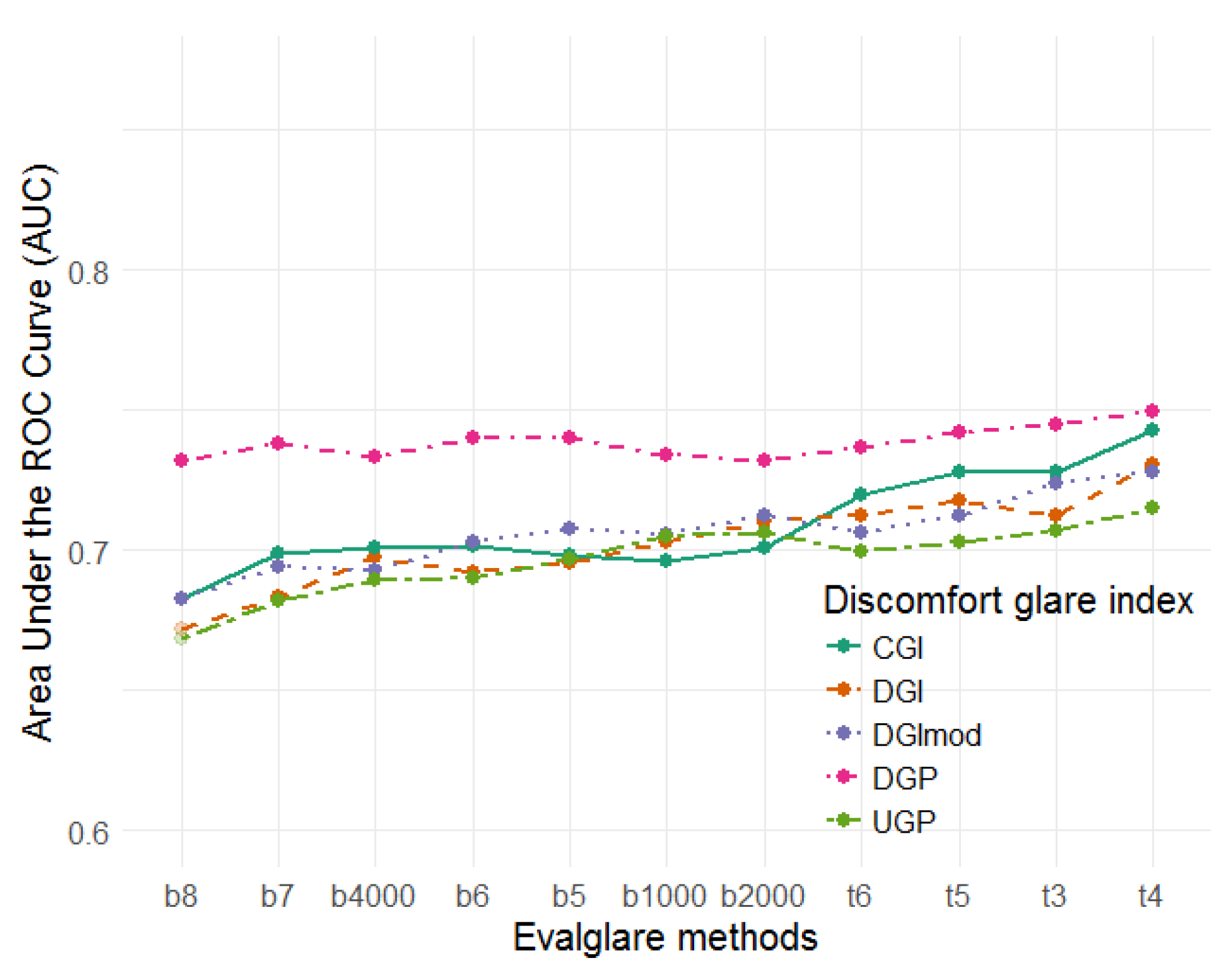
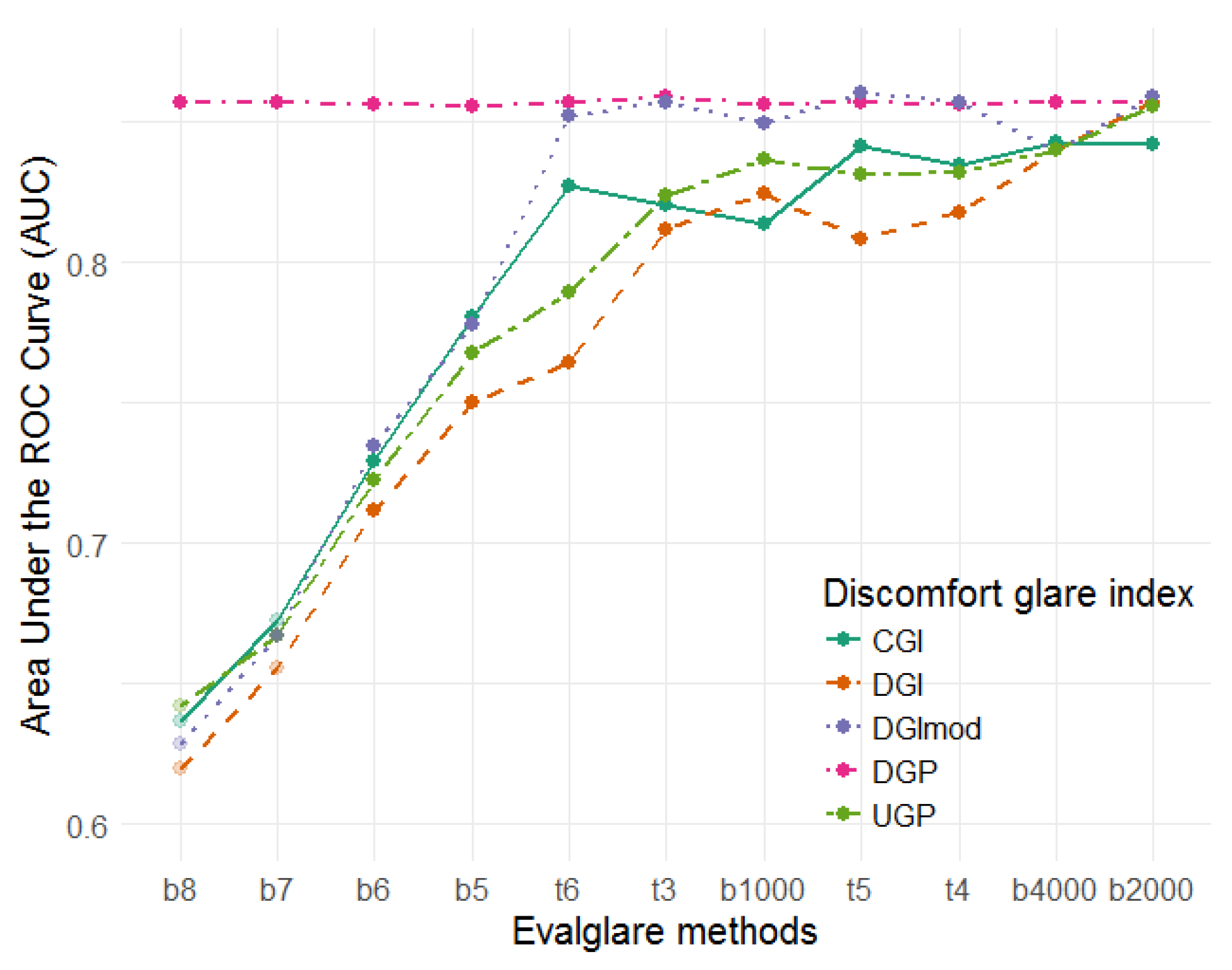
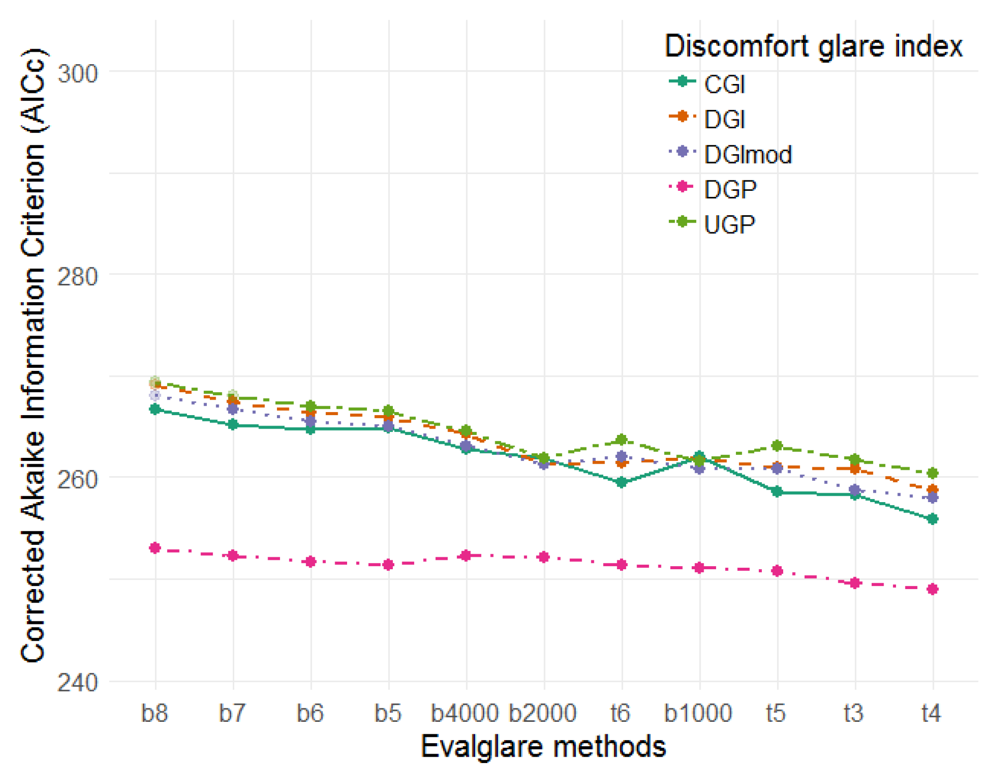
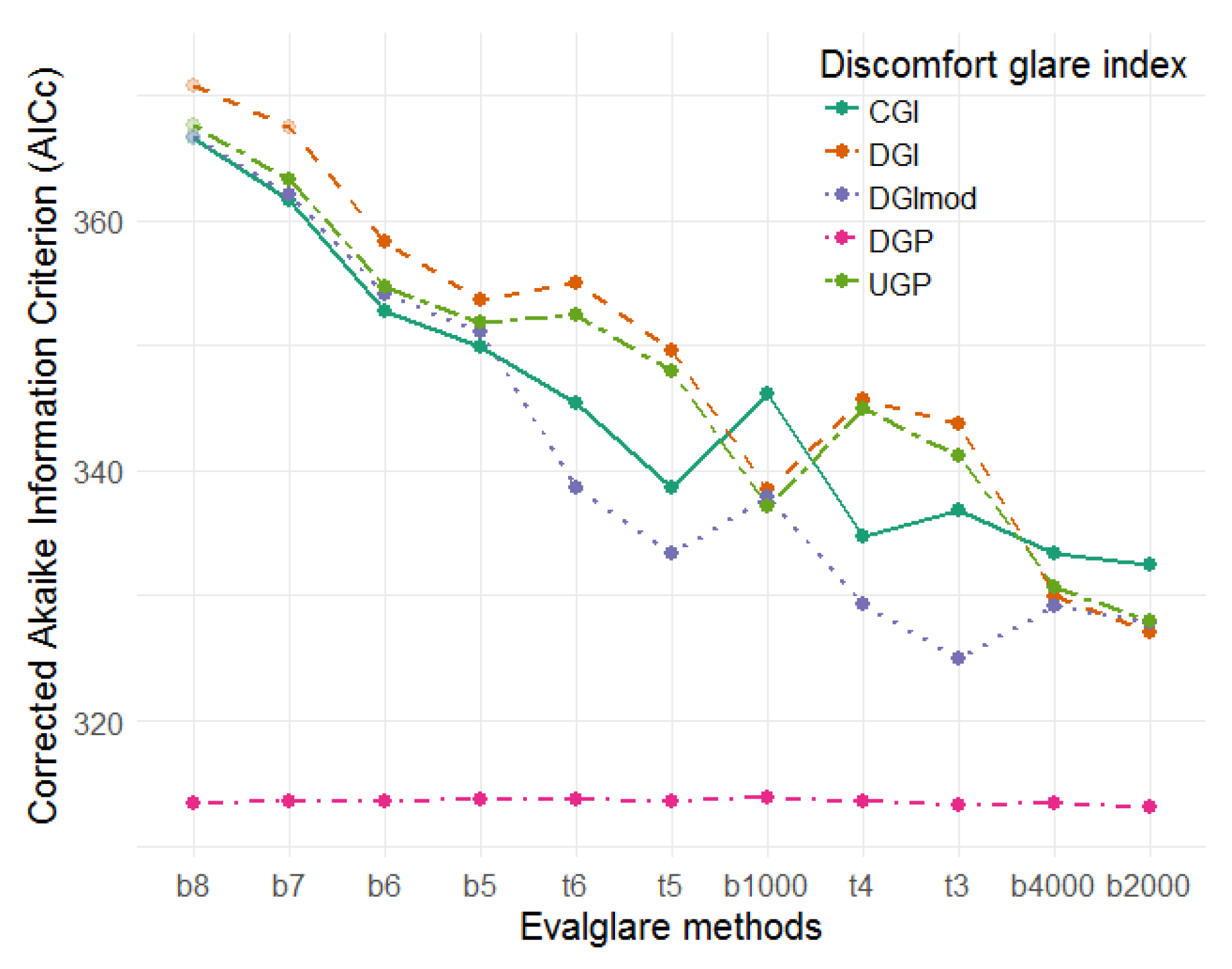
In Figure 4, Figure 5, Figure 6, Figure 7, Figure 8 and Figure 9, the indicators of accuracy of discomfort glare prediction are compared between the 11 different evalglare methods used in this study—factor method with factor 5, 6, 7, and 8; threshold method with threshold 1000, 2000, and 4000; task area method with factor 3, 4, 5, and 6. All other parameters (background luminance definition, search radius, task area size, and smooth option) are set to their default value, so that the methods can be compared on a neutral basis. This comparison is done for each of the five discomfort glare indices (DGP, DGI, CGI, DGImod, UGP), and for both the field (left) and laboratory (right) studies. Non-significant statistics (Spearman correlation and logistic regressions) are included in the graphs but are plotted as dimmed dots. The methods are classified along the X-axis in an ascending order of performance, in such a way that the best performing method can be easily recognized on the right.
From the graphs (Figure 4, Figure 5, Figure 6, Figure 7, Figure 8 and Figure 9), it appears that the task area method seems to be more appropriate for the field study, and the threshold method for the laboratory study. The task area used with a factor 4 (t4) and the threshold of 2000 cd/m2 (b2000) are the methods providing the best accuracy of discomfort glare prediction throughout the three different statistical approaches. In the graphs, the non-significant statistics—Spearman correlation coefficients or logistic regression models—are identifiable as the transparent points. Only a few appear to be non-significant, and these are only found in the factor method. For both studies, the factor methods (b5, b6, b7, b8) are the ones that are producing the worst discomfort glare prediction. In addition, the differences between the methods are more pronounced for the laboratory study than for the field study. This is probably partly due to the noise inherent to field studies data.
As observed in Table 4 and Table 5, the significant difference scores do not exceed 82%. This is due to the fact that the difference between two evalglare options used to derive the DGP will almost never be large and significant, since this index was designed to be robust against variations of glare source detection methods. Therefore, a score of 80% means that for all other discomfort glare indices and for each significance test applied, the difference between the evalglare methods were significant. As already observed from the graphs, the differences are larger in the case of the laboratory study. The scores of the laboratory study support the hypothesis that the differences between the factor methods and the other methods are statistically significant, with the discomfort glare prediction becoming worse as the factor of the factor method is increased.
From these results, it is clear that the factor methods should be avoided. These methods provide inappropriate glare source detections, which result in inaccurate discomfort glare predictions. Why these methods fail to accurately detect glare sources could be answered by the following explanation.
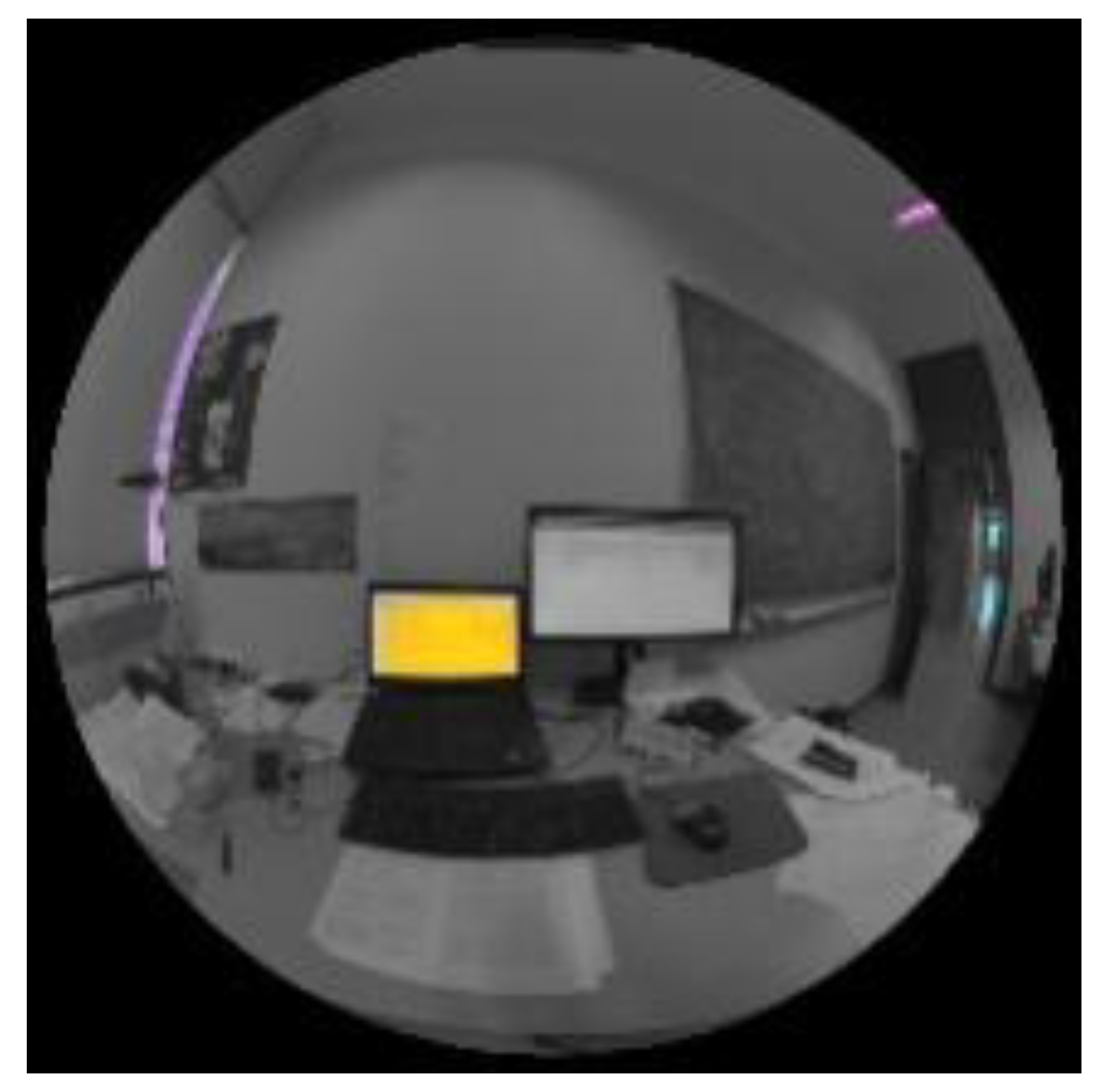
For dim light scenes, the glare source detection threshold while using a factor method will be generally quite low, since the average luminance of the scene is low. This will often result in an over-detection of glare sources. Figure 10 shows an example of a visual scene in which the computer screen was treated as a glare source by evalglare and factor 5 method, although the visual scene was ranked as “No discomfort” by the subject.
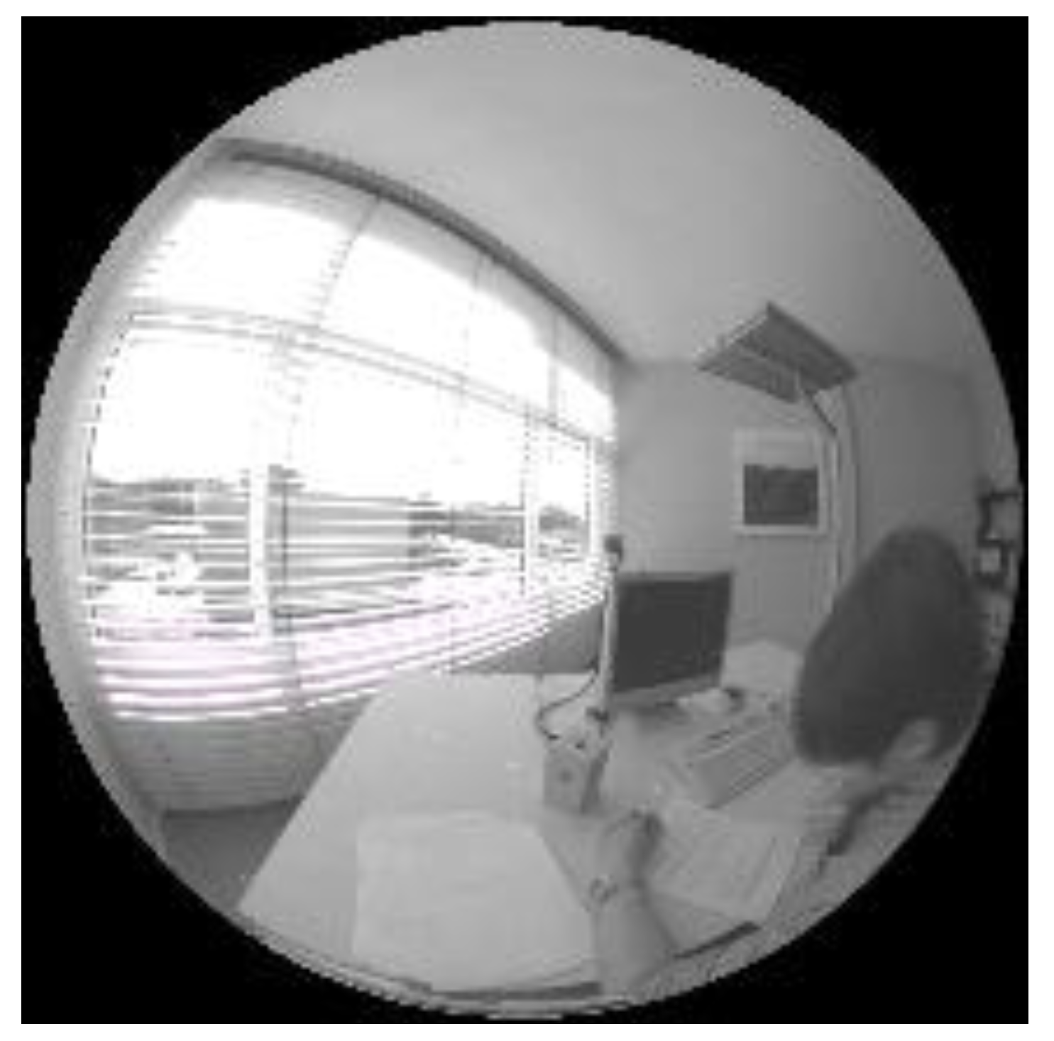
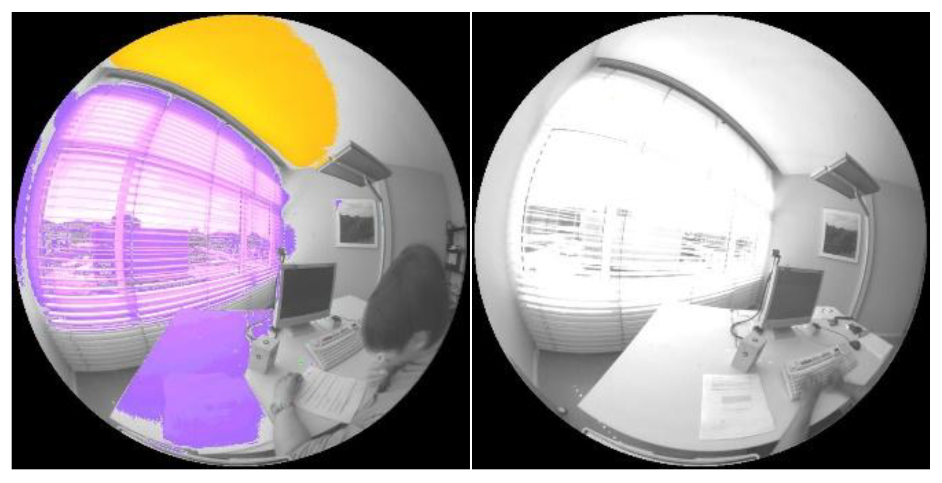
On the opposite, when a scene is bright, the factor method will often fail to find glare sources (under-detection). Since the average luminance of the scene is relatively high, the glare source detection threshold will be high as well. Evalglare will thus miss some glare sources. The visual scene in Figure 11 was rated as “Disturbing”, although no substantial glare sources were detected by evaglare and factor 7 method.
From the results, it can also be inferred that the choice of an evalglare method can be done according to the type of discomfort glare that is the most probable to occur in the studied visual scene. It appears that the task area method would be the most appropriate for visual scenes, in which contrast glare is likely to occur. On the other hand, the threshold method offers some advantages when being used for visual scenes with saturation glare, although the task area method delivers results in a similar range. This observation was expected and can be explained.
In the case of contrast glare, i.e., in the case of low vertical illuminance scenes, like in the field study, the task area method would be more appropriate since the adaptation level of the subject’s eyes plays an important role in the determination of the glare source luminance level at which glare is perceived. The task area method includes the adaptation level in the glare source detection process, by using a task area as reference for the eyes adaptation level.
On the other hand, for saturation glare, which occurs in scenes with relatively high vertical illuminance, like in the laboratory study, the determination of the glare source luminance threshold does not directly depend on the adaptation of the subject’s eyes. Therefore, an absolute threshold would offer better results for saturation glare detection. Up to now, the most common threshold value has been 2000 cd/m2, and this value is supported by this study.
4.2. Background Luminance Definition
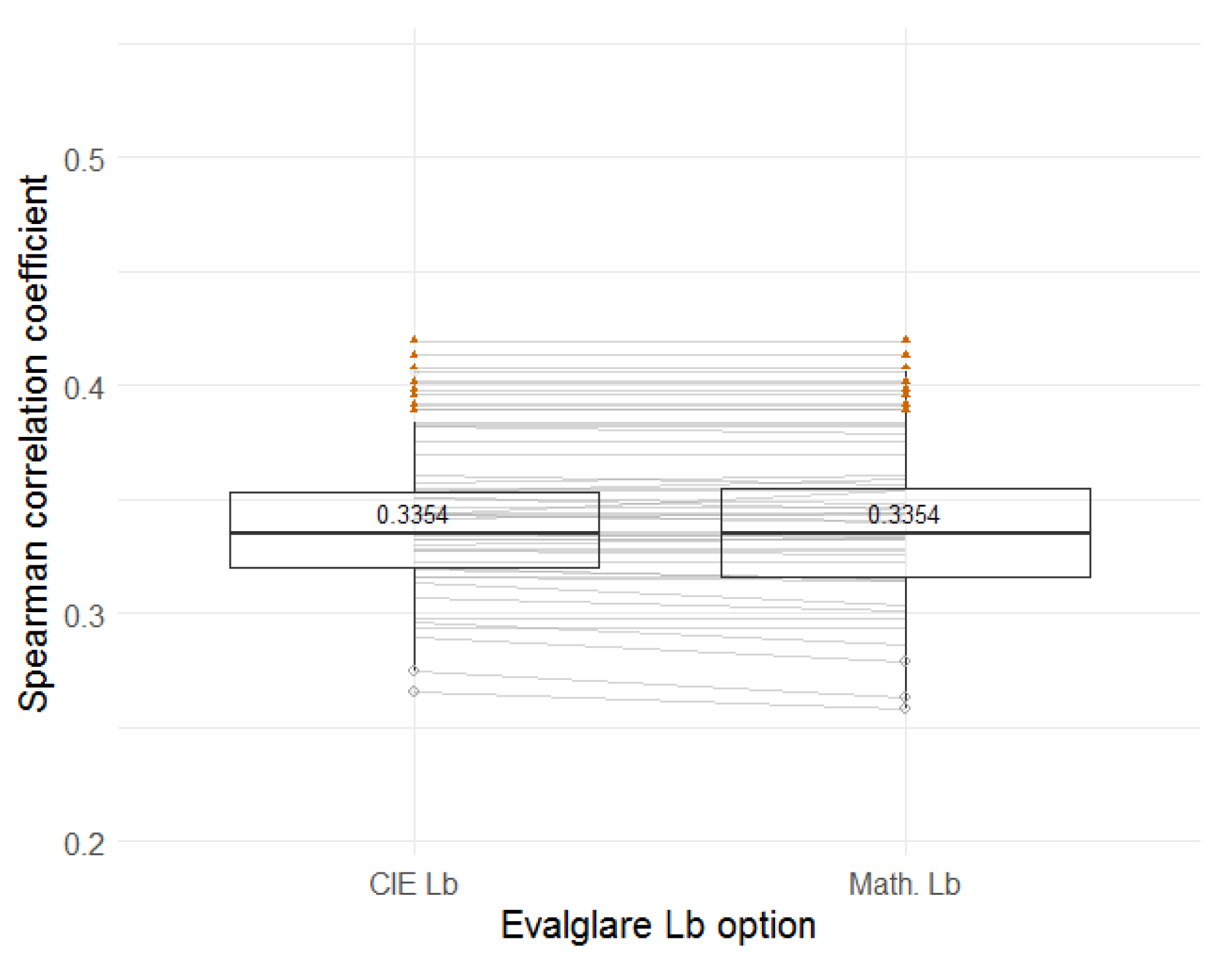
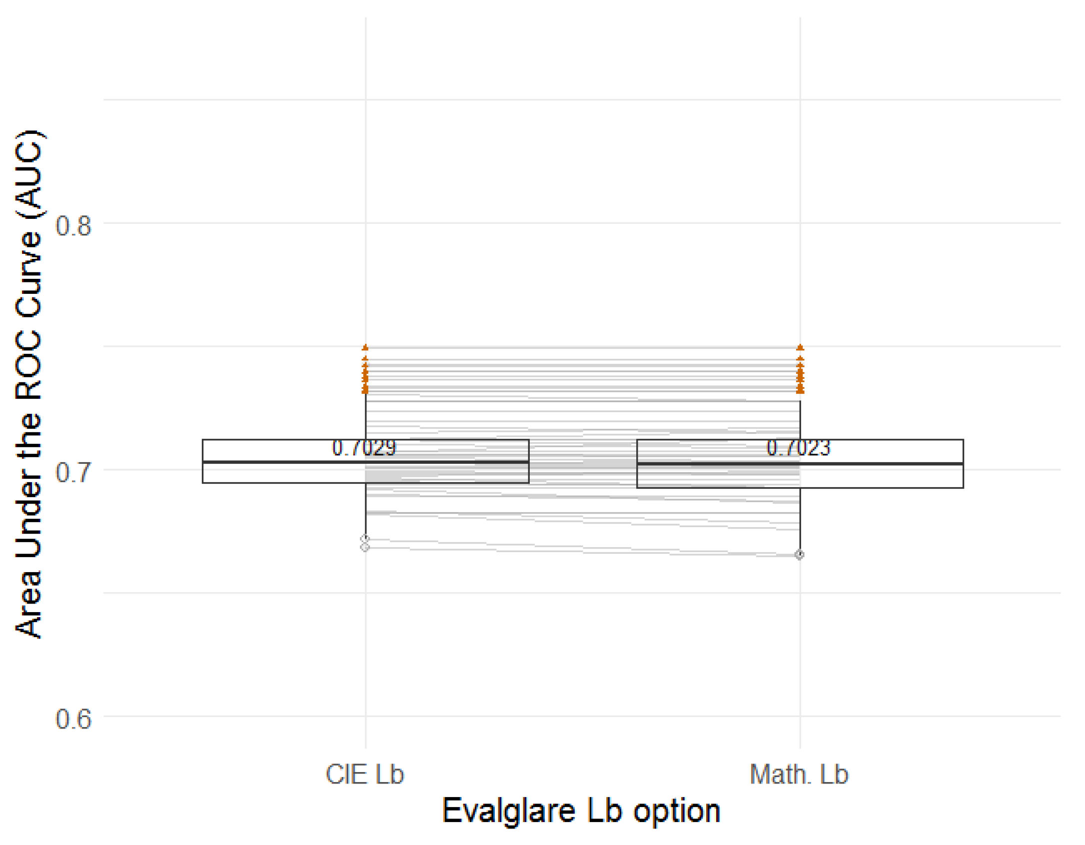
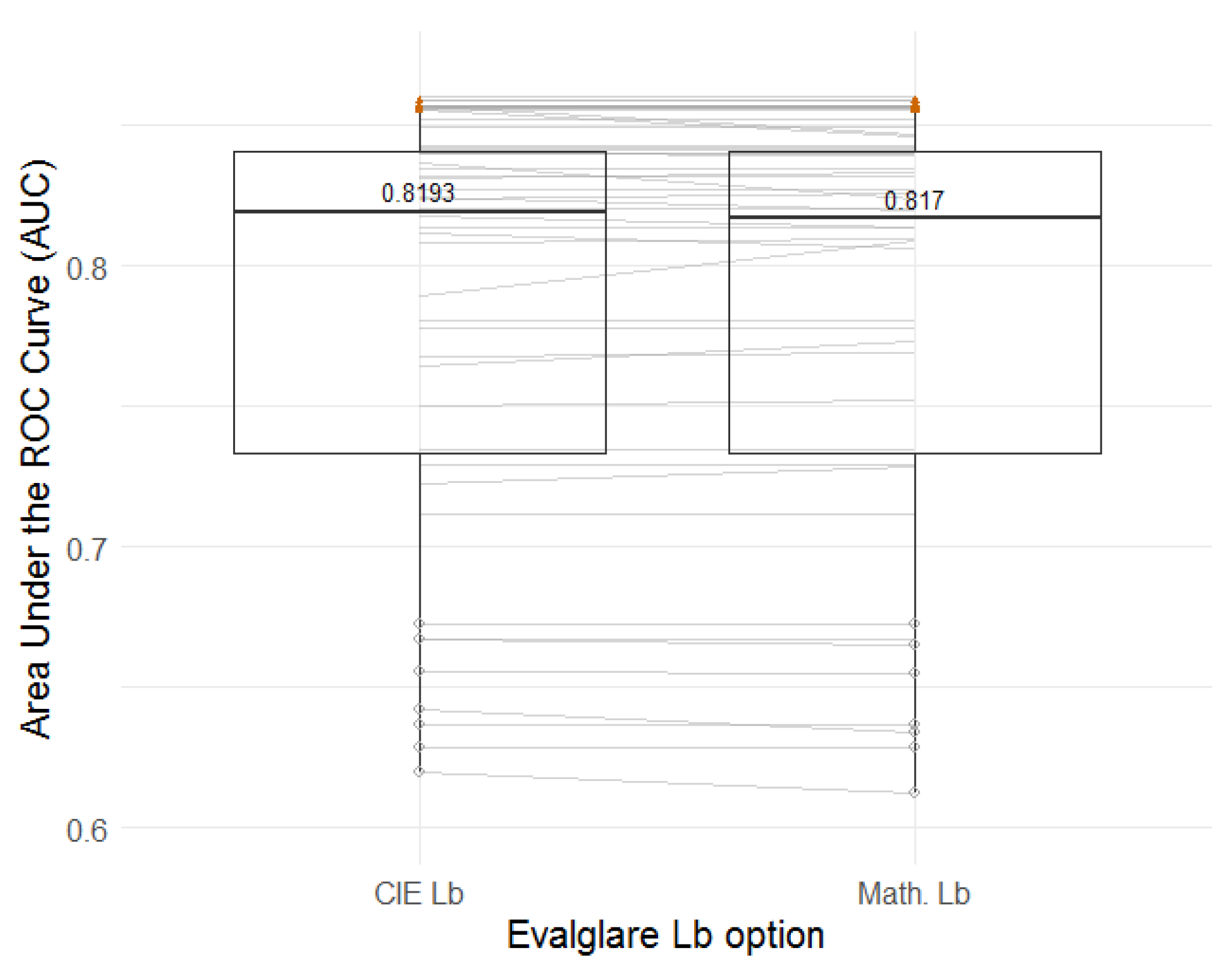
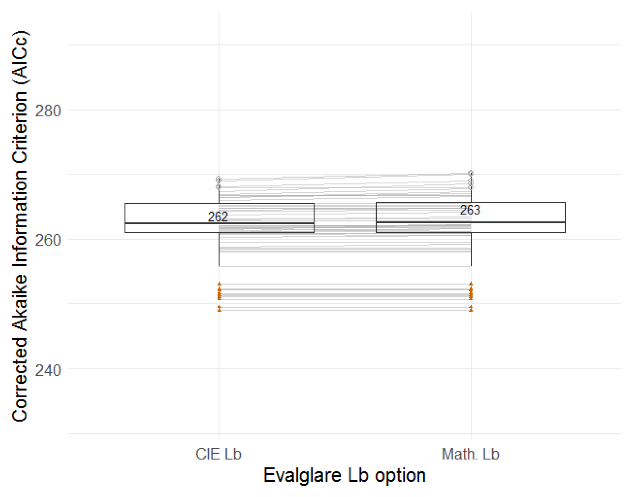
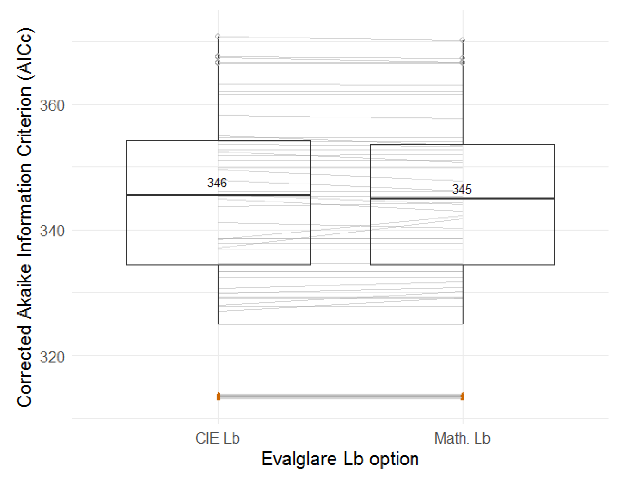
Figure 12, Figure 13, Figure 14, Figure 15, Figure 16 and Figure 17 compare the two background luminance definitions by using boxplots for both the field (left) and laboratory (right) studies, of the three indicators of accuracy of discomfort glare prediction. More specifically, each boxplot is based on a group of 44 datapoints, with each one being an indicator corresponding to one of the four discomfort glare indices (DGP is left out of the boxplots) and one of the 11 evalglare methods (b5, b6, b7, b8, b1000, b2000, b4000, t3, t4, t5, t6). Non-significant statistics (Spearman correlation and logistic regressions) are included in the boxplots but are plotted as empty grey dots. The orange triangle points represent the indicators based on the DGP index. At last, the lines connecting two adjacent boxplots represent the evolution of an indicator when the background luminance definition is varied. If the lines would cross each other, then the influence of the background luminance definition would depend on the evalglare method or on the discomfort glare index used. Since the lines are not crossing much in this case, the influence of the background luminance definition is constant, whatever the evalglare method or the discomfort glare index is.
In each figure (Figure 12, Figure 13, Figure 14, Figure 15, Figure 16 and Figure 17), the overall accuracy of discomfort glare prediction can be compared between the use of the CIE definition of the background luminance and its mathematical definition. The difference between the two background luminance definitions lies in the fact that the CIE definition takes into account the cosine correction (Lambert’s cosine law) in the computation of the background luminance. But, it seems that this difference does not show in the accuracy of discomfort glare prediction: the boxplots are similar for the field and laboratory studies and for each statistical approach. On another note, the boxplots of the laboratory study are more spread than those of the field study. Therefore, the variation in the accuracy of discomfort glare prediction between the evalglare methods or between the discomfort glare indices are larger for the laboratory study, as it was already observed in Figure 4, Figure 5, Figure 6, Figure 7, Figure 8 and Figure 9.
Significance tests looking at the difference between the two background luminance definitions support the observations that are made according to the boxplots. The significant difference scores (Table 6 and Table 7) do not exceed 13%, and are mainly 0%. This illustrates that the difference between the two definitions is almost never significant, depending on which significance test is applied. This is confirmed by looking more closely to the boxplots that are related to the AICc indicator: the variation in the AICc values between the use of the CIE definition or the mathematical definition is never larger than 10 points.
From these observations, it appears that there is no significant difference in the accuracy of discomfort glare prediction between the use of the CIE definition and the mathematical definition of the background luminance. Both could be used alternatively without observing any change in the results of a study. However, the influence of the background luminance definition, namely the influence of the use of the cosine correction in the background luminance computation, should be checked in the case of extreme visual scenes. Indeed, this parameter could have an influence when the luminance distribution of the background of a visual scene is extremely heterogeneous, for instance, when background luminance values are much higher—but is still not considered as a glare source—in one specific part of the field of view.
4.3. Search Radius
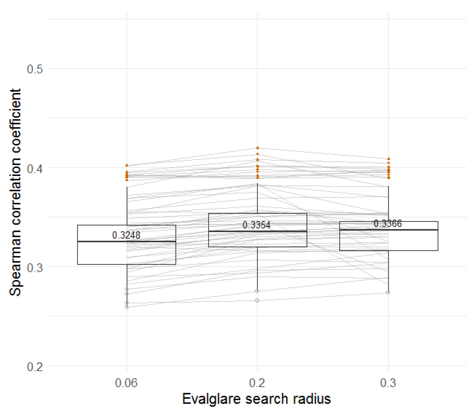
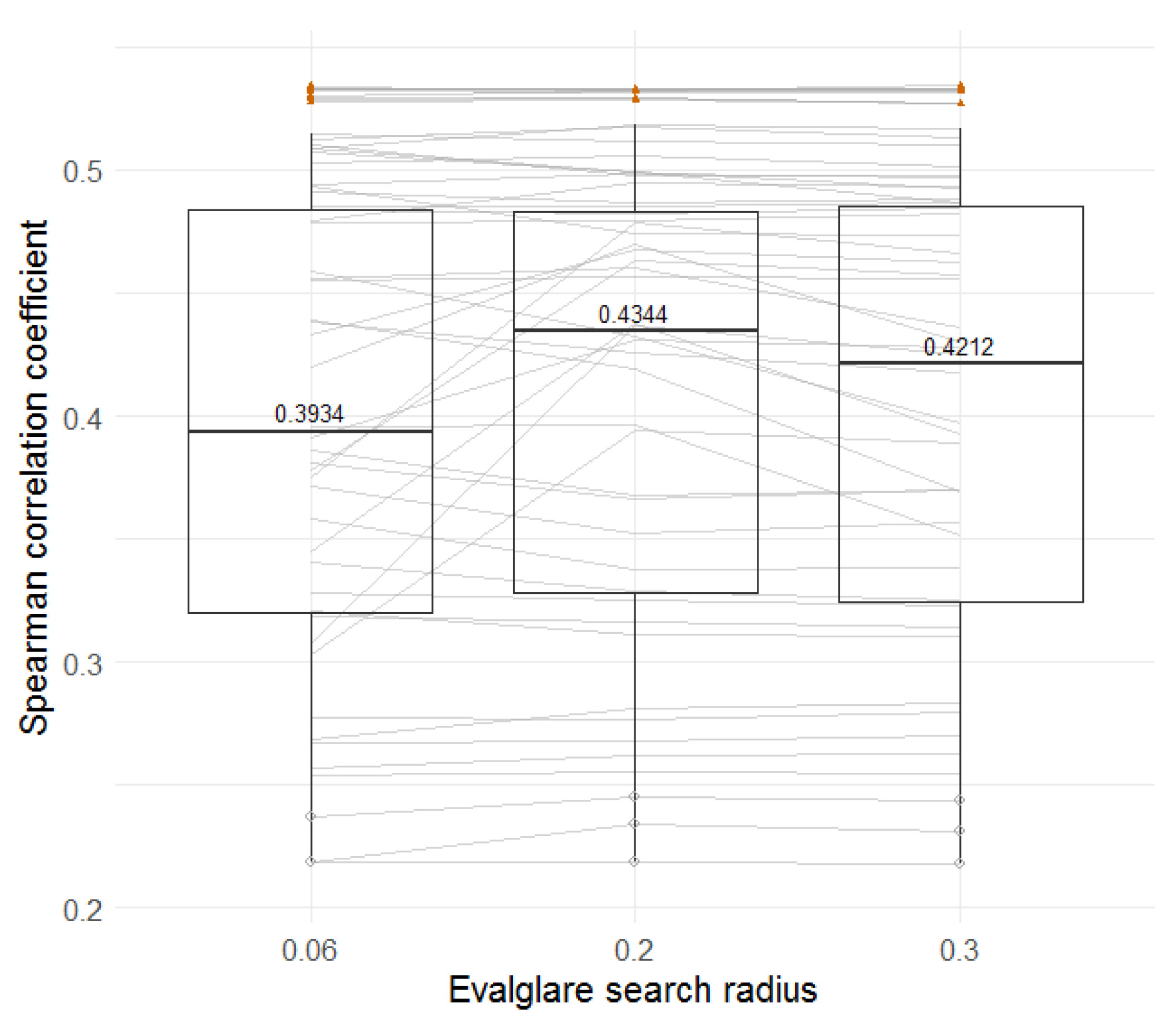
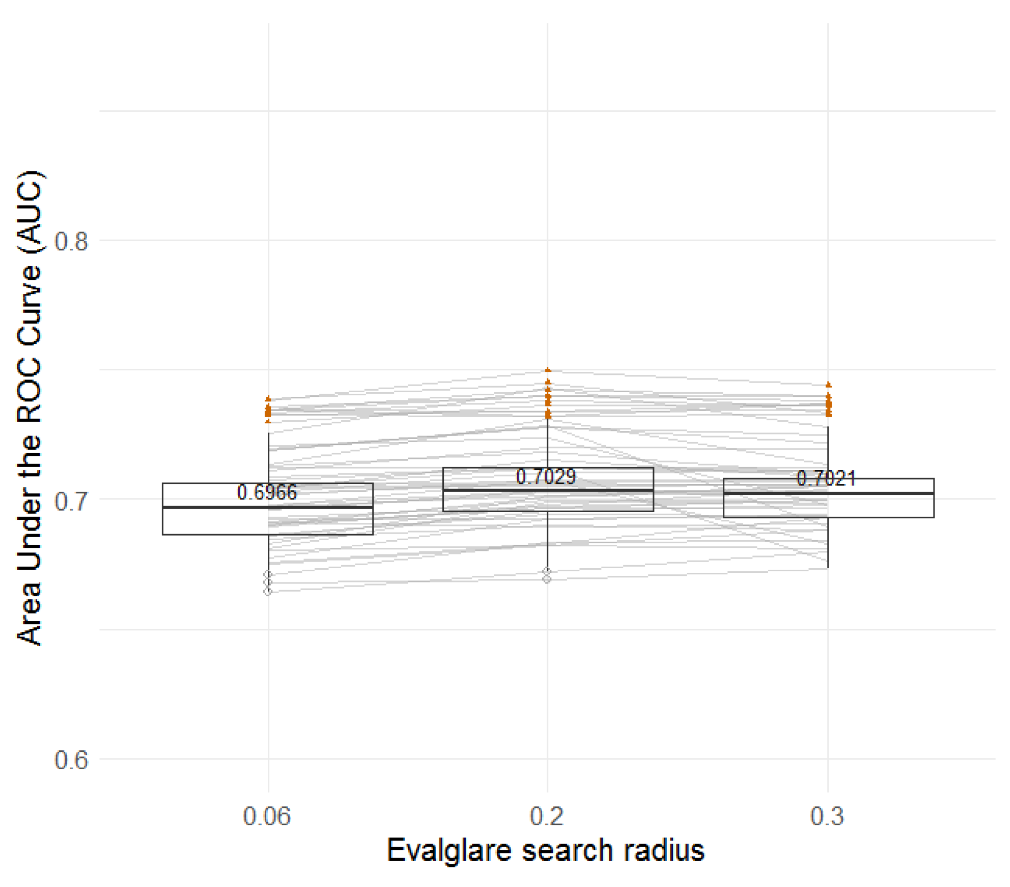
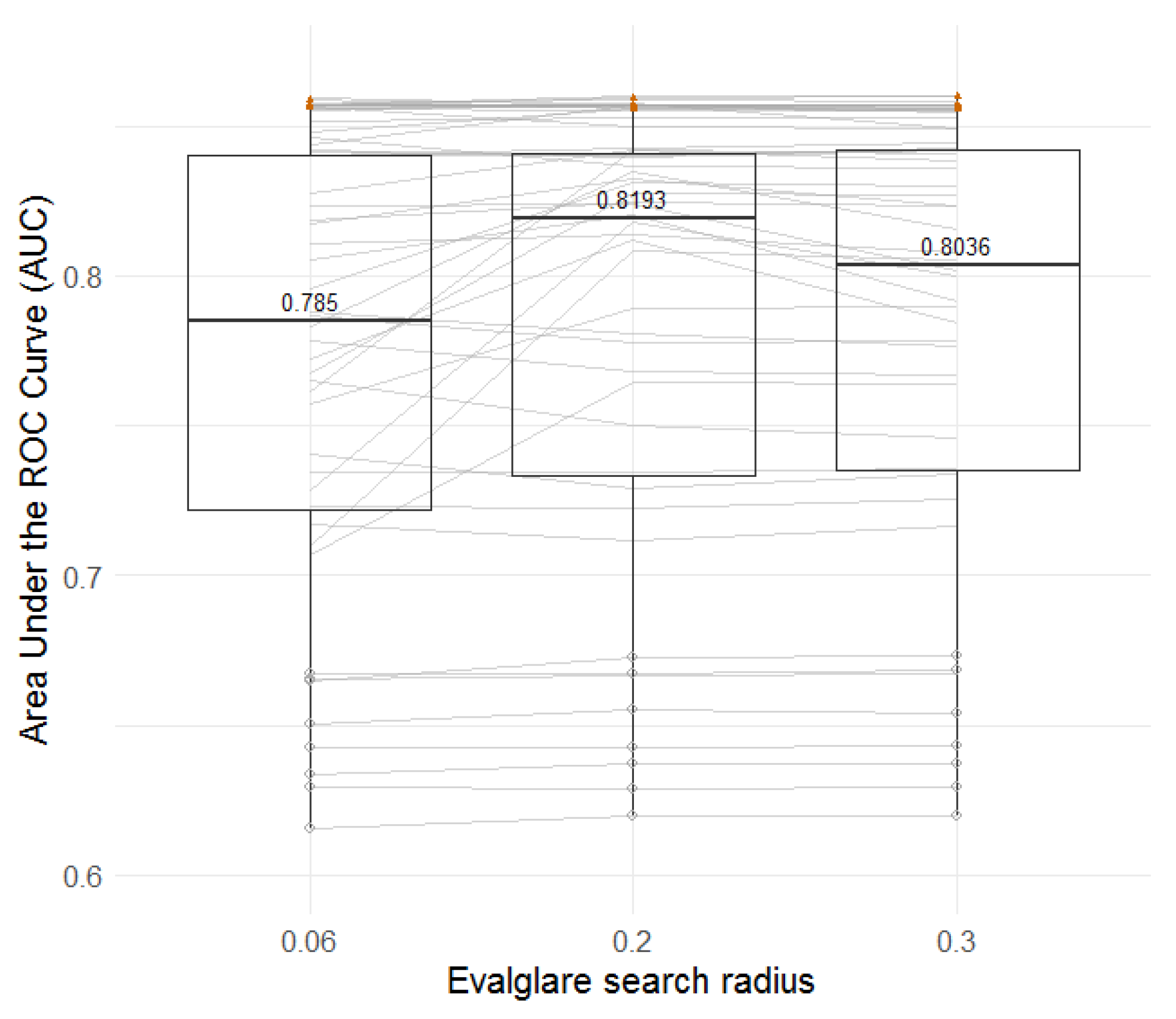
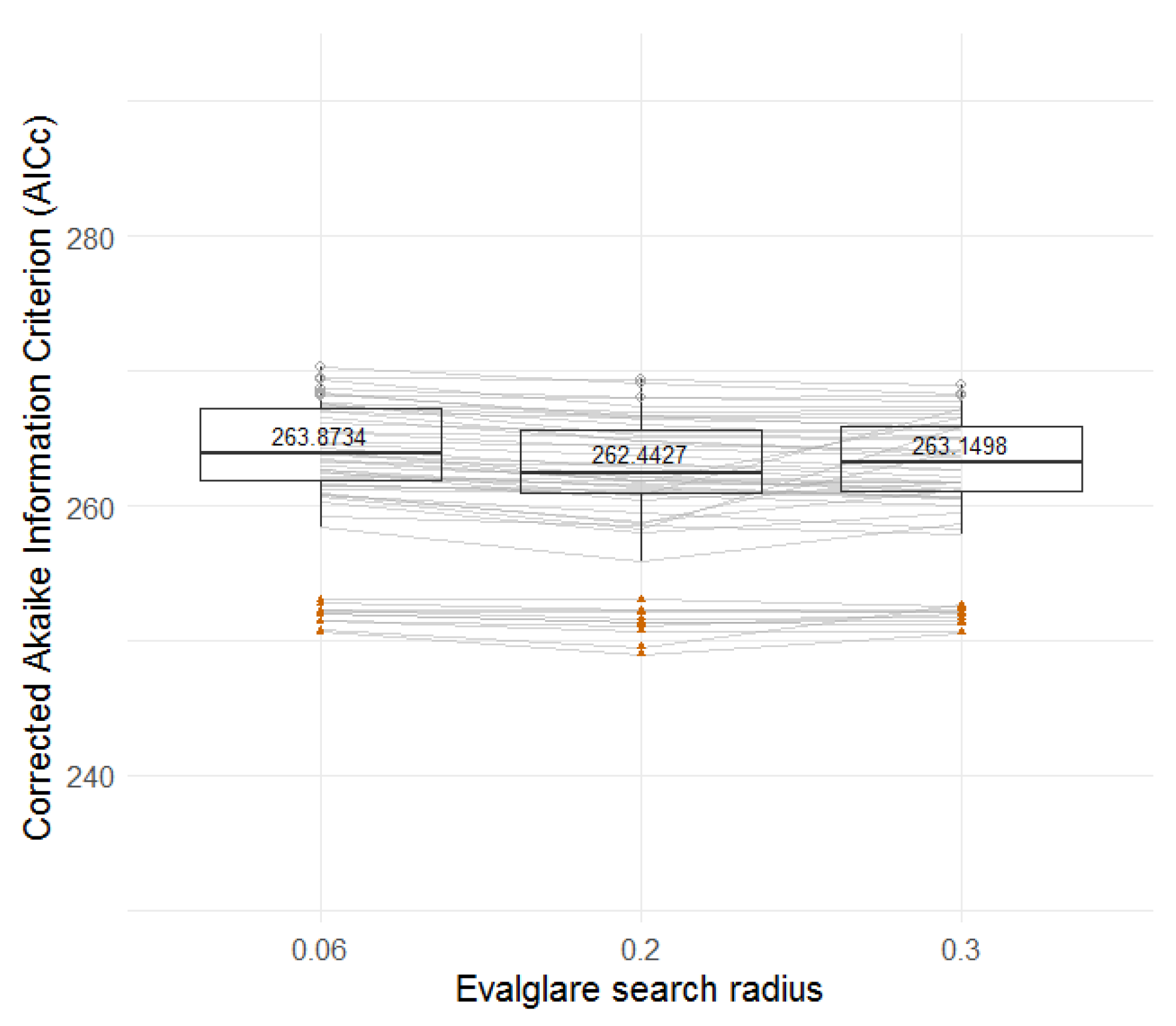
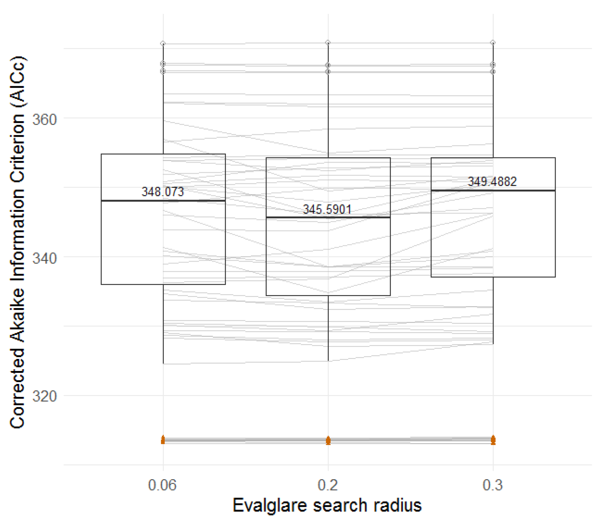
Figure 18, Figure 19, Figure 20, Figure 21, Figure 22 and Figure 23 show boxplots that are built on the same principals than those in Figure 12, Figure 13, Figure 14, Figure 15, Figure 16 and Figure 17, but in this case, the evalglare parameter being varied is the search radius. In each figure (Figure 18, Figure 19, Figure 20, Figure 21, Figure 22 and Figure 23), the overall accuracy of discomfort glare prediction can be compared between the use of a search radius having an opening angle of 0.06, 0.2, or 0.3 radians. By varying the search radius, the maximal distance within which two nearby glaring pixels are merged in one glare source is varied. Therefore, the smaller the search radius, the smaller the solid angle of the detected glare sources but the more of them.
The default search radius in evalglare is 0.2 radians, and it appears from the boxplots that this default parameter is appropriate. It is the one providing the best accuracy of discomfort glare prediction in the field and laboratory studies. However, several lines are crossing, especially in the laboratory study, as some lines go up while others go down when varying the search radius. This is a sign that the influence of the search radius is not constant.
Looking at the significant difference scores between the three search radius parameters (Table 8 and Table 9), it appears that this parameter does not produce significant differences on the accuracy of discomfort glare prediction, at least not for the factor and threshold methods. When using the task area method, the differences might be interpreted as statistically significant in some cases. These cases correspond to the lines with the steepest slopes in the boxplot graphs.
Although the differences in the accuracy of glare prediction could not be demonstrated as being significant in a majority of cases, there seems to be a tendency towards a better accuracy of discomfort glare prediction when using the default search radius. However, using only three variations of the search radius is not enough to grasp the full extent of the influence of the search radius on glare source detection, and indirectly on the accuracy of discomfort glare prediction. Moreover, the influence of the search radius most probably depends on the visual scene, and especially on the distance between two contrasted glare pixels in a luminance map. In the case of this study, the observers from both datasets were sitting close to the façade, thus at a relatively close distance from the blinds. But, this might not be the case for large open-plan offices. If the observer is located further away from the blinds, the distance between the contrasted pixels of the blinds will vary in the luminance map, and the opening angle of the search radius will have to be varied in order to produce a similar result than if the observer was sitting close to the façade. An extended study on the appropriate search radius for glare source detection would be required to thoroughly understand the influence of this parameter. In the meantime, it seems reasonable to keep using the default evalglare search radius having an opening angle of 0.2 radians.
4.4. Task Area Size
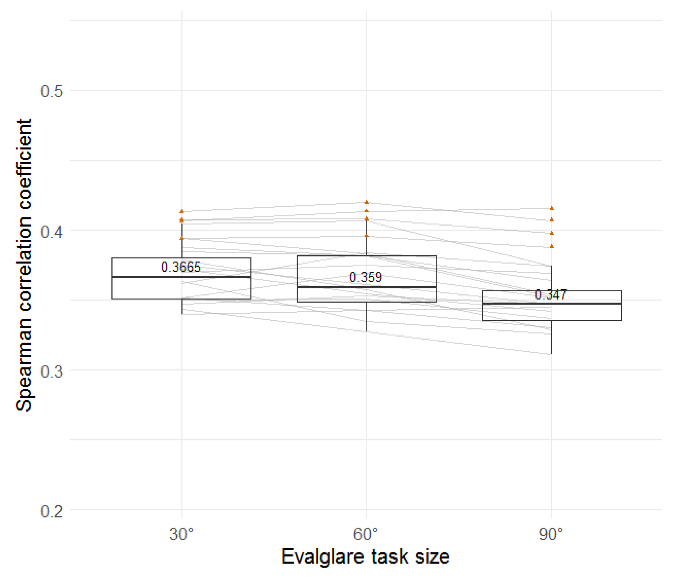
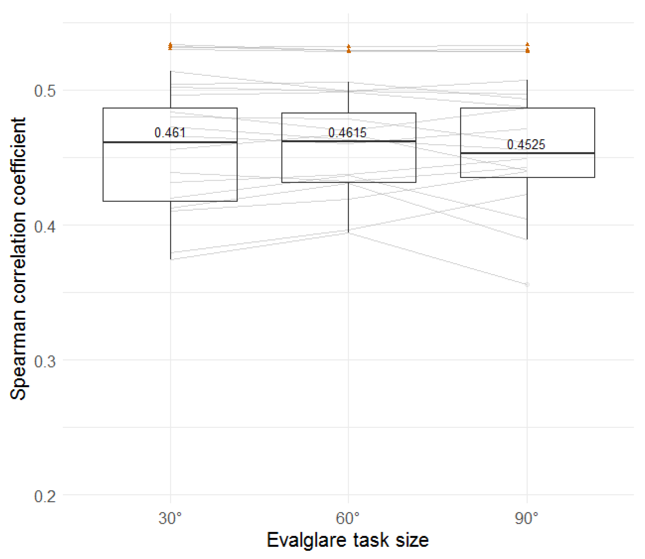
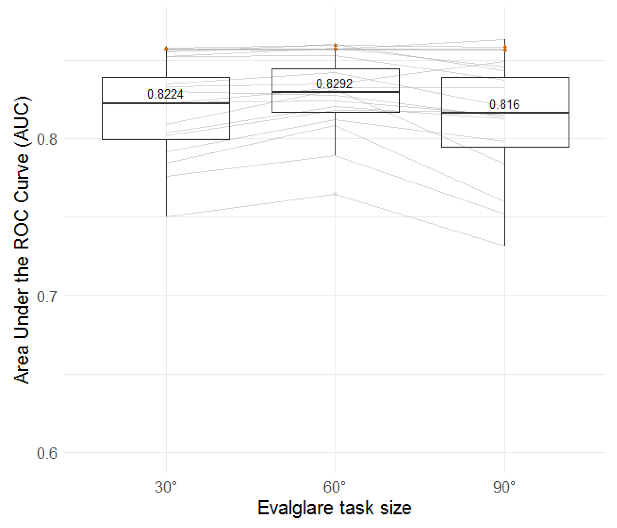
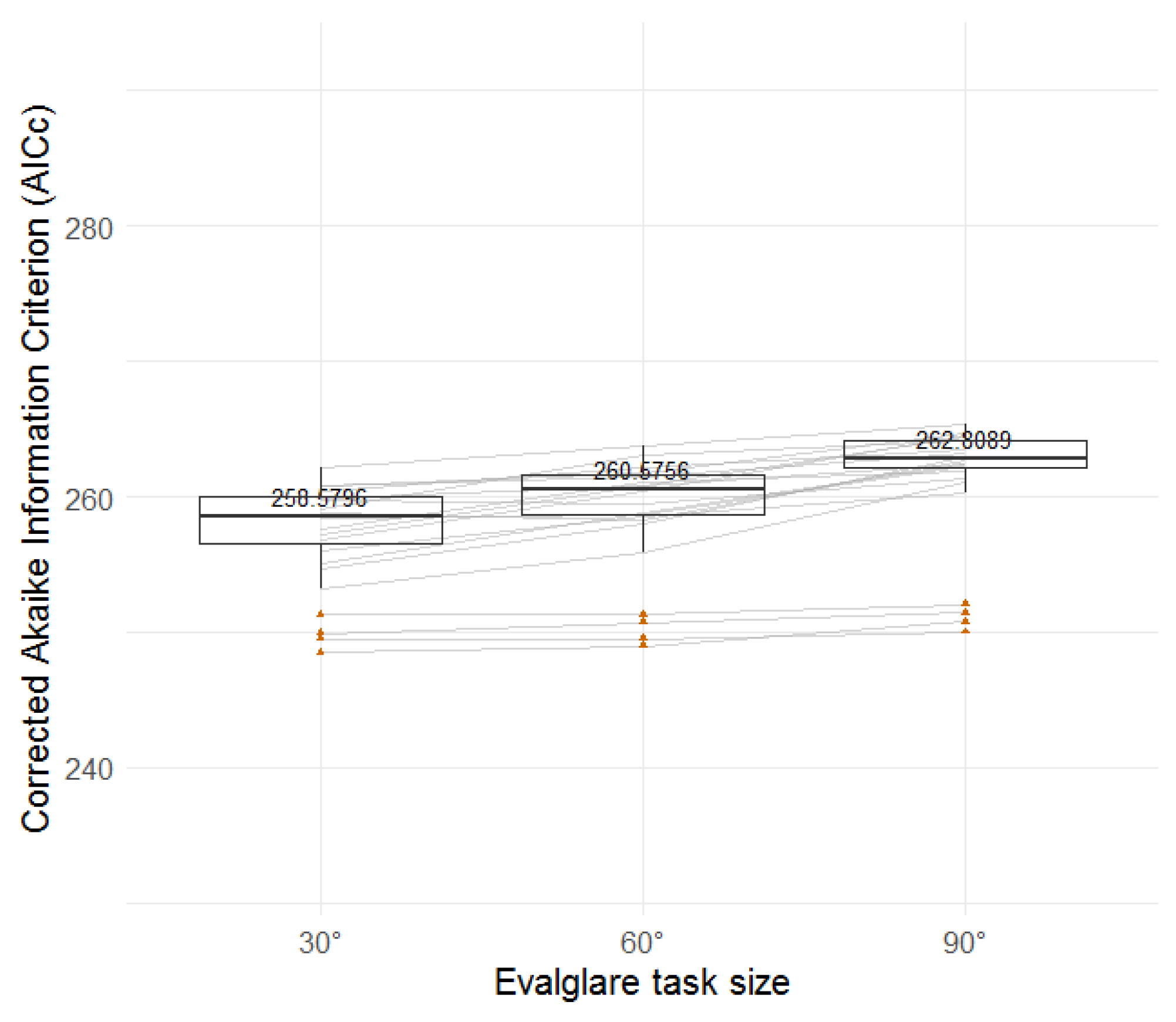
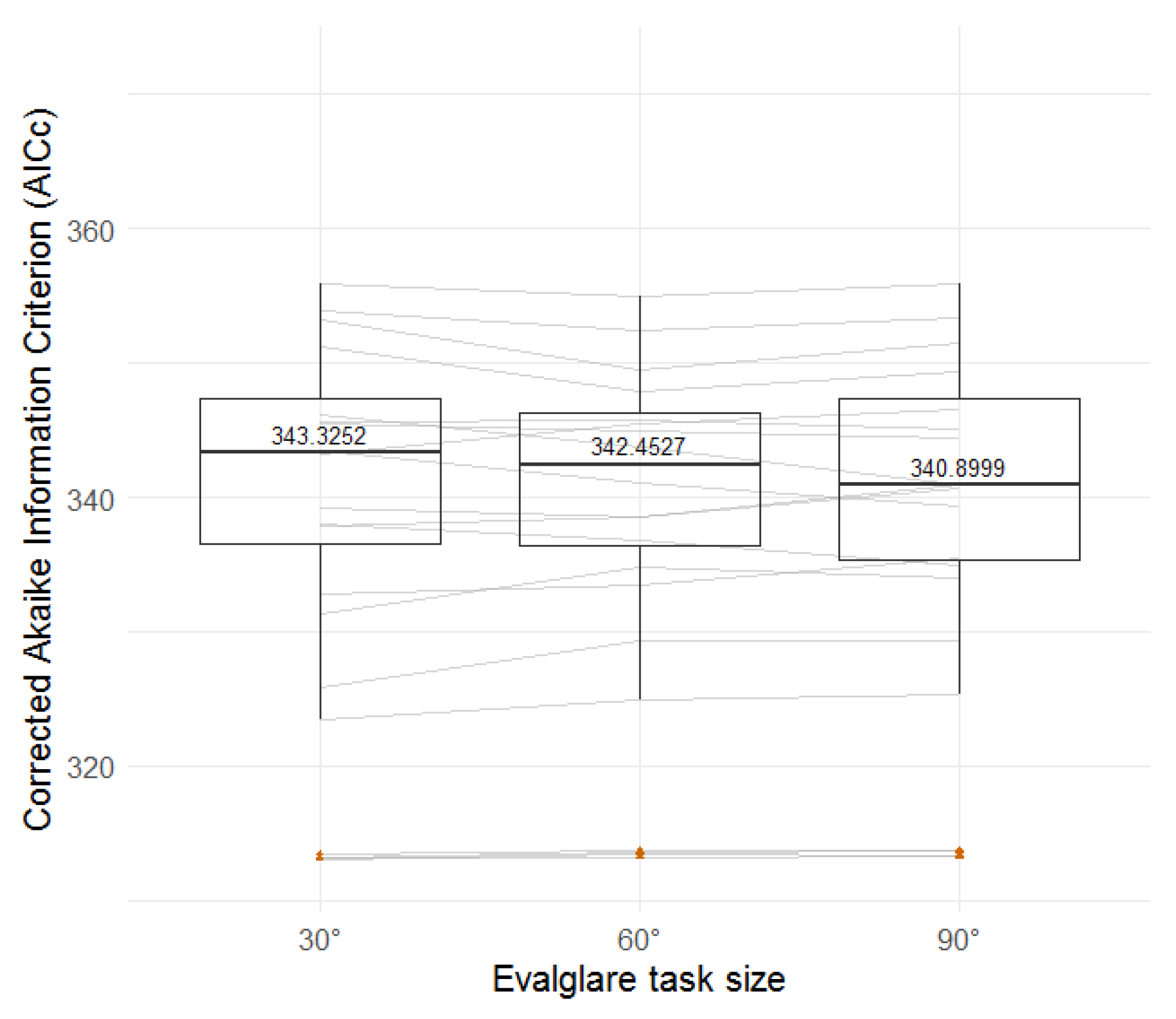
Figure 24, Figure 25, Figure 26, Figure 27, Figure 28 and Figure 29 show boxplots that are similar than the ones in Figure 12, Figure 13, Figure 14, Figure 15, Figure 16, Figure 17, Figure 18, Figure 19, Figure 20, Figure 21, Figure 22 and Figure 23, for both the field (left) and laboratory (right) studies, and for the three indicators of accuracy of discomfort glare prediction. However, in the case of the task area size parameter, each boxplot is based on a group of 16 datapoints. The 16 datapoints are the indicators corresponding to the four discomfort glare indices (DGI, CGI, DGImod, and UGP) and the four task area methods (t3, t4, t5, t6). The factor and threshold methods are left out of the boxplots since the variation due to the task area size has no influence on their accuracy of discomfort glare prediction. As the few non-significant statistics (Spearman correlation and logistic regressions) are found when using the factor method, all of the datapoints plotted in Figure 24, Figure 25, Figure 26, Figure 27, Figure 28 and Figure 29 are based on significant statistics. At last, the orange triangle points represent the indicators based on the DGP index.
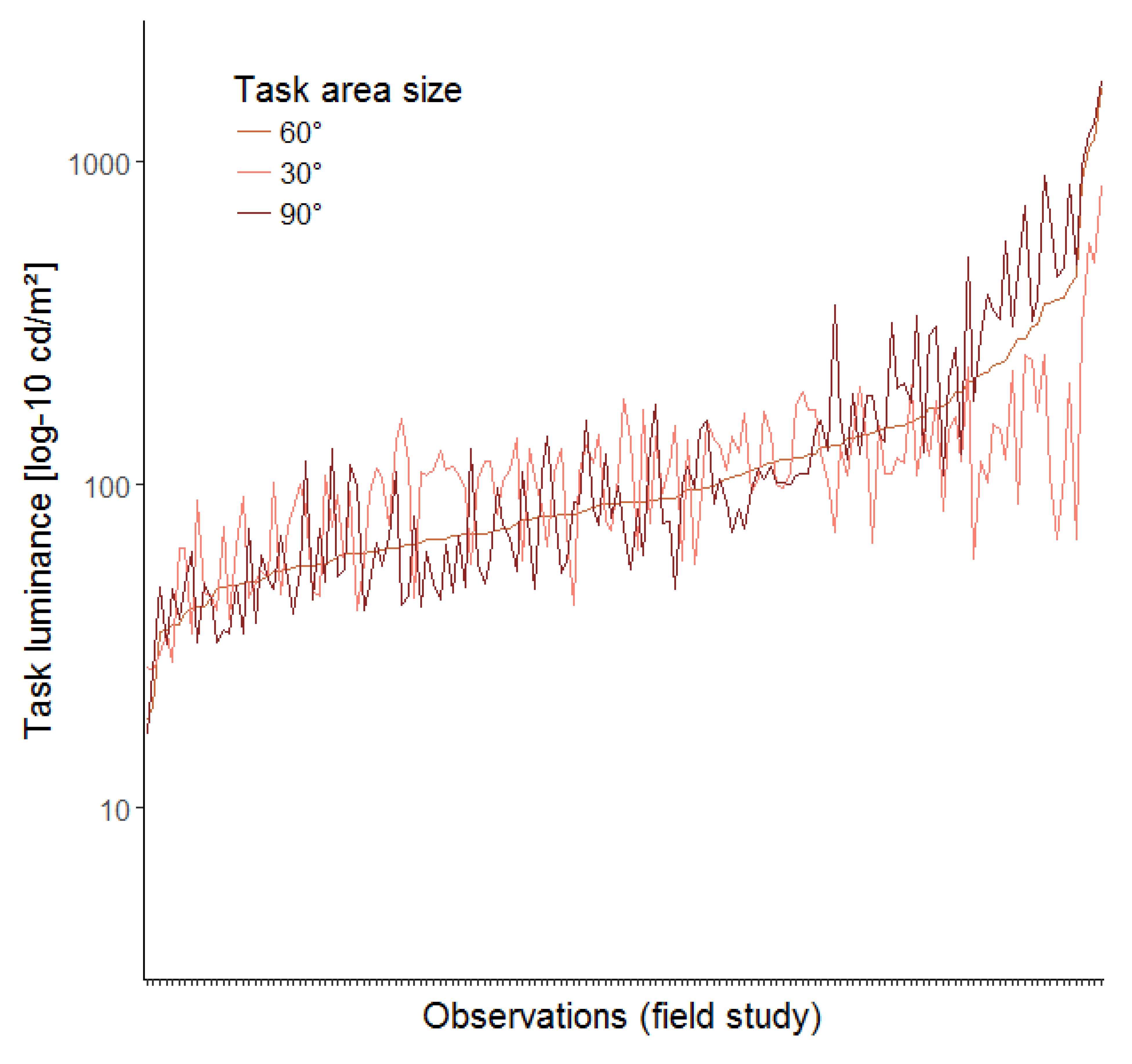
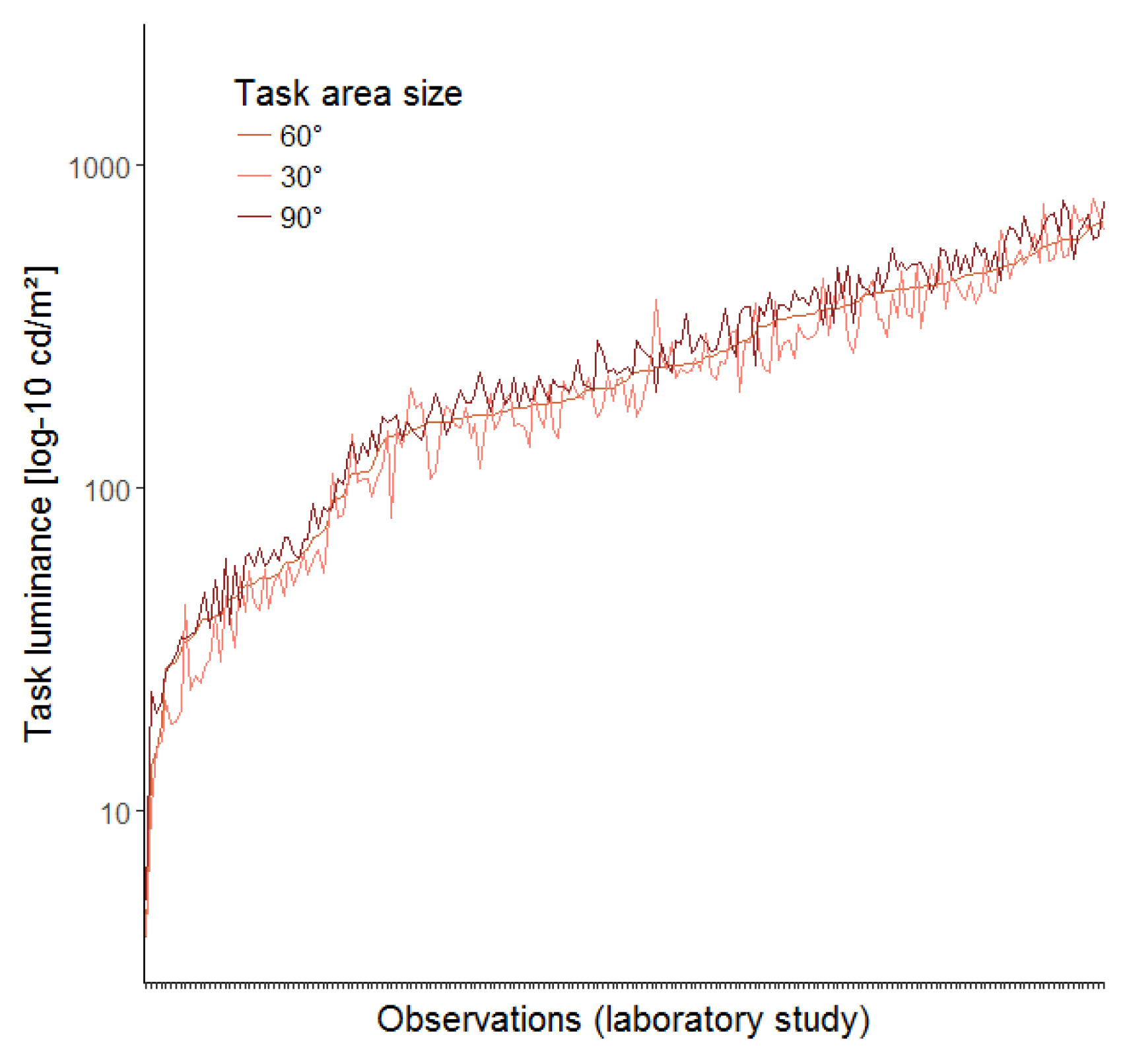
The overall accuracy of discomfort glare prediction can be compared on the boxplots between the three different task area sizes, having, respectively, an opening angle of 30° (0.52 rad.), 60° (1 rad.), and 90° (1.57 rad.). The 60° task area opening angle is what is believed to be commonly used in evalglare, as this corresponds to the ergorama. Varying the task area size might be interpreted as varying the size of the part of the field of view to which the subject’s eyes are adapting. But, increasing this task area size does not systematically mean increasing the average luminance of this task area; the visual scene will be determinant in this case. Figure 30 and Figure 31 help to understand the implication of varying the task area size on the average task luminance, and thus on the glare source detection threshold. For the laboratory study (Figure 31), the variation of the task area size has a small and relatively constant impact on the task luminance: the larger the task area size, the larger the task luminance. In the case of the field study (Figure 30), the impact of the variation of the task area size on the task luminance is larger, but more chaotic. This is due to the fact that, in real office settings, the field of view changes a lot from one desk to the other, hence the luminance distribution of this field of view varies a lot as well. In a laboratory setting, on the contrary, the visual field is relatively constant, causing the variation in the task luminance to be relatively constant as well.
However, it seems that a consistent variation of the glare source detection threshold—due to a consistent variation of the task luminance—does not produce a consistent influence on the accuracy of discomfort glare prediction. In the boxplots of the laboratory study (Figure 25, Figure 27 and Figure 29), the lines are crossing and going in opposite directions, which means that the influence of the task area size is not consistent throughout the discomfort glare indices or the task area methods. Moreover, the three indicators of the accuracy of discomfort glare prediction disagree on which would be the best task area size. At last, the significant difference scores between the three task area sizes for the laboratory study (Table 10) are low or equal to 0%. No conclusions can therefore be drawn from the analysis of the task area size influence while using the laboratory dataset.
On the other hand, from the boxplots of the field study (Figure 24, Figure 26 and Figure 28), a steady trend can be observed: by decreasing the task area size, the accuracy of discomfort glare prediction is increased. It is however quite difficult to explain this trend. What could be observed in Figure 30 is that when the task luminance is relatively low, using a smaller task area size tends to increase this task luminance; but when the task luminance is relatively high, using a smaller task area size tends to decrease the task luminance. A small task area size thus leads to a more constant task luminance throughout different visual scenes. A more accurate discomfort glare prediction could therefore be achieved thanks to the use of a less fluctuating eye adaptation level. In reality, it is indeed expected that the subject’s eyes adapt to the computer screen brightness, which should not vary a lot. However, the differences between the three task area sizes do not appear to be statistically significant, even for the field study (Table 11). More insight on the actual task area, namely the area of the field of view to which the subject’s eyes are really adapting, are required to better understand what can be seen here, and to determine an appropriate task area size.
4.5. Smooth Option
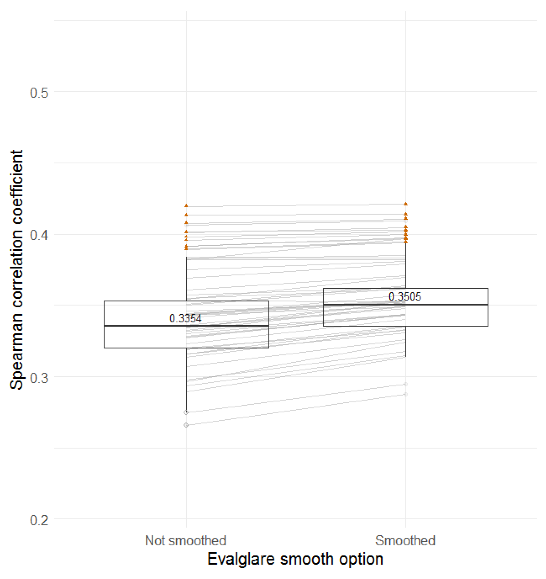
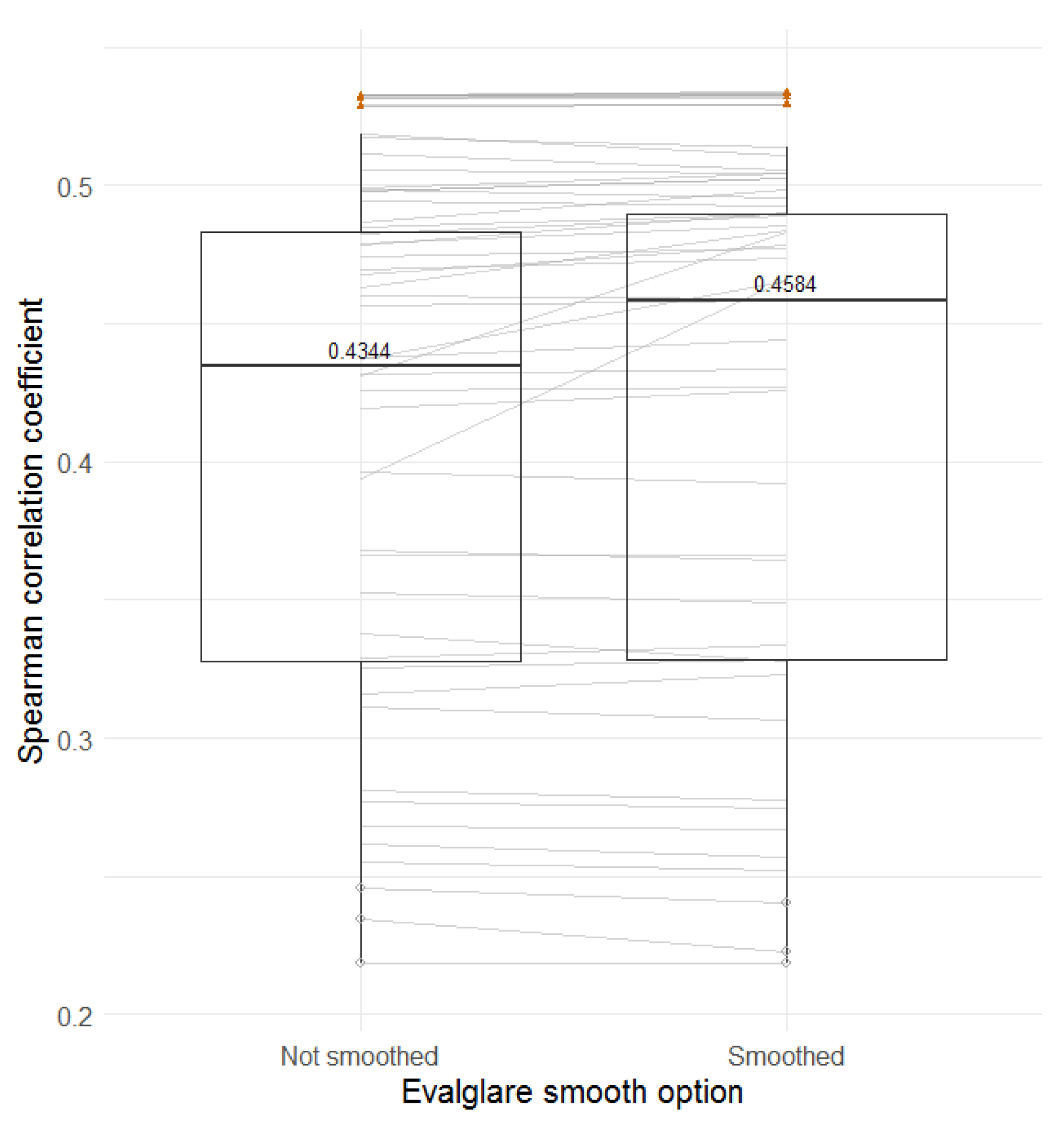
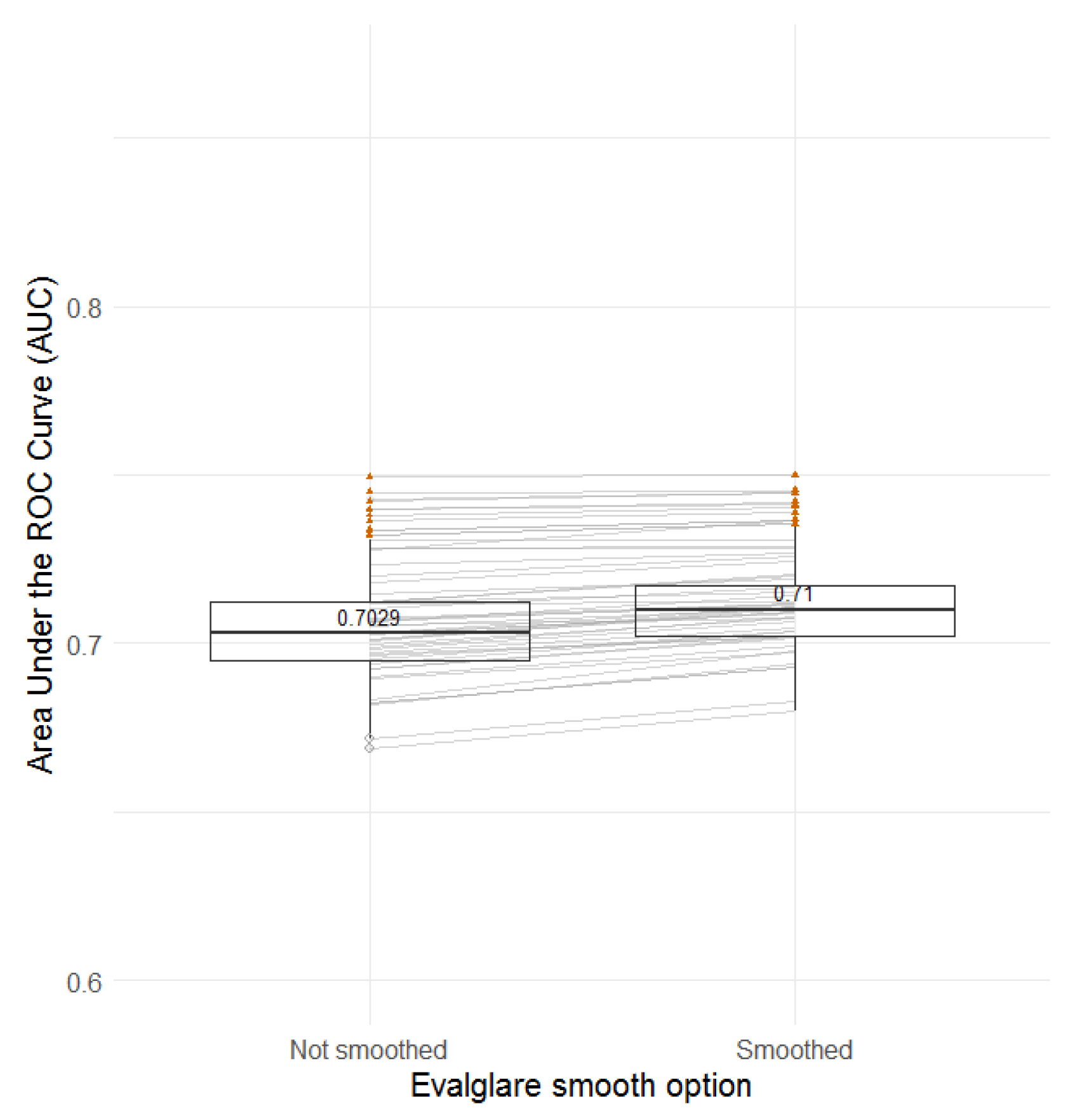
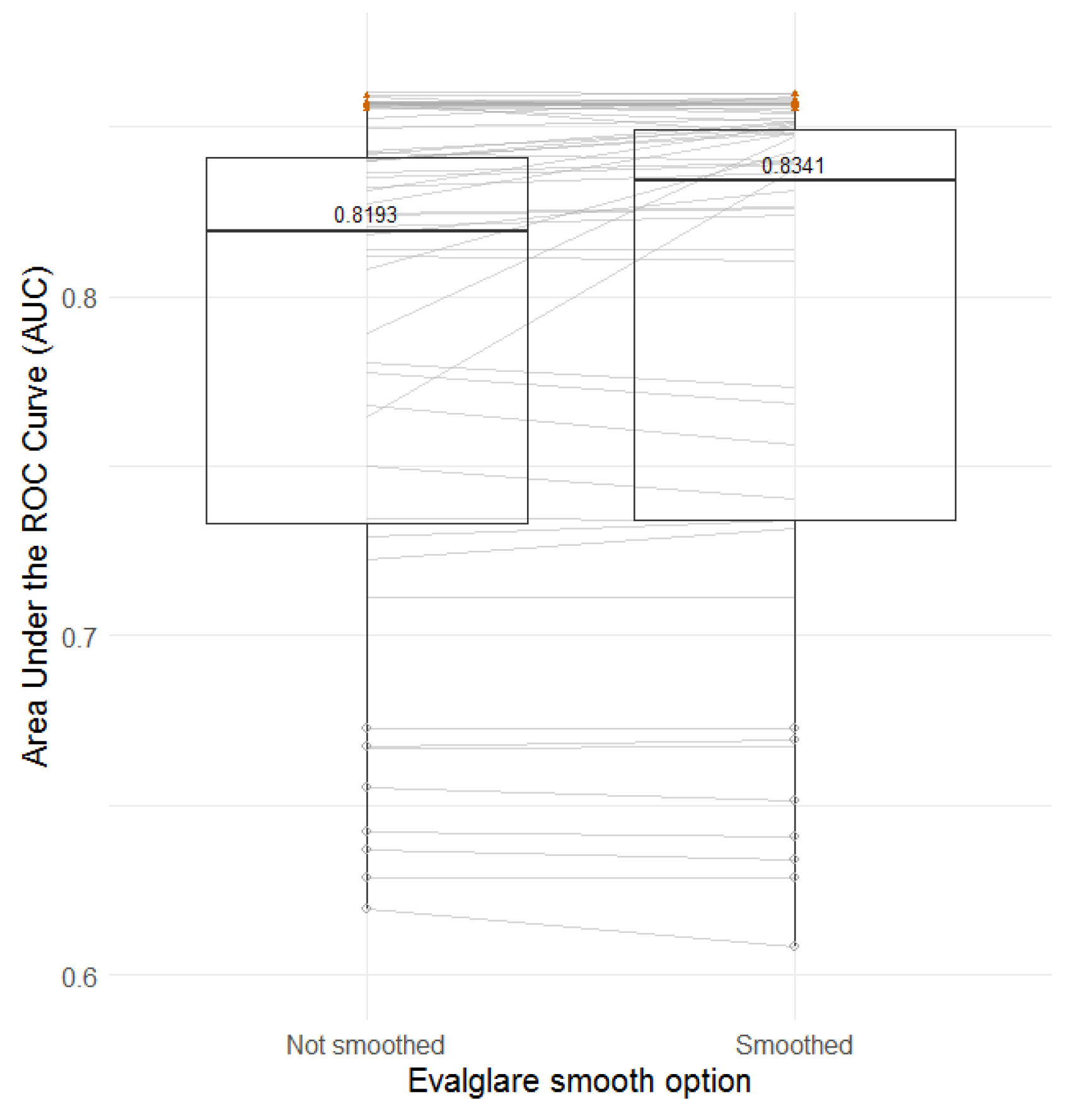
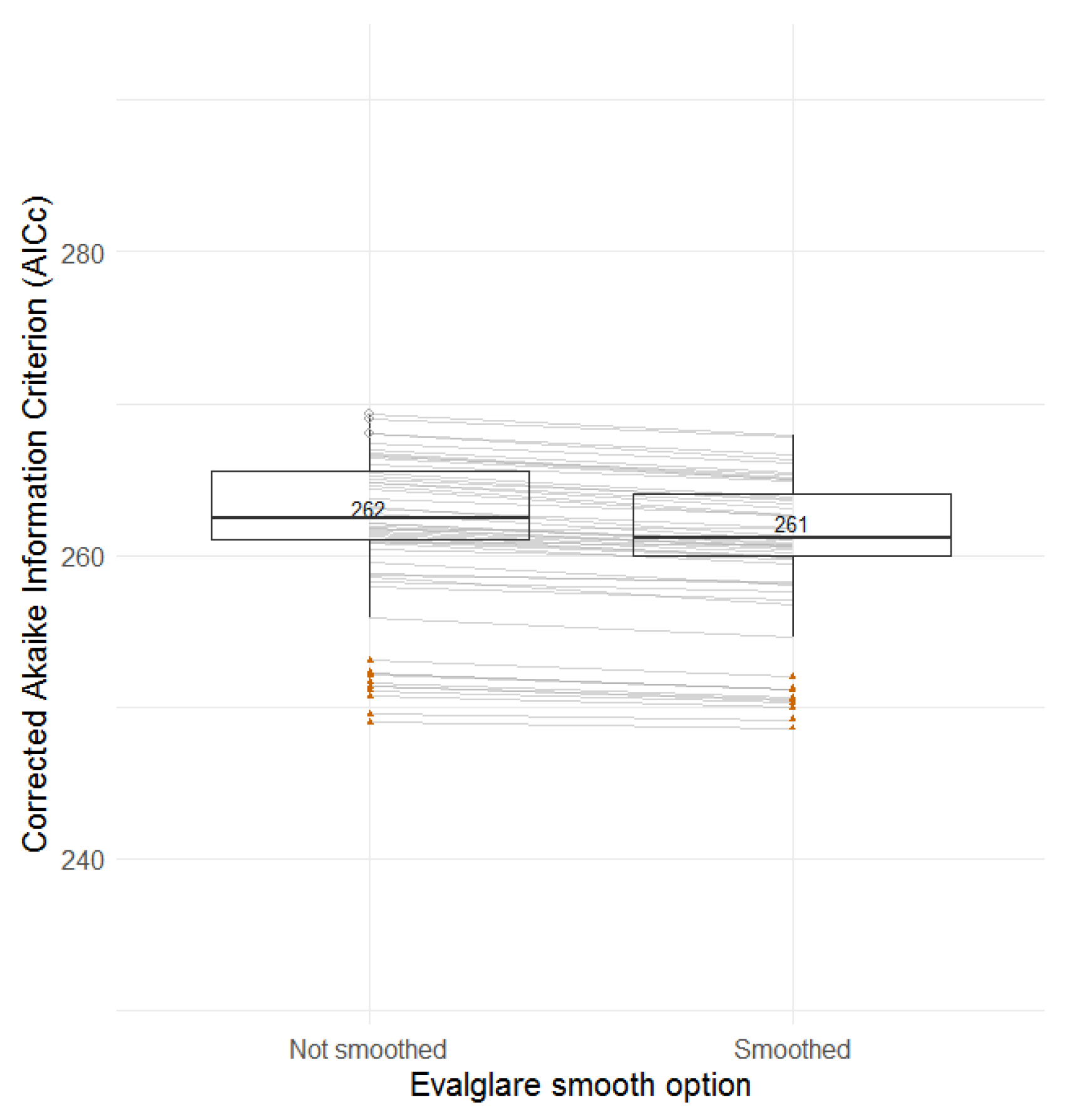
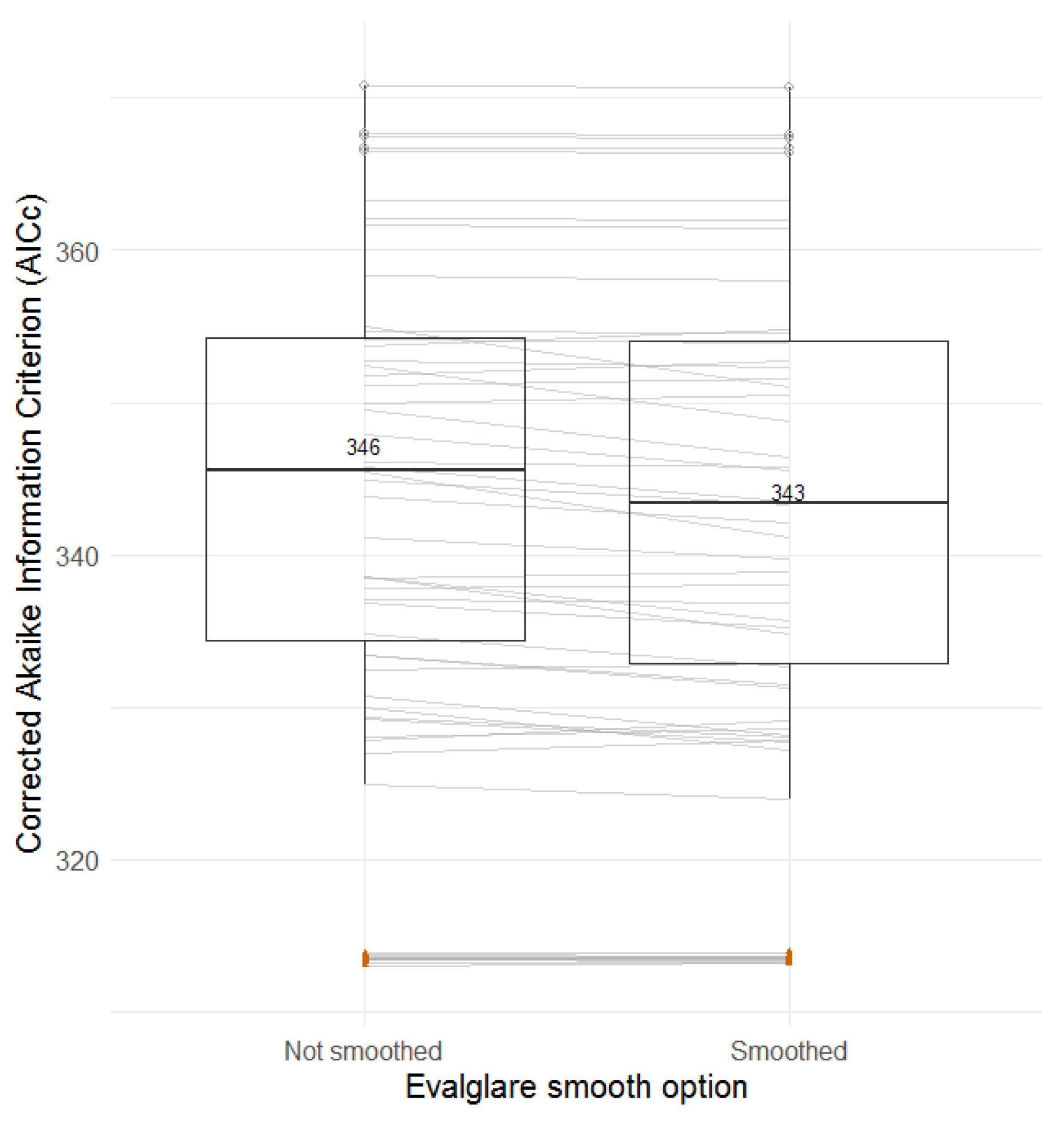
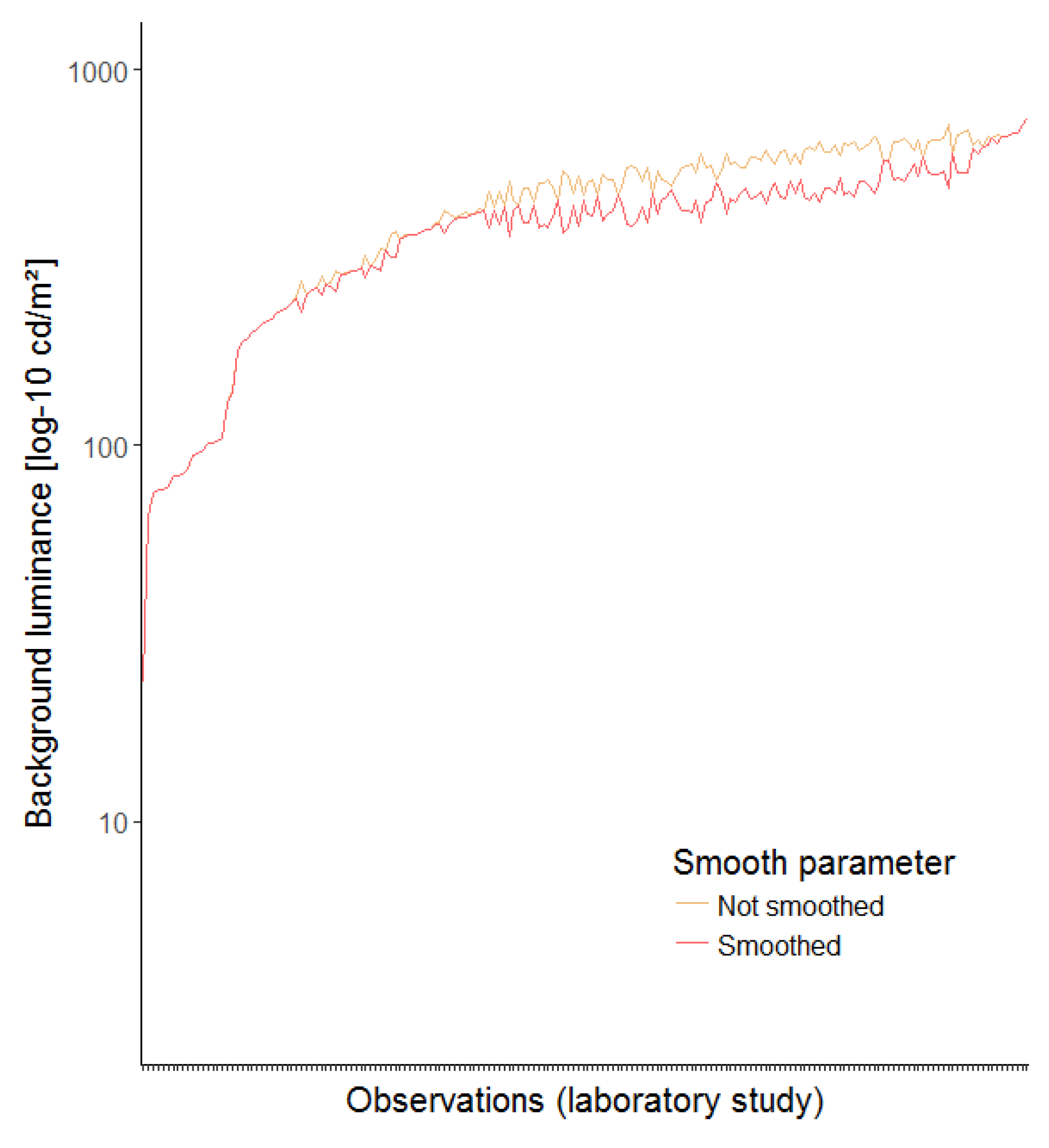
Figure 32, Figure 33, Figure 34, Figure 35, Figure 36 and Figure 37 compare the accuracy of discomfort glare prediction when the detected glare sources are smoothed or not. Using the smooth parameter causes the pixels that are not detected as glaring pixels by the algorithm, but that are nested inside an area of glaring pixels to be considered as glaring pixels as well and included in the surrounding glare source. Therefore, when the smooth parameter is applied, a detected glare source in a luminance map will have a larger solid angle, but a lower average luminance. The smooth parameter is presumably seldom used, mainly because it did not belong to the recommended options in evalglare, and little data have been published about it, making its contribution not well understood. In addition, its computation time is three to four times longer.
From the boxplots (Figure 32, Figure 33, Figure 34, Figure 35, Figure 36 and Figure 37), a general trend is observed towards a higher accuracy of discomfort glare prediction with the smooth parameter. This is especially visible for the field study, as the lines all go in the same direction. This implies that the influence of the smooth option is not dependent on the discomfort glare index that is used or the evalglare method applied. To understand why the smooth parameter offers a constant improvement of discomfort glare prediction, its impact on the four main physical quantities influencing discomfort glare [1] was investigated through the Glare Impact (GI). The GI was first introduced by [32], and it was redefined here, according to Equation (2).
with Ls,i, the luminance of the glare source;
ωi, the solid angle of the glare source;
Lb, the luminance of the background; and,
Pi, the position index related to the glare source.
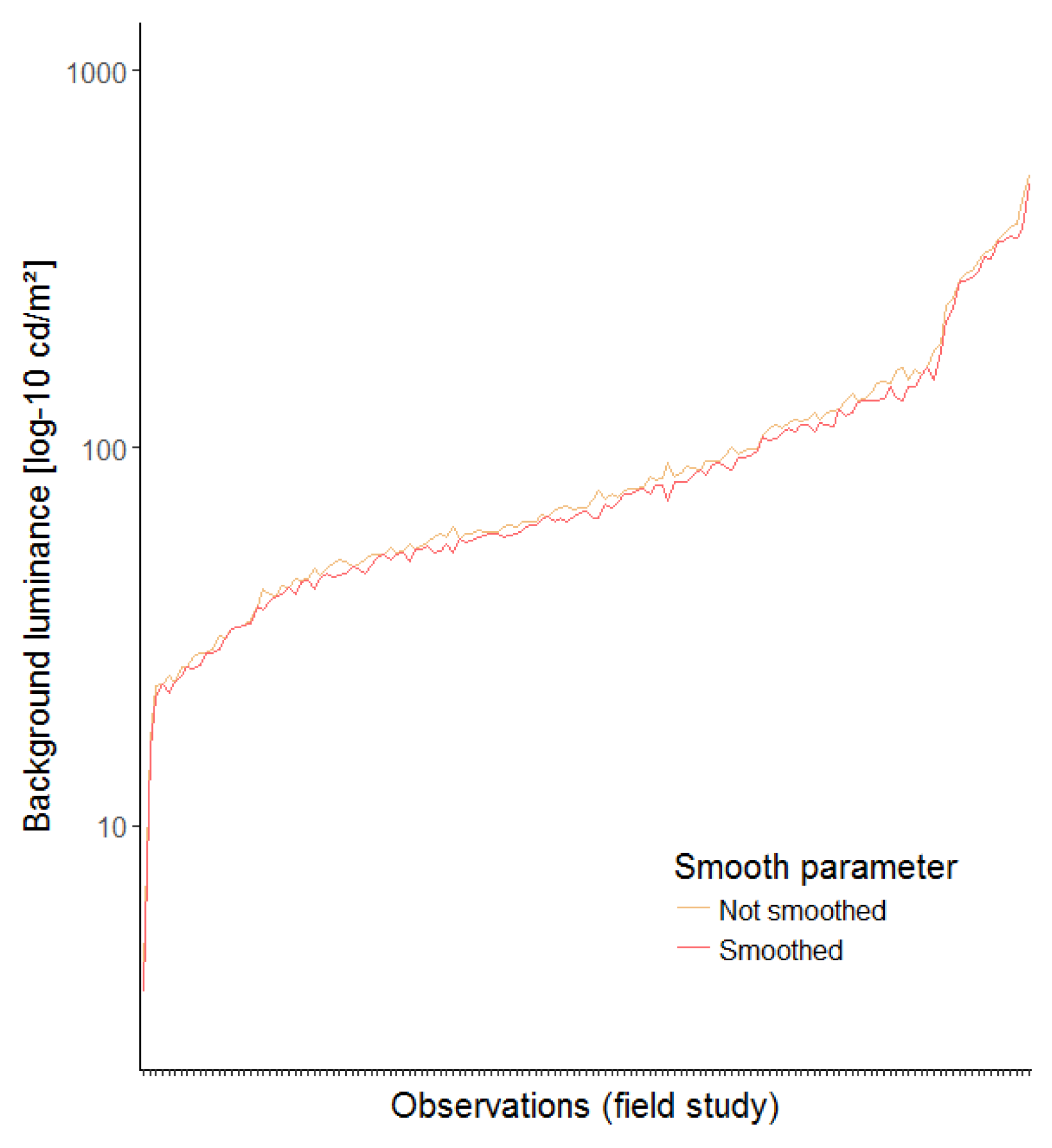
First, the variation of the GI according to the smooth parameter was studied. This did not help understanding the influence of the smooth parameter, since the variations of the GI due to the smoothing were not constant and very dependent on the visual scene. In bright visual scenes, a squared decrease in the average glare source luminance due to the use of the smooth parameter was generally balanced by the increase in the solid angle of this glare source. However, in low-light scenes, the squared decrease in the glare source luminance could most of the time not be entirely balanced by the increase in the solid angle. The only constant variation that is brought by the smooth parameter is the decrease in background luminance, as can be seen in Figure 38 and Figure 39. Since the originally non-glaring pixels located next to a glare source are included in this glare source due to the smoothing, the average background luminance is lowered as some of the brightest pixels of the background—those located next to a glare source—are retrieved from this background. The constant decrease in the background luminance due to the smoothing could thus be linked to the constant increase in the accuracy of discomfort glare perception.
Looking at the significant difference scores between the smooth/non-smooth parameter (Table 12 and Table 13), the differences in the accuracy of discomfort glare prediction can be considered to be statistically significant only for a few cases, especially in the field study. The smooth parameter appears not to produce a strong significant difference in the accuracy of discomfort glare prediction, despite a clear tendency towards a better glare prediction with the smooth parameter applied (Figure 32, Figure 33, Figure 34, Figure 35, Figure 36 and Figure 37).
The observations that are made here following the investigation of the smooth parameter should not lead to an excessive and indiscriminate use of this parameter, with the sole purpose to improve the correlation between the subjective glare ratings and the discomfort glare indices in a study. These results should first be validated in an extended study. Moreover, the settings choice in evalglare should always be done in an objective and sensible way, so as not to bias the results.
At last, the results that are presented here should be interpreted with respect to the limitations of the study. This study concentrated on the most common settings that are available in evalglare. However, other settings—such as the definition of the position index—might also influence the accuracy of discomfort glare prediction. Moreover, the observations are made based on a limited number of visual scenes. It is believed that the use of two different datasets brings a larger diversity in the studied visual scenes and their luminance distributions, making the results applicable to a large number of situations. But, different or extreme visual scenes could produce different results. Finally, these results are based on the five most common discomfort glare indices for daylighting. However, these indices are not performing as well as could be expected [33], and a lot of research is still going on to understand the mechanism behind discomfort glare perception and to determine an accurate way of measuring it. Moreover, one of these five indices, the DGP, possesses a validity range, which means that DGP values lower than 0.2 or higher than 0.8 should be interpreted with an additional layer of caution.
5. Conclusions
In this study, the influence of the choice of evalglare methods and parameters on the accuracy of discomfort glare prediction was investigated. The aim was to determine which method and parameters offer the best discomfort glare prediction for both types of discomfort glare, namely the contrast and saturation glare. Therefore, two datasets were used in this study, each one representative of one type of glare. In total, 63 different evalglare options were tested (Table 2), and for each option, five common daylight discomfort glare indices were calculated (DGP, DGI, CGI, DGImod, and UGP). Three statistical indicators were computed for each index, for each evalglare option, and for both datasets, so that the accuracy of discomfort glare prediction deriving from each evalglare option can be evaluated. These three statistical indicators are the Spearman correlation coefficient (or Spearman rho), the Area Under the ROC Curve of a binomial logistic regression model (or AUC), and the corrected Akaike’s Information Criterion of an ordinal logistic regression model (or AICc).
The results confirmed that the task area method should be preferred when evaluating visual scenes with contrast glare. For visual scenes where saturation glare is more predominant, the threshold method seems the most appropriate one, although the task area method offers very similar results. More specifically, the results showed that the task area method should be applied with a multiplying factor of 4 or 5, while the most appropriate threshold for the threshold method seems to be 2000 cd/m2, as is generally found in the literature. The calculation method of the background luminance—CIE definition or mathematical definition—seems to have no influence on the accuracy of discomfort prediction. A small trend could be observed for the influence of the search radius and the task area size parameter, although their influence on the accuracy of discomfort glare prediction could not be demonstrated as being statistically significant. The default search radius in evalglare, having an opening angle of 0.2 radians, was the one leading to the best discomfort glare prediction. As for the task area size, it seems that a smaller task area size, having an opening angle between 30° and 60°, would be more appropriate for discomfort glare prediction. However, more research involving datasets with different visual conditions is required to confirm these results. At last and quite surprisingly, applying the smooth parameter appeared to generate a more accurate discomfort glare prediction. It was hypothesized that this effect might be due to the decrease in background luminance when applying the smoothing. Rather than resulting in an unreasonable use of the smooth parameter to improve discomfort glare studies results, this observation should initiate the reconsideration of the basis of most discomfort glare indices nowadays, namely the Glare Impact formula (Equation (2)). Since it was observed that, for both studies, the accuracy of discomfort glare prediction was most certainly improved by decreasing the background luminance, the weighting or even the use of this physical quantity in discomfort glare models could be questioned. An extended laboratory study reassessing the influence of each one of the four main variables that is used in discomfort glare models (Ls, ω, Lb, and P) would be required, to validate the basis of the discomfort glare knowledge and to provide a clear definition of a glare source.
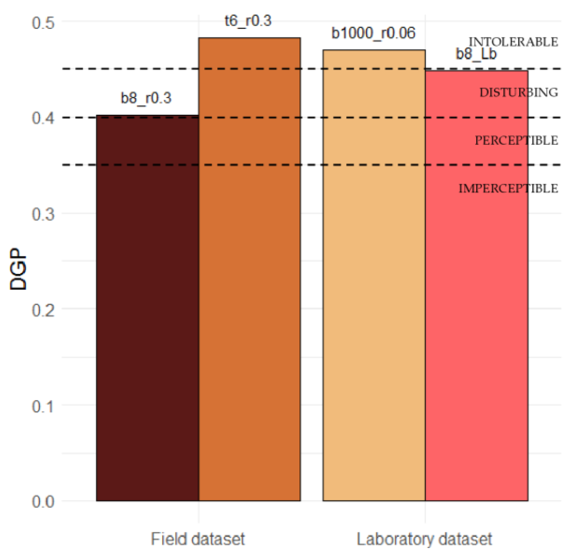
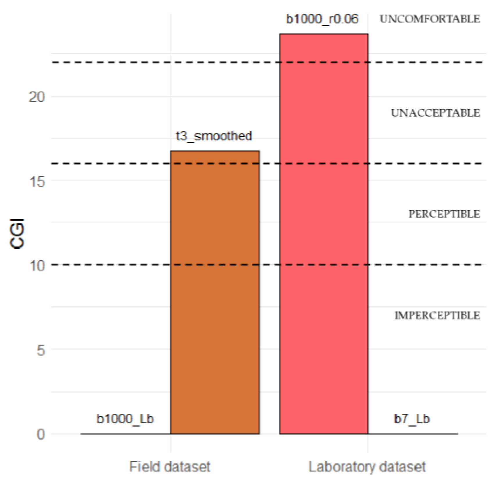
In addition, the authors would like to emphasize the importance of the choice of evalglare methods and parameters. When using evalglare, one should always be aware that this tool could lead to very different results in discomfort glare index calculation depending on these choices. Figure 40 and Figure 41 show extreme examples of such variations in discomfort glare indices values that were observed in the framework of this study. Although the DGP was found to be only slightly influenced by the detection parameters and methods in evalglare, the settings could matter as well for specific cases. In Figure 40, an extreme visual scene from each dataset would change from the “disturbing glare” category to the “intolerable glare” category (thresholds defined according to [34]) due to the use of different settings in evalglare. More extreme variations were observed for the four other discomfort glare indices (DGI, CGI, DGImod, and UGP) (Figure 41). In the given examples (Figure 42 and Figure 43), no glare source was found by using the b1000_Lb method for the field study example (Figure 42, left) or the b7_Lb method for the laboratory study example (Figure 43, right). The value of the CGI index corresponding to these two scenes is 0, and they are therefore categorized as “Imperceptible glare” (Figure 41). But, for other settings, such as the t3_smoothed method for the field study example (Figure 42, right) and the b1000_r0.06 method for the laboratory study example (Figure 43, left), glare sources are detected in the scenes. The same scenes are then categorized as “Unacceptable glare” or even “Uncomfortable glare” (thresholds defined according to [17,35]) (Figure 41). It is therefore strongly recommended to create a check file when using evalglare to calculate discomfort glare indices from a luminance map and examine visually the glare source(s) detected. The visual analysis of the glare sources is a useful way to verify that the glare sources detected are reasonable.
To conclude, for predominating saturation glare scenes, it would be beneficial to use an absolute threshold of 2000 cd/m2. This method should also be preferred for simulation work with an observer location close to the façade. Using the task area method with a factor 4 or 5 delivers for all of the investigated cases (saturation and contrast glare scenes) reasonable results and it is the preferred option for predominating contrast glare scenes. This method should be applied in simulation work, when the observer is located further away from the façade, although the task area definition might be sensitive. Using the factor method—evalglare default method—was found to lead to significantly lower performances and is therefore not recommended. From this study, the influences of the background luminance definition, the search radius, and the task area size were found to be not statistically significant. It is therefore recommended to use the default setting for these parameters. Further research on the definition of a glare source in daylighting is required, so that these parameters can be determined knowingly and reliably.
Author Contributions
Conceptualization, C.P., J.W. and M.B.; Methodology, C.P., J.W. and M.B.; Formal Analysis, C.P.; Investigation, C.P. and J.W.; Data Curation, C.P. and J.W.; Writing-Original Draft Preparation, C.P.; Writing-Review & Editing, J.M. and M.B.; Visualization, C.P.; Supervision, J.W. and M.B.; Project Administration, C.P.; Funding Acquisition, C.P. and M.B.
Funding
This research was funded by the Fonds de la Recherche Scientifique—FNRS.
Acknowledgments
The DE-Quanta study (laboratory study) was supported by the Fraunhofer-Institute for Solar Energy Systems ISE and the Deutsche Forschungsgemeinschaft DFG (WA1155/5-1).
Conflicts of Interest
The authors declare no conflict of interest. The founding sponsors had no role in the design of the study; in the collection, analyses, or interpretation of data; in the writing of the manuscript, and in the decision to publish the results.
References
- Commission Internationale de l’Eclairage (CIE). Discomfort Glare in the Interior Working Environment; Commission Internationale de l’Eclairage: Vienna, Austria, 1983; p. 52. [Google Scholar]
- Pierson, C.; Wienold, J.; Bodart, M. Review of factors influencing perceived discomfort glare from daylighting. J. Illum. Eng. Soc. N. Am. 2018, 14, 111–148. [Google Scholar]
- Wienold, J.; Christoffersen, J. Evaluation methods and development of a new glare prediction model for daylight environments with the use of ccd cameras. Energy Build. 2006, 38, 743–757. [Google Scholar] [CrossRef]
- Wienold, J.; Reetz, C.; Kuhn, T.E.; Christoffersen, J. Evalglare—A new radiance-based tool to evaluate daylight glare in office spaces. In Proceedings of the 3rd International Radiance Workshop, Fribourg, Switzerland, 11–12 October 2004. [Google Scholar]
- Wienold, J. New features of evalglare. In Proceedings of the 11th International Radiance Workshop, Copenhagen, Denmark, 12–14 September 2012. [Google Scholar]
- Wienold, J.; Andersen, M. Evalglare 2.0–new features faster and more robust hdr-image evaluation. In Proceedings of the 15th International Radiance Workshop, Padua, Italy, 29–31 August 2016. [Google Scholar]
- Wienold, J. Daylight Glare in Offices. Ph.D. Thesis, Universität Karlsruhe (TH), Freiburg, Germany, 2009. [Google Scholar]
- Jakubiec, J.A.; Reinhart, C.F. Diva 2.0: Integrating daylight and thermal simulations using rhinoceros 3d and energyplus. In Proceedings of the Building Simulation 2011 12th Conference of International Building Performance Simulation Association, Sydney, Australia, 14–16 November 2011. [Google Scholar]
- Pierson, C.; Piderit, M.B.; Wienold, J.; Bodart, M. Discomfort glare from daylighting: Influence of culture on discomfort glare perception. In Proceedings of the CIE 2017 Midterm Meeting, Jeju, Korea, 23–25 October 2017. [Google Scholar]
- Moosmann, C.; Wienold, J.; Wagner, A.; Wittwer, V. AbschluErmittlung Relevanter Einflussgrößen auf Die Subjektive Bewertung von Tageslicht zur Bewertung des Visuellen Komforts in Büroräumen. Abschlussbericht. 2012. Available online: https://publikationen.bibliothek.kit.edu/1000034968 (accessed on 6 June 2018).
- Dubois, M.-C. Impact of Shading Devices on Daylight Quality in Office—Simulations with Radiance; TABK–01/3062; Lund University: Lund, Sweden, 2001; p. 162. [Google Scholar]
- Shin, J.Y.; Yun, G.Y.; Kim, J.T. View types and luminance effects on discomfort glare assessment from windows. Energy Build. 2012, 46, 139–145. [Google Scholar] [CrossRef]
- Bülow-Hübe, H. Daylight in Glazed Office Buildings—A Comparative Study of Daylight Availability, Luminance and Illuminance Distribution for an Office Room with Three Different Glass Areas; EBD-R--08/17; Lund University: Lund, Sweden, 2008; p. 98. [Google Scholar]
- Lee, E.S.; Clear, R.D.; Fernandes, L.; Ward, G. Commissioning and Verification Procedures for the Automated Roller Shade System at the New York Times Headquarters, New York; Lawrence Berkeley National Laboratory (LBNL): Berkeley, CA, USA, 2007; p. 112.
- Van Den Wymelenberg, K.; Inanici, M.; Johnson, P. The effect of luminance distribution patterns on occupant preference in a daylit office environment. J. Illum. Eng. Soc. 2010, 7, 103–122. [Google Scholar]
- Chauvel, P.; Collins, J.B.; Dogniaux, R.; Longmore, J. Glare from windows: Current views of the problem. Light. Res. Technol. 1982, 14, 31–46. [Google Scholar] [CrossRef]
- Einhorn, H.D. Discomfort glare: A formula to bridge differences. Light. Res. Technol. 1979, 11, 90–94. [Google Scholar] [CrossRef]
- Fisekis, K.; Davies, M.; Kolokotroni, M.; Langford, P. Prediction of discomfort glare from windows. Light. Res. Technol. 2003, 35, 360–371. [Google Scholar] [CrossRef]
- Hirning, M.B.; Isoardi, G.L.; Cowling, I. Discomfort glare in open plan green buildings. Energy Build. 2014, 70, 427–440. [Google Scholar] [CrossRef] [Green Version]
- Siegel, S. Nonparametric Statistics for the Behavioral Sciences; McGraw-Hill Book Company: New York, NY, USA, 1956. [Google Scholar]
- Ferguson, C.J. An effect size primer: A guide for clinicians and researchers. Prof. Psychol. Res. Pract. 2009, 40, 532–538. [Google Scholar] [CrossRef]
- Diedenhofen, B.; Musch, J. Cocor: A comprehensive solution for the statistical comparison of correlations. PLoS ONE 2015, 10, e0121945. [Google Scholar] [CrossRef] [PubMed]
- Hosmer, D.W.; Lemeshow, S. Applied Logistic Regression, 2nd ed; Wiley: Toronto, ON, Canada, 2000. [Google Scholar]
- Safari, S.; Baratloo, A.; Elfil, M.; Negida, A. Evidence based emergency medicine; part 5 receiver operating curve and area under the curve. Emergency 2016, 4, 111–113. [Google Scholar] [PubMed]
- Venkatraman, E.S.; Begg, C.B. A distribution-free procedure for comparing receiver operating characteristic curves from a paired experiment. Biometrika 1996, 83, 835–848. [Google Scholar] [CrossRef]
- DeLong, E.R.; DeLong, D.M.; Clarke-Pearson, D.L. Comparing the areas under two or more correlated receiver operating characteristic curves: A nonparametric approach. Biometrics 1988, 44, 837–845. [Google Scholar] [CrossRef] [PubMed]
- Pepe, M.; Longton, G.; Janes, H. Estimation and Comparison of Receiver Operating Characteristic Curves; Biostatistics Working Paper Series; The Berkeley Electronic Press: Berkeley, CA, USA, 2008. [Google Scholar]
- Murtaugh, P.A. In defense of p values. Ecology 2014, 95, 611–617. [Google Scholar] [CrossRef] [PubMed]
- Burnham, K.P.; Anderson, D.R. Model Selection and Multimodel Inference: A Practical Information-Theoretic Approach, 2nd ed.; Springer-Verlag: New York, NY, USA, 2002. [Google Scholar]
- Brewer, M.J.; Butler, A. Model Selection and the Cult of Aic; Universitat Autònoma de Barcelona: Barcelona, Spain, 2017. [Google Scholar]
- Hurvich, C.M.; Tsai, C.-L. Regression and time series model selection in small samples. Biometrika 1989, 76, 297–307. [Google Scholar] [CrossRef]
- Sarey Khanie, M.; Jia, Y.; Wienold, J.; Andersen, M. A sensitivity analysis on glare detection parameters. In Proceedings of the BS2015-14th International Conference of the International Building Performance Simulation Association, Hyderabad, India, 7–9 December 2015. [Google Scholar]
- Suk, J.Y.; Schiler, M.; Kensek, K. Investigation of existing discomfort glare indices using human subject study data. Build. Environ. 2017, 113, 121–130. [Google Scholar] [CrossRef]
- Reinhart, C.; Wienold, J. The daylighting dashboard—A simulation-based design analysis for daylit spaces. Build. Environ. 2011, 46, 386–396. [Google Scholar] [CrossRef]
- Boyce, P.R. Human Factors in Lighting, 3rd ed.; Taylor & Francis Group: Boca Raton, FL, USA, 2014; p. 690. [Google Scholar]
Figure 1.
Boxplots of vertical illuminance at eye level between the field study and the laboratory study.
Figure 1.
Boxplots of vertical illuminance at eye level between the field study and the laboratory study.

Figure 2.
Binary transformation (no discomfort–discomfort) of the subjective glare scales used in the field and laboratory studies.
Figure 2.
Binary transformation (no discomfort–discomfort) of the subjective glare scales used in the field and laboratory studies.

Figure 3.
Graph of the Receiver Operating Characteristic (ROC) curve corresponding to the binary logistic regression model computed for the Daylight Glare Probability (DGP) index calculated with t4_def evalglare option on the field study dataset (AUC = 0.7496).
Figure 3.
Graph of the Receiver Operating Characteristic (ROC) curve corresponding to the binary logistic regression model computed for the Daylight Glare Probability (DGP) index calculated with t4_def evalglare option on the field study dataset (AUC = 0.7496).

Figure 4.
Comparison of Spearman rho for each discomfort glare index between the studied evalglare methods (field study).
Figure 4.
Comparison of Spearman rho for each discomfort glare index between the studied evalglare methods (field study).

Figure 5.
Comparison of Spearman rho for each discomfort glare index between the studied evalglare methods (laboratory study).
Figure 5.
Comparison of Spearman rho for each discomfort glare index between the studied evalglare methods (laboratory study).

Figure 6.
Comparison of Area Under the Curve (AUC) for each discomfort glare index between the studied evalglare methods (field study).
Figure 6.
Comparison of Area Under the Curve (AUC) for each discomfort glare index between the studied evalglare methods (field study).

Figure 7.
Comparison of AUC for each discomfort glare index between the studied evalglare methods (laboratory study).
Figure 7.
Comparison of AUC for each discomfort glare index between the studied evalglare methods (laboratory study).

Figure 8.
Comparison of Akaike’s Information Criterion (AICc) for each discomfort glare index between the studied evalglare methods (field study).
Figure 8.
Comparison of Akaike’s Information Criterion (AICc) for each discomfort glare index between the studied evalglare methods (field study).

Figure 9.
Comparison of AICc for each discomfort glare index between the studied evalglare methods (laboratory study).
Figure 9.
Comparison of AICc for each discomfort glare index between the studied evalglare methods (laboratory study).

Figure 10.
Glare source detection by evalglare factor 5 method for a visual scene of the field study.
Figure 10.
Glare source detection by evalglare factor 5 method for a visual scene of the field study.

Figure 11.
Glare source detection by evalglare factor 7 method for a visual scene of the laboratory study.
Figure 11.
Glare source detection by evalglare factor 7 method for a visual scene of the laboratory study.

Figure 12.
Boxplots of Spearman rho for the two background luminance definitions (field study).

Figure 13.
Boxplots of Spearman rho for the two background luminance definitions (laboratory study).
Figure 13.
Boxplots of Spearman rho for the two background luminance definitions (laboratory study).

Figure 14.
Boxplots of AUC for the two background luminance definitions (field study).

Figure 15.
Boxplots of AUC for the two background luminance definitions (laboratory study).

Figure 16.
Boxplots of AICc for the two background luminance definitions (field study).

Figure 17.
Boxplots of AICc for the two background luminance definitions (laboratory study).

Figure 18.
Boxplots of Spearman rho for the three search radius (field study).

Figure 19.
Boxplots of Spearman rho for the three search radius (laboratory study).

Figure 20.
Boxplots of AUC for the three search radius (field study).

Figure 21.
Boxplots of AUC for the three search radius (laboratory study).

Figure 22.
Boxplots of AICc for the three search radius (field study).

Figure 23.
Boxplots of AICc for the three search radius (laboratory study).

Figure 24.
Boxplots of Spearman rho for the three task area sizes (field study).

Figure 25.
Boxplots of Spearman rho for the three task area sizes (laboratory study).

Figure 26.
Boxplots of AUC for the three task area sizes (field study).

Figure 27.
Boxplots of AUC for the three task area sizes (laboratory study).

Figure 28.
Boxplots of AICc for the three task area sizes (field study).

Figure 29.
Boxplots of AICc for the three task area sizes (laboratory study).

Figure 30.
Comparison of the task area average luminance between the three different task area sizes for all glare evaluations of the field study.
Figure 30.
Comparison of the task area average luminance between the three different task area sizes for all glare evaluations of the field study.

Figure 31.
Comparison of the task area average luminance between the 3 different task area sizes for all glare evaluations of the lab study.
Figure 31.
Comparison of the task area average luminance between the 3 different task area sizes for all glare evaluations of the lab study.

Figure 32.
Boxplots of Spearman rho for the non-smooth/smooth parameter (field study).

Figure 33.
Boxplots of Spearman rho for the non-smooth/smooth parameter (laboratory study).

Figure 34.
Boxplots of AUC for the non-smooth/smooth parameter (field study).

Figure 35.
Boxplots of AUC for the non-smooth/smooth parameter (laboratory study).

Figure 36.
Boxplots of AICc for the non-smooth/smooth parameter (field study).

Figure 37.
Boxplots of AICc for the non-smooth/smooth parameter (laboratory study).

Figure 38.
Comparison of the background luminance while varying the smooth parameter with the t4 method (task area method with a factor 4), for all glare evaluations of the field study.
Figure 38.
Comparison of the background luminance while varying the smooth parameter with the t4 method (task area method with a factor 4), for all glare evaluations of the field study.

Figure 39.
Comparison of the background luminance while varying the smooth parameter with the b2000 method (method with a threshold of 2000 cd/m2), for all glare evaluations of the laboratory study.
Figure 39.
Comparison of the background luminance while varying the smooth parameter with the b2000 method (method with a threshold of 2000 cd/m2), for all glare evaluations of the laboratory study.

Figure 40.
DGP of the same visual scene for different evalglare methods and parameters (field and laboratory studies).
Figure 40.
DGP of the same visual scene for different evalglare methods and parameters (field and laboratory studies).

Figure 41.
Commission on Illumination Glare Index (CGI) of the same visual scene for different evalglare methods and parameters (field and laboratory studies).
Figure 41.
Commission on Illumination Glare Index (CGI) of the same visual scene for different evalglare methods and parameters (field and laboratory studies).

Figure 42.
Extreme example (field study) of the difference in glare source(s) detection resulting from the b1000_Lb setting (left) and the t3_smoothed setting (right) in evalglare.
Figure 42.
Extreme example (field study) of the difference in glare source(s) detection resulting from the b1000_Lb setting (left) and the t3_smoothed setting (right) in evalglare.

Figure 43.
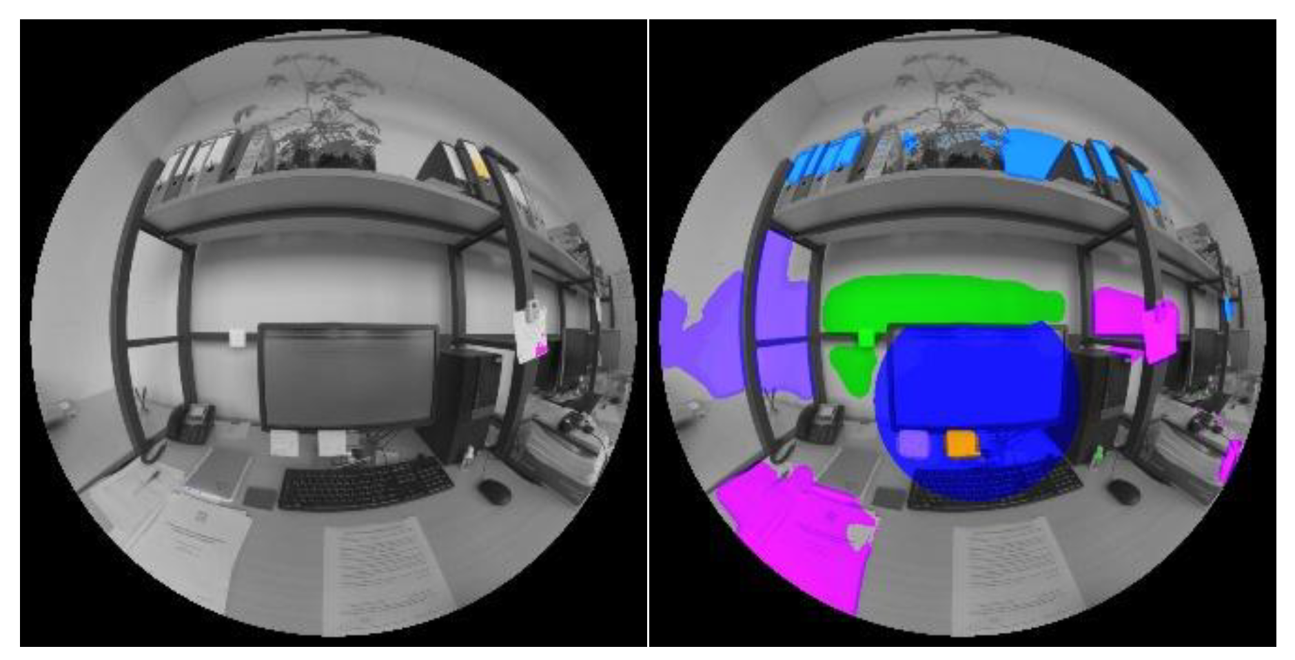
Extreme example (laboratory study) of the difference in glare source(s) detection resulting from the b1000_r0.06 setting (left) and the b7_Lb setting (right) in evalglare.
Figure 43.
Extreme example (laboratory study) of the difference in glare source(s) detection resulting from the b1000_r0.06 setting (left) and the b7_Lb setting (right) in evalglare.


Table 1.
Demographic and general information of field and laboratory datasets.
| Experiment | Subjects | Men/Women Ratio (%) | Mean Age (SD) | Glare Evaluations | 4-Point Glare Scale | Glare Rating Ratio (%) |
|---|---|---|---|---|---|---|
| Field study | 82 | 43/57 | 36 (11) | 141 | No discomfort A small discomfort A moderate discomfort A large discomfort | 65 20 11 4 |
| Laboratory study | 41 | 73/27 | 26 (3) | 180 | Imperceptible Noticeable Disturbing Intolerable | 53 30 17 1 |
Table 2.
Example of a visual scene from the lab study of differences in glare source detection for all of the evalglare options tested.
Table 2.
Example of a visual scene from the lab study of differences in glare source detection for all of the evalglare options tested.
| def | r0.06 | r0.3 | Lb | sm | ta0.52 | ta1.57 | |
| b5 |   | ||||||
| b6 | |||||||
| b7 | |||||||
| b8 | |||||||
| b1000 | |||||||
| b2000 | |||||||
| b4000 | |||||||
| t3 | |||||||
| t4 | |||||||
| t5 | |||||||
| t6 | |||||||
Table 3.
Grand mean of each discomfort glare index value for both datasets.
| Experiment | DGP | DGI | CGI | DGImod | UGP |
|---|---|---|---|---|---|
| Field study | 0.19 | 11.55 | 12.18 | 17.76 | 0.49 |
| Laboratory study | 0.33 | 11.82 | 12.6 | 18.85 | 0.5 |
Table 4.
Significant difference scores (%) between each tested method (field study).
| b5 | b6 | b7 | b8 | b1000 | b2000 | b4000 | t3 | t4 | t5 | |
|---|---|---|---|---|---|---|---|---|---|---|
| t6 | 2 | 0 | 10 | 36 | 0 | 0 | 0 | 0 | 15 | 6 |
| t5 | 11 | 0 | 16 | 40 | 13 | 0 | 0 | 2 | 2 | |
| t4 | 24 | 28 | 40 | 79 | 19 | 13 | 7 | 0 | ||
| t3 | 0 | 0 | 0 | 27 | 0 | 0 | 0 | |||
| b4000 | 0 | 0 | 0 | 0 | 0 | 2 | ||||
| b2000 | 0 | 2 | 22 | 33 | 0 | |||||
| b1000 | 0 | 0 | 7 | 27 | ||||||
| b8 | 26 | 43 | 44 | |||||||
| b7 | 2 | 6 | ||||||||
| b6 | 2 |
Table 5.
Significant difference scores (%) between each tested method (laboratory study).
| b5 | b6 | b7 | b8 | b1000 | b2000 | b4000 | t3 | t4 | t5 | |
|---|---|---|---|---|---|---|---|---|---|---|
| t6 | 20 | 33 | 71 | 80 | 16 | 42 | 20 | 20 | 11 | 27 |
| t5 | 38 | 60 | 80 | 80 | 13 | 20 | 13 | 0 | 0 | |
| t4 | 27 | 67 | 80 | 80 | 7 | 20 | 13 | 7 | ||
| t3 | 33 | 60 | 67 | 80 | 7 | 29 | 13 | |||
| b4000 | 82 | 80 | 80 | 80 | 7 | 0 | ||||
| b2000 | 80 | 80 | 80 | 80 | 20 | |||||
| b1000 | 38 | 62 | 80 | 80 | ||||||
| b8 | 80 | 73 | 7 | |||||||
| b7 | 73 | 22 | ||||||||
| b6 | 24 |
Table 6.
Significant difference scores (%) between the two background luminance definitions (field study).
Table 6.
Significant difference scores (%) between the two background luminance definitions (field study).
| b5 | b6 | b7 | b8 | b1000 | b2000 | b4000 | t3 | t4 | t5 | t6 | |
|---|---|---|---|---|---|---|---|---|---|---|---|
| CIE Lb >< Math. Lb | 0 | 0 | 6 | 6 | 0 | 0 | 2 | 2 | 0 | 0 | 0 |
Table 7.
Significant difference scores (%) between the two background luminance definitions (lab. study).
Table 7.
Significant difference scores (%) between the two background luminance definitions (lab. study).
| b5 | b6 | b7 | b8 | b1000 | b2000 | b4000 | t3 | t4 | t5 | t6 | |
|---|---|---|---|---|---|---|---|---|---|---|---|
| CIE Lb >< Math. Lb | 0 | 0 | 0 | 9 | 13 | 12 | 0 | 0 | 0 | 0 | 0 |
Table 8.
Significant difference scores (%) between the three search radius (field study).
| b5 | b6 | b7 | b8 | b1000 | b2000 | b4000 | t3 | t4 | t5 | t6 | |
|---|---|---|---|---|---|---|---|---|---|---|---|
| r0.2 >< r0.06 | 0 | 12 | 7 | 0 | 0 | 2 | 10 | 2 | 2 | 2 | 2 |
| r0.2 >< r0.3 | 2 | 0 | 0 | 0 | 0 | 0 | 0 | 62 | 22 | 0 | 0 |
| r0.06 >< r0.3 | 0 | 13 | 7 | 11 | 0 | 0 | 13 | 20 | 0 | 0 | 0 |
Table 9.
Significant difference scores (%) between the three search radius (laboratory study).
| b5 | b6 | b7 | b8 | b1000 | b2000 | b4000 | t3 | t4 | t5 | t6 | |
|---|---|---|---|---|---|---|---|---|---|---|---|
| r0.2 >< r0.06 | 13 | 0 | 4 | 0 | 6 | 4 | 0 | 15 | 27 | 40 | 40 |
| r0.2 >< r0.3 | 0 | 0 | 6 | 0 | 0 | 0 | 0 | 18 | 24 | 0 | 0 |
| r0.06 >< r0.3 | 15 | 0 | 2 | 0 | 6 | 0 | 0 | 16 | 9 | 33 | 40 |
Table 10.
Significant difference scores (%) between the three task area sizes (laboratory study).
| t3 | t4 | t5 | t6 | |
|---|---|---|---|---|
| 60° X 30° | 0 | 6 | 6 | 0 |
| 60° X 90° | 2 | 0 | 24 | 13 |
| 30° X 90° | 0 | 0 | 0 | 0 |
Table 11.
Significant difference scores (%) between the three task area sizes (field study).
| t3 | t4 | t5 | t6 | |
|---|---|---|---|---|
| 60° X 30° | 0 | 0 | 0 | 0 |
| 60° X 90° | 0 | 16 | 0 | 26 |
| 30° X 90° | 0 | 0 | 2 | 10 |
Table 12.
Significant difference scores (%) between the smooth/non-smooth parameter (field study).
| b5 | b6 | b7 | b8 | b1000 | b2000 | b4000 | t3 | t4 | t5 | t6 | |
|---|---|---|---|---|---|---|---|---|---|---|---|
| Smooth >< Non-smooth | 12 | 24 | 44 | 49 | 2 | 16 | 31 | 0 | 0 | 27 | 29 |
Table 13.
Significant difference scores (%) between the smooth/non-smooth parameter (laboratory study).
Table 13.
Significant difference scores (%) between the smooth/non-smooth parameter (laboratory study).
| b5 | b6 | b7 | b8 | b1000 | b2000 | b4000 | t3 | t4 | t5 | t6 | |
|---|---|---|---|---|---|---|---|---|---|---|---|
| Smooth >< Non-smooth | 0 | 0 | 0 | 0 | 0 | 0 | 19 | 0 | 0 | 7 | 35 |
© 2018 by the authors. Licensee MDPI, Basel, Switzerland. This article is an open access article distributed under the terms and conditions of the Creative Commons Attribution (CC BY) license (http://creativecommons.org/licenses/by/4.0/).
Share and Cite
MDPI and ACS Style
Pierson, C.; Wienold, J.; Bodart, M. Daylight Discomfort Glare Evaluation with Evalglare: Influence of Parameters and Methods on the Accuracy of Discomfort Glare Prediction. Buildings 2018, 8, 94. https://doi.org/10.3390/buildings8080094
AMA Style
Pierson C, Wienold J, Bodart M. Daylight Discomfort Glare Evaluation with Evalglare: Influence of Parameters and Methods on the Accuracy of Discomfort Glare Prediction. Buildings. 2018; 8(8):94. https://doi.org/10.3390/buildings8080094
Chicago/Turabian StylePierson, Clotilde, Jan Wienold, and Magali Bodart. 2018. "Daylight Discomfort Glare Evaluation with Evalglare: Influence of Parameters and Methods on the Accuracy of Discomfort Glare Prediction" Buildings 8, no. 8: 94. https://doi.org/10.3390/buildings8080094
Note that from the first issue of 2016, this journal uses article numbers instead of page numbers. See further details here.