Next Article in Journal
Once You Are In You Might Need to Get Out: Adaptation and Adaptability in Volatile Labor Markets—the Case of Musical Actors
Next Article in Special Issue
Performance of Survey Forecasts by Professional Analysts: Did the European Debt Crisis Make it Harder or Perhaps Even Easier?
Previous Article in Journal
Constructions of Resilience: Ethnoracial Diversity, Inequality, and Post-Katrina Recovery, the Case of New Orleans
Previous Article in Special Issue
The Eurozone Crisis: Muddling through on the Way to a More Perfect Euro Union?
 
 
Correction published on 27 March 2014, see Soc. Sci. 2014, 3(2), 193.
Article

Debt Contagion in Europe: A Panel-Vector Autoregressive (VAR) Analysis

1
Economics Department, Sonoma State University, 1801 E. Cotati Avenue, Rohnert Park, CA 94928, USA
2
Economics Department, US Naval Academy, 12 Blake Road, Annapolis, MD 21402, USA
3
Economics Department, University of the Pacific, 3601 Pacific Avenue, Stockton, CA 95211, USA
*
Author to whom correspondence should be addressed.
Soc. Sci. 2013, 2(4), 318-340; https://doi.org/10.3390/socsci2040318
Submission received: 23 September 2013 / Revised: 21 November 2013 / Accepted: 9 December 2013 / Published: 18 December 2013
(This article belongs to the Special Issue The Eurozone Crisis: A Multidisciplinary Perspective)

Abstract

:
The European sovereign-debt crisis began in Greece when the government announced in December, 2009, that its debt reached 121% of GDP (or 300 billion euros) and its 2009 budget deficit was 12.7% of GDP, four times the level allowed by the Maastricht Treaty. The Greek crisis soon spread to other Economic and Monetary Union (EMU) countries, notably Ireland, Portugal, Spain and Italy. Using quarterly data for the 2000–2011 period, we implement a panel-vector autoregressive (PVAR) model for 11 EMU countries to examine the extent to which a rise in a country’s bond-yield spread or debt-to-GDP ratio affects another EMU countries’ fiscal and macroeconomic outcomes. To distinguish between interdependence and contagion among EMU countries, we compare results obtained for the pre-crisis period (2000–2007) with the crisis period (2008–2011) and control for global risk aversion.

1. Introduction

The Euro debt crisis threatens to derail the global recovery following the financial crisis of 2008. This paper examines the transmission of a potential sovereign debt default by contagion in the Euro Area. The European sovereign-debt crisis started in Greece when the government announced in December, 2009, that its debt reached 300 bn euros and its budget deficit for 2009 was 12.7%, four times the level allowed by the Maastricht Treaty. The crisis soon affected other Economic and Monetary Union (EMU) countries, notably Ireland, Portugal, Spain and Italy. Are the refinancing problems of these countries only due to changes in their own economic fundamentals? Are developments in Greece affecting the market’s assessment of other EMU members and causing contagion?
Contagion occurs when financial or macroeconomic imbalances (shocks) create a spillover risk beyond that explained by economic fundamentals [1,2]. Contagion differs from macroeconomic interdependence among countries in that transmission of risk to other countries is different under “normal” economic times. Forbes [2] defines contagion as spillovers resulting from extreme negative effects. If co-movements of markets are similarly high during non-crisis periods and crisis periods, then there is only evidence of strong economic linkages between these economies [3]. At the center of the Greek debt crisis is a fiscal crisis stemming from corruption, an inefficient tax system and a bloated public sector. One could argue that the Greek phenomenon is independent from the overall European fiscal situation and particular to Greece. Yet, the downgrading of the Greek credit rating was soon followed by similar downgrades for other EMU countries: Ireland, Portugal and Spain, notably.
Several studies [4,5,6] empirically examine the nature of credit shocks and the mechanism by which credit shocks propagate from one country to another. One path of propagation of a shock is through trade linkages; another is through international capital markets. Some institutional investors (such as pension funds) or banks are required to hold bonds with a minimum rating in their portfolio. For banks, often holding bonds with a minimum rating is mandatory to comply with capital requirements or collateral when borrowing from the central bank. Therefore, if a country’s debt is downgraded, these institutions will have to reduce their holdings of debt, which could cause bond yields to rise. Moreover, Euro-area banks hold Euro-area government debt as a diversification strategy; however, these banks are then exposed to changes in the value of government debt. This means that banks are not only exposed to domestic government risk, but also risk emanating from other countries in the Euro-area [7]. An increase in perceived global risk magnifies the importance of fiscal imbalances, such as excessive debt or budget deficits, which leads investors to discriminate between less fiscally-disciplined countries (such as Greece, Spain, Portugal or Italy] and more disciplined countries (such as Germany or the Netherlands). Consequently, sovereign yield spreads rise [6]. Cochrane [8] argues that the contagion effect is dependent on whether the Euro-area will shield investors from potential losses from other periphery countries, so investors are closely watching the Greek bail-out.
There are several approaches to examine the spillover of shocks from one country or region to another. Some studies use global vector autoregressions (GVARs) to examine the dynamic spillover effects of sovereign debt [9,5] across countries. The GVAR approach is a multi-country VAR in which one estimates a VAR model for each country included in the sample. In addition to the lagged values of every country’s variables in each equation, each VAR includes global variables, which are constructed as the weighted averages of the variables of the other countries included in the analysis. Typically, the coefficient on the foreign variables are weighted by bilateral-trade or weighted to capture international financial exposure. Another approach uses panel VARs [10] to examine the transmission of shocks internationally. “This technique combines the traditional VAR approach, which treats all the variables in the system as endogenous, with the panel-data approach, which allows for unobserved individual heterogeneity.” ([11], p. 193). Panel VARs differ from GVARs in that the coefficients on the foreign variables are restricted to zero and only one set of coefficients are estimated (not one for each country, as in the GVAR). Structural vector error-correction models [4] are also used to model the propagation of such shocks. Mink and De Haan [12] use a different approach, an event study, to examine how financial markets respond to news on developments in Greece.
Several papers have examined the relationship of government debt on long-term interest rates [13,14] and the spillover effect of rising debt on interest rates in other countries [9]. These studies find a significant, positive relationship of government debt increases on the long-term interest rate. Empirical evidence is, however, mixed, since the effects of increases in government debt can be offset by private saving and foreign saving via international capital markets, or if the debt is considered high quality, it could indicate increasing liquidity. Caporale and Girardi [9] find asymmetries between a debt/GDP shock originating in “core” countries compared to “periphery” countries.1 They find that a debt/shock originating from France or Germany causes the long-term interest rate to fall for other Euro-area countries, suggesting a liquidity benefit to other Euro-area countries. However, the same shock originating from the “periphery” causes long-term interest rates in other Euro-area countries to rise slightly, indicating that default risk in the periphery is increasing borrowing costs for most. De Grauwe and Ji [15] find evidence of a self-fulfilling rise in sovereign risk spreads emanating from the periphery compared to core countries in the Euro-area and other “stand alone” countries that can issue debt in currencies controlled by their own central bank. Specifically, the debt-to-GDP and debt-to-tax revenue ratios are significant in explaining sovereign risk spreads in the Euro-area, but not “stand-alone” countries, such as the U.S. or UK, which suggests that countries that do not control their own money supplies are vulnerable to rising debt levels.
Using a panel-vector autoregressive (PVAR) model, we assess the extent to which rising debt to GDP ratios and government-bond yield spreads2 in EMU countries are due to changes in countries’ economic fundamentals and/or contagion from other troubled EMU economies. In addition to analyzing contamination from Greece, we also assess whether contagion from other larger southern countries, notably Spain and Italy, pose a bigger risk on the remaining Euro-area. This study contributes to the existing literature in several ways. First, in addition to debt-to-GDP shock, we examine shocks to sovereign spreads (other papers only analyze the determinants of sovereign spreads). Second, to distinguish interdependence from contagion, we compare the IRF’s obtained from the crisis period (2008–2011) with those obtained for the pre-crisis period (2000–2007). We also control for global uncertainty (global risk aversion) in addition to other economic fundamentals to better isolate risk originating from the peripheral countries in the Euro-area [16]. Finally, we measure the sovereign risk-spread relative to the U.S., so we can retain Germany in our sample and examine the response of Euro-area countries to an isolated shock originating in Greece and other peripheral countries using the PVAR approach.
We find that, in the pre-crisis period, an increase in one country’s sovereign spread increases other countries’ sovereign spreads, but does not affect their debt-to-GDP ratios, thus indicating economic interdependence among EMU countries. Following 2008, the same shock to sovereign spreads has a large effect on countries’ debt-to-GDP ratios, if the shock stems from Greece or Spain, suggesting contagion. When the shocks affect debt-to-GDP ratios, we do not find evidence of contagion. However, whether the shock improves or worsens the other EMU economies depends on the debt level of the country “shocked”.
The remainder of the paper is organized as follows. In Section 2, we describe the PVAR model and the data that we use to analyze whether a shock to an EMU country’s sovereign spread or debt-to-GDP ratio affects the other EMU countries. We discuss in Section 3 the impulse response functions obtained from the aforementioned shocks. In Section 4, we make concluding remarks.

2. Data and Estimation Methodology

We estimate our impulse response functions from a six-variable PVAR in log-levels. Estimating the VAR in levels has a few advantages, including the ease of interpreting the impulse response coefficients, as well as avoiding some misspecification issues related to estimating a VAR in first differences or taking into account issues of cointegration (see [17,18,19] for discussion on these points). For example, Ludvigson [20] notes that even in the case where some variables may be non-stationary, a VAR in levels will have standard asymptotic distributions [21]. Similarly, Ramaswamy and Sløk [17] measure the effects of monetary policy on European Union countries in addition to the United Kingdom using a VAR estimated in levels (they also provide discussion on the benefits of estimating the VAR in levels; see ([17], pp. 379–80), in particular). Ashley and Verbrugge [22] show that even in the presence of non-stationarity and cointegration, estimating a VAR in levels provides impulse response functions that are robust to those specification issues (see also [23] for Monte Carlo evidence related to this point).
The PVAR approach has several advantages over individual country VARs. First, we gain degrees of freedom by analyzing a panel of countries. Further, we can better model the spillovers from one country to another, since the panel approach captures country-level heterogeneity.
The PVAR model is given by:
Z i t = A ( L ) Z i t 1 + e i t
where Z i t is a matrix of endogenous variables, A ( L ) is a matrix polynomial in the lag operator, L, with country i=1,…11.
In the baseline specification, the vector, Z, includes the following variables:
  • the debt-to-GDP ratio3
  • the rate of GDP growth
  • the rate of inflation (measured as the percentage change in Harmonized Consumer Price indices)
  • the countries’ bond-yield spread measured as the difference between a country’s ten-year bond rate and the rate on the ten-year U.S. Treasury note
  • the global risk aversion index
  • and the Country of Interest Sovereign Risk Spread/or debt-to-GDP ratio.
While several papers measure the sovereign spread as the difference between an EMU country’s ten-year bond rate and the rate on the ten-year German bonds [3,15,24], we choose to use the U.S. Treasury note as the risk-free asset benchmark in order to retain Germany in our analysis. How we construct sovereign spreads should not affect our results, given the high correlation between the two measures. Indeed, the correlation between country interest rate spreads measured against the German bond and spreads measured against the U.S. interest rate is 0.973. During the crisis, this correlation increases to 0.99. Therefore, in order to keep Germany in our sample, we use the U.S. Treasury note instead of the German bond. Our sample consists of 11 EMU countries (Austria, Belgium, Finland, France, Ireland, Italy, Germany, Greece, the Netherlands, Portugal and Spain4). We use quarterly data over the period 1999Q1–2011Q4, which are obtained from the Organization for Economic Cooperation and Development (OECD) Economic Outlook and Eurostat.
Before we discuss the global risk aversion (GRA) and country of interest variables included in our PVAR and performing a more rigorous econometric analysis, it is useful to look at the evolution of EMU countries’ debt-to-GDP ratios and bond-yield-spreads over time. 
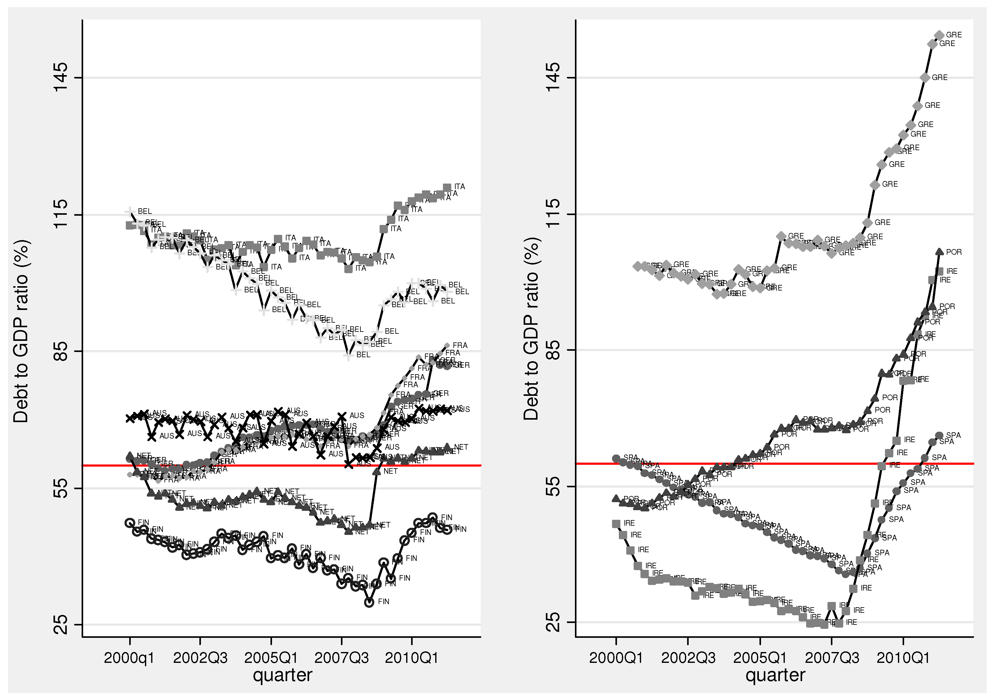
Figure 1 displays the debt-to-GDP ratios of the original 11 EMU countries. To make the graph easier to read, we split the countries between the periphery (Greece, Ireland, Portugal and Spain) and the core (the other seven countries). The red line captures the Stability and Growth Pact limit on government debt set at 60% of GDP. First, it is worth noting that, even before the financial and economic crisis of 2008, only four countries maintained debt-to-GDP ratios below the 60%-threshold: Finland, the Netherlands, Ireland and Spain. Greece, Italy and Belgium all had ratios well above the 60% threshold, averaging respectively 104%, 108% and 99%. While several countries saw their debt ratios fall before the financial crisis, these ratios increased in every country after 2008. The increase is particularly striking in the periphery countries. Between the last quarter of 2008 and early 2011, the debt-to-GDP ratio increased 57.6 percentage points in Ireland, 41.3 percentage points in Greece, 32.9 percentage points in Portugal and 25.9 percentage points in Spain. Unlike Greece, whose debt troubles stemmed from fiscal indiscipline, the rapid rise in Spanish and Irish debts originated from the private sector [25]. Following the U.S. subprime mortgage crisis, these two countries’ governments were forced to bail-out the private sector (banking systems). Portugal’s debt crisis is caused by much the same problems as Greece: overspending by the government and an overly large and bureaucratic civil service. Consequently, as shown in Figure 1, the debt-to-GDP ratios of Greece and Portugal had been rising long before the economic crisis of 2008 (especially in Portugal), whereas Spain and Ireland had been able to reduce their debt-to-GDP ratios and keep them below the 60%-threshold before they had to rescue their banking sectors.
Figure 1. Debt-to-GDP ratio in Economic and Monetary Union (EMU) countries.
Socsci 02 00318 g001
Notes: Debt data are not available for 1999. The red line captures the Stability and Growth Pact limit on government debt set at 60% of GDP.
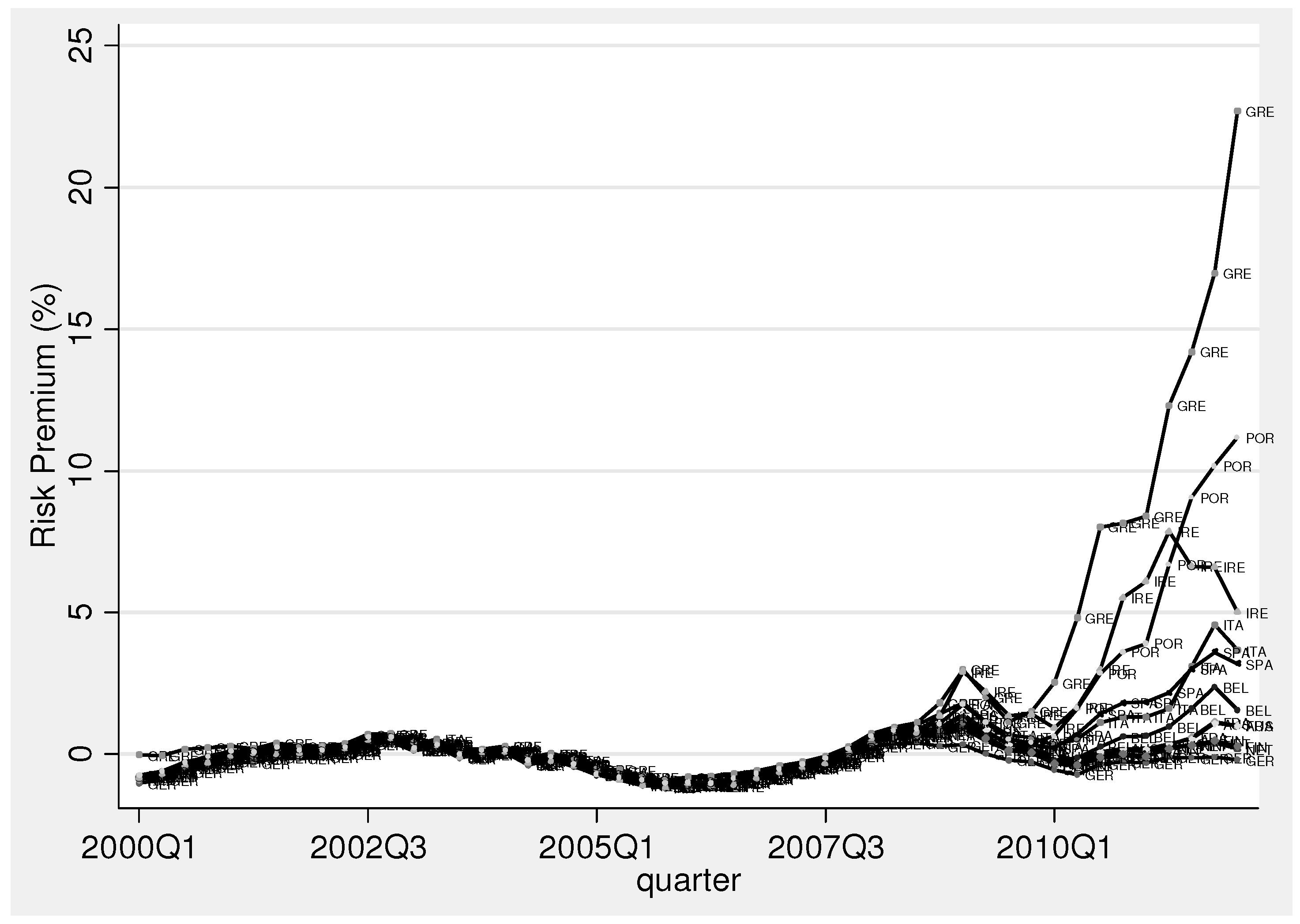
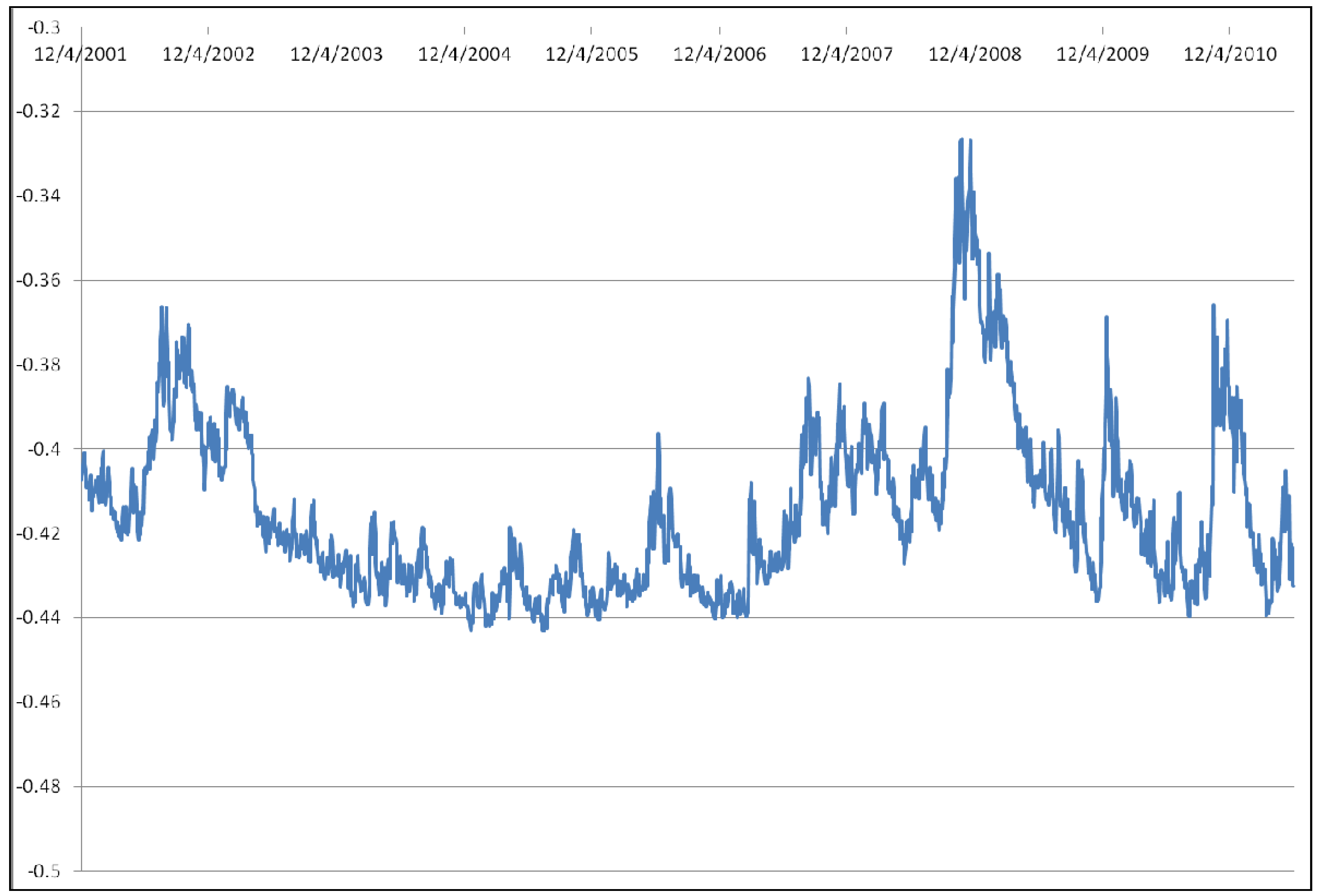
Turning now to the government-bond yield spread (Figure 2), most EMU countries enjoyed sovereign spreads with U.S. Treasury bonds close to zero and even negative (between 2005 and 2007) until the financial and economic crisis. While many countries experienced a slight increase in their sovereign spreads in 2008, the rapid increase in the risk-premia of periphery countries was initiated by the sovereign debt crisis in Greece in late 2009. These premia have continued to escalate, and reached, in the first quarter of 2012, 22.7% in Greece, 11.18% in Portugal and 3.2% in Spain. Caggiano and Greco [24] find that the correlation between sovereign spreads and debt-to-GDP ratios (especially for countries where the ratio is >100%) has increased since the financial crisis. Barrios et al. [6] find that an increase in general risk perception is more important in explaining rises in sovereign risk spreads than domestic factors. However; increases in perceived risk heighten the effect of domestic imbalances on risk-spreads during times of financial stress. The situation in Ireland is slightly different in so far as its risk premium peaked during the second quarter of 2011. The Irish government’s commitment to public-debt reduction and the ratification by Ireland of the Treaty on Stability, Coordination and Governance in the Economic and Monetary Union by referendum in May, 2012, eased Ireland’s access to funds.
Figure 2. Risk premia in EMU countries.
Socsci 02 00318 g002
Note: The risk premium is measured as the difference between a country’s ten-year bond rate and the rate on the ten-year U.S. Treasury note.
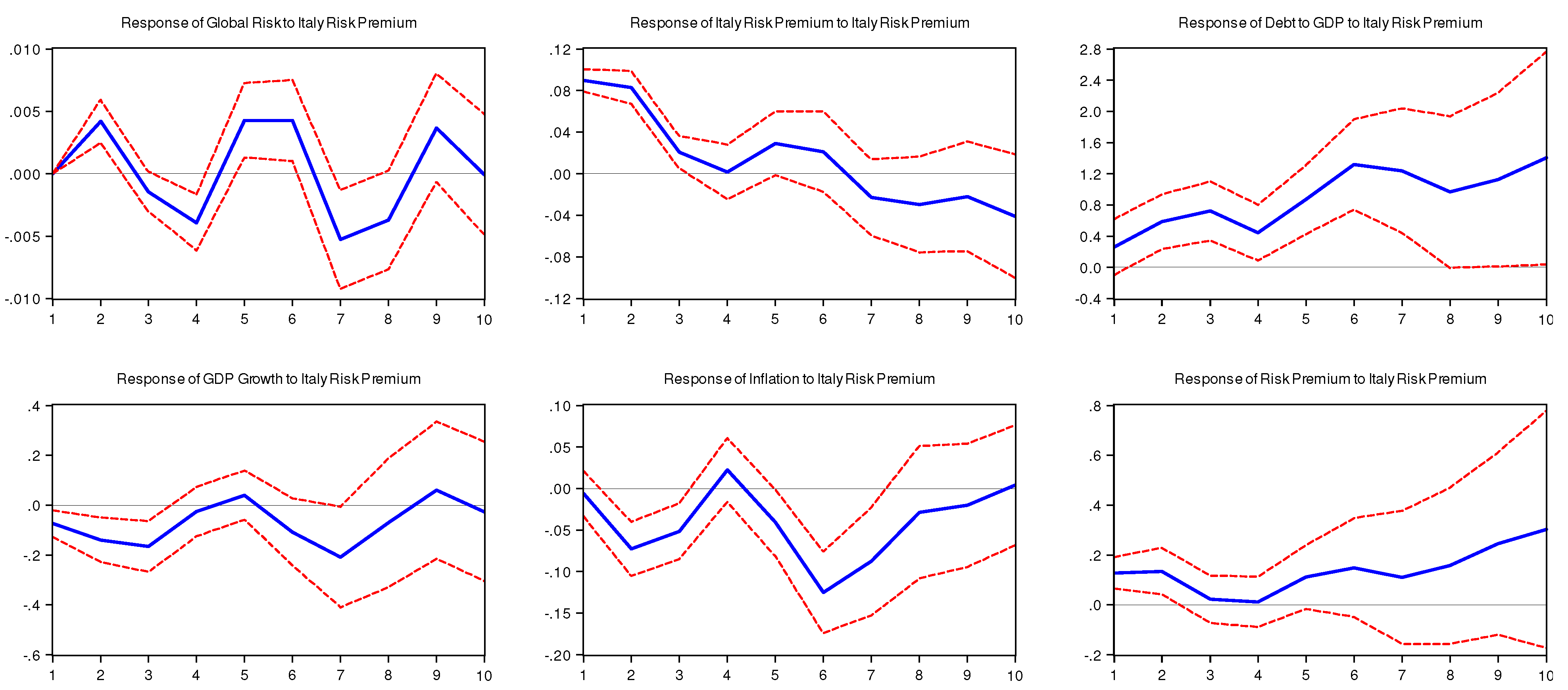
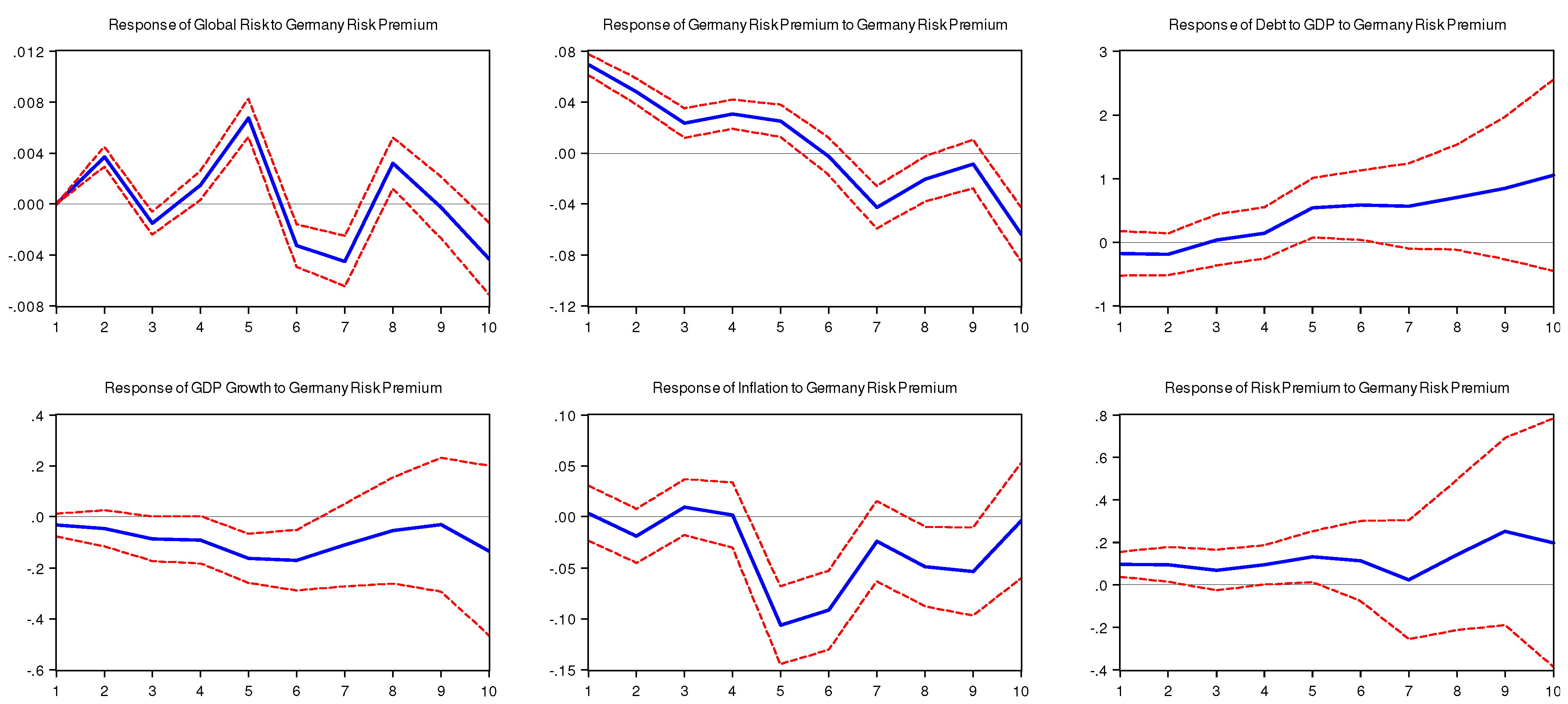
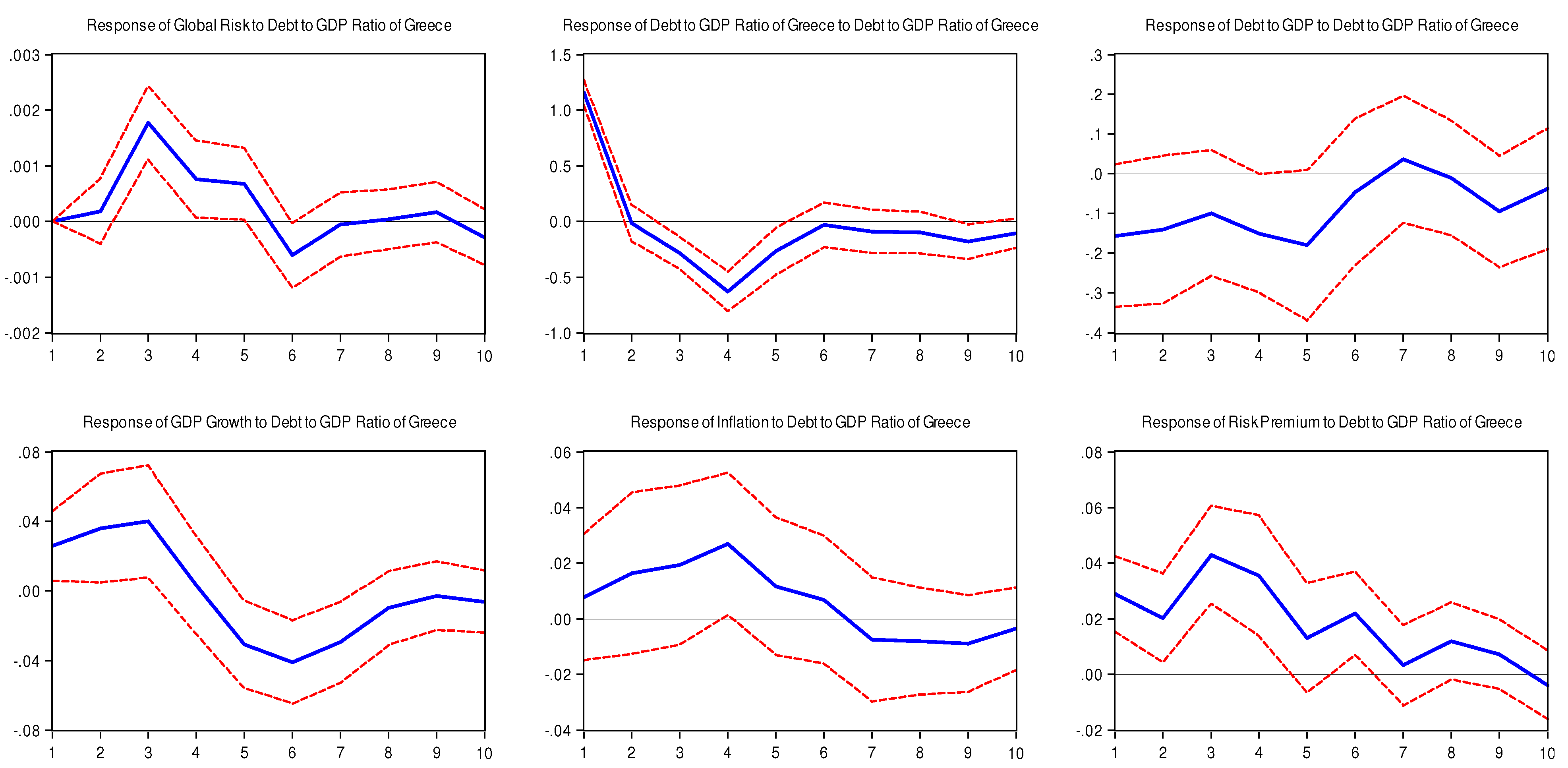
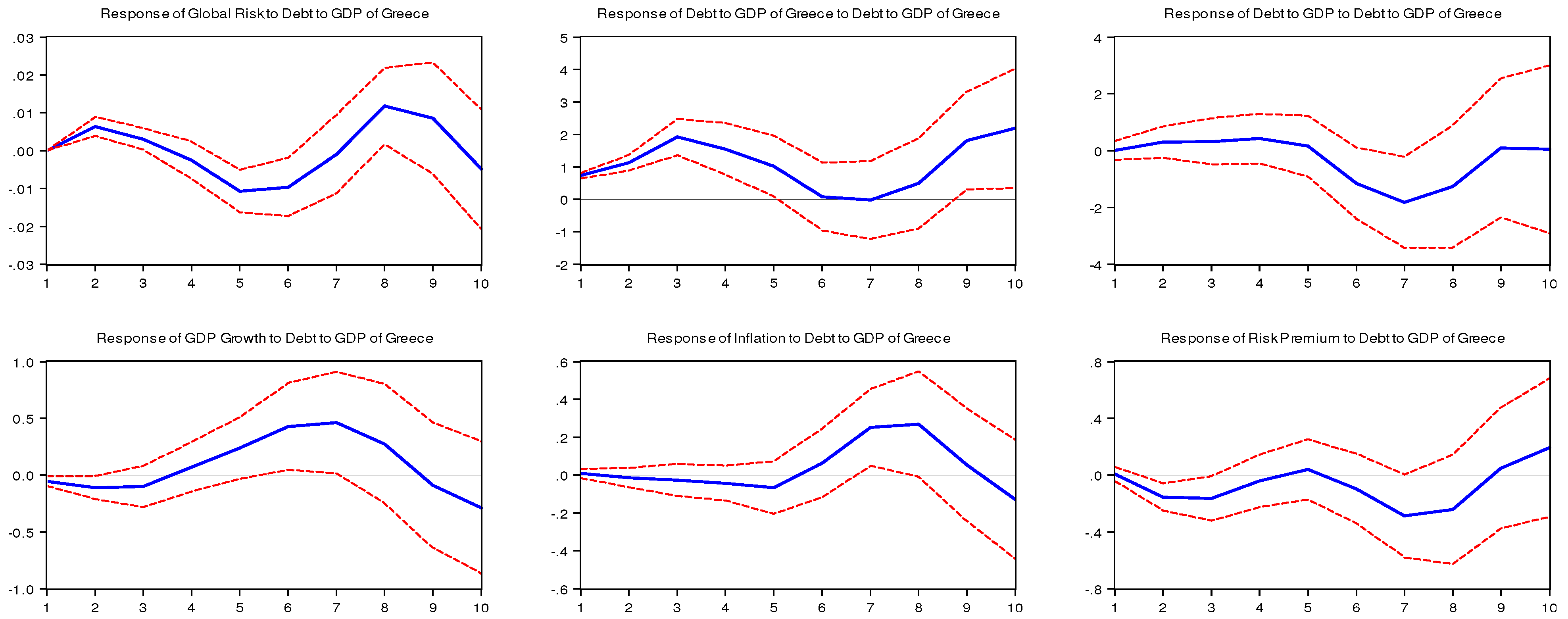
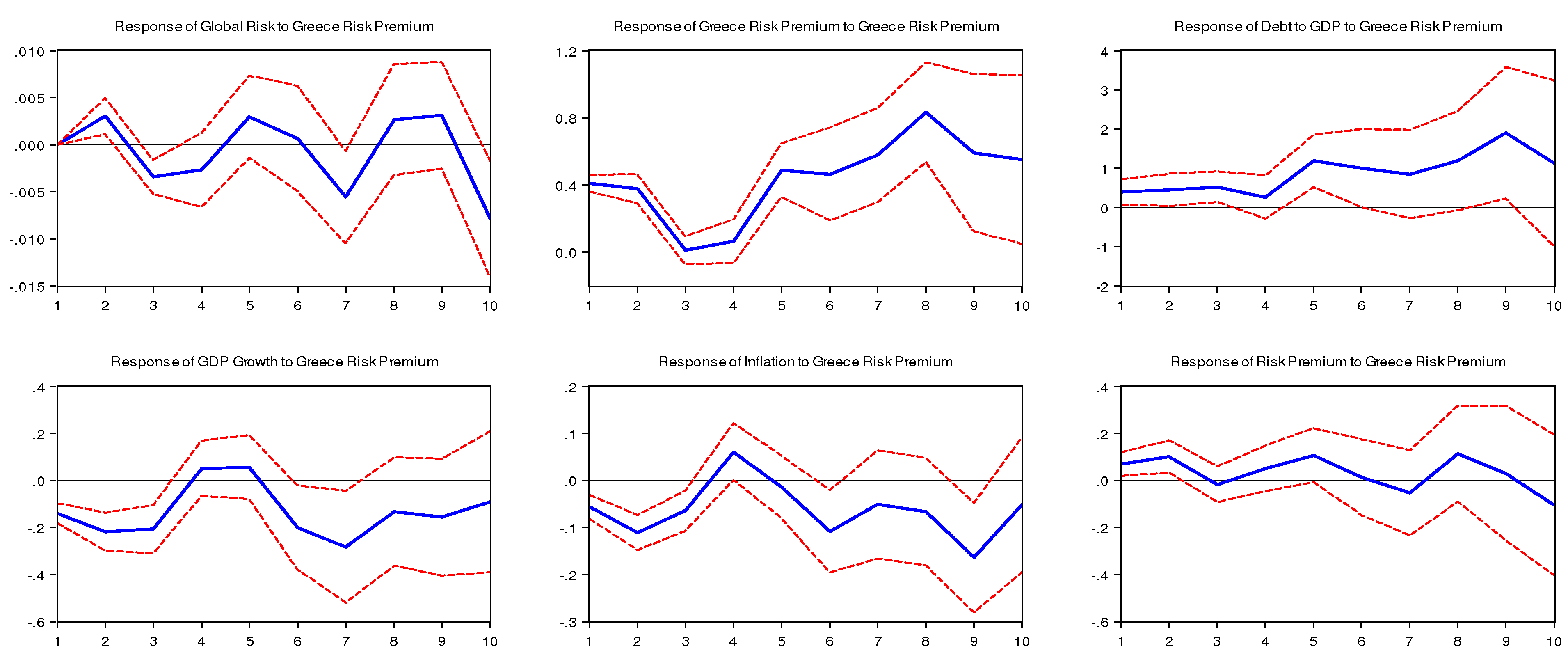
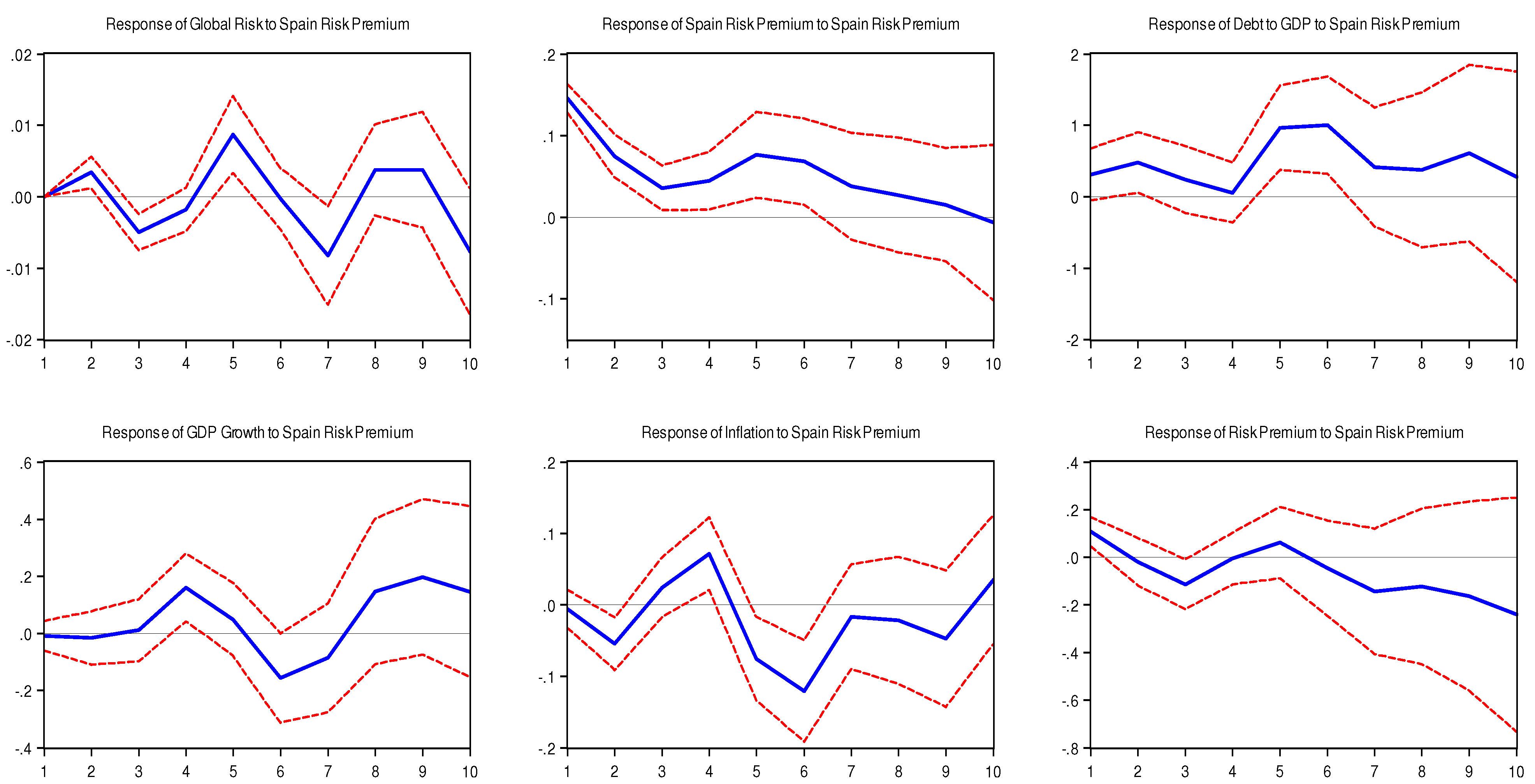
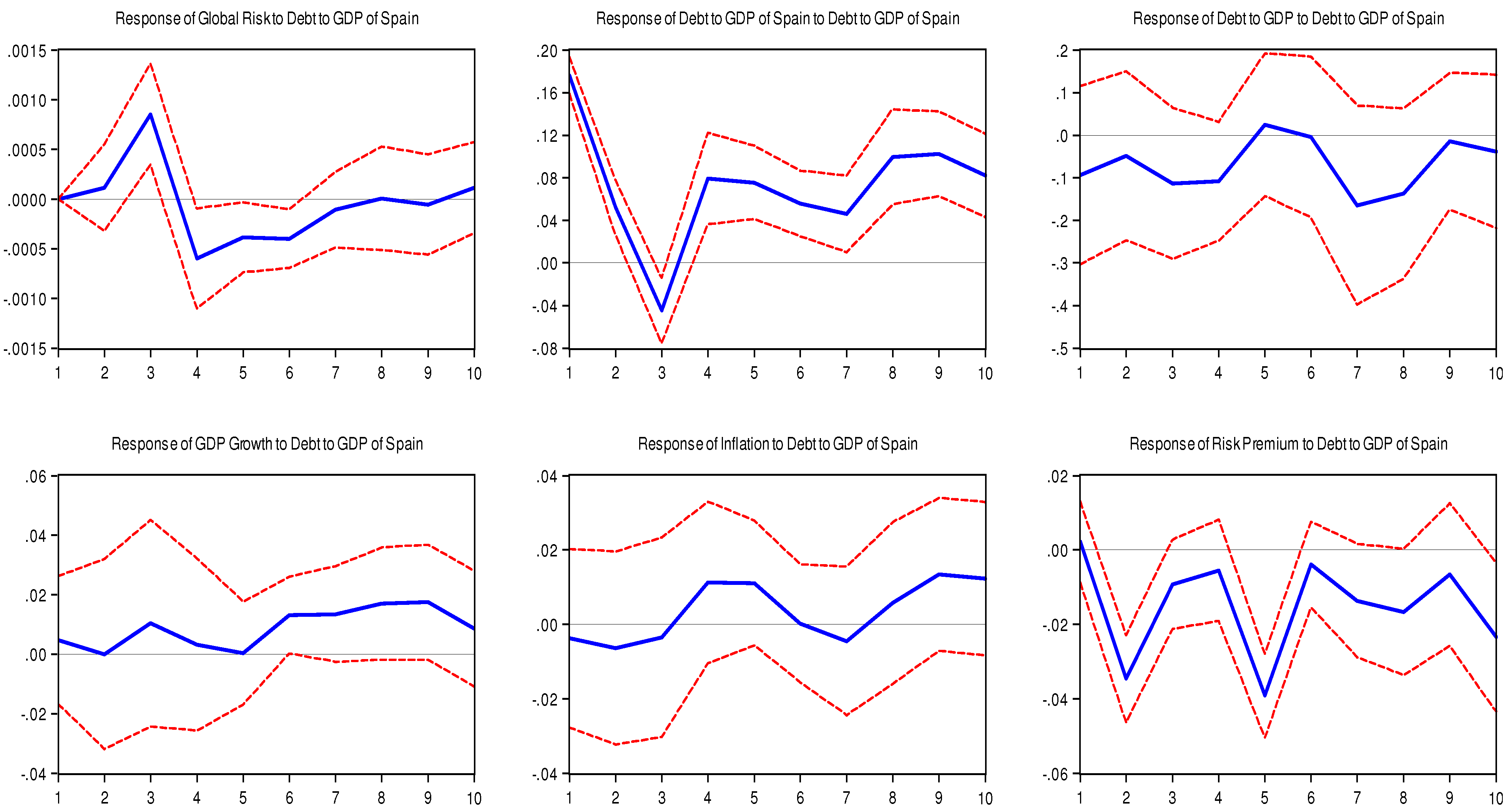
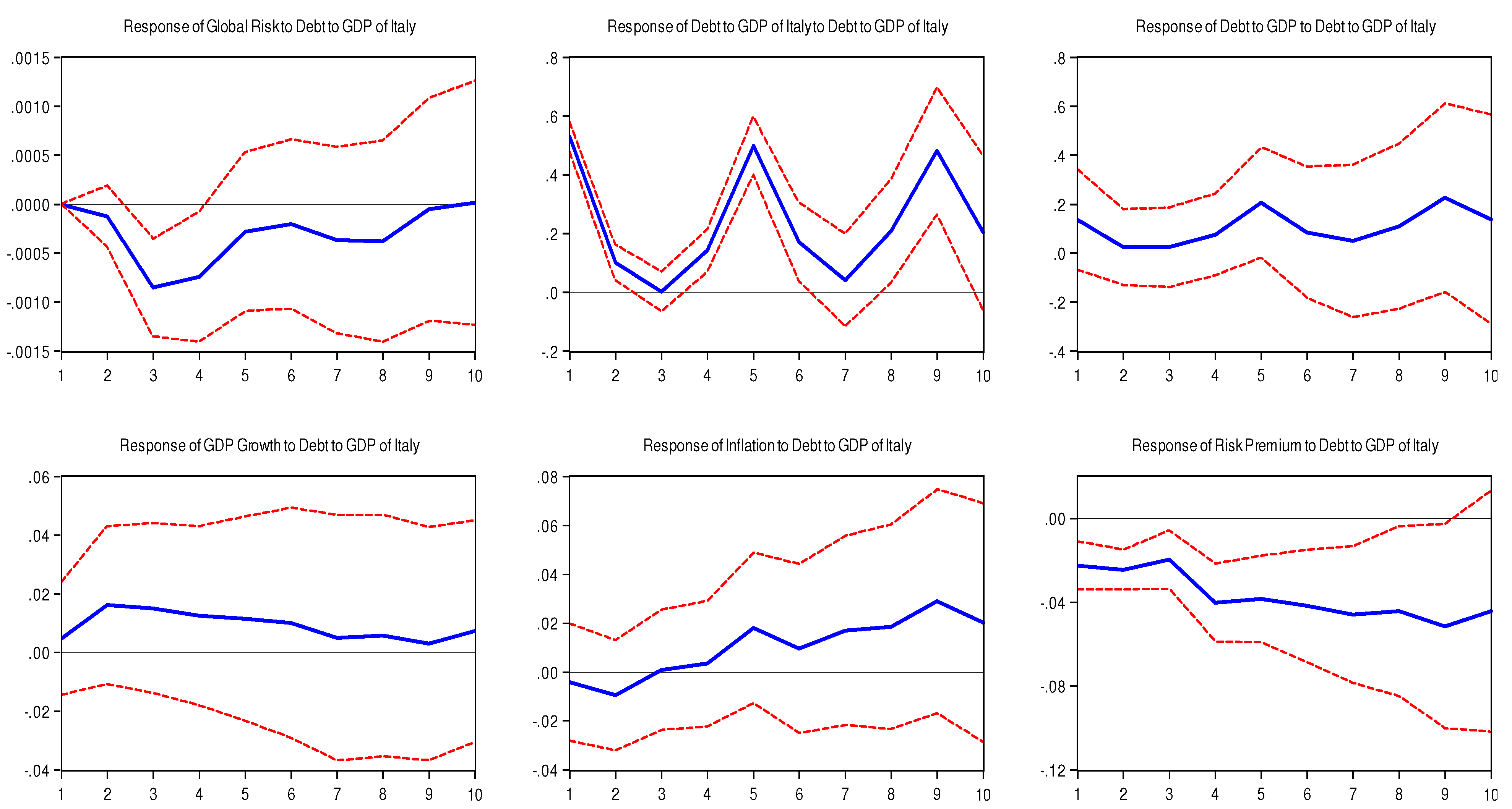
In order to assess whether the sovereign debt crisis of one particular country, such as Greece, has affected other countries’ sovereign spreads and economic outcomes, we include the Greek risk premium or its debt-to-GDP ratio in our PVAR. While several papers in the literature assume contagion would stem from Greece alone [1,
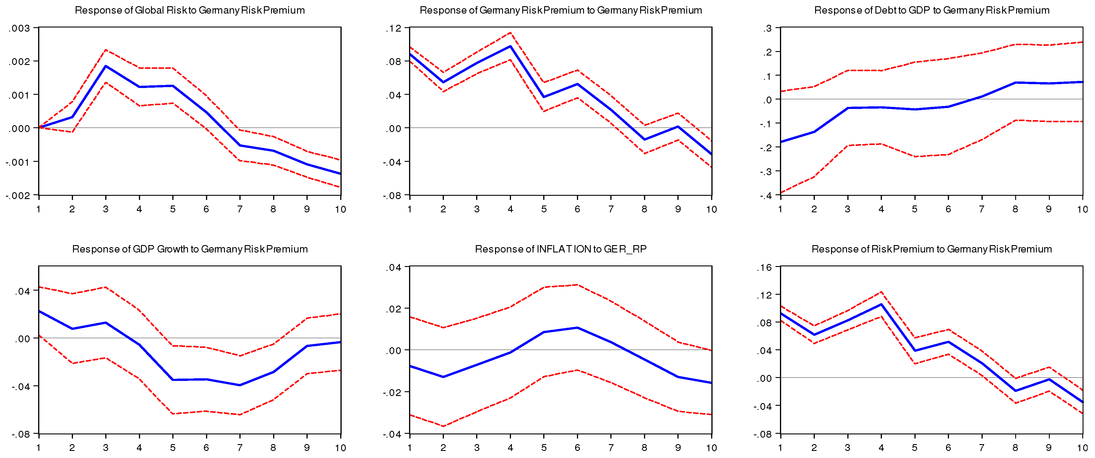
3], we also check the impact of shocks to larger economies, which have seen their sovereign spreads rise more recently, namely Italy and Spain. For comparison purposes, we also examine whether shocks to Germany (the largest economy in the EMU) induce the same type of contagion. Consequently, while our sample includes 11 EMU members, in practice, the PVARs discussed in the next section are estimated with only ten members each that are defined by exclusion of the country defining the “country-of-interest” risk premium.
Because the surge in global risk aversion is a significant factor affecting sovereign spreads [6,16,26], our model also includes a measure of global risk aversion (GRA). At times of high financial market risks, investors tend to sell high-risk government bonds and buy less risky ones, leading to higher sovereign spreads in more risky economies. Our GRA measure is based on the method proposed by Espinoza and Segoviano [27] and used by Carceres et al. [16]. The price of an asset reflects both this asset’s returns and the price that “investors are willing to pay for receiving income in ‘distressed’ states of nature.” (p. 6, [16]) The index of global risk aversion measures the market price of risk. The GRA measure is constructed using the following formula:
G R A t = ( 1 P o R t )
where P o R t is the share of the market price due to idiosyncratic risk as a fraction of the actual probability of a negative event. The GRA index captures the market’s perception of risk at every point in time. The GRA measure is exogenously given and common to all the countries included in the sample. Moreover, insofar as the market price of risk is estimated using the VIX (the Chicago Board Options Exchange Volatility Index) and the U.S. Libor- overnight indexed swap (OIS), the GRA measure also captures liquidity difficulties in financial markets. A rise in the index of global risk aversion implies an increase in global risk aversion. As shown in Figure 3, the GRA index captures the rise in global aversion observed after August, 2008, and peaking in October, 2008, after Lehman Brothers’ bankruptcy. After a gradual reduction in 2009, the index spikes again in December, 2009, when the Greek government announced that its debts had reached 300 bn euros and its budget deficit for 2009 was 12.7%, four times the level allowed by the Maastricht Treaty. The more recent increase in the last quarter of 2010 corresponds to the spread of the sovereign debt crisis to other EMU countries.
Figure 3. Index of global risk aversion.
Socsci 02 00318 g003
Note: Authors’ own calculation based on Carceres et al. [17].
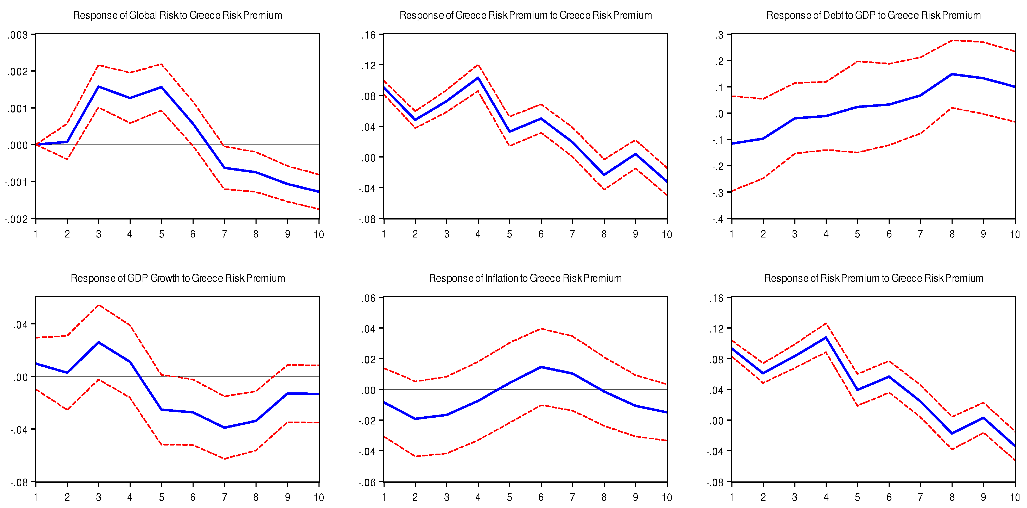
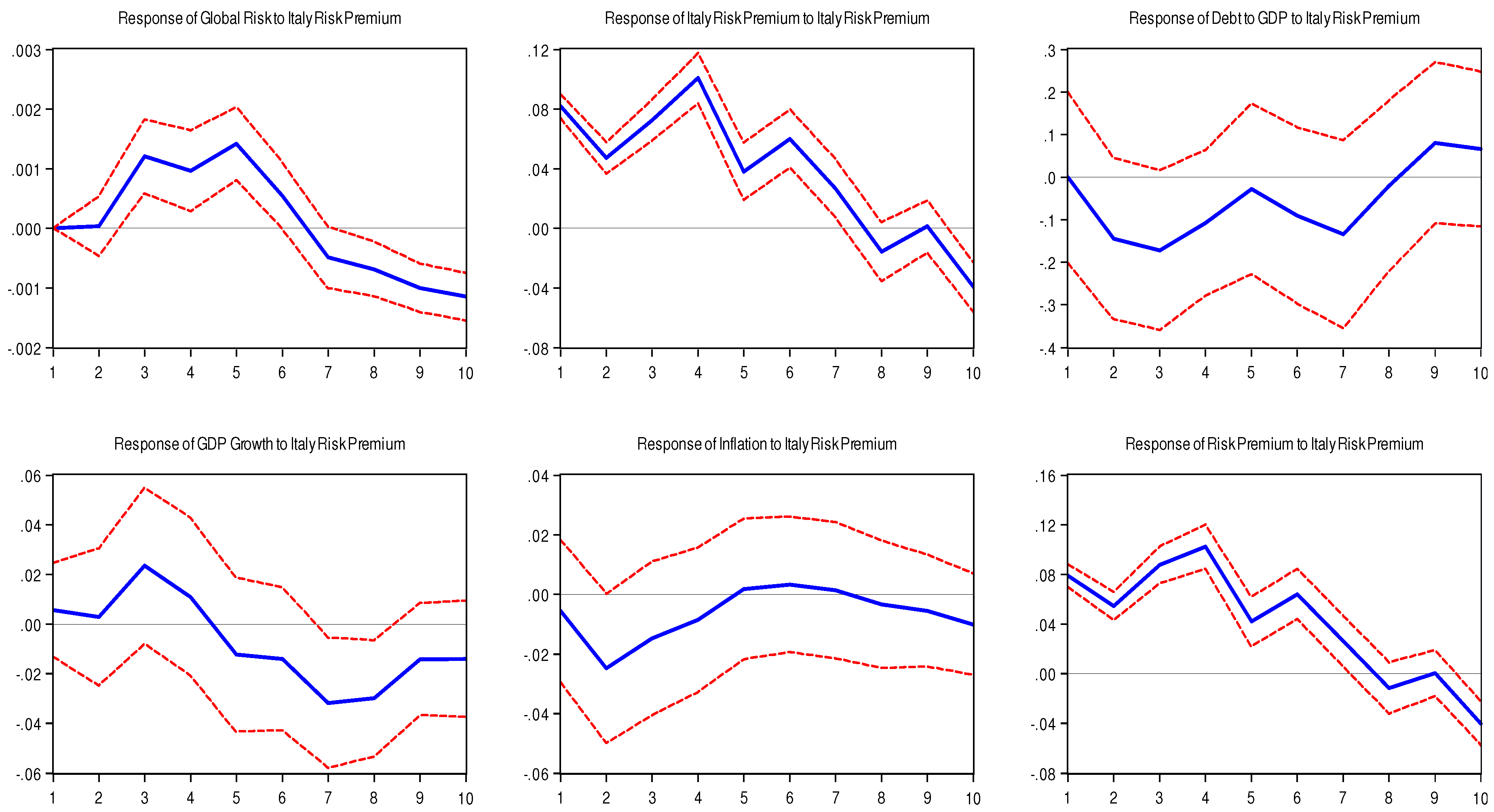
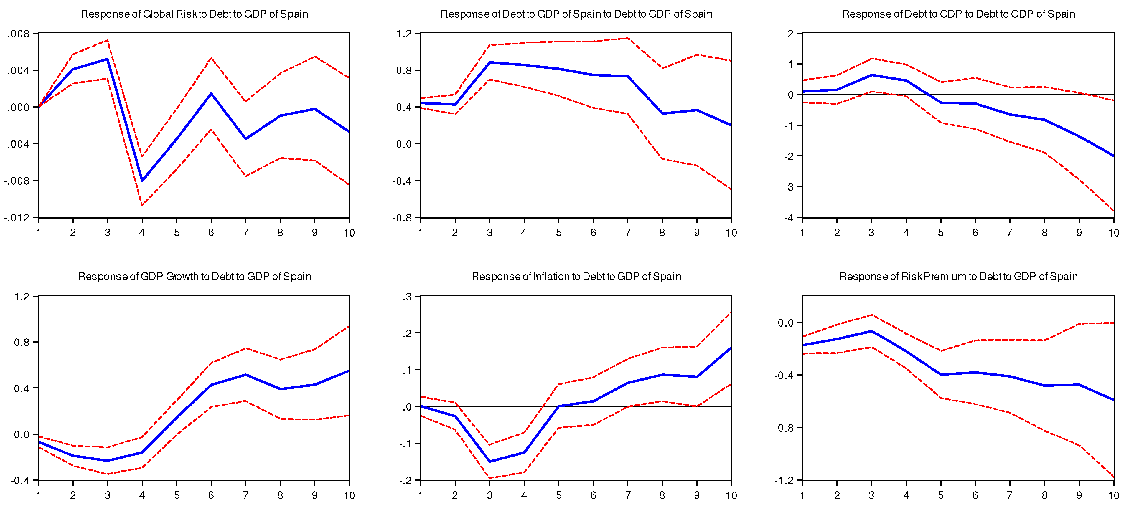
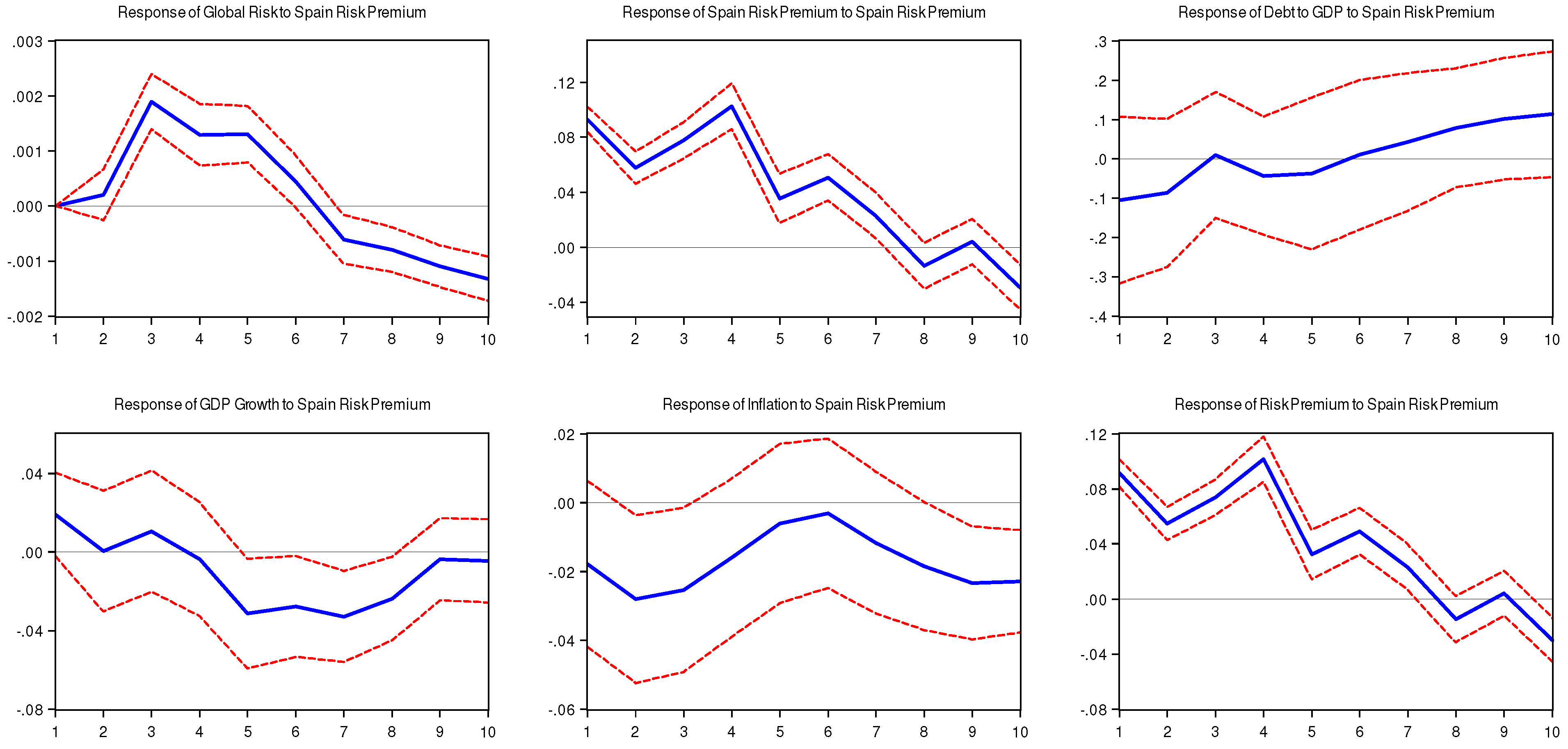
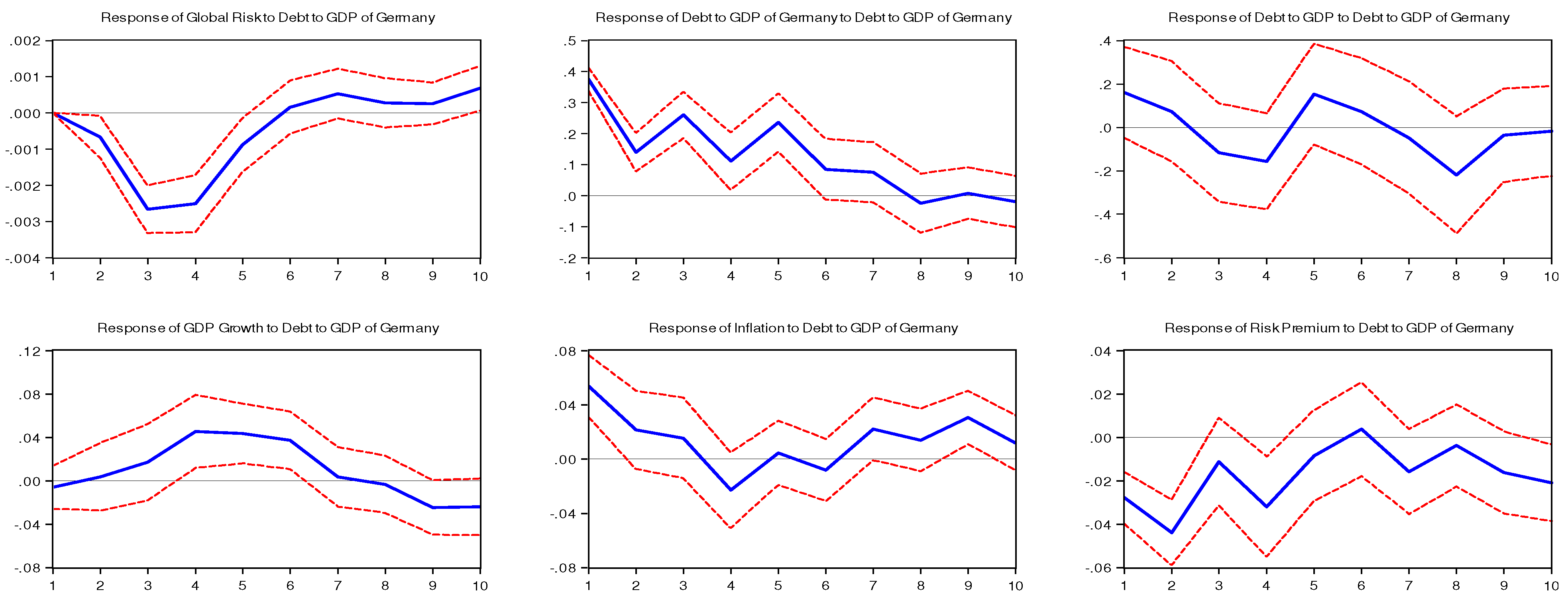
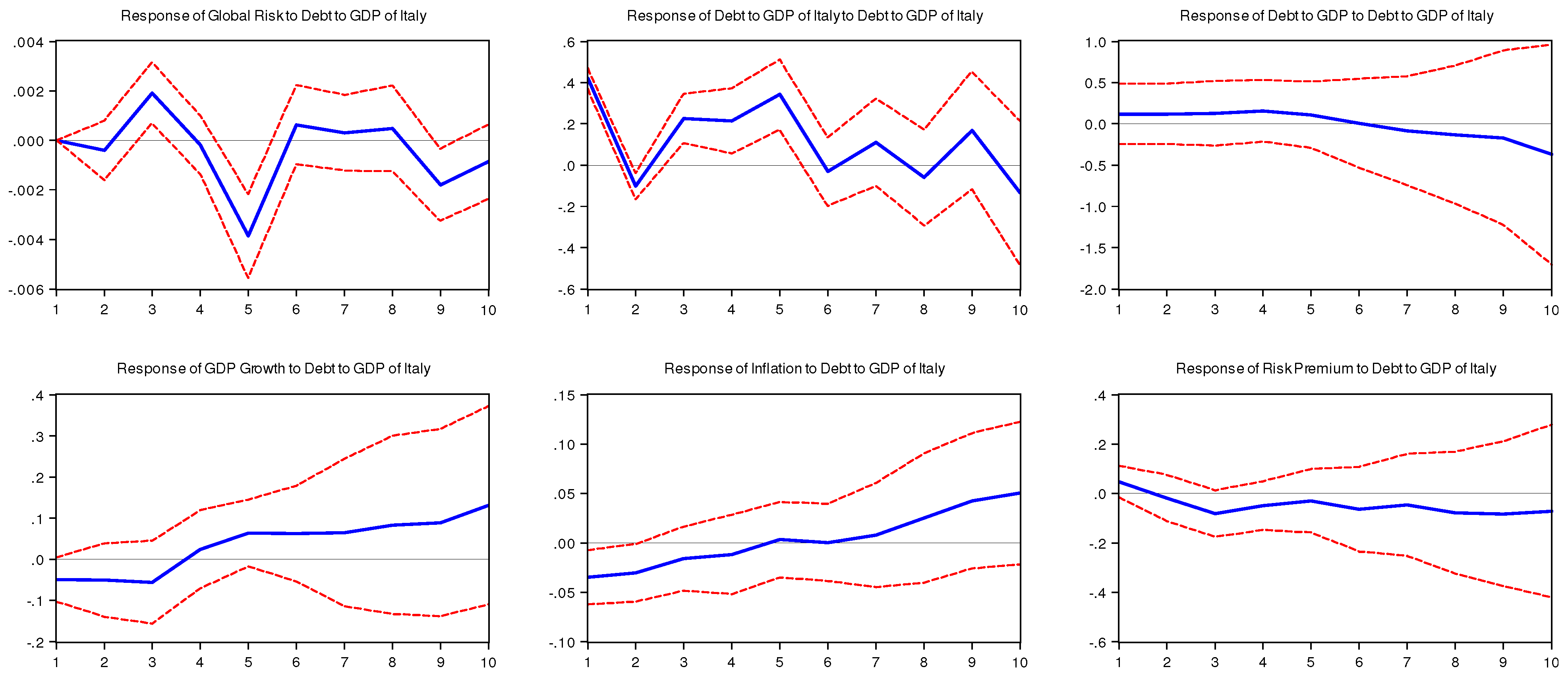
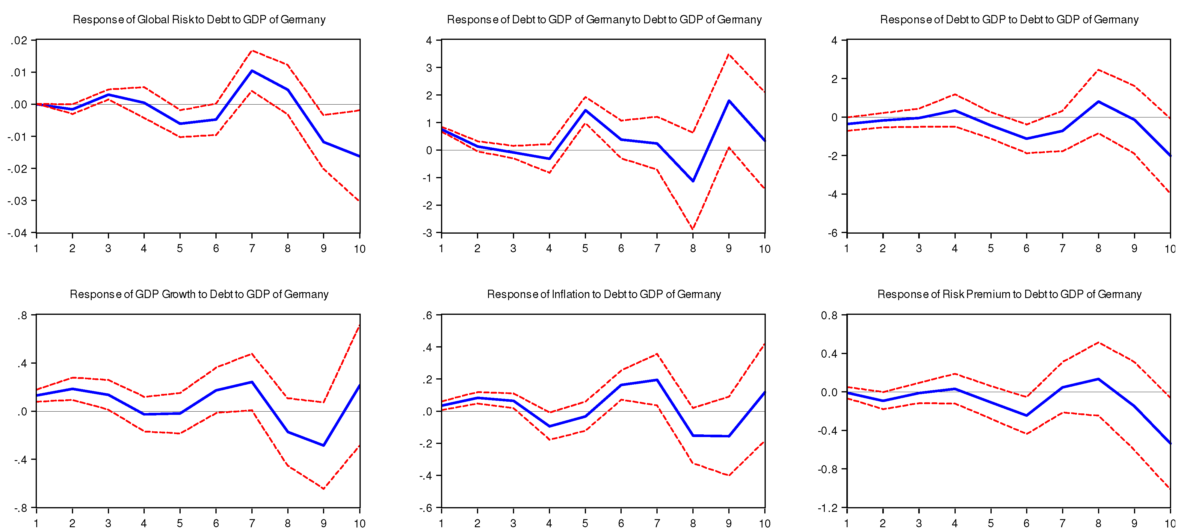
We again follow common practice and identify structural impulse response functions using recursive identification (through the Cholesky decomposition), with the variables ordered as follows: global risk aversion (GRA), “country-of-interest” risk premium, the debt-to-GDP ratio, the rate of real GDP growth, the rate of inflation and the other countries’ risk premium. The recursive order dictates that the other countries’ risk premium responds to changes in the other variables in time t. In contrast, GRA only responds to itself in time t and only with a lag to the other EMU-specific variables. After performing both selection tests and robustness checks and comparing the results at different lag lengths (see the brief discussion below for more detail), we estimate the system with four lags.
Before we discuss the results, we briefly comment on the robustness of the results we report below to alternative specification choices. For example, in our analysis, we order debt-to-GDP ahead of GDP growth based on the logic that the level of debt is not likely to respond immediately to a shock in the growth rate of GDP, but with a lag, as government budgets respond sluggishly to such changes. However, one could argue the contrary if automatic stabilizers immediately change the ratio. We considered this alternative ordering, but the change in ordering does not affect our analysis and conclusions. We attach figures for the alternative options we estimated as an appendix to our main analysis. For brevity, we include the additional results only for Greece. However, a full set of alternative results are available for Spain, Italy and Germany. Given the Appendix with figures only for Greece runs eight pages, the figures for the other three countries are available upon request, but not included here for some semblance of brevity.
Other options we considered included varying the lag length, adding a long-term interest rate for each country (in addition to the risk premium) and different transformations of some of the included variables. With respect to lag length, we considered a lag length of five and six, but the results did not change to a large degree (though, with six lags, the statistical significance of the responses is obviously diminished). After six lags, the degrees of freedom are exhausted for the pre-crisis period. For our crisis period (defined to include 2008 to 2011, which we discuss further below) the impulse response functions do not change much with five lags in the system. However, the statistical significance of the responses becomes weaker, and stretching the lag length beyond five made estimation in the short sample impossible. Estimating with shorter lag lengths did not change the inference greatly, except to make the statistical significance of the impulse response functions more pronounced.
We also estimated the debt-to-GDP ratio in the first differences and GDP in log levels (instead of a growth rate). These alternatives did not change the results substantially, nor did adding the ten year rate for each country (which might be included if one believes the level of a country’s long-term rate has a distinct effect on the system from the risk premium). Lastly, while we focus on the pre-crisis sample versus crisis sample for comparison, the Appendix also reports the results for the full sample period. Overall, changes to the PVAR model along these various lines did not affect our inference to a large degree, especially when comparing the pre-crisis period to the crisis period. Of course, as more data become available over time, a researcher will be less bound by the restrictions we face here in analyzing the crisis period, but we feel the analysis below offers a useful understanding of the spread of financial pressure across the EU, one that is relatively robust to typical variations in PVAR estimation.

3. Results

3.1. Shock to a Country’s Risk Premium

In the first set of impulse response functions below (Figure 4), we report results from a PVAR estimated with Greece’s risk premium to gauge the effect of a one positive standard deviation shock to that country’s risk premium on the remaining ten countries in the sample (so, Greek data are excluded from the remaining variables). The motivation for such a strategy is to isolate the effect of a change in one country’s risk premium on the other members of the EMU. We estimate the PVAR system, in turn, for shocks originating in Spain, Italy and Germany, as we do for Greece (reported in Figure 5, Figure 6 and Figure 7). Finally, since we estimate with a long panel (n = 10 and t = 39), we control for country fixed-effects using dummy variables.5 Based on limitations to the global risk aversion variable, the sample spans the first-quarter of 2001 through the second-quarter of 2011. We compute the responses over a 10-quarter horizon. For inference, we report standard asymptotic standard errors for the impulse response functions.
Below, we discuss, first, the responses displayed in Figure 4, Figure 5, Figure 6 and Figure 7 for the pre-crisis period (2001–2007). Then, we conduct the same exercise, but for the crisis period (2008–2011), to check for evidence of contagion effects. Later, we also analyze the response of the system variables to a shock to the debt-to-GDP ratio, again for the pre-crisis and crisis periods.6
Figure 4. Pre-crisis response of EMU countries to a shock to the Greece risk premium: 2001–2007.
Socsci 02 00318 g004
Notes: Impulse response functions estimated from six-variable vector autoregression (VAR), controlling for country-fixed effects, and with identification achieved through Cholesky decomposition (see the text for ordering). Shock is defined as a Cholesky one-standard deviation. Dotted lines show the plus or minus two-standard error bands. Horizon measured in quarters. The sample spans the fourth quarter of 2001 through the fourth quarter of 2007. See the text for additional details.
Figure 5. Pre-crisis response of EMU countries to a shock to Spain’s risk premium: 2001–2007.
Socsci 02 00318 g005
Notes: Dotted lines show the plus or minus two-standard error bands. The horizon is measured in quarters. See the notes to previous figures for additional details.
Splitting the sample at the beginning of 2008 is motivated primarily by the notable change in Greece’s risk premium at some point in 2008 (displayed in Figure 2). In addition, as the discussion surrounding Figure 1, Figure 2 and Figure 3 suggest, anecdotally, the “crisis” began in full earnest in 2008. To check this notion statistically, we apply Bai and Perron’s [29,30] structural break methodology to the risk premium for each country in our sample. Bai and Perron [29,30] provide a method for estimating the existence of unknown (a priori) breaks and significance tests for any found break date. We find evidence of a statistically significant break date in Greece’s risk premium in the fourth quarter of 2008. For Spain and Italy, we find a statistically significant break in the fourth quarter of 2007. For the eight other countries in our sample, a break occurs in seven of them at some point in late 2007 or 2008.7 Hence, we feel that 2008 is an appropriate point to split our sample into the pre-crisis and crisis periods.

3.1.1. Pre-Crisis Period (2001–2007)

As shown in Figure 2, EMU countries enjoyed similar, low sovereign spreads (the standard deviation for this period is 0.5% or 50 basis-points). Consequently, shocks8 to different countries’ sovereign spreads yield quite a similar response from the rest of the EMU. First, as shown in Figure 4, Figure 5, Figure 6 and Figure 7, debt-to-GDP ratios in other EMU countries are not significantly affected by a shock to sovereign spreads. We only observe an economic slowdown between the fifth and eight quarters following the shock. Shocks to Greece, Spain, Italy and Germany’s risk premia trigger a similar response from the risk premia of other EMU countries. A worsening of these four countries’ risk premium increases remaining EMU countries’ sovereign spreads by 8–9 basis-points the first quarter and up to 10 basis-points at the end of the first year. Then, the effect progressively diminishes, until it becomes statistically insignificant by the end of the 10-quarter time horizon. We also find a similar response from the GRA index, which rises 0.2 basis-points after the risk premium shock.
Figure 6. Pre-crisis response of EMU countries to a shock to Italy’s risk premium: 2001–2007.
Socsci 02 00318 g006
Notes: Dotted lines show the plus or minus two-standard error bands. The horizon is measured in quarters. See the notes to previous figures for additional details.
Figure 7. Pre-crisis response of EMU countries to a shock to the German risk premium: 2001–2007.
Socsci 02 00318 g007
Notes: Dotted lines show the plus or minus two-standard error bands. The horizon is measured in quarters. See the notes to previous figures for additional details.

3.1.2. Crisis period (2008–2011)

Unlike in the pre-crisis period, the response of EMU economies to risk-premium shocks from the four countries studied in this paper are not identical. This is partly due to differences in the magnitude of the shocks (i.e., standard deviations in the risk premium variable): the standard deviation for Greece’s sovereign spread (659 basis-points) is more than 20 times larger than the standard deviation of the German sovereign spread (33 basis-points).
Figure 8 shows the responses of the six variables included in our PVAR model to a one positive standard deviation shock to the risk premium of Greece (equal to 659 basis-points). A worsening of the Greek risk premium increases the other EMU countries’ sovereign spreads by 10 basis-points in the first two quarters. This slight rise in risk premia can be explained by a comparable rise in global risk aversion in the first two quarters after the shock to Greece’s sovereign spread. The initial negative impact of the Greek risk premium shock on economic growth is consistent with rising debt-financing costs, as well as the rising debt-to-GDP ratio, which increases by 50 basis-points after one year, up to 200 basis-points by the end of the simulation span.
Figure 8. Response of EMU countries to a shock to Greece’s risk premium during the crisis: 2008–2011.
Socsci 02 00318 g008
Notes: Impulse response functions estimated from six-variable VAR, controlling for country-fixed effects, and with identification achieved through Cholesky decomposition (see the text for ordering). Shock is defined as a Cholesky one-standard deviation. Dotted lines show the plus or minus two-standard error bands. The horizon is measured in quarters. The sample spans the first quarter of 2008 through the second quarter of 2011. See the text for additional details.
When the sovereign debt crisis originates from a larger economy, such as Spain (Figure 9) or Italy (Figure 10), the impact on the other EMU countries is more severe, since a much smaller shock to Spain’s risk premium (+107 basis-points, i.e., less than a fifth of the Greek risk premium shock) or Italy’s risk premium (+117 basis-points, i.e., similar to the shock to Spain’s risk premium) also increases the risk premium of other countries by 10 basis-points in the first two quarters. For both Spain and Italy, this rise in borrowing costs triggers an increase in debt-to-GDP ratios by almost 100 basis-points after five quarters. The response then becomes statistically insignificant for Spain, but remains significant for Italy.
Figure 9. Response of EMU countries to a shock to Spain’s risk premium during the crisis: 2008–2011.
Socsci 02 00318 g009
Notes: Dotted lines show the plus or minus two-standard error bands. The horizon is measured in quarters. See the notes to previous figures for additional details.
Figure 10. Response of EMU countries to a shock to Italy’s risk premium during the crisis: 2008–2011.
Socsci 02 00318 g010
Notes: Dotted lines show the plus or minus two-standard error bands. The horizon is measured in quarters. See the notes to previous figures for additional details.
What if the shock (again, one positive standard deviation, +33 basis-points) originated from the largest EMU economy, which also offers AAA-rated assets, namely Germany? This scenario is investigated in Figure 11. We find that other EMU countries see their risk premia increase by 10 basis-points over the first year, as Germany loses some of its appeal as a safe haven for investors, and this effect spills over to other EMU economies. Debt-to-GDP ratios in other EMU countries do not increase as in the other scenarios considered earlier9. However, because Germany is a bigger player in the world economy, the shock to Germany’s risk premium (a twentieth of the shock to Greece’s risk premium) induces a larger and slightly more persistent drop in the other countries’ economic growth, and an increase in the global risk aversion index. This phenomenon might explain why other EMU countries would see their risk premia initially rise, as investors’ seek refuge in U.S. Treasury notes.
Figure 11. Response of EMU countries to a shock to Germany’s risk premium during the crisis: 2008–2011.
Socsci 02 00318 g011
Notes: Dotted lines show the plus or minus two-standard error bands. The horizon is measured in quarters. See the notes to previous figures for additional details.
Overall, these simulations provide some evidence of contagion within the EMU, as shocks to sovereign spreads from periphery countries trigger large increases in debt-to-GDP ratios in other countries. There is, however, no clear sign of contagion to other countries’ risk premia, as these spreads increase only very temporarily during the crisis period, despite much larger shocks to the spreads of Greece, Spain and Italy.

3.2. Shock to a Country’s Debt-to-GDP Ratio

To further investigate the presence of contagion of fiscal imbalances among EMU countries, we show in Figure 12, Figure 13, Figure 14 and Figure 15 the responses to a one positive-standard-deviation shock to the debt-to-GDP ratio of Greece, Spain, Italy and Germany in the pre-crisis period (2001–2007). We then contrast these responses with those obtained for the crisis period (2008–2011).

3.2.1. Pre-Crisis Period (2001–2007)

Because shocks to countries’ debt-to-GDP ratios trigger different responses, we discuss them individually.
Figure 12. Pre-crisis response of EMU countries to a shock to the Greek debt-to-GDP ratio: 2001–2007.
Socsci 02 00318 g012
Notes: Impulse response functions estimated from six-variable VAR, controlling for country-fixed effects, and with identification achieved through Cholesky decomposition (see the text for ordering). Shock is defined as a Cholesky one-standard deviation. Dotted lines show the plus or minus two-standard error bands. The horizon is measured in quarters. The sample spans the fourth quarter of 2001 through the fourth quarter of 2007. See the text for additional details.
Figure 13. Pre-crisis response of EMU countries to a shock to Spanish debt-to-GDP ratio: 2001–2007.
Socsci 02 00318 g013
Notes: Dotted lines show the plus or minus two-standard error bands. The horizon is measured in quarters. See the notes to previous figures for additional details.
Figure 14. Pre-crisis response of EMU countries to a shock to the Italian debt-to-GDP ratio: 2001–2007.
Socsci 02 00318 g014
Notes: Dotted lines show the plus or minus two-standard error bands. The horizon is measured in quarters. See the notes to previous figures for additional details.
Figure 15. Pre-crisis response of EMU countries to a shock to the German debt-to-GDP ratio: 2001–2007.
Socsci 02 00318 g015
Notes: Dotted lines show the plus or minus two-standard error bands. The horizon is measured in quarters. See the notes to previous figures for additional details.
Prior to the crisis (Figure 12, Figure 13, Figure 14 and Figure 15), we find no evidence of contagion between debt-to-GDP ratios. However, shocks to countries’ debt-to-GDP ratios trigger different responses in other countries’ risk premia. On the one hand, a shock to Greece (Figure 12), a 390-basis-points increase in the Greek debt-to-GDP ratio, triggers a rise in global risk aversion and in sovereign spreads initially by three basis-points and by four basis-points by the third quarter. On the other hand, when the debt-to-GDP ratio shock originates from one of the other three countries, other EMU countries see their risk premia decrease by around four basis-points. The decreasing borrowing costs indicate that other countries benefit from flight-to-quality. In the case of Germany (Figure 15), the fall in other countries’ risk premia is consistent with a “liquidity effect” (also found in [9]) in which the overall level of risk falls when a country, viewed as less risky by investors, issues more debt, causing a fall in the other countries’ risk premia. This liquidity effect could also explain the initial fall in the GRA index.
With the exception of Italy, a rise in the debt-to-GDP ratio usually stimulates economic growth in other countries, as additional spending by these governments increases aggregate demand in the Eurozone. Perhaps the rise in debt-to-GDP in Italy is associated with structural problems (such as tax collection problems, lack of competitiveness), which have undermined economic growth in Italy since the 1990s. Finally, given the size of the German economy in the Eurozone, an increase in the German debt-to-GDP ratio has a stronger positive effect on economic growth (+4 basis-points at the end of the first year) in other countries.

3.2.2. Crisis Period (2008–2011)

A large shock to the Greek debt-to-GDP ratio (1,550-basis-point increase) triggers very few changes in other countries’ responses (Figure 16). Initially, countries see their risk premia fall slightly, as a consequence of capital flight from Greece (and the rest of the world, since the GRA index increases slightly in the second quarter). By the sixth quarter, economic growth increases and, subsequently, the debt-to-GDP ratio in other countries falls while global risk aversion falls.
Figure 16. Response of EMU countries to a shock to Greece’s debt-to-GDP ratio during the crisis: 2008–2011.
Socsci 02 00318 g016
Notes: Dotted lines show the plus or minus two-standard error bands. The sample spans the first quarter of 2008 through the second quarter of 2011. The horizon is measured in quarters. See the notes to previous figures for additional details.
When the debt-to-GDP ratio of a larger periphery country, such as Spain (Figure 17), increases by one standard deviation (1,080 basis-points), the remaining countries in the EMU see their debt-to-GDP ratios decrease by 200 basis-points at the end of the simulation horizon, probably due to a rise in economic growth and a decline in risk premia following the 5th quarter. The risk premia fall initially by 20 basis-points and, then, by 60 basis-points ten quarters later. We observe the same capital flight from Spain as in the pre-crisis period; however, the responses are stronger (even accounting for the larger standard deviation here). This latter effect might be due to the negative response of economic growth in the first year.
Figure 17. Response of EMU countries to a shock to Spain’s debt-to-GDP ratio during the crisis: 2008–2011.
Socsci 02 00318 g017
Notes: Dotted lines show the plus or minus two-standard error bands. The horizon is measured in quarters. See the notes to previous figures for additional details.
A shock to the debt ratio of highly-indebted Italy (Figure 18) triggers no statistically significant response from the other EMU economies during the crisis period, possibly because Italy is considered “too big to fail” and the European Central Bank (ECB) will intervene. The ECB announced on August 7th, 2011, that it would buy Spanish and Italian debt to stem contagion.
Figure 18. Response of EMU countries to a shock to Italy’s debt-to-GDP ratio during the crisis: 2008–2011.
Socsci 02 00318 g018
Notes: Dotted lines show the plus or minus two-standard error bands. The horizon is measured in quarters. See the notes to previous figures for additional details.
As shown in Figure 19, a shock to Germany’s debt-to-GDP ratio (+610 basis-points) triggers a set of responses similar to those obtained for Spain. After an initial limited response, a worsening of the German debt-to-GDP ratio leads to a decline in other EMU countries’ debt-to-GDP ratios by 100 basis-points the 6th quarter. Sovereign spreads also decrease slightly in the first year and continue to decline around the 6th quarter (approximately 20 basis-points). We therefore observe the same liquidity effect as in the pre-crisis period, but with a larger magnitude. Countries might also benefit from a drop in the GRA index. Finally, a larger German debt level seems to stimulate aggregate demand in neighboring countries, as economic growth accelerates during the first three quarters following the shock.
Figure 19. Response of EMU countries to a shock to Germany’s debt-to-GDP ratio during the crisis: 2008–2011.
Socsci 02 00318 g019
Notes: Dotted lines show the plus or minus two-standard error bands. The horizon is measured in quarters. See the notes to previous figures for additional details.

4. Conclusions

In this paper, we implement a panel-VAR (PVAR) model for 11 EMU countries to examine the extent that a rise in a country’s bond-yield spreads or debt-to-GDP ratio affects the other EMU countries’ fiscal and macroeconomic outcomes. Using quarterly data for the 2000–2011 period, we find some evidence of interdependence and contagion within the EMU during the 2008–2011 period. Our estimations suggest that in the pre-crisis period, an increase in one country’s sovereign spread leads to an increase in the other countries’ borrowing costs and sovereign spreads, but does not affect their debt-to-GDP ratios. After 2008, the same shock to sovereign spread has a large effect on the countries’ debt-to-GDP ratios, if the shock stems from Greece or Spain. This suggests the existence of contagion. In the case of a shock to Germany’s sovereign spread, however, other countries barely see their borrowing costs rise, as Germany loses some of its appeal as a safe haven for investors.
When the shocks affect debt-to-GDP ratios, we do not find evidence of contagion, but whether the shock improves or worsens the other EMU economies depends on the debt level of the country “shocked”. If Germany or Spain’s debt-to-GDP ratios increase, other countries benefit from a liquidity effect and see their sovereign spreads and borrowing costs decrease. If the shock originates from Greece or Italy, then we observe no significant response in other countries. As pointed out by Caporale and Girardi [9], these contrasting results suggest that financial markets are able to discriminate among different debt-issuers. Moreover, we agree with these authors’ conclusion that the crowding-out effects of higher debt from Italy and Greece provides support for some fiscal discipline. Sound fiscal policies are indeed essential to the smooth functioning of the EMU.
To better distinguish between economic interdependence and contagion, further research would benefit from using a panel-vector error correction model, whereby the short-term dynamics would capture the possible contagion and the long-term coefficients would capture economic interdependence.

Conflicts of Interest

The authors declare no conflict of interest.

References and Notes

  1. Vitor Constancio. “Contagion and the European Debt Crisis.” Banque de France Financial Stability Review no. 16. , 2012, 109–21. [Google Scholar]
  2. Kristin Forbes. “The Big "C": Identifying contagion.” NBER Working Paper. 2012, no. 18465. [Google Scholar]
  3. Sebastian Missio, and Sebastian Watzka. “Financial Contagion and the European Debt Crisis.” CESifo Working Paper. 2011, no. 3554. [Google Scholar]
  4. Roberto De Santis. “The Euro Area Sovereign Debt Crisis. Safe Haven, Credit Rating Agencies and the Spread of the Fever from Greece, Ireland and Portugal.” ECB Working Paper. 2012, no. 1419. [Google Scholar]
  5. Sandra Eickmeier, and Tim Ng. “How do Credit Supply Shocks Propagate Internationally? A GVAR Approach.” Centre for Economic Policy Research Discussion Paper Series. 2011, no. 8720. [Google Scholar]
  6. Salvador Barrios, Per Iversen, Magdalena Lewandowska, and Ralph Setzer. “Determinants of intra-euro area government bond spreads during the financial crisis.” European Commission Directorate-General for Economic and Financial Affairs, Economic Papers. November 2009, no. 388. [Google Scholar]
  7. Patrick Bolton, and Olivier Jeanne. “Sovereign default risk and bank fragility in financially integrated economies.” IMF Economic Review 59 (2011): 162–94. [Google Scholar] [CrossRef]
  8. James Cochrane. “Greek myths and the Euro tragedy.” The Wall Street Journal, 2010. [Google Scholar]
  9. Guglielmo Caporale, and Alessandro Girardi. “Fiscal Spillovers in the Euro Area.” DIW Berlin, German Institute for Economic Research Working Paper. 2011, no. 1164. [Google Scholar]
  10. Katrine Assenmacher-Wesche, and Stefan Gerlach. “Monetary Policy, asset prices and macroeconomic conditions: a panel VAR study.” National Bank of Belgium Working Paper. 2008, no. 149. [Google Scholar]
  11. Inessa Love, and Lea Ziccino. “Financial development and dynamic investment behavior: Evidence from Panel VAR.” The Quarterly Review of Economics and Finance 46 (2006): 190–210. [Google Scholar] [CrossRef]
  12. Mark Mink, and Jakob De Haan. “Contagion during the Greek Sovereign Crisis.” DNB Working Paper. February 2012, no. 335. [Google Scholar]
  13. Luigi Marattin, Paolo Paesani, and Simone Salotti. “Assessing the pre-crisis advantages of the EMU for sovereign debt issuers: a panel VAR analysis.” Rivista di PoliticaEconomica 1 (2012): 7–22. [Google Scholar]
  14. Emanuele Baldacci, and Manmohan Kumar. “Fiscal Deficits, Public Debt, and Sovereign Bond Yields.” IMF Working Paper. 2010, no. WP/10/184. [Google Scholar]
  15. Paul De Grauwe, and Yinduo Ji. “Self-Fulfilling Crises in the Eurozone: An Empirical Test.” Centre for European Policy Studies (CEPS) Working Paper. 2012, no. 366. [Google Scholar]
  16. Carlos Caceres, Vincenzo Guzzo, and Miguel Segoviano Basurto. “Sovereign spreads: Global risk aversion, contagion or fundamentals? ” IMF Working Paper. 2010, no. WP/10/120. [Google Scholar]
  17. Ramana Ramaswamy, Torsten Sløk, and Torsten Sloek. “The Real Effects of Monetary Policy in the European Union: What are the Differences? ” IMF Staff Papers, 1998, 45, no. 2, 374–96. [Google Scholar]
  18. Ken Holden. “Vector autoregression modelling and forecasting.” Journal of Forecasting 14 (1995): 159–66. [Google Scholar] [CrossRef]
  19. Mansor H. Ibrahim. “Stock prices and bank loan dynamics in a developing country: The case of Malaysia.” Journal of Applied Economics 9, no. 1 (2006): 71–89. [Google Scholar]
  20. Sydney Ludvigson. “The channel of monetary transmission to demand: Evidence from the market for automobile.” Journal of Money, Credit and Banking 30, no. 3 (1998): 365–83. [Google Scholar] [CrossRef]
  21. Christopher A. Sims, James H. Stock, and Mark W. Watson. “Inference in linear time series models with some unit roots.” Econometrica 58 (1990): 113–44. [Google Scholar] [CrossRef]
  22. Richard A. Ashley, and Randal J. Verbrugge. “To difference or not to difference: A Monte Carlo investigation of inference in vector autoregression models.” InternationalJournal of Data Analysis Techniques and Strategies 1, no. 3 (2009): 242–74. [Google Scholar] [CrossRef]
  23. Atsuyuki Naka, and David Tufte. “Estimating impulse response functions in cointegrated systems.” Applied Economics 29 (1997): 1593–603. [Google Scholar] [CrossRef]
  24. Giovanni Caggiano, and Luciano Greco. “Fiscal and Financial Determinants of Eurozone Sovereign Spreads.” UNIVERSITÀ DEGLI STUDI DI PADOVA "Marco Fanno" Working Paper. 2012, no. 148. [Google Scholar]
  25. Marta Gomez-Puig, and Simon Sosvilla-Rivero. “Causality and Contagion in Peripheral EMU Public Debt Markets: A Dynamic Approach.” University of Barcelona Working Paper. 2011. [Google Scholar]
  26. Kerstin Bernoth, and Burcu Erdogan. “Sovereign bond yield spreads: A time-varying coefficient approach.” European University Viadrina – Department of Business Administration and Economics Discussion Paper; 2010, no. 289. [Google Scholar]
  27. Raphael Espinoza, and Miguel Segoviano. “Probabilities of Default and the Market Price of Risk in a Distressed Economy.” IMF Working Paper. 2011, no. 11/75. [Google Scholar]
  28. Manuel Arellano. Panel Data Econometrics. Oxford: Oxford University Press, 2003. [Google Scholar]
  29. Jushan Bai, and Pierre Perron. “Estimating and testing for multiple structural changes in a linear model.” Econometrica 66 (1998): 47–78. [Google Scholar] [CrossRef]
  30. Jushan Bai, and Pierre Perron. “Computation and analysis of multiple structural change models.” Journal of Applied Econometrics 18 (2003): 1–22. [Google Scholar] [CrossRef]
  31. Ryan R. Brady, and Victoria A. Greenfield. “Competing explanations of U.S. defense industry consolidation in the 1990s and their policy implications.” Contemporary Economic Policy 28, no. 2 (2010): 288–306. [Google Scholar]
  • 1The core countries are France, Germany, Belgium, Luxemburg, Italy, Austria, Finland and the Netherlands. The periphery countries are Portugal, Ireland, Greece and Spain.
  • 2Throughout this paper, we will use the terms government-bond yield spread, sovereign spread and risk premium interchangeably.
  • 3We ran the same VAR with the debt-to-GDP ratio in first differences, and the IRFs were similar to those presented below. We discuss more sensitivity analysis later in this section. Alternatively, the deficit-to-GDP ratio could be used to capture fiscal policy and the debt interest burden. However, the deficit-to-GDP series is only available on an annual frequency, which would leave us with too few observations to conduct a meaningful econometrical analysis.
  • 4Luxembourg is excluded from our sample, because too many series were missing.
  • 5Using dummy variables to control for country-fixed effects is equivalent to the within estimator commonly employed when estimating with panel data (since most applications have large n but small t). Furthermore, given that we estimate with a long panel, the fixed effects estimator is consistent. See Arellano [28] for a discussion. Of course, one could use a “traditional” method and remove the country-fixed effects via transformation, but as noted earlier, doing so in the context of a PVAR introduces potential mis-specification related to cointegration. See [12] for an example using a short panel. In the Appendix, we provide results for the PVAR estimated without fixed effects for comparison.
  • 6In the interest of brevity, we eschew reporting the results for shocks to the other variables. Those results are available upon request.
  • 7Table A1 in the Appendix lists the dates for each country in addition to Bai and Perron’s [29, 30] asymmetric confidence intervals. Only for Germany did we not find a statistically significant break around the crisis period. There are numerous applications of Bai and Perron’s [29,30] methodology in various economic studies. In the interest of brevity, we refer readers to Bai and Perron [29,30] for details of their method. For an explanation of the method for the practitioner, see Brady and Greenfield [31] Here, we use their techniques to support the visual evidence that something obviously changed with Greece’s risk premium, in particular, around 2008. A detailed and lengthy analysis of the structural breaks with respect to the Euro-area is beyond the scope of this paper, though it would certainly make for an interesting extension of our current study.
  • 8Over the 2001–2007 period, one standard deviation in the sovereign spread equals 49 basis-points for Greece, 52 basis-points for Spain, 48 basis-points for Italy and 47 basis-points for Germany.
  • 9One still needs to keep in mind that the magnitude of this shock is much smaller than the shock to the other three countries’ risk premia.

