A Miniature Pneumatic Bending Rubber Actuator Controlled by Using the PSO-SVR-Based Motion Estimation Method with the Generalized Gaussian Kernel

Abstract

Soft actuators have been employed in various fields recently. A miniature pneumatic bending rubber actuator is one of the soft actuators. This actuator will be used for medical and biological fields. Its flexibility and high safety are suitable for fragile objects. However, its modeling is difficult due to its nonlinearity. There are no suitable sensors to measure the output of this actuator. In this paper, the particle swarm optimization-support vector regression (PSO-SVR)-based estimation method with the generalized Gaussian kernel is proposed. An experimental result with the operator-based robust nonlinear control system is employed to verify the effectiveness of the proposed method.

1. Introduction

Soft actuators have been getting increased attention with the development of medical techniques and in other fields. Soft actuators are actuators that are composed of flexible materials. Because of their flexibility and high safety for fragile objects, they are expected to be applied in the medical, biological and welfare fields. Many of the soft actuators are driven by air pressure; for example, McKibben artificial muscles and straight fiber-type artificial muscles. However, these actuators have some problems. First, because of their complicated manufacturing process, miniaturizing and cutting cost are limited. Second, if they can be miniaturized, they cannot move greatly. Finally, the number of tubes that are supplied air pressure is increased with increasing the number of bending directions. 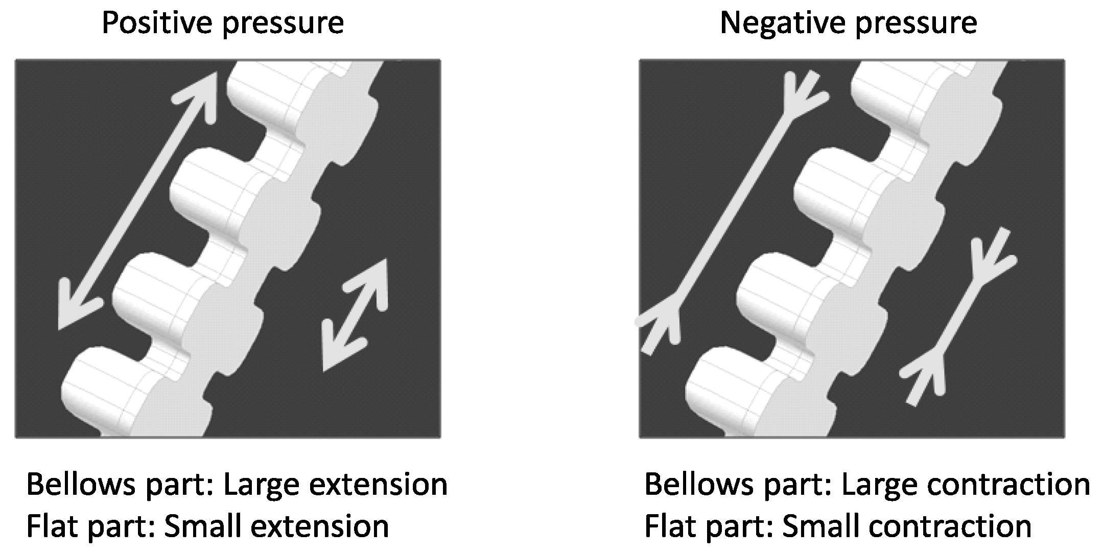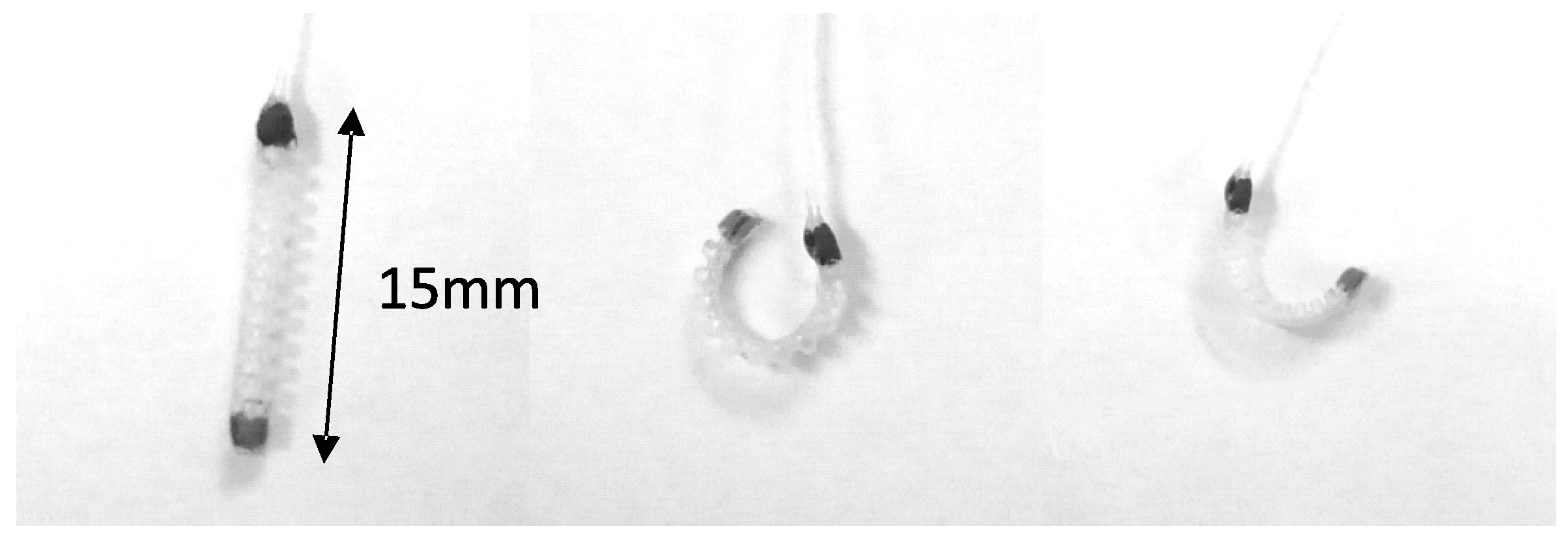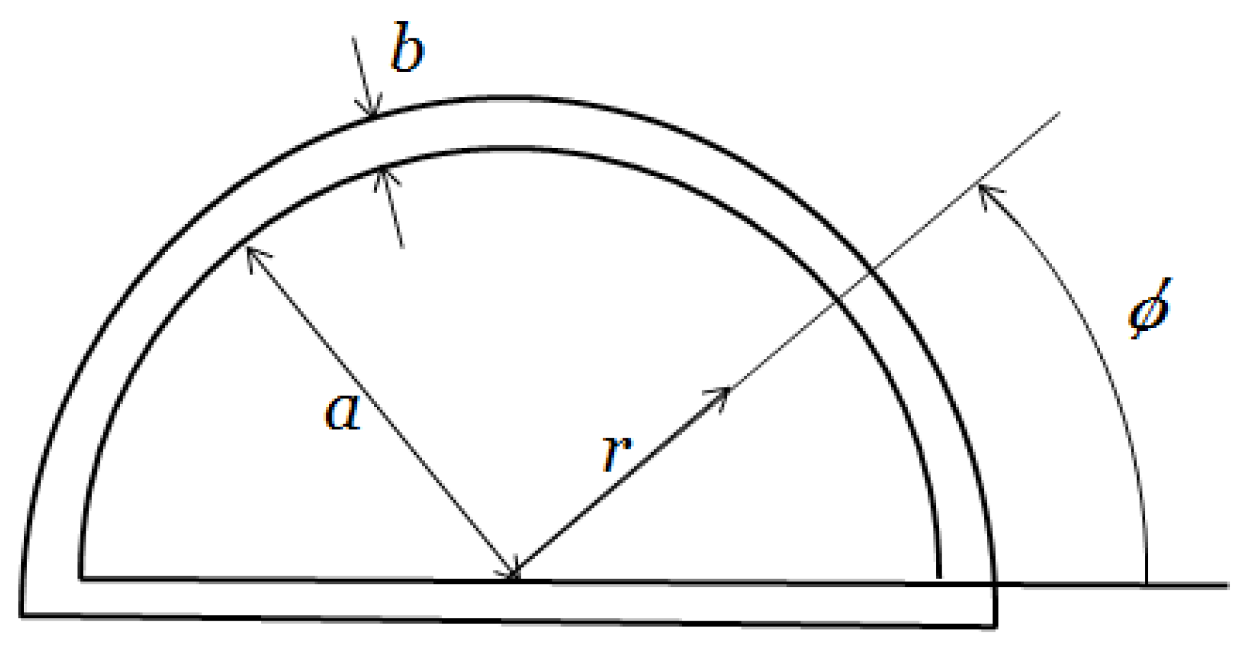Thus, a miniature pneumatic bending rubber actuator [1] was developed to solve these problems as above. A miniature pneumatic bending rubber actuator is one of the soft actuators. It is made of silicone rubber and has a bellows construction on one side. Because of its structure, a miniature pneumatic bending rubber actuator can be made simply, small and inexpensively (a miniature pneumatic bending rubber actuator is often called “a micro-hand” because it will be used in three actuators). On the other hand, this actuator is difficult to model and control due to its nonlinearity. This actuator should be controlled by without sensors, because it is expected to be used for medical fields, especially in operations. Moreover, we have no sensor that can attach itself to this actuator directly because this actuator is too small. Thus, a motion estimation method and nonlinear control system are needed for this actuator.

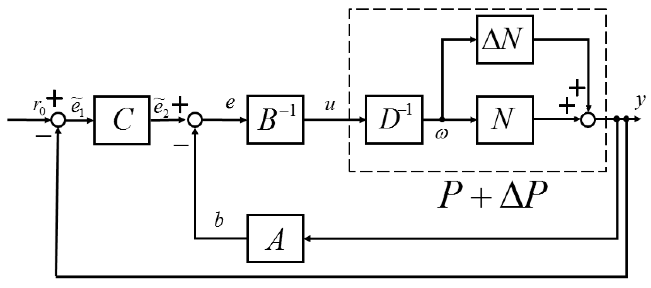
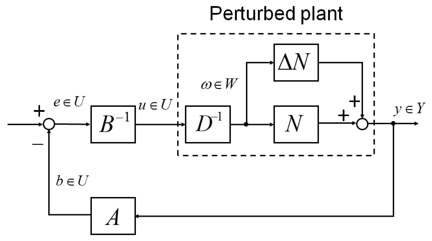
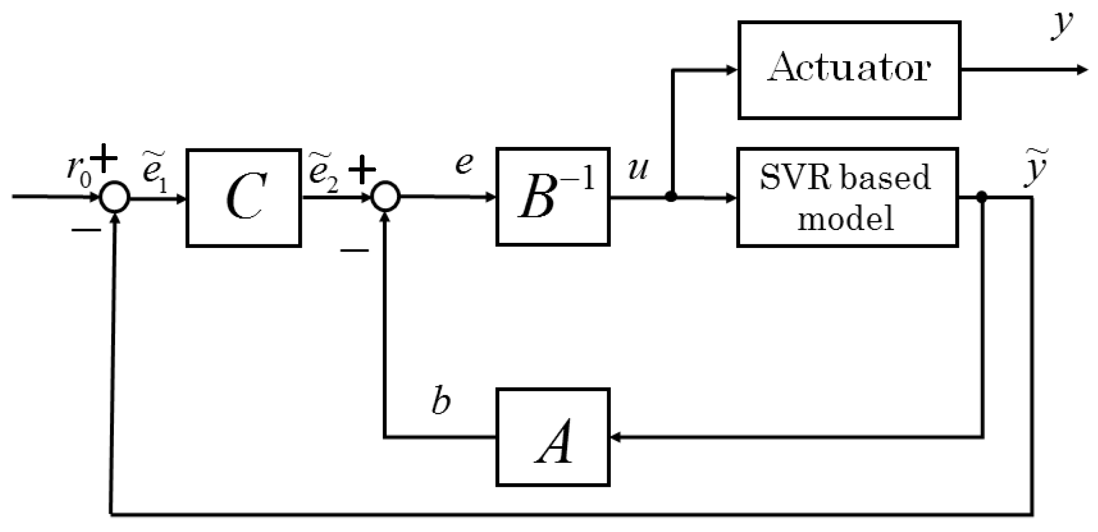
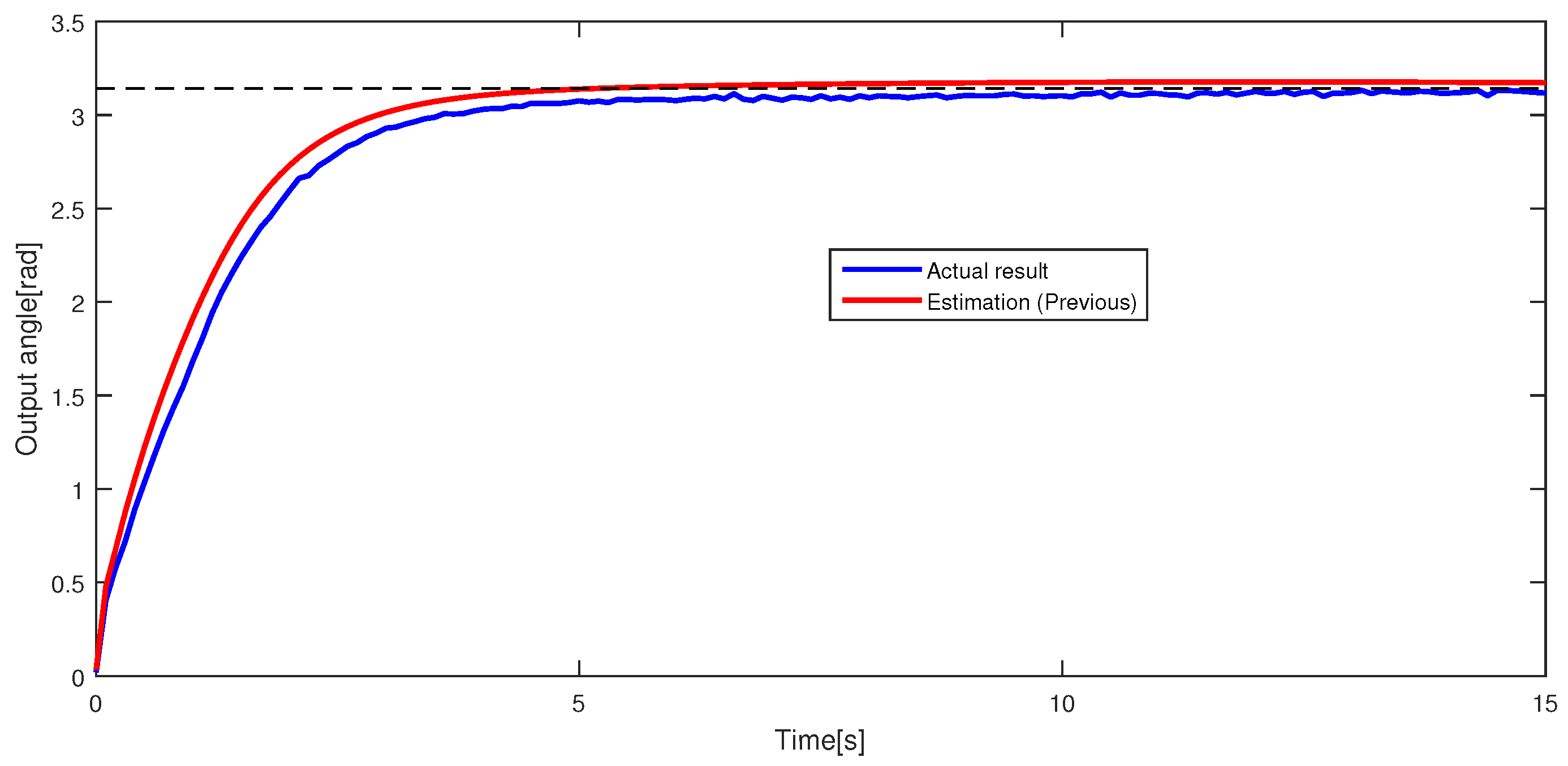
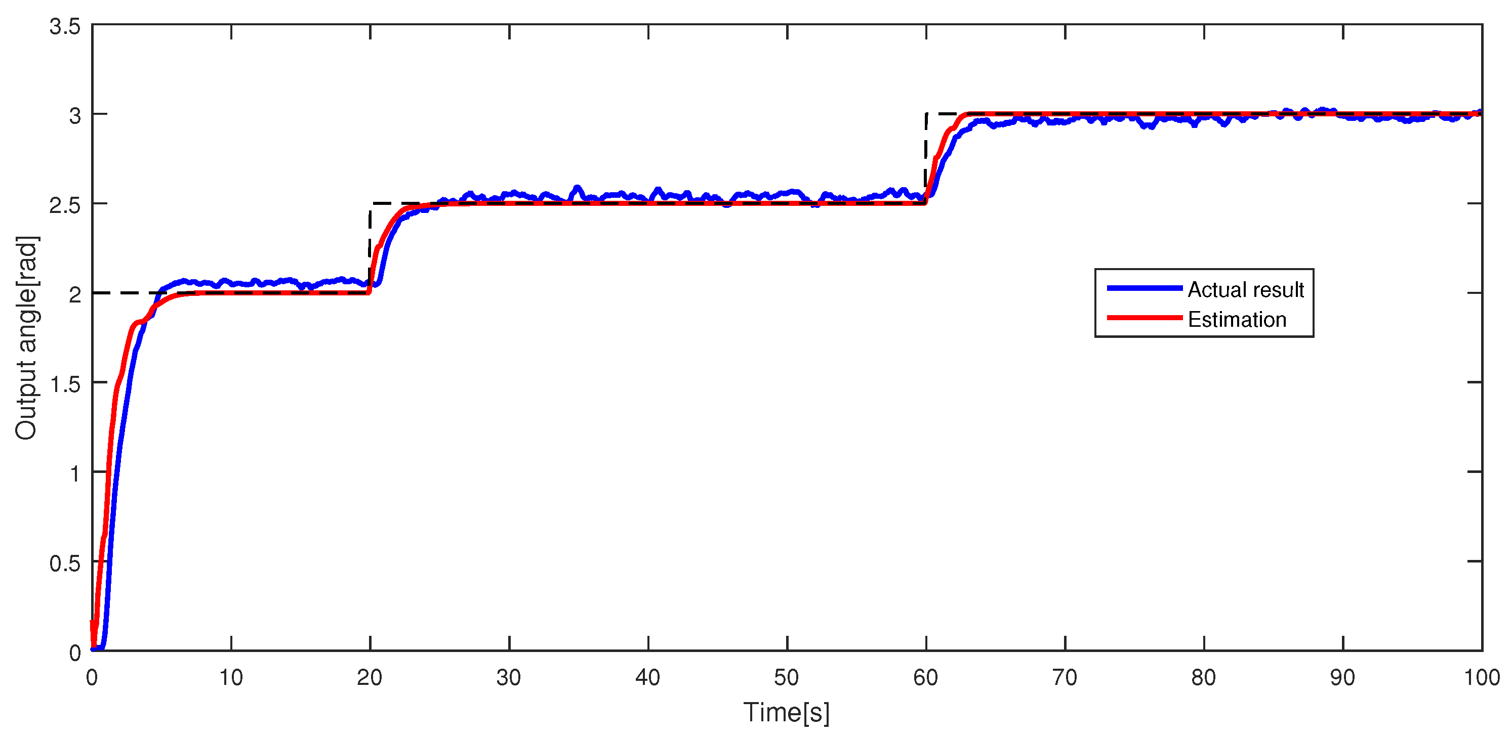
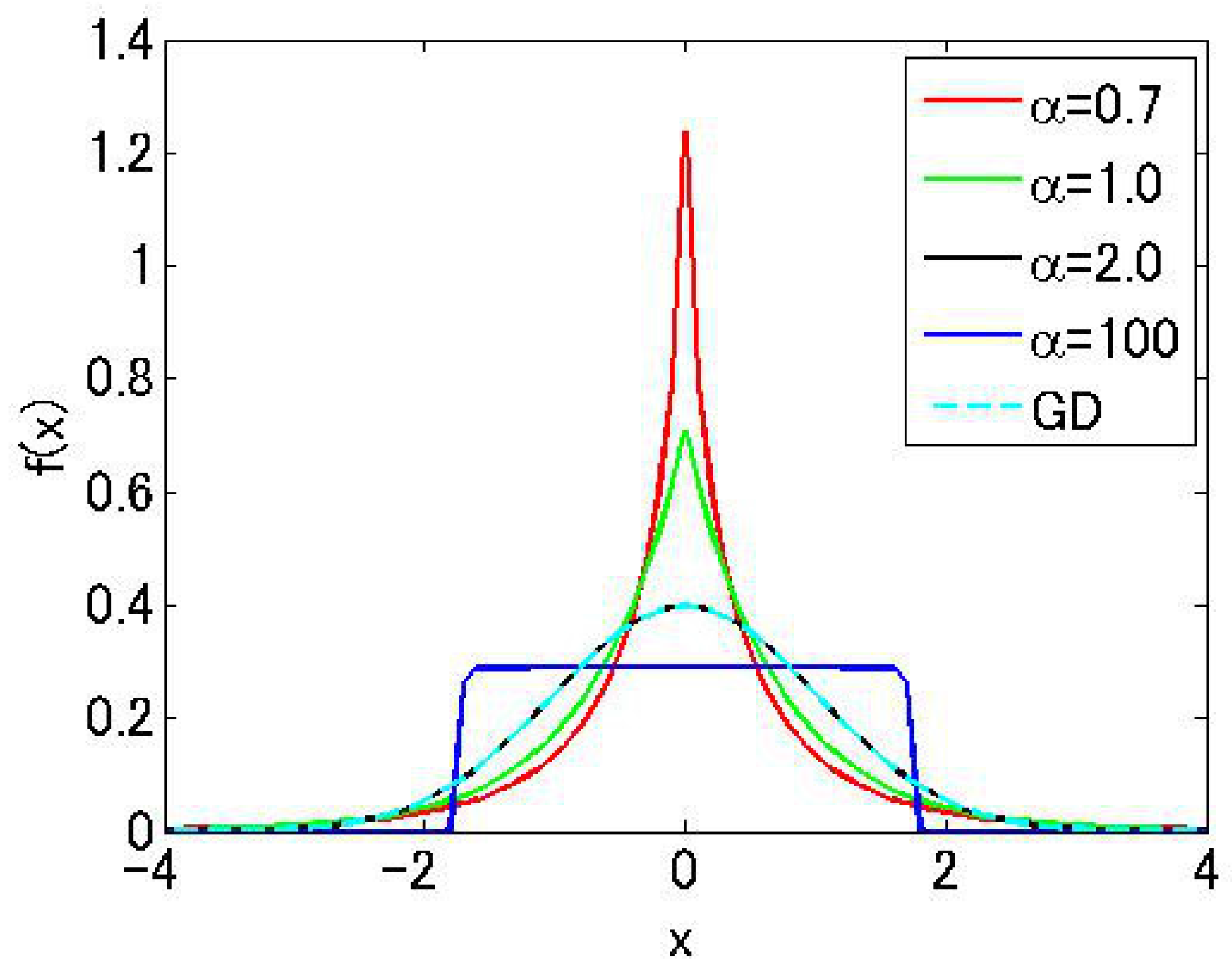
In this paper, support vector regression (SVR) is utilized for output estimation. SVR is a regression machine that is extended from support vector machine (SVM) [2,3,4]. SVR has been utilized by many researchers recently. SVR has some advantages, for example high generalization ability with few training data and valid for a nonlinear model, etc. SVR uses the kernel method. The kernel method makes SVR’s calculation easier. If one function satisfies some properties, it can become a kernel function. Various kernel functions are used for SVR. Especially, the Gaussian kernel, which is applied by the Gaussian distribution (GD), is mainly used for a kernel function in SVR. However, many distributions do not follow GD. The distribution of this actuator is also the same. To solve this problem, SVR with the generalized Gaussian kernel, which is applied from the generalized Gaussian distribution (GGD) [5], for the estimation of the actuator was proposed [6]. The effectiveness of SVR with the generalized Gaussian kernel was verified. Thus, this research utilizes GGD for a kernel function. SVR with the GGD kernel has four parameters. Selecting good parameters is needed to improve the estimation ability of SVR. In this paper, particle swarm optimization (PSO) [7] is utilized for the parameter selecting method. 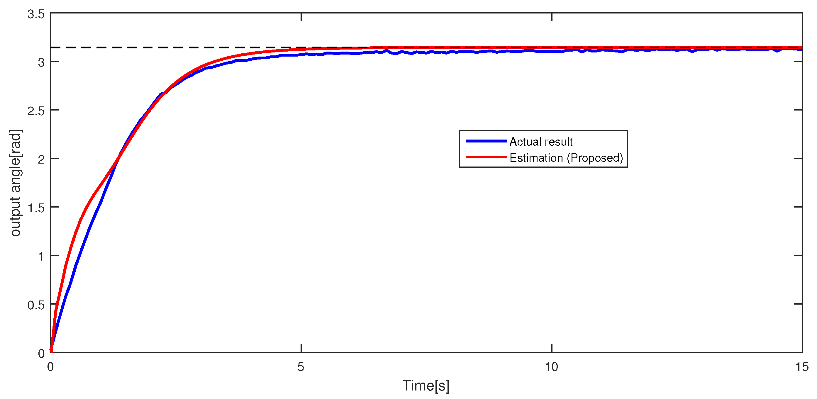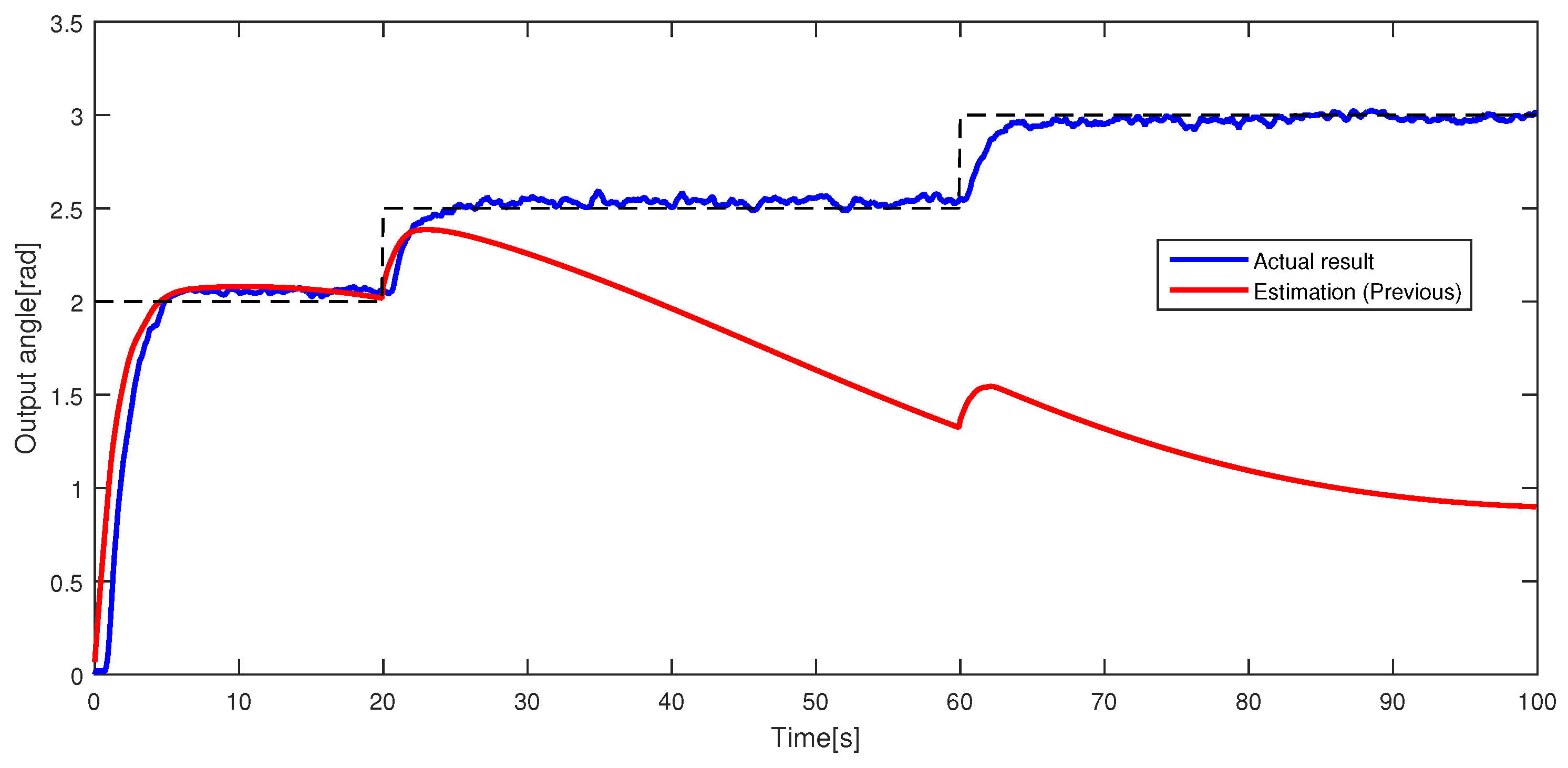In previous research [4], SVR-based estimation and nonlinear control for this actuator are considered. However, the estimation ability can be improved. Thus, this research considers improving estimation ability by the method above. 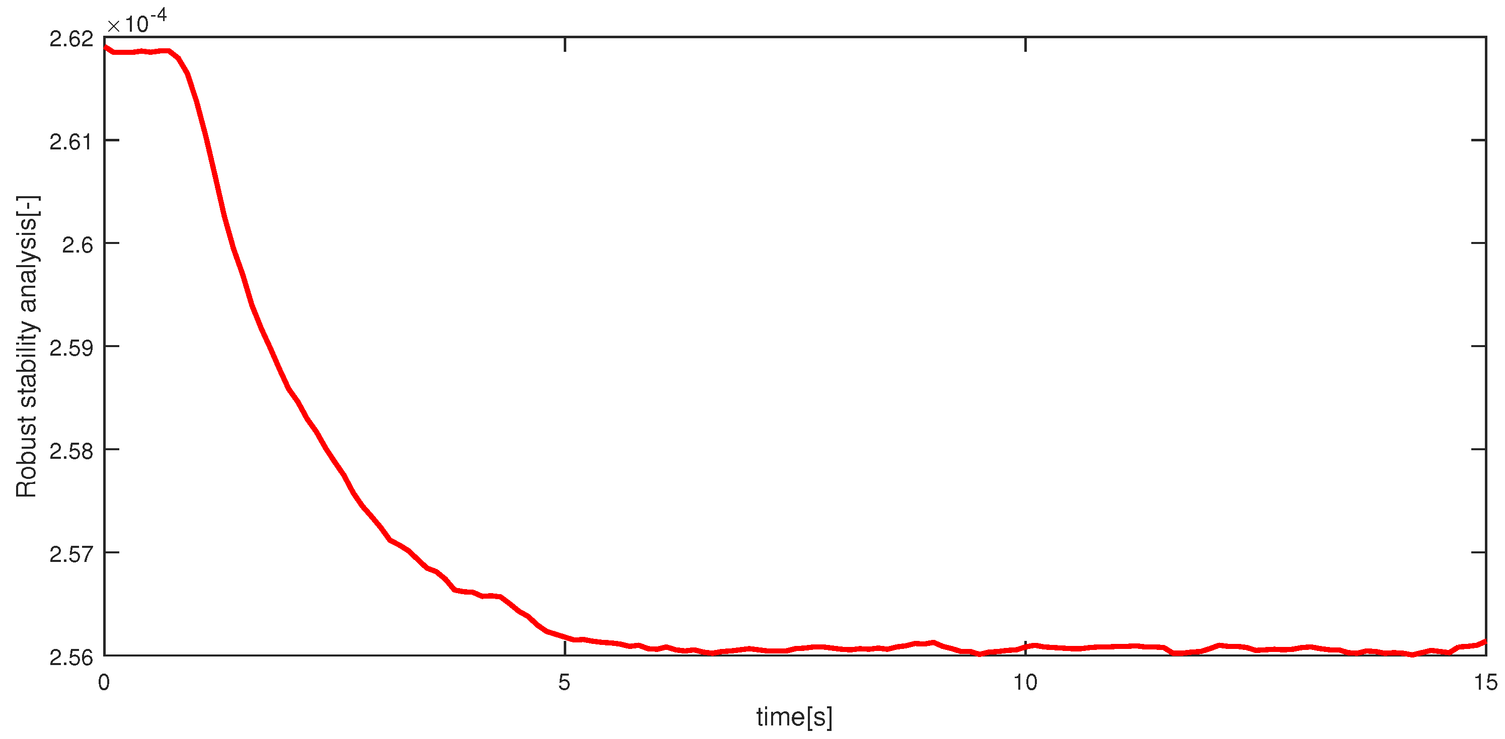To verify the proposed estimation method, an experiment was conducted with a nonlinear control system based on operator theory [8,9,10,11,12].

2. Structure of a Miniature Pneumatic Bending Rubber Actuator

In this section, the structure of the miniature pneumatic bending rubber actuator [1] is explained. The actuator is made of silicone rubber without fiber reinforcement and designed by using the finite element method (FEM). Figure 1 shows the appearance and moving principle of the actuator. The actuator is bent by providing air pressure. The actuator has a semicircular-shaped tube, and one side has a bellows construction. Its bellows part extends and contracts greatly by positive and negative air pressure. Its flat part extends and contracts slightly by positive and negative air pressure. The difference of the extension and contraction between the bellows and the flat part cause its bending motion. Because of this structure, the actuator can bend without using fiber reinforcement. Moreover, the structure of the bellows makes the actuator bend greatly. The actuator can be made small and inexpensive because a micro-hand has only one tube, and the actuator does not use fiber-reinforced rubber.

In case of providing positive air pressure, the bellows part expands greatly and the flat part expands slightly. Therefore, the actuator bends with the state for which the bellows part is outside. On the other hand, in the case of providing negative air pressure, the bellows part shrinks greatly, and the flat part shrinks slightly. Therefore, the actuator bends with the state for which the flat part is outside. For the reasons stated above, the actuator can perform two-way bending with only one tube by providing air pressure. The thickness of silicon rubber and the minimum diameter of the expansion chamber were designed to bend efficiently by using nonlinear finite element analysis. Figure 2 shows the states of movement when air pressure is provided for the actuator.

This can ensure the two-way bending of the actuator according to positive or negative air pressure being provided. The force characteristics were studied in [1]. The measurement range is from 0 to 40 $\mathrm{kPa}$ under positive pressure and from $-16$ to 0 $\mathrm{kPa}$ under negative pressure. The maximum force are $2.2$ $\mathrm{mN}$ at 40 $\mathrm{kPa}$ and $0.6$ $\mathrm{mN}$ at $-16$ $\mathrm{kPa}$.

3. Mathematical Preliminaries

3.1. Support Vector Regression

In this paper, we utilize support vector regression (SVR) [2,3,4]. SVR is an extension of SVM for regression. SVR makes a model from relationship between inputs and outputs. The goal of SVR is to identify a function $f(\mathit{x})$ from the training data. SVR is available for nonlinear functions and has generalization capability. The regression model $f(\mathit{x})$ is shown as

$$\begin{array}{c}\hfill f(\mathit{x})={\mathit{\omega }}^T\varphi (\mathit{x})+b,\end{array}$$

(1)

where $\mathit{x}$ means the input vector, $\mathit{\omega }$ shows the weight vector, b is the offset and $\varphi (\mathit{x})$ is a nonlinear function that maps the input space into a higher dimensional feature space. In the SVM modeling, the slack variables are

$$\begin{array}{cc}\hfill {\xi }_i^{+}& =\left\{\begin{array}{cc}0\hfill & (y_i-f({\mathit{x}}_i)\le ϵ)\hfill \\ y_i-f({\mathit{x}}_i)-ϵ\hfill & (y_i-f({\mathit{x}}_i)>ϵ)\mathrm{and}\hfill \end{array}\right.\hfill \end{array}$$

(2)

$$\begin{array}{cc}\hfill {\xi }_i^{-}& =\left\{\begin{array}{cc}0\hfill & (y_i-f({\mathit{x}}_i)\ge -ϵ)\hfill \\ -ϵ-y_i+f({\mathit{x}}_i)\hfill & (y_i-f({\mathit{x}}_i)<-ϵ),\hfill \end{array}\right.\hfill \end{array}$$

(3)

where ϵ is a configuration parameter and $({\mathit{x}}_i,y_i)$ is the training data. Then, the SVR approach defines an optimization problem as follows.

$$\begin{array}{c}\hfill \underset{\mathit{\omega },b,\xi }{\min }[\frac{1}{2}{\mathit{\omega }}^T\mathit{\omega }+C\sum _{i=1}^n({\xi }_i^{+}+{\xi }_i^{-})]\end{array}$$

(4)

Subject to equality constraints,

$$\begin{array}{c}\hfill \left\{\begin{array}{cc}{y}_i-{\mathit{\omega }}^T\varphi ({\mathit{x}}_i)-b\hfill & \le ϵ+{\xi }_i^{+},i=1,\cdots n\hfill \\ {\mathit{\omega }}^T\varphi ({\mathit{x}}_i)+b-y_i\hfill & \le ϵ+{\xi }_i^{-},i=1,\cdots n\hfill \\ {\xi }_i^{+},{\xi }_i^{-}\hfill & \ge 0,i=1,\cdots n,\hfill \end{array}\right.\end{array}$$

(5)

where C controls the penalty associated with deviations larger than ϵ and n is the number of training data.

Introducing Lagrange multipliers ${\lambda }_i^{+}$, ${\lambda }_i^{-}$, ${\mu }_i^{+}$ and ${\mu }_i^{-}$, Equation (5) can be rewritten as the following optimization problem,

$$\begin{array}{c}{L}_p=\frac{1}{2}{\mathit{\omega }}^T\mathit{\omega }+C_0\sum _{i=1}^n({\xi }_i^{+}+{\xi }_i^{-})-\sum _{i=1}^n{\lambda }_i^{+}\left(ϵ+{\xi }_i^{+}-y_i+{\mathit{\omega }}^T\varphi ({\mathit{x}}_i)+b\right)\hfill \\ \phantom{L_p=\frac{1}{2}{\mathit{\omega }}^T\mathit{\omega }+C_0\sum _{i=1}^n({\xi }_i^{+}+{\xi }_i^{-})-}-\sum _{i=1}^n{\lambda }_i^{-}\left(ϵ+{\xi }_i^{-}+y_i-{\mathit{\omega }}^T\varphi ({\mathit{x}}_i)-b\right)-\sum _{i=1}^n\left({\mu }_i^{+}{\xi }_i^{+}+{\mu }_i^{-}{\xi }_i^{-}\right).\hfill \end{array}$$

(6)

Optimum solutions are the points where the partial differentiation of $L_p$ about $\mathit{\omega },b,{\xi }^{+},{\xi }^{-}$ is zero, so the following equations hold for the optimum solutions.

$$\begin{array}{cc}\hfill \frac{\partial L_p}{\partial \mathit{\omega }}& =\mathit{\omega }-\sum _{i=1}^n({\lambda }_i^{+}-{\lambda }_i^{-})\varphi ({\mathit{x}}_i)=0\hfill \end{array}$$

(7)

$$\begin{array}{cc}\hfill \frac{\partial L_p}{\partial b}& =\sum _{i=1}^n({\lambda }_i^{-}-{\lambda }_i^{+})=0\hfill \end{array}$$

(8)

$$\begin{array}{cc}\hfill \frac{\partial L_p}{\partial {\xi }_i^{+}}& =C_0-{\lambda }_i^{+}-{\mu }_i^{+}=0\hfill \end{array}$$

(9)

$$\begin{array}{cc}\hfill \frac{\partial L_p}{\partial {\xi }_i^{-}}& =C_0-{\lambda }_i^{-}-{\mu }_i^{-}=0\hfill \end{array}$$

(10)

From Equation (7), the vector $\mathit{\omega }$ is shown as

$$\begin{array}{c}\hfill \mathit{\omega }=\sum _{i=1}^n({\lambda }_i^{+}-{\lambda }_i^{-})\varphi ({\mathit{x}}_i).\end{array}$$

(11)

Equation (1) is rewritten as

$$\begin{array}{c}\hfill f(\mathit{x})=\sum _{i=1}^n({\lambda }_i^{+}-{\lambda }_i^{-})\varphi {({\mathit{x}}_i)}^T\varphi (\mathit{x})+b.\end{array}$$

(12)

An optimization problem holds by substituting Equations (7), (9) and (10) for Equation (6).

$${\max }_{{\lambda }_i^{-},{\lambda }_i^{+}}{L}_p={\max }_{{\lambda }_i^{-},{\lambda }_i^{+}}[-\frac{1}{2}{\sum }_{i=1}^n{\sum }_{j=1}^n({\lambda }_i^{+}-{\lambda }_i^{-})({\lambda }_j^{+}-{\lambda }_j^{-})\varphi {({\mathit{x}}_i)}^T\varphi ({\mathit{x}}_j)+{\sum }_{i=1}^n{y}_i\left({\lambda }_i^{+}-{\lambda }_i^{-}\right)-{\sum }_{i=1}^nϵ\left({\lambda }_i^{+}+{\lambda }_i^{-}\right)]$$

(13)

Constraint conditions are shown as follows.

$$\begin{array}{c}\hfill \left\{\begin{array}{c}{\displaystyle \sum _{i=1}^n\left({\lambda }_i^{+}-{\lambda }_i^{-}\right)=0}\hfill \\ 0\le {\lambda }_i^{+},{\lambda }_i^{-}\le C_0\hfill \end{array}\right.\end{array}$$

(14)

A kernel function is shown as follows.

$$\begin{array}{c}\hfill K({\mathit{x}}_i,{\mathit{x}}_j)=\varphi {({\mathit{x}}_i)}^T\varphi ({\mathit{x}}_j)\end{array}$$

(15)

Applying a kernel function, Equation (13) is rewritten as follows.

$$\begin{array}{c}\hfill \underset{{\lambda }_i^{-},{\lambda }_i^{+}}{\max }[-\frac{1}{2}\sum _{i=1}^n\sum _{j=1}^n\left({\lambda }_i^{+}-{\lambda }_i^{-}\right)\left({\lambda }_j^{+}-{\lambda }_j^{-}\right)K\left({\mathit{x}}_i,{\mathit{x}}_j\right)+\sum _{i=1}^n{y}_i\left({\lambda }_i^{+}-{\lambda }_i^{-}\right)-\sum _{i=1}^nϵ\left({\lambda }_i^{+}+{\lambda }_i^{-}\right)]\end{array}$$

(16)

Applying a kernel function, Equation (12) is rewritten as follows.

$$\begin{array}{c}\hfill f(\mathit{x})=\sum _{i=1}^n\left({\lambda }_i^{-}-{\lambda }_i^{+}\right)K({\mathit{x}}_i,\mathit{x})+b\end{array}$$

(17)

The Gaussian kernel is usually used as kernel function and is shown as follows.

$$\begin{array}{c}\hfill K({\mathit{x}}_i,\mathit{x})=\exp \left(-\frac{\parallel {\mathit{x}}_i{-\mathit{x}\parallel }^2}{2{\sigma }^2}\right)\end{array}$$

(18)

3.2. Generalized Gaussian Distribution

The generalized Gaussian distribution (GGD) [5] is used for a kernel function to improve the ability of generalization in this paper. The generalized Gaussian distribution includes all normal and Laplace distributions and all continuous uniform distributions on bounded intervals of the real line. The probability density function (PDF) of GGD with mean μ and shape parameter α is given by

$$f(x;\mu ,\alpha ,\beta )=\left[\frac{\alpha }{2\beta \mathrm{\Gamma }(1/\alpha )}\right]\exp \left\{-{\left[\frac{\parallel x-\mu \parallel }{\beta }\right]}^{\alpha }\right\}\mathrm{and}$$

(19)

$$\beta =\sigma \sqrt{\frac{\mathrm{\Gamma }(1/\alpha )}{\mathrm{\Gamma }(3/\alpha )}},$$

(20)

where Γ defines the Gamma function given by $\mathrm{\Gamma }(z)={\int }_0^{+\infty }{e}^{-t}{t}^{z-1}dt(z>0)$. μ, $\alpha (>0)$ and β denote the mean, shape and scale parameters, respectively. GGD can match many distribution by changing shape parameter α. GGD is applied for the kernel function in this paper.

Figure 3 illustrates the PDFs of generalized Gaussian distribution for various α with $\mu =0$ and $\sigma =1$. Two special cases are the Laplacian distribution for $\alpha =1$ and the Gaussian distribution for $\alpha =2$. For the limited case of α, generalized Gaussian distribution approaches an impulse function and the uniform distribution as $\alpha \to 0$ and $\alpha \to \infty$, respectively.

The generalized Gaussian kernel is given as follows.

$$f({\mathit{x}}_{\mathit{i}},\mathit{x};\alpha ,\beta )=\left[\frac{\alpha }{2\beta \mathrm{\Gamma }(1/\alpha )}\right]\exp \left\{-{\left[\frac{\parallel {\mathit{x}}_{\mathit{i}}-\mathit{x}\parallel }{\beta }\right]}^{\alpha }\right\}$$

(21)

$$\beta =\sigma \sqrt{\frac{\mathrm{\Gamma }(1/\alpha )}{\mathrm{\Gamma }(3/\alpha )}}$$

(22)

3.3. Particle Swarm Optimization

Particle swarm optimization (PSO) [7] is a population-based stochastic approach for solving continuous and discrete optimization problems. The algorithm of PSO is given as follows.

• Initialize the particle’s position and velocity in the swarm randomly, and set ranges of position and velocity.
• Evaluate positions with the evaluation function.
• Update the particle’s and global best solution.
• Update the particle’s velocity and position.

The particle’s velocity and position are updated by the following equations,

$$\begin{array}{cc}\hfill {\mathit{v}}_i(t+1)& =\omega {\mathit{v}}_i(t)+c_1\times ran{d}_1\times [{\mathit{pbest}}_i(t)-{\mathit{p}}_i(t)]+c_2\times ran{d}_2\times [\mathit{gbest}(t)-{\mathit{p}}_i(t)]\hfill \end{array}$$

(23)

$$\begin{array}{cc}\hfill {\mathit{p}}_i(t+1)& ={\mathit{p}}_i(t)+{\mathit{v}}_i(t+1),\hfill \end{array}$$

(24)

where $i=1,$$2,...,$ n; t is the step; $\mathit{p}, \mathit{v}$ are the particle’s position and velocity; $\mathit{pbest}, \mathit{gbest}$ are the particle’s and group’s (swarm’s) best value; ω is the inertial weight coefficient; $c_1,c_2$ are the acceleration constants; $ran{d}_1,ran{d}_2$ are positive random numbers whose range is [0,1].

The inertial weight w controls the effect of the previous velocity to the current velocity. A larger w searches a solution with a wider area, and a smaller w searches a narrower area. To balance the effect of ω, the following equation is used in this paper.

$$\omega ={\omega }_{max}-\frac{t({\omega }_{max}-{\omega }_{min})}{t_{end}}$$

(25)

4. Modeling and Nonlinear Control System

In this section, the modeling and designing of a nonlinear control system [9] for a micro-hand are shown.

4.1. Modeling

Modeling of the actuator [4] is done in this section. It is supposed that the actuator curves in an arc. Bending angle $\theta \in [0,2\pi ]$ is defined in Figure 4. The tip of the actuator in the initial state is regarded as the origin of the coordinates. The horizontal direction is the x-axis, and the vertical direction is the y-axis. The $(x,y)$ is the coordinate of the tip of the actuator at the time of deformation. The parameters in Figure 4 are given in

Table 1. Parameters of the actuator analysis model.

Part of the Actuator	Parameter	Unit
Natural length of the actuator	$L_0$	(m)
Length of the changeless part	$L_1$	(m)
Length of the bellows side	L	(m)
Radius of the approximate circle	R	(m)
Bending angle	θ	(rad)

. The following formulas are derived from Figure 4.

$$\begin{array}{cc}\hfill L& =R\theta \hfill \end{array}$$

(26)

$$\begin{array}{cc}\hfill x& =R-R\cos \theta \hfill \end{array}$$

(27)

$$\begin{array}{cc}\hfill y& =L_0-R\sin \theta \hfill \end{array}$$

(28)

From Equations (27) and (28), R and θ are obtained by

$$\begin{array}{cc}\hfill R& =\frac{x^2+y^2-2L_{0}y+{L_0}^2}{2x}\hfill \end{array}$$

(29)

$$\begin{array}{cc}\hfill \theta & =2{\cos }^{-1}\left(\frac{L_0-y}{\sqrt{x^2+{(L_0-y)}^2}}\right).\hfill \end{array}$$

(30)

A cross-section drawing of the actuator is shown in Figure 5. The cross-section radius of the actuator is a (m). The thickness of the actuator is b (m). The center of the flat side is defined as the origin of polar coordinate system. The radius vector is r (m), and the argument is ϕ (rad). Then, it is supposed that the cross-section shape and the length of the flat side are changeless in order to analyze the theoretical properties of the actuator. The effect by the shape of the bellows part is considered as the uncertainty. The mathematical model is derived from the balance between the moment generated by pneumatic pressure and the one generated by spring force.

The force $f_1$ (N) generated by pneumatic pressure p (Pa) in a small area of the end section of the actuator is shown as:

$$f_1=prd\varphi dr.$$

(31)

Then, the moment of the force generated by pneumatic pressure $M_1$ (N·m) is shown as:

$$\begin{array}{c}\hfill M_1={\int }_0^a{\int }_0^{\pi }{f}_1(r\sin \varphi +b)=\frac{4a^3+3\pi a^{2}b}{6}p.\end{array}$$

(32)

The force $f_2$ (N) generated by the spring in a small area of the bellows side is shown as:

$$f_2=-\frac{E\theta (r_a\sin \varphi +b)}{L_0}b{r}_{a}d\varphi ,$$

(33)

where $r_a(\mathrm{m})$ is the length from the origin of polar coordinate to the center of rubber shown as:

$$r_a=a+\frac{b}{2},$$

(34)

and E (Pa) is the Young modulus. It is supposed that the Young modulus changes according to the extension of rubber equivalently. $E(\mathrm{Pa})$ is shown as

$$E=E_0\frac{L_0}{L_0+\theta (r_a\sin \varphi +b)},$$

(35)

where $E_0$ (Pa) is the initial Young modulus. Then, the moment of the force generated by spring force $M_2$ (N·m) is shown as

$$\begin{array}{cc}\hfill M_2& =-{\int }_0^{\pi }{f}_2(r_a\sin \varphi +b)\hfill \\ & =-r_{a}b{E}_0\theta {\int }_0^{\pi }\frac{{(r_a\sin \varphi +b)}^2}{L_0+\theta (r_a\sin \varphi +b)}d\varphi .\hfill \end{array}$$

(36)

From the balance between the moment generated by pneumatic pressure and the one generated by spring force in the end section of the actuator,

$$M_1+M_2=0.$$

(37)

Then, the relationship between input p and output θ is obtained from Equations (32), (36) and (37),

$$\frac{4a^3+3\pi a^{2}b}{6}p=r_{a}b{E}_0\theta {\int }_0^{\pi }\frac{{(r_a\sin \varphi +b)}^2}{L_0+\theta (r_a\sin \varphi +b)}d\varphi .$$

(38)

Equation (38) is approximated as follows.

$$\theta =-\frac{L_0}{b}\left(1+\frac{2r_a+b\pi }{\gamma p-2r_a-b\pi }\right),$$

(39)

where

$$\gamma =\frac{4a^3+3\pi a^{2}b}{6r_{a}b{E}_0}.$$

(40)

4.2. Design for the Operator-Based Robust Nonlinear Control System

The robust nonlinear control system based on robust right coprime factorization for the actuator is designed in this section [8,9,10,11,12]. Consider the nonlinear feedback system in Figure 6.

Nominal plant P is shown as

$$P(u)(t)=-\frac{L_0}{b}\left(1+\frac{2r_a+b\pi }{\gamma u(t)-2r_a-b\pi }\right),$$

(41)

where input $u=p$, output $y=\theta$ and γ is Equation (40). The plant P is factorized into N and $D^{-1}$:

$$\begin{array}{cc}\hfill N(\omega )(t)& =-\frac{L_0}{b}\left(1+\frac{2(2r_a+b\pi )}{\omega (t)-2(2r_a+b\pi )}\right)\mathrm{and}\hfill \end{array}$$

(42)

$$\begin{array}{cc}\hfill D^{-1}(u)(t)& =2\gamma u(t),\hfill \end{array}$$

(43)

where N is stable and D is stable and invertible. According to the Bezout identity:

$$\begin{array}{c}\hfill AN+BD=M(\omega )(t),\end{array}$$

(44)

where M is the unimodular matrix. We have

$$\begin{array}{cc}\hfill A(y)(t)& =(1-K)\left(-\frac{2L_0(2r_a+b\pi )}{by(t)+L_0}+2(2r_a+b\pi )\right)\mathrm{and}\hfill \end{array}$$

(45)

$$\begin{array}{cc}\hfill B(u)(t)& =2K\gamma u(t),\hfill \end{array}$$

(46)

where K is the designed controller parameter, A is stable and B is stable and invertible.

The actual plant has the uncertainty derived from the effect by the shape of the bellows and approximation in modeling. The plant with the uncertainty $P+\Delta P$ is shown as

$$(P+\Delta P)(u)(t)=-(1+\Delta )\frac{L_0}{b}\left(1+\frac{2r_a+b\pi }{\gamma u(t)-2r_a-b\pi }\right).$$

(47)

The right factorization of the nonlinear plant is shown as follows.

$$P+\Delta P=(N+\Delta N)D^{-1}$$

(48)

Then, $P+\Delta P$ is factorized as follows.

$$\begin{array}{cc}\hfill (N+\Delta N)(\omega )(t)& =-(1+\Delta )\frac{L_0}{b}\left(1+\frac{2(2r_a+b\pi )}{\omega (t)-2(2r_a+b\pi )}\right)\hfill \end{array}$$

(49)

$$\begin{array}{cc}\hfill D^{-1}(u)(t)& =2\gamma u(t)\hfill \end{array}$$

(50)

When Equation (44) and

$$\begin{array}{c}\hfill \parallel (A(N+\Delta N)-AN)I^{-1}{\parallel }_{Lip}<1\end{array}$$

(51)

are satisfied, the robust stability of the plant with uncertainty $P+\Delta P$ can be guaranteed.

4.3. Tracking Actuator’s Output for the Target Value

The feedback control system is designed in order to track output y to reference input $r_0$. A nonlinear feedback control system with the tracking controller is shown in Figure 7.

Tracking controller C is defined as follows.

$$\begin{array}{c}\hfill C({\tilde{e}}_1)(t)=k_I{\int }_0^t{\tilde{e}}_1(\tau )d\tau +k_P{\tilde{e}}_1(t),\end{array}$$

(52)

where $k_I$ and $k_P$ are the designed parameters.

5. Proposed Method

In this section, the proposed method is introduced. A pneumatic bending rubber actuator is difficult to control and make a model of due to its complicated construction. Moreover, there are no sensors to measure the output of the actuator. The research objective is to estimate the motion of the actuator and apply it for its control. SVM-based regression (SVR) is employed to estimate the motion of the actuator. SVR has high generalization ability with few training data and valid for nonlinear systems. SVR is one of the kernel methods. Thus, SVR uses a kernel function. This kernel function influences the estimation accuracy of SVR. Various kernel functions were developed so far. The most used kernel function is the Gaussian kernel in Equation (18). However, most distributions do not follow the Gaussian distribution. Therefore, the generalized Gaussian kernel (Equation (21)) is employed in this paper. SVR with the generalized Gaussian kernel has four parameters, which should be optimized. PSO is employed as a parameter optimizing method in this paper. PSO has the advantage that calculation cost of PSO is not increased with the increasing of the number of optimized parameters. Four parameters of SVR are optimized by PSO in this paper. The control system [9] is designed to verify the effectiveness of the proposed method. The control system with SVR estimation is shown as Figure 8; where y and $\tilde{y}$ are actuator and estimation output, respectively, and $A,B$ and C are in Equations (45), (46) and (52), respectively.

The proposed method, a motion estimation method for a control system of a pneumatic bending rubber actuator using the PSO-SVR method with the generalized Gaussian kernel, is verified by using this system. In the proposed method, four parameters (C, ε, σ, α) should be optimized, where C, ε are the parameters of SVR and σ, α are the parameters of the generalized Gaussian kernel function. In order to optimize these parameters, grid search is often used. However, grid search needs a huge amount of calculating. Thus, PSO is utilized in this paper. If the optimized parameters are increased, the calculation cost is not increased.

The following is the summary of above.

• Input training data for SVR with the generalized Gaussian kernel.
• Do many tests and evaluations with various parameters.
• Decide the best parameters.
• Estimate the actuator’s output by SVR with the optimized parameters.

6. Experiment

6.1. Experimental System

The experimental system is explained in this section. Figure 9 shows the experimental system and actuator. Figure 10 shows the flowchart of the experimental system.

The pump and the electronic vacuum regulator and the vacuum regulator are not used because the actuator’s moving by only positive pressure is considered in this paper. The following explains how to move the actuator.

• Compressed air is made by the air compressor.
• Air pressure is regulated by the regulator to prevent the actuator from breaking.
• Controlled air pressure is made to control the actuator by the electro-pneumatic regulator.
• Air pressure is provided for the actuator, and it moves.

The electro-pneumatic regulator is the equipment that converts electric signals into air pressure. In this paper, ITV0010-0CS (SMC, Tokyo, Japan) is used as the electro-pneumatic regulator. It can convert 4 to 20 $\mathrm{mA}$ into 1 to 100 $\mathrm{kPa}$. The electrical signal is generated by the PC. In this paper, a camera is used to measure position of the actuator. The camera measures the position of the actuator; however, the measurement value from the camera is not used as the feedback signal in order to perform sensorless control. The measurement value is used only to record.

6.2. Experimental Result

The experimental result of the proposed method is shown. First, the selected parameters by PSO are shown in

Table 2. Selected parameters.

Parameter	Value
Cost parameter	$C=100$
Error accuracy parameter	$\epsilon =0.001$
Variance	$\sigma =39.5712$
Shape parameter	$\alpha =2.027$

.

Table 3. Experimental parameters.

Paramter	Value
Natural length of the actuator	$L_0=1.35\times {10}^{-2}$ m
Radius of the actuator	$a=1.0\times {10}^{-3}$ m
Thickness of the actuator	$b=0.15\times {10}^{-3}$ m
Rubber radius	$r_a=1.075\times {10}^{-3}$ m
Initial Young modulus	$E_0=1.43\times {10}^6$ Pa
Control parameter	$K=0.95$
Integral parameter	$k_I=8.0\times {10}^{-6}$
Proportional parameter	$k_P=5.0\times {10}^{-6}$

shows the experimental parameters.

The output results of the proposed and previous method [4] are shown in Figure 11 and Figure 12, respectively. Plant input and robust stability analysis are shown in Figure 13 and Figure 14, respectively. In this experiment, the desired value is $3.14$ $\mathrm{rad}$. The comparison between the proposed and previous methods is shown in

Table 4. The comparison of some values.

	Proposed Method	Previous Method
Number of dataset	1080	5472
Computing time	$5.2$ s	$13.4$ s
Fit ratio	$86.8\%$	$84.8\%$

.

“Number of dataset” means the number of the training dataset used in SVR. SVR estimates the actuator’s output value based on this dataset. “Computing time” means the sum of SVR training time and feedback time. Shorter computing time is better, if the “fit ratios” have the same value. The following equation is used as the evaluation function called the “fit ratio”:

$$\mathrm{Fitness}=\left(1-\frac{\sqrt{{\displaystyle \sum _{k=1}^N{[\tilde{y}(k)-y(k)]}^2}}}{\sqrt{{\displaystyle \sum _{k=1}^N{[y(k)-\overline{y}]}^2}}}\right)\times 100(\%),$$

(53)

where $y(k)$, $\tilde{y}(k)$ and $\overline{y}(k)$ are “actual output or desired value”, “estimation or simulation output” and the average of “actual output or desired value”, respectively. “Fitness” is the ratio of fitting for the actual result. The output result could track the desired value of $3.14$. The proposed method could estimate the actuator’s output more accurately than the previous one. Moreover, the number of the dataset and the computing time of the proposed method were fewer than the previous one. Therefore, the estimation ability of the proposed method was verified. If the system satisfied Equation (51), the system can be said to have robust stability. In Figure 14, $\parallel (A(N+\Delta N)-AN)I^{-1}{\parallel }_{Lip}<1$ is satisfied. Thus, the system is a robust stability system.

Other results are shown as follows. The output and estimation results of the proposed and previous method are shown in Figure 15 and Figure 16, respectively. Plant input and robust stability analysis are shown in Figure 17 and Figure 18, respectively. The comparison between the proposed and previous methods is shown in

Table 5. The comparison of some values.

	Proposed Method	Previous Method
Number of dataset	1437	5414
Computing time	$23.5$ s	$62.8$ s
Fit ratio	$83.5\%$	$-157\%$

. The desired value $r_0$ is as follows.

$$\begin{array}{c}\hfill r_0=\left\{\begin{array}{cc}2\hfill & (0\le t\le 20)\hfill \\ 2.5\hfill & (20<t\le 60)\hfill \\ 3\hfill & (60<t\le 100)\hfill \end{array}\right.\end{array}$$

(54)

The meanings of the “number of dataset”, “computing time” and “fit ratio” are the same as Table 4. The plant output tracked the desired value, so the effectiveness of the control system is verified. In Figure 16, the previous method cannot estimate the plant output accurately. In the previous method, SVR-based estimation depends on experimental time. Thus, estimation ability changes according to experimental time. On the other hand, the proposed method can estimate the plant output accurately in Figure 15. This is because the proposed SVR-based method is not related to time, but position and former position. Therefore, the estimation ability does not depend on the experimental time. Moreover, the generalized Gaussian kernel and the PSO-based parameter optimization are used in the proposed method. Therefore, the proposed estimation method can estimate the plant output accurately. The effectiveness of the estimation method has been verified. Figure 18 shows that the robust stability of the system is verified.

7. Conclusions

In this paper, a motion estimation method for a control system of a pneumatic bending rubber actuator using the PSO-SVR method with the generalized Gaussian kernel was proposed. The estimation ability of SVR was improved by using the generalized Gaussian kernel, selecting the parameters by PSO and considering the dataset of SVR. In conclusion, the effectiveness of the proposed method was proven by the experimental result.