
Transpermeance Amplifier Applied to Magnetic Bearings


1
School of Science and Technology, Federal University of Rio Grande do Norte, Natal-RN 59000-000, Brazil
2
Department of Integrated Science and Technology, James Madison University, Harrisonburg, VA 22807-1003, USA
3
Department of Mechanical and Aerospace Engineering, University of Virginia, Charlottesville, VA 22904-4246, USA
*
Author to whom correspondence should be addressed.
Actuators 2017, 6(1), 9; https://doi.org/10.3390/act6010009
Submission received: 30 November 2016
/
Revised: 24 January 2017
/
Accepted: 7 February 2017
/
Published: 15 February 2017
(This article belongs to the Special Issue Active Magnetic Bearing Actuators)
Abstract
:The most conventional approach of controlling magnetic forces in active magnetic bearings (AMBs) is through current feedback amplifiers: transconductance. This enables the operation of the AMB to be understood in terms of a relatively simple current-based model as has been widely reported on in the literature. The alternative notion of using transpermeance amplifiers, which approximate the feedback of gap flux rather than current, has been in commercial use in some form for at least thirty years, however is only recently seeing more widespread acceptance as a commercial standard. This study explores how such alternative amplifiers should be modeled and then examines the differences in behavior between AMBs equipped with transconductance and transpermeance amplifiers. The focus of this study is on two aspects. The first is the influence of rotor displacement on AMB force, commonly modeled as a constant negative equivalent mechanical stiffness, and it is shown that either scheme actually leads to a finite bandwidth effect, but that this bandwidth is much lower when transpermeance is employed. The second aspect is the influence of eddy currents. Using a very simple model of eddy currents (a secondary short-circuited coil), it is demonstrated that transpermeance amplifiers can recover significant actuator bandwidth compared with transconductance, but at the cost of needing increased peak current headroom.
Keywords:
transpermeance; flux feedback; flux estimation; AMB bandwidth; actuators; amplifiers; eddy current1. Introduction
The use of active magnetic bearings (AMBs) in industrial machinery has seen a significant increase over the past decade due their high speed capabilities and lack of a need for an external lubrication system, resulting in significant improvements in system-level power density, as well as a notable reduction in the equipment package footprint. An efficient AMB system presents a consonant operation between the controller and the mechanical system design. This system must include an effective power amplifier, which is responsible for supplying the actuator with proper levels of voltage and current in order to produce the desired output force over the entire operating frequency range.
Conventional AMB amplifiers, as discussed in the literature, are based on current feedback. This amplifier architecture, also known as transconductance, is then combined with a simple linearized model of the magnet () in order to control the force on the rotor and achieve a stable closed loop system [1,2,3] (This paper uses many mathematical symbols, some conventional to the AMB literature and some selected for the purposes of this paper. For the convenience of the the reader, these symbols and their definitions are collectively presented in Table 1). However, such a model neglects the influence of amplifier dynamics on the term and provides no means to include the effects of magnetic nonlinearity, hysteresis and eddy current effects.
According to Aenis and Nordmann [1], the most accurate method of determining magnetic bearing force is via a flux density measurement. The conclusion in [1] is based on a comparison of different force measurement techniques applied to a radial magnetic bearing system with actuator forces covering a large operating range. Keith [4] analyzes the relationship between actuator flux and generated force and demonstrates that the flux-force relation is invariant to magnetic saturation, which suggests an opportunity for significantly improved bearing performance characteristics under transient and periodic excursions into the saturation region.
Groom [5] proposed a magnetic bearing control approach using flux feedback to produce a linear relationship between the commanded force and the actual output force over a large gap range. A permanent magnet flux bias approach was used, and the results demonstrate excellent agreement between the theoretical predictions and the experimental results achieved via implementing flux feedback on an actual laboratory test rig.
The flux feedback methods mentioned in the references cited above were implemented by means of some sort of flux sensor. Direct flux sensors have numerous drawbacks, including low sensitivity, high cost, space constraints and mechanical fragility. This commends an alternative solution: flux estimation [3,4,6]. These works all describe efficient flux estimation amplifier architectures based on readily available measurements: actuator coil current and voltage. This alternative to the traditional transconductance amplifier is termed a transpermeance amplifier because it produces an output flux proportional to the input reference voltage, analogous to the proportional reference voltage to current output relationship of a transconductance amplifier.
One of the drawbacks of a transconductance amplifier is its degraded behavior in the presence of non-linearities, such as eddy currents. The accurate modeling of eddy current effects is a complex task, which involves many variables. For example, an eddy current model of non-laminated electromagnetic actuators is developed by Zhu et al. [7,8,9]. The work in [7] develops analytic models, which are shown to accurately predict the dynamic behavior of non-laminated axisymmetric electromagnetic actuators, including eddy current effects, and [8] follows a similar formulation for non-laminated C-core electromagnetic actuators. The work in [9] develops equations for both current-mode and voltage-mode operation of electromagnetic actuators, including the effect of time varying rotor position, as well as eddy current effects on the actuator force production. The resulting analytic model is shown to accurately predict the impact of eddy currents on the dynamic behavior of non-laminated magnetic actuators. Whitlow et al. [10] extends the work of [7,8] to the prediction of the dynamic behavior of segmented electromagnetic thrust bearing actuator geometries.
In [11], Zhou and Li present the modeling and identification of a solid C-core active magnetic bearing including eddy currents. The goal is to determine the effect of eddy currents on the system dynamics under both current and voltage drive modes (transconductance and transpermeance, respectively). The results indicate that a voltage-mode drive can effectively reduce the eddy current effects compared with a current-mode drive.
Although accurate models of electromagnetic actuators including eddy current effects have been developed for many practical problems, such as control design, these models can be too complicated and cumbersome to implement effectively. Therefore, simpler models, which capture the primary effects of eddy currents on actuator performance, can also be very useful. The dynamics of non-laminated C-core magnetic actuators were first studied by Zmood et al. [12], resulting in a simple first-order analytic model. Feeley and Ahlstrom [13] develop a relatively simple model, which is convenient to use for control system design of magnetic bearings that experience significant eddy current levels.
The dynamic performance advantage of flux feedback over current feedback has been clearly shown in the literature. In addition, detailed models that accurately predict the dynamic behavior of electromagnetic actuators including eddy current effects have been developed. Additionally, some work has been done that involves current-mode (transconductance) and voltage-mode (transpermeance) amplifier-controlled magnetic bearing system behavior in the presence of eddy currents. However, the systematic, detailed study and performance comparison of transconductance versus transpermeance amplifiers under varying eddy current level remains an open area of investigation.
This paper investigates the performance differences between AMBs equipped with transpermeance amplifiers and those using a more conventional transconductance amplifier architecture. The focus of this paper is on performance impacts related to eddy current effects. An important consideration that has been taken is the development of a generalized model of the amplifier, which through the use of a weighting function can be used to represent either a transconductance or a transpermeance amplifier. A detailed electromagnetic actuator model including a simplified eddy current model is developed based on first principles. The resulting closed loop amplifier-actuator model connects the reference voltage and displacement (inputs) to flux, estimated flux, actuator voltage and current (outputs). Through the use of non-dimensionalization, a parametric study of the ratio of magnetic to estimation time constants and of eddy current level is performed in order to better understand the performance impact of these two parameters, as well as the mechanisms that the two different architectures use to achieve the varying performance levels. Finally, observations and conclusions related to the performance differences seen between the two amplifier types are drawn.
2. Generalized Amplifier Model
A transpermeance amplifier model is based on flux feedback instead of the more traditional current feedback used in a transconductance amplifier [2]. In order to implement a flux feedback amplifier, it is necessary to measure the flux. However, direct flux sensors have many drawbacks, including low sensitivity, high cost, space constraints and mechanical fragility, which encourages the alternative use of flux estimation [6]. The flux may be estimated either by integrating the coil voltage according to Faraday’s law or from the coil current according to Ampere’s law. The former is effective at high frequencies, but not at low frequencies, whereas the latter is effective at low frequencies, but not at high. Thus, a solution to estimating flux is to combine the two approaches as:
in which Faraday’s law is used to estimate and Ampere’s law is used to estimate :
The weighting function achieves the tradeoff between the use of voltage and current in the flux estimate. If , the model represents a pure transconductance amplifier, and if , the amplifier is pure transpermeance. Due to the low frequency errors associated with , it is not practical to implement pure transpermeance. Therefore, practical transpermeance implementation implies the use of frequency-shaped weighting functions , the details of which will be discussed further in Section 3.2.
Once flux is estimated, the remainder of the amplifier model assumes that the coil voltage is obtained from a combination of the amplifier reference signal, u, and the estimated flux, :
The design of and is directed toward achieving some specific relationship between u and : typically, a bandwidth on the order of 1 kHz, a damping ratio slightly lower than 1.0 and a static gain that maps volts to in which is the saturation flux level of the actuator.
Implicit in this model is the assumption that the power gain stage of the amplifier represents a perfect voltage to voltage converter. The reasoning behind this modeling decision was based on the fact that most commercially available power amplifiers operate with PWM frequencies ranging from 20 kHz–100 kHz, while the actuator bandwidth is typically on the order of 1 kHz. This frequency separation means that while not perfect, this model approximation should be quite good for the purposes of this study.
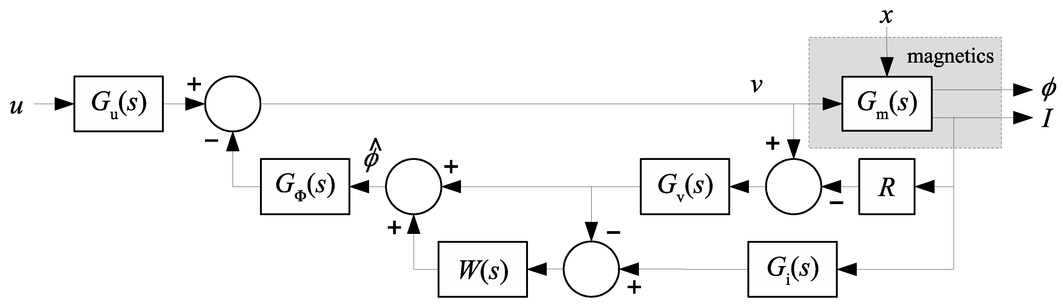
The resulting generalized architecture is illustrated in Figure 1 in which represents the actual response of the physical electromagnet to changes in both the gap length due to rotor motion, x, and to the coil voltage, v. It is important to note that, if the effect of x is removed and the model disregards nonlinearity, hysteresis and eddy currents, then has no effect on the behavior of the system.
3. System Model
The individual subsystem models that make up the amplifier-actuator system are first obtained separately, and then, they are combined together to form the overall system model.
3.1. Actuator Model
In the general AMB literature, the standard simplified model of the actuator (amplifier plus electromagnet) describes the relationship between the reference voltage input and current output: typically, a first- or second-order finite bandwidth model. This current then drives a linearized model of the magnet: . However, a more complete model of the actuator dynamics can be constructed if the internal dynamics that explicitly account for the actual coil voltage and journal displacement is first developed. Such a model uses the reference voltage and journal position as its input signals and produces both current and flux as outputs, as illustrated in Figure 1.
Assume the usual differential arrangement of magnets in the AMB so that opposing pairs of magnets are coordinated in a bias linearization scheme [14]. The resulting flux is proportional to the product of the bias flux and the symmetrically-perturbed control flux. In this manner, the force is linear in the control flux, and the flux output of the actuator model is proportional to force.
Such a model can readily consider magnetic saturation, although that is not the focus of the present work. It can also consider eddy current production and the effect of eddy currents on actuator performance. The eddy current modeling is not easy to achieve with high fidelity and generally leads to either very high order models or to fractional order models. This is a consequence of the way in which eddy currents distribute throughout the volume of the conductive and magnetically-permeable material of the electromagnets, often referred to as the “skin effect”. Zhu et al. [9] provide a thorough discussion of higher fidelity eddy current models.
In the present work, eddy currents have been modeled in a very simple manner meant primarily to illustrate the nature of the effect and its interaction with the two power amplifier schemes considered here. In this model, one extra short-circuited winding is added around the core in order to represent the effect of eddy currents, as shown in Figure 2. The variables N, R, I and V are the number of turns, resistance, current and voltage of the actuator winding and , , and are the same variables for the eddy current winding. Thus, any current induced in this shorted turn is the eddy current, and it represents a model in which the eddy currents are uniformly distributed in a thin layer near the surface of the magnet iron. Many, but not all, features of eddy current production are captured by this simplified model.
Heuristically, the notion behind this simplified model is to show that transpermeance amplifiers eliminate the influence of eddy currents on the bandwidth of the actuator although at some cost in terms of increased voltage and current requirements at high frequencies. Of course, showing that transpermeance amplifiers accomplish this for a specific (and admittedly naive) eddy current model is only of value if the result can be extended to higher fidelity models. The chief drawback to the argument relates to the assumptions of flux uniformity in the gap. That is, the simplified model does not consider the “skin effect”, which means that the magnetic field gets compressed into the perimeter of the magnetic structure with the consequence that the relationship between force and the square of total flux is different at high frequencies (where the skin effect acts) than at low frequencies. This issue is largely mitigated in well-laminated structures where the skin effect leads to very local field non-uniformity, but no large-scale skin effect, and of course, these are the very actuators where eddy current effects are least worrisome. In solid actuators like thrust bearings, the skin effect is much more significant [9], and it is here that the assumptions of the present model will most break down.
The eddy current effects are calculated by assuming that no leakage or fringing occurs in the air gap, the material permeability is finite, but constant and the flux density across any given cross-section is uniformly distributed. The relationship between voltage, flux variation and current at the actuator winding is obtained from the combination of Faraday’s and Ohm’s laws for the two coil loops:
Ampère’s loop law in discrete form then states:
As a matter of notational convenience, let in which is the nominal air gap plus iron path reluctance, x is the position of the rotor relative to magnetic center and α is the sensitivity of the gap to rotor displacement. This sensitivity α would typically be about 1.0, but would be less with a circular rotor and poles on either side of the centerline. Equation (5) gives a simple dynamic relationship between the eddy currents and the flux, and this may be used in Equation (6) to solve for the coil current in terms of the flux and gap:
Further, define a non-dimensional eddy current parameter λ as:
where a completely non-conductive actuator would have and an actuator with a superconducting volume would approximate the limit as . Substitute Equations (7) and (8) into Equation (4), and solve for :
Expanding Equation (9) about and , where and , noting that and assuming that (a linearization assumption) produce:
Define the mean voltage, , as:
and define the perturbation voltage v as:
so that
Now, define the magnetic system time constant as:
to obtain:
Define the mean coil current:
and the perturbation current:
to obtain:
In summary, the state-space system model for the flux system with the simplified eddy current model driven by voltage and rotor position is the combination of Equations (15) and (19):
If such a device is measured using conventional electrical testing methods, the transfer function from voltage to current would be measured with . Therefore, setting in Equation (20) and taking the Laplace transform results in:
Solving for i in terms of v produces:
This transfer function has a pole at and a transmission zero at . The transmission zero is always larger in magnitude than the pole as long as , as it must be in order to make physical sense. In the limit, as λ goes to zero, the transmission zero goes to infinity, matching a conventional model of an inductor. In the limit as , the transmission zero approaches the pole, and the device becomes purely resistive: no magnetic field can arise because the eddy currents completely prevent it.
3.2. Flux Estimation Model
For the flux estimation model developed in this work, the eddy current model was ignored based on the assumption that λ is unknown and therefore assumed to be zero. Among other things, this permits the flux estimation to only consider signals readily available to the power amplifier: voltage and current. Arguably, rotor position might also be made available, but, for the present discussion, it is assumed that this is not the case.
Based on the above assumption and recalling Equations (1) and (2), is chosen as an arbitrary linear, strictly proper, stable filter with a gain of 1.0 at zero frequency. Thus,
with the order of at least one greater than that of and all of the roots of in the open left-half of the complex plane. The choices of and represent a design space to be explored in the sequel, but it is anticipated that is a low-pass filter. This filter will be used to construct the composite estimate of flux:
Obviously, if both estimates were the same: , then this equality would be an identity.
The importance of the specific structure assumed for is evident in the relationship between and :
This means that the transfer function from to is stable (no longer has a pole at the origin) and is strictly proper. Further, since the order of is at least one greater than that of , this transfer function is non-zero.
Given the choices and , the estimator can be constructed as:
That the estimator can be constructed in this manner is obvious from the observable canonical state-space representation of the two respective transfer functions. More conveniently and considering only the perturbation variables,
As a simple example, consider:
In this case,
3.3. Composite Magnetic Estimator Model
The magnetic system and the estimator can be combined into a single composite model with inputs of coil voltage (v) and journal displacement (x) and the outputs of coil current (i) and gap flux (ϕ). To obtain this, note that the estimator takes i as an input, but that i is an output of the flux state space model:
so that the estimator evolution equation:
becomes:
The result is:
3.4. Amplifier Control Design
Exploration of the consequences of the estimator cross-over design and of the associated influence of eddy currents and rotor motion requires construction of the closed loop system: power amplifier, magnetic system and flux estimator, as illustrated in Figure 1. The amplifier functions by generating the coil voltage, , from the difference between two signals: and , in which is the reference signal coming to the power amplifier and is the output of the flux estimation process. The goal of the design of the two transfer functions and is to produce behavior matching, or at least approximating, a target transfer function from the reference signal to the estimated flux.
Denoting the transfer function from the coil voltage to the estimated flux, as :
then, from Figure 1, the closed loop transfer function from reference signal to estimated flux is:
and the design goal is to have:
To accomplish this, make the design choice that , so that Equation (30) becomes:
The relative degree of the solution offered by Equation (32) is readily shown to be the difference between the relative degree of and that of : in order for to be proper, the relative degree of must match that of . If the relative degree of is greater than this, then will be strictly proper. As developed here, has a relative degree of one, so the only requirement for a proper solution of Equation (32) is that has a relative degree of at least one.
The typical objective of a power amplifier design is to obtain flat response out to some target bandwidth, enough damping at the bandwidth limit to prevent ringing and a static gain that is commensurate with the target input and output signal levels. With this, a typical target amplifier behavior might be:
in which is the range of expected flux (for instance, for a pole area A and saturation density of 1.6 Tesla), is the range of expected command signal (for instance, volts), is the bandwidth in radians per second and ξ is the damping ratio (typically around 0.707). The relative degree of the specification of Equation (33) is two, so the resulting controller transfer functions will be strictly proper.
3.5. Composite Amplifier-Actuator Model
Incorporation of the amplifier controller into the overall system is a matter of binding the amplifier controller dynamics to those of the plant as described by Equation (27). Introduce the shorthand notation for Equation (27) of:
in which and , and the various blocks find their definitions from Equation (27). Further, denote the amplifier control model of Equation (32) as:
in which denotes the internal states of the controller and , , and constitute a state space representation of in Equation (32). With this notation, the closed loop system can be assembled:
This system has the rotor displacement (x) and the amplifier command voltage (u) as inputs, and its outputs include actual flux (ϕ), coil current (i), coil voltage (v) and estimated flux ().
4. Parametric Study
To examine the influence of choice of estimator weighting function, , as well as the level of eddy current effect, λ, on actuator performance, assume a very simple model for :
in which is an estimator time constant, which sets the frequency at which the estimator effectively switches from relying on current measurements to relying on voltage measurements in estimating flux. This cross-over frequency is . When is large, the amplifier becomes a transpermeance device, while when is small, the amplifier becomes a transconductance device. Obviously, more complicated choices for are possible and may be advantageous: this is just the simplest choice that will facilitate the study of the influence of this estimator choice and limits the design parameter space to a single parameter.
4.1. Non-Dimensionalization
To make the insights as general as possible, the model can be non-dimensionalized. Introduce the non-dimensional variables:
Note that the definitions of , , and use the ratio : this reflects the definition of , which depends on λ, so that these non-dimensionalizations do not depend on λ. With these definitions, Equation (27) becomes:
which illustrates that the system has only two fundamental non-dimensional parameters: the ratio of magnetic to estimation time constants () and the eddy current parameter (λ).
In a similar fashion, the non-dimensional power amplifier specification (Equation (33)) becomes:
which adds three additional non-dimensional parameters: the biasing ratio (), the target closed loop bandwidth () and the target damping ratio (ξ). In the study below, these three parameters will be held fixed:
It is easily shown that the biasing ratio has only a signal scaling effect, so it does not affect any of the dynamics conclusions of the parametric study. The choice of ξ is a natural one. The choice of will have a significant effect on the results, but is also a reasonably natural choice: the amplifier feedback extends the functional bandwidth of the actuator by a factor of ten or so.
4.2. Observations
Based on the non-dimensional amplifier-actuator system model described above, several input-output frequency responses are used to compare the performance of transpermeance and transconductance amplifiers, with varying levels of eddy current effects. The λ parameter represents the eddy current influence and, in this study, is varied from 0.01 to 10, corresponding to negligible and strong eddy current effects, respectively. Similarly, the parameter represents transconductance versus transpermeance amplifier behavior. indicates the cut-off frequency of the flux estimation weighting function (); hence, it defines the type of the amplifier, (transpermeance) and (transconductance). In this study, is varied from 0.0004 to 4000, corresponding to transpermeance- and transconductance-dominant behavior, respectively. It should be noted that the force has the same response behavior as the flux due to the fact that, assuming bias linearization [14], the relation between force and flux is linear, and therefore, flux can be treated as a proxy for force.
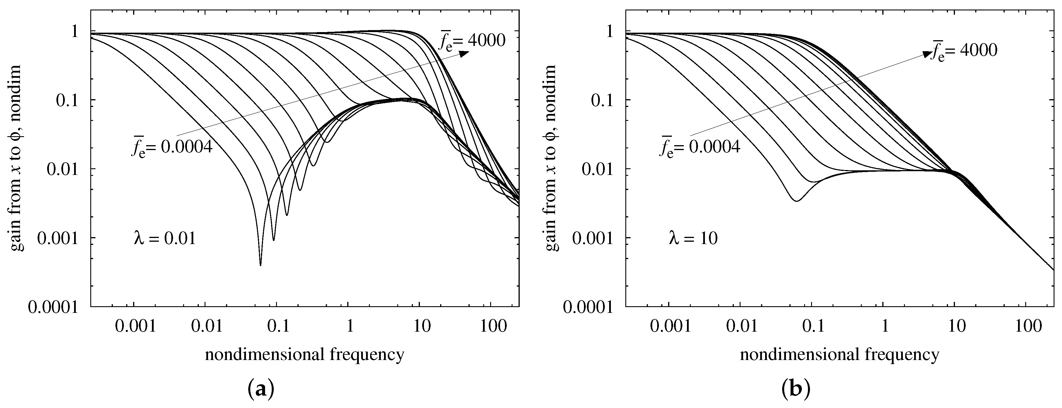
The first input-output frequency response function used to compare the relative performance of transconductance and transpermeance amplifiers is the relationship between non-dimensional rotor displacement () and non-dimensional flux (). Figure 3 depicts this relationship under amplifier variation (), with and without eddy current effects. The results shown in Figure 3 demonstrate that a transpermeance amplifier dramatically reduces the bandwidth of the influence of displacement on the actual flux (corresponding to a reduced negative mechanical stiffness () effect). The bandwidth is also affected by eddy currents: strong eddy current effects reduce the bandwidth of this influence. With transpermeance, there is a frequency range where there is some recovery of the influence of displacement, converging to the transconductance influence at high frequencies. This region has a plateau gain that depends on the level of eddy currents. With no eddy currents, the plateau is roughly a factor of 10 lower than with transconductance, while with strong eddy currents, the plateau is roughly a factor of 100 lower than with transconductance.
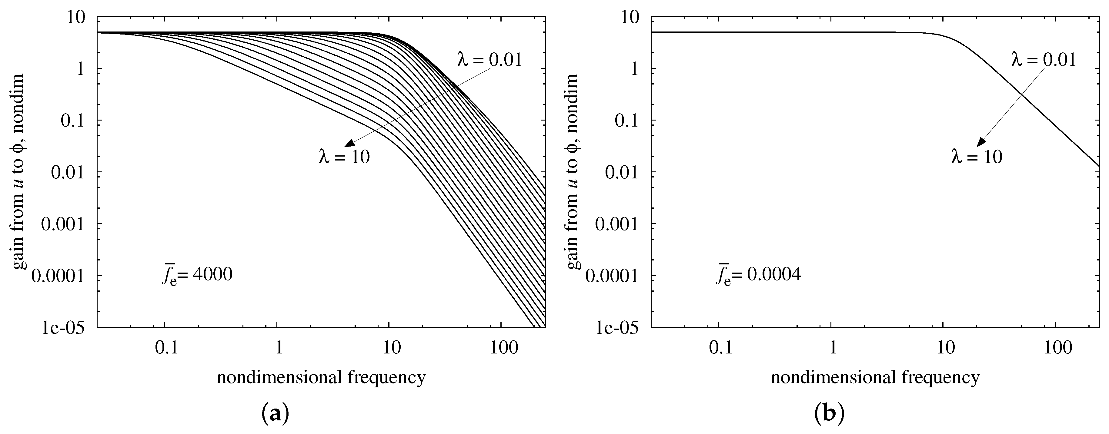
Next, the response between the non-dimensional command voltage () and non-dimensional flux () is studied for varying levels of eddy currents (Figure 4). Figure 4a demonstrates that with transconductance, the actuator loses bandwidth dramatically with increasing eddy current effect, while with transpermeance (shown in Figure 4b), eddy currents have essentially no effect on actuator bandwidth. This dramatic flux (force) bandwidth improvement for transpermeance amplifiers under the influence of eddy currents is especially noteworthy, and the way in which this performance improvement is achieved deserves further investigation.
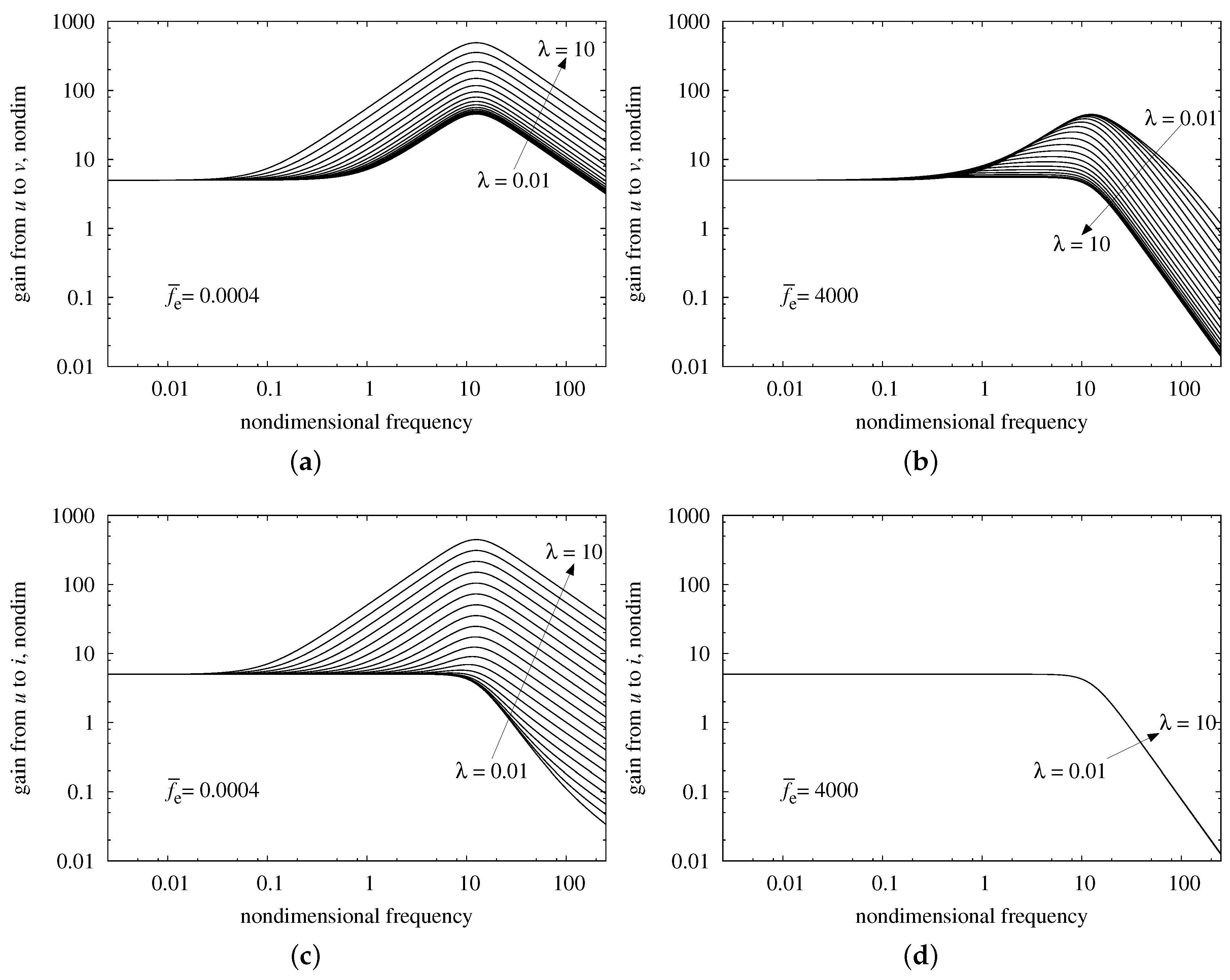
Figure 5 presents a comparison between transpermeance and transconductance amplifiers with and without eddy current effects from the perspective of non-dimensional command voltage () to the non-dimensional required actuator voltage () and current (). Figure 5 illustrates that, for actuators with negligible eddy currents, the required voltage and current are similar for transpermeance and transconductance amplifiers. However, under strong eddy currents, the required voltage and current behavior is significantly different for transpermeance and transconductance amplifiers. At low non-dimensional frequencies (<0.01), the required voltage and current are similar for both amplifier types, as well as being identical to requirements when no eddy currents are present. However, at higher frequencies, the transpermeance amplifier requires a significantly higher peak voltage, approximately a 10× increase compared to the peak requirements for transpermeance and transconductance without eddy currents (refer to Figure 5a). In addition, it is interesting to note that the coil voltage under strong eddy currents for a transconductance amplifier is actually lower than that associated with low eddy current operation (Figure 5b). Turning to the required coil currents for transpermeance amplifiers under strong eddy currents, it can be seen from Figure 5c that the required peak current levels are approximately 100× those required for low eddy current operation. These higher peak voltage and current are required in order to overcome the eddy current effects and, thus, achieve the same flux (force) bandwidth as systems with low eddy current actuators.
For transconductance operation, the coil current for low and high eddy currents is unchanged (refer to Figure 5d). This is due to the fact that under transconductance operation, the eddy current effects are unobservable, and therefore, current levels remain unchanged, resulting in the significant flux (force) bandwidth reduction seen in Figure 4a.
From a practical perspective, the higher peak voltage and current required by transpermeance operation to achieve the significantly higher flux (force) bandwidth in the presence of strong eddy currents should not significantly impact the small signal bandwidth capability of an actual closed loop amplifier-actuator system. For medium to large signals, although bandwidth improvements will still exist, they will be less than that predicted in this study due to non-linear saturation effects associated with the amplifier hardware.
4.3. Transient Response Simulation
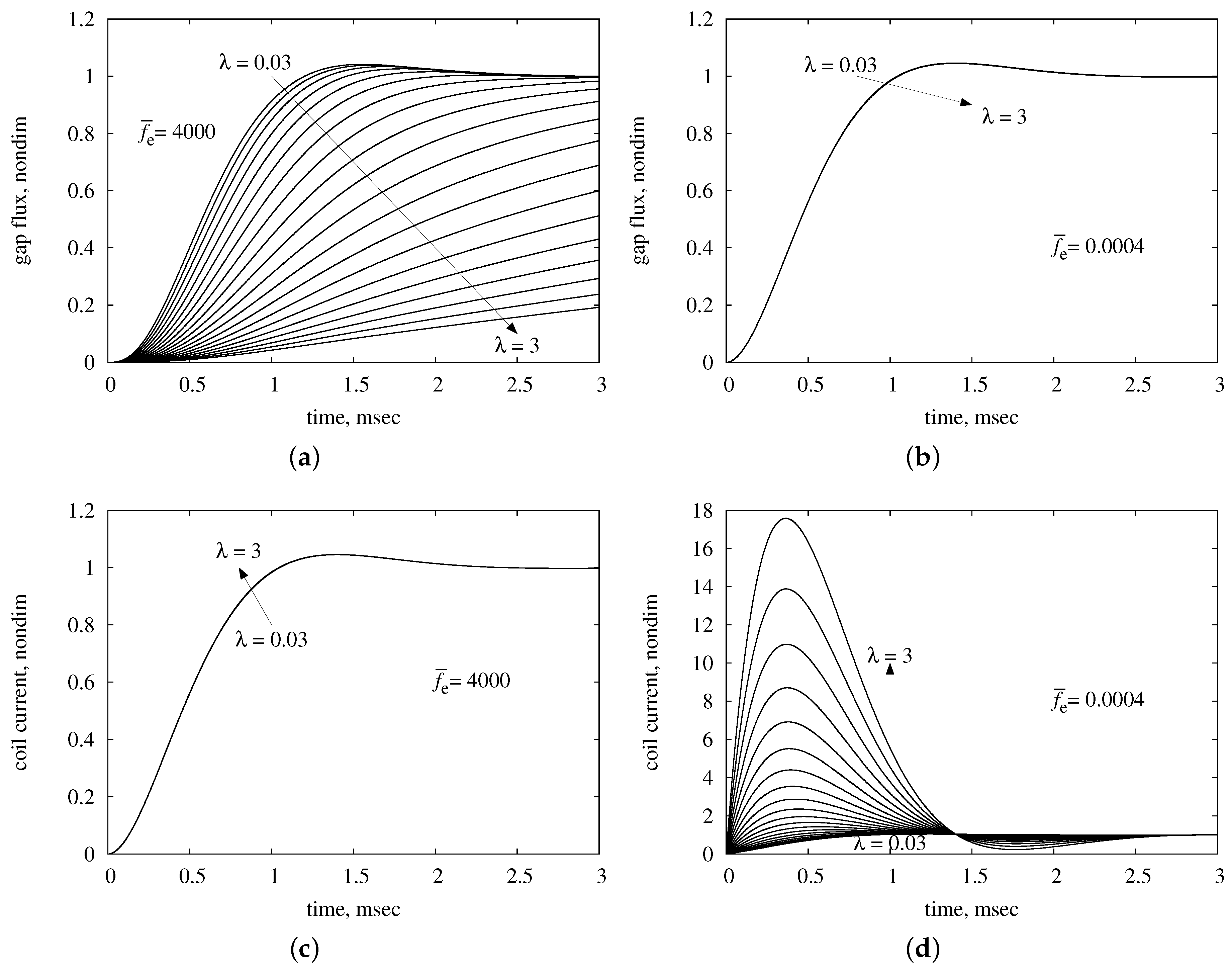
To see the behavior of the two amplifier schemes in more physical terms, step response simulations were performed for a step input to the amplifier command. Figure 6 depicts the step response of gap flux, coil current and coil voltage for transconductance and transpermeance amplifiers. The amplifier input signal step was chosen to produce a change in gap flux equal to the mean gap flux, , so the non-dimensional response is 1.0. The non-dimensional current and voltage responses follow suit, each reaching a steady state value of 1.0 corresponding to a change in coil current equal to the mean current, , and a change in coil voltage equal to the mean voltage, .
Figure 6c illustrates the current response of a transconductance amplifier (). Regardless of the level of eddy current production (λ ranges from 0.03 to three in the figure), the response is the same: the amplifier is designed for this response.
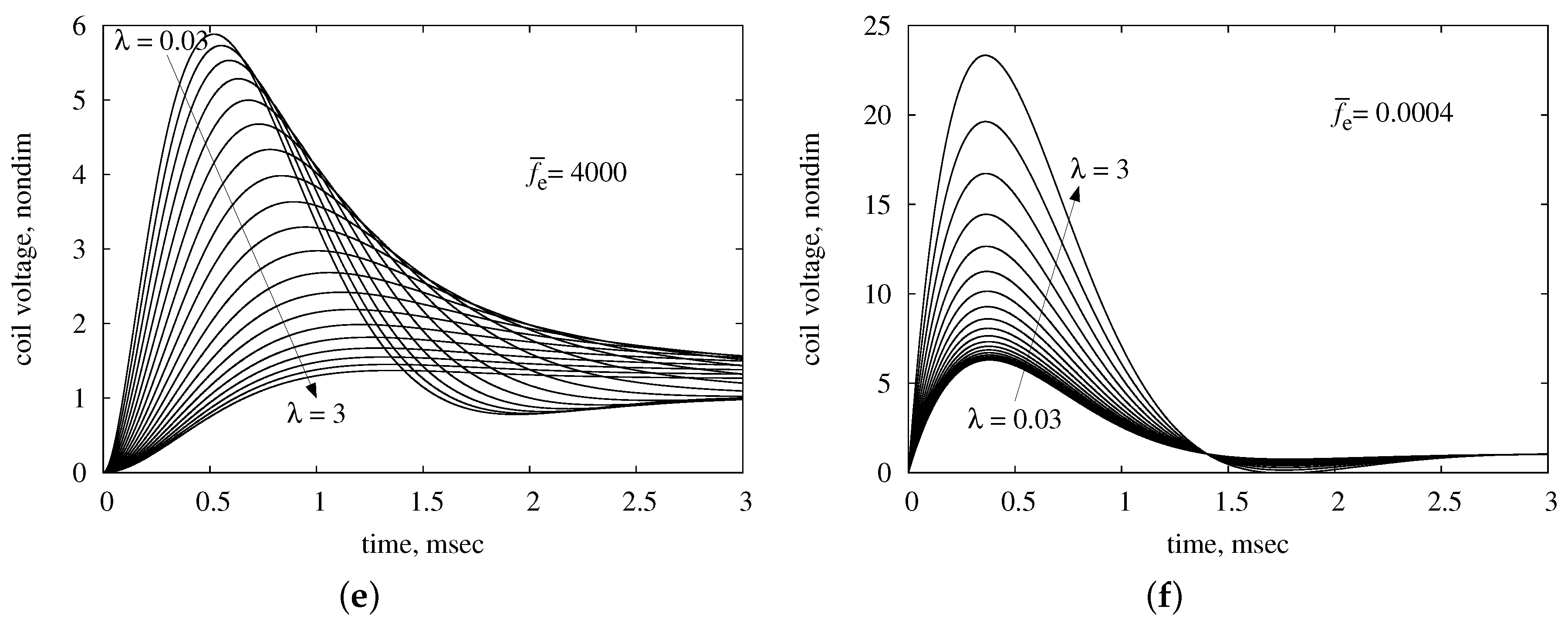
Figure 6a shows the corresponding gap flux response, and it is clear that, with very little eddy current effect (), the flux tracks the current, reaching a peak at about 1.3 ms. On the other hand, as the eddy currents become progressively stronger (), the flux response becomes more and more sluggish. Figure 6e illustrates the coil voltage required to achieve this current and flux response. As expected, the voltage is high when the flux is increasing rapidly, and the peak voltage is about six-times larger than the steady state voltage when eddy currents are negligible. At high levels of eddy current production, the peak voltage is much lower because the rate of flux change is so low.
The picture changes substantially when a transpermeance amplifier () is used instead of a transconductance amplifier. As Figure 6b shows, the gap flux response is now essentially invariant as the level of eddy current effect changes, instead of the current as with a transconductance amplifier. On the other hand, the current response shown in Figure 6d now depends strongly on the level of eddy currents, showing a large peak current when the eddy currents are very strong. This peak current is needed to cancel the effect of the eddy currents. The coil voltage needed to achieve this flux and current response is illustrated in Figure 6f. Here, the large initial peak voltage associated with high eddy currents () is largely due to the large initial excess current needed to cover the eddy current production: without the eddy currents, the peak would only be about six-times the steady state change, as with transconductance in the absence of eddy currents.
4.4. Comments on Simplifications
Finally, although this study is based on a relatively simple eddy current model and it is a theoretical, as opposed to an experimental, study of the relative performance of transpermeance versus transconductance amplifiers, the authors hypothesize that the overall trends of this study should still hold for actual systems. This hypothesis is based on the fact that the model used in this study, although relatively simplistic, deviates from more accurate models primarily at higher frequencies where the transpermeance model pays no attention to the current signal. In addition, one of the primary shortcomings of the simple eddy current model used in this work is its inability to capture the skin effect and associated high frequency magnetic field leakage. The skin effect is investigated in the next section in an attempt to better understand the impact of this effect on the overall performance-related trends discussed above.
5. Skin Effect
One of the possible limitations to the apparent bandwidth advantage of transpermeance amplifiers when the actuator is susceptible to substantial eddy currents arises because of the skin effect. The skin effect is a consequence of the fact that eddy currents arise throughout the volume of the electrically-conductive magnetic material, and this means that they tend to exclude the magnetic field from the core and push it toward the perimeter of the material. An underlying assumption of the argument that transpermeance extends the actuator bandwidth is that the pole force is proportional to the square of the total pole flux. Obviously, this is a simplification of Maxwell’s stress tensor, which says (approximately) that the force is given by the surface integral of the square of the flux density. If the flux density is essentially uniform over the pole surface, then the assumption that force is proportional to the square of total flux is a good one, but the skin effect challenges this.
To see how the skin effect might alter the relationship, consider a very simple model where the pole area is broken into two regions, and : , and that the flux density over each of these two regions is perfectly uniform: in area and in area . In this manner, the total pole flux is . Now, consider the relationship between the actual force, f, and that estimated by the assumption that force is proportional to the square of the total pole flux, :
so that:
If , then , and remarkably, the assumption that force is proportional to the square of total pole flux underestimates the actual force. In fact, , except in the case that , in which case the two terms are equal. Therefore, this means that using the square of the total pole flux as a proxy for pole force is actually conservative.
To see this, assume that and β can take on any positive value. In this case,
The quadratic function is an upward parabola with at (repeated root). Hence, for all real values of β, , which means that:
This argument can be readily extended to the case where B is some function of spatial variables across the surface of the pole face, . In this case,
It is a bit involved, but reasonably straightforward to prove that:
which supports the argument in the more general case.
6. Conclusions
Before discussing the possible merits of transpermeance amplifiers for active magnetic bearings, it is important to point out that transpermeance as presented here is very easy to accomplish. In contrast to conventional transconductance amplifiers, which require high bandwidth feedback of the coil current and therefore relatively low-noise measurement of current, a transpermeance amplifier uses low bandwidth feedback both of coil current and of coil voltage. Therefore, the requirements for coil current measurement are easier to meet, and the measurement of coil voltage can be as simple as measuring the PWM duty cycle and multiplying by measured bus voltage: the voltage need not be measured directly. Setting aside the issue that off-the-shelf servo drives (as are often used as the power amplifier in AMB systems) require some modification to support transpermeance, the measurement and estimator construction are undemanding. Even off-the-shelf servo drives can support this if they provide for a voltage feedback mode.
Two effects were examined in the present work: the negative mechanical stiffness () associated with AMBs that is responsible for the static instability fundamental to the technology and the effect of eddy currents. It is certainly the case that using transpermeance offers a means to reduce the bandwidth of the term, and this may broaden the controller design space in some AMB applications. While it must be conceded that the instability associated with is typically not the hardest to overcome in the AMB design process, it does set a minimum closed loop stiffness requirement for robust stability, and this then limits the range of controller design choices. This could be especially significant in applications that favor a soft bearing, such as flywheels.
An interesting feature of this bandwidth reduction is the plateau noted in Figure 3 that effectively limits the reduction to a factor of about ten over a wide frequency range. This plateau may be a consequence of the particular estimator weighting function, , used to produce the parametric study or it may be a consequence of the physics of the problem; it certainly merits further investigation.
The exploration of eddy currents presented here shows that a simple model for eddy currents predicts a loss of actuator bandwidth when a transconductance amplifier is used. While the model is perhaps overly simplistic, this conclusion is supported by experiments and other more sophisticated analyses in the literature. When a transpermeance amplifier is substituted, the present analysis predicts substantial gains in bandwidth, but at the cost of higher voltage and current requirements to cover the effect of the eddy currents. Whether or not this observation is correct depends to some extent on the fidelity of the eddy current model: admittedly, the present model is not good enough to claim this advantage with high confidence. However, the result does suggest that transpermeance amplifiers are likely to provide higher bandwidth when the magnets exhibit eddy currents, so this prospect bears further exploration either using better eddy current models or through physical experimentation.
In conducting further exploration of eddy currents, there are three issues that particularly bear focus. First is the simple fidelity of the model. Numerous better models are available, and many have been supported with experimental evidence, so they could be implemented in simulation with fairly high confidence. Perhaps more important, however, is the influence of the skin effect on the relationship between total pole flux and generated force. In non-laminated actuators, such as are commonly implemented for thrust bearings and where eddy current effects are particularly important, the skin effect is likely to produce a frequency-dependent relationship between total pole flux (as estimated by a transpermeance amplifier’s flux estimator) and the resulting pole force. Arguably, this relationship actually means that the flux estimate under-estimates the actual force, so this effect is somewhat to the advantage of a transpermeance amplifier, but this point certainly requires further investigation if the potential advantage to AMB thrust bearings is to be exploited. Finally, a central assumption in transpermeance is that the flux linked by the magnet drive coil equals the flux passing through the pole face. Of course, this neglects magnetic leakage effects. While leakage is typically small when the material is not saturated, it is certainly never zero and, in particular, is stronger when the field is compressed to the material perimeter by eddy currents. Hence, the flux linked by the drive coil always overestimates the flux passing through the pole face and is responsible for generating bearing forces, and this overestimation is probably exacerbated by eddy currents. This would push the flux estimate of force toward overprediction.
While the most important issues to consider when contemplating a switch from transconductance to transpermeance seem to be bandwidth in the face of eddy current effects and suppression of negative magnetic stiffness effects, it is likely that numerous other issues will prove relevant. In particular, static offset error in estimating gap flux may present significant complications to both schemes, but may manifest differently. Further, although the low bandwidth sensing requirements are touted here as an advantage, the actual effects of measurement noise have not been explicitly examined and may, again, produce different problems in the two approaches. Finally, nonlinearities, such as PWM switching of the power electronics converters, amplifier current saturation and actuator magnetic material saturation, will have an impact on the behavior of both amplifier architectures; however, they were not included in this present study due to the linear nature of the analysis techniques used here. Clearly, all of the above issues should be investigated in future work on this problem.
In balance, given the ease with which transpermeance can be implemented and given the advantages provided by this approach, it seems clear that transpermeance should replace transconductance as the preferred amplifier mode for AMB applications.
Acknowledgments
This work was funded in part by a postdoctoral research grant from the government of Brazil. Additional support was provided by the Rotating Machinery and Controls Laboratory (ROMAC) at the University of Virginia.
Author Contributions
Both the research for this paper and the writing of the paper were performed jointly by all three authors.
Conflicts of Interest
The authors declare no conflict of interest.
References
- Aenis, M.; Nordmann, R. A precise force measurement in magnetic bearings for diagnosis purposes. In Proceeding of the Fifth International Symposium on Magnetic Suspension Technology, Santa Barbara, CA, USA, 1–3 December 1999; pp. 397–410.
- Cao, G.; Lee, C.W. Development of PWM power amplifier for active magnetic bearings. In Proceedings of the Fifth World Congress on Intelligent Control and Automation, Hangzhou, China, 15–19 June 2004; Volume 4, pp. 3475–3478.
- Bleuler, H.; Cole, M.; Keogh, P.; Larsonneur, R.; Maslen, E.; Nordmann, R.; Okada, Y.; Schweitzer, G.; Traxler, A. Magnetic Bearings: Theory, Design, and Application to Rotating Machinery; Schweitzer, G., Maslen, E.H., Eds.; Springer: Berlin/Heidelberg, Germany, 2009. [Google Scholar]
- Keith, F.J. Implicit Flux Feedback Control for Magnetic Bearings. Ph.D. Thesis, University of Virginia, Charlottesville, VA, USA, 1993. [Google Scholar]
- Groom, N.J. A Magnetic Bearing Control Approach Using Flux Feedback; NASA-TM-100672; NASA Technical Reports Server: Hampton, VA, USA, 1989. [Google Scholar]
- Jastrzȩbski, R.P.; Smirnov, A.; Mystkowski, A.; Pyrhönen, O. Cascaded position-flux controller for an AMB system operating at zero bias. Energies 2014, 7, 3561–3575. [Google Scholar] [CrossRef]
- Zhu, L.; Knospe, C.R.; Maslen, E. Analytical model for a nonlaminated cylindrical magnetic actuator including eddy currents. IEEE Trans. Magn. 2005, 41, 1248–1258. [Google Scholar]
- Zhu, L.; Knospe, C.R.; Maslen, E.H. Frequency domain modeling of non-laminated cylindrical magnetic actuators. In Proceedings of the 9th International Symposium on Magnetic Bearings, Lexington, KY, USA, 3–6 August 2004.
- Zhu, L.; Knospe, C.R. Modeling of nonlaminated electromagnetic suspension systems. IEEE/ASME Trans. Mechatron. 2010, 15, 59–69. [Google Scholar]
- Whitlow, Z.W.; Fittro, R.L.; Knospe, C.R. Dynamic Performance of Segmented Active Magnetic Thrust Bearings. IEEE Trans. Magn. 2016, 52. [Google Scholar] [CrossRef]
- Zhou, L.; Li, L. Modeling and Identification of a Solid-Core Active Magnetic Bearing Including Eddy Currents. IEEE/ASME Trans. Mechatron. 2016, 21, 2784–2792. [Google Scholar] [CrossRef]
- Zmood, R.B.; Anand, D.K.; Kirk, J.A. The Influence of Eddy Currents on Magnetic Actuator Performance. Proc. IEEE 1987, 75, 259–260. [Google Scholar] [CrossRef]
- Feeley, J.J.; Ahlstrom, D.J. A New Eddy Current Model for Magnetic Bearing Control System Design. In Proceedings of the 4th NASA Symposium on VLSI Design, Moscow, Russia, 29–30 October 1992.
- Johnson, D.; Brown, G.V.; Inman, D.J. Adaptive variable bias magnetic bearing control. In Proceedings of the 1998 American Control Conference, Philadelphia, PA, USA, 26 June 1998; Volume 4, pp. 2217–2223.
Figure 1.
Generalized amplifier architecture.

Figure 2.
Actuator and eddy current windings.
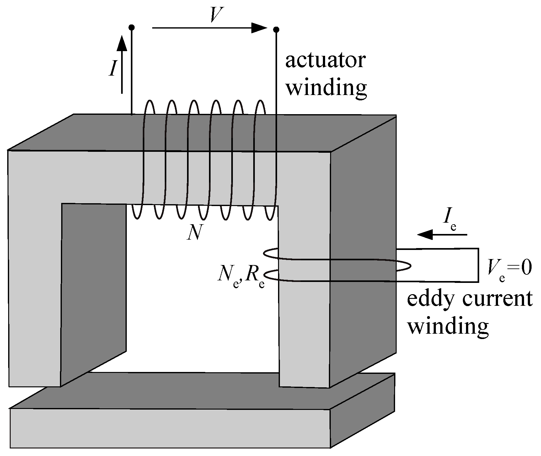
Figure 3.
Frequency response under amplifier variation with and without eddy current effects. (a) Gain from rotor displacement to flux without eddy current effects (); (b) gain from rotor displacement to flux with strong eddy current effects ().
Figure 3.
Frequency response under amplifier variation with and without eddy current effects. (a) Gain from rotor displacement to flux without eddy current effects (); (b) gain from rotor displacement to flux with strong eddy current effects ().

Figure 4.
Frequency response of transconductance and transpermeance amplifiers under λ variation. (a) Gain from command voltage to flux: transconductance () ; (b) gain from command voltage to flux: transpermeance ().
Figure 4.
Frequency response of transconductance and transpermeance amplifiers under λ variation. (a) Gain from command voltage to flux: transconductance () ; (b) gain from command voltage to flux: transpermeance ().

Figure 5.
Frequency response of transpermeance and transconductance amplifiers under eddy current effects variation. (a) Gain from command voltage to coil voltage: transpermeance (); (b) gain from command voltage to coil voltage: transconductance (); (c) gain from command voltage to coil current: transpermeance (); (d) gain from command voltage to coil current: transconductance ().

Figure 6.
Step responses of the electromagnet-amplifier combination, showing a range of eddy current levels. In the left column are responses for transconductance amplifiers (), and in the right column are responses for transpermeance amplifiers (). The step size was chosen to produce a step change in flux equal to the initial mean flux, . (a) Change in non-dimensional gap flux versus time; (b) change in non-dimensional gap flux versus time; (c) change in non-dimensional coil current versus time; (d) change in non-dimensional coil current versus time; (e) change in non-dimensional coil voltage versus time; (f) change in non-dimensional coil voltage versus time.


| A | pole cross-section area | AMB mechanical stiffness, | |
| arbitrary polynomial in s | L | inductance | |
| state evolution matrix of amplifier controller | iron path length | ||
| flux estimator state evolution matrix | N | number of coil turns | |
| composite state evolution matrix | effective turns of eddy current circuit | ||
| arbitrary polynomial in s | q | outputs of the magnetic model | |
| magnetic flux densities | R | coil resistance | |
| flux estimator input matrices | states of amplifier controller | ||
| input matrix of amplifier controller | flux estimator states | ||
| voltage input matrix to the composite model | states of the composite model: ϕ and | ||
| displacement input matrix to the composite model | s | argument of the Laplace transform | |
| output matrix of amplifier controller | t | time | |
| flux estimator output matrix | u | amplifier reference voltage | |
| output matrix of the composite model | V | coil voltage | |
| estimated flux output matrix of the composite model | v | perturbation coil voltage, | |
| differential unit of area | mean coil voltage | ||
| feed–through matrix of amplifier controller | estimator weighting function | ||
| voltage feed-through matrix of the composite model | x | rotor displacement | |
| x feed-through matrix of the composite model | mean value of x (assumed zero) | ||
| f | forced generated by magnetic quadrant | α | |
| estimator cross-over frequency | β | flux density ratio | |
| amplifier bandwidth | λ | eddy current parameter | |
| g | actual air gap | permeability of the air | |
| average air gap | relative permeability | ||
| transfer function from current to flux | ξ | amplifier damping ratio target | |
| magnetic transfer function from V and x to Φ and I | flux estimator time constant | ||
| amplifier target dynamics | magnetic time constant | ||
| forward amplifier gain from u to V | Φ | actuator gap magnetic flux | |
| transfer function from coil voltage to flux | estimated magnetic flux | ||
| feedback gain on estimated flux | ϕ | perturbation flux, | |
| transfer function from v to | estimated perturbation flux | ||
| transfer function from u to | mean gap magnetic flux | ||
| I | coil current | flux estimate for high frequencies | |
| i | perturbation current: | flux estimate for low frequencies | |
| mean value of coil current | saturation magnetic flux | ||
| eddy current | amplifier bandwidth target | ||
| AMB actuator gain, | non-dimensional version of variable h |
© 2017 by the authors. Licensee MDPI, Basel, Switzerland. This article is an open access article distributed under the terms and conditions of the Creative Commons Attribution (CC BY) license ( http://creativecommons.org/licenses/by/4.0/).
Share and Cite
MDPI and ACS Style
Ferreira, J.; Maslen, E.; Fittro, R. Transpermeance Amplifier Applied to Magnetic Bearings. Actuators 2017, 6, 9. https://doi.org/10.3390/act6010009
AMA Style
Ferreira J, Maslen E, Fittro R. Transpermeance Amplifier Applied to Magnetic Bearings. Actuators. 2017; 6(1):9. https://doi.org/10.3390/act6010009
Chicago/Turabian StyleFerreira, Jossana, Eric Maslen, and Roger Fittro. 2017. "Transpermeance Amplifier Applied to Magnetic Bearings" Actuators 6, no. 1: 9. https://doi.org/10.3390/act6010009
Note that from the first issue of 2016, this journal uses article numbers instead of page numbers. See further details here.