
A System Identification Technique Using Bias Current Perturbation for the Determination of the Magnetic Axes of an Active Magnetic Bearing

1
Joseph F. Ware, Jr. Advanced Engineering Lab, College of Engineering, Virginia Tech, Blacksburg, VA 24061, USA
2
Department of Engineering, James Madison University, Harrisonburg, VA 22807, USA
3
Department of Mechanical Engineering, Virginia Tech, Blacksburg, VA 24061, USA
*
Author to whom correspondence should be addressed.
Actuators 2017, 6(2), 13; https://doi.org/10.3390/act6020013
Submission received: 14 December 2016
/
Revised: 8 February 2017
/
Accepted: 2 March 2017
/
Published: 28 March 2017
(This article belongs to the Special Issue Active Magnetic Bearing Actuators)
Abstract
:Inherent in every Active Magnetic Bearing (AMB) are differences between the expected geometric axes and the actual magnetic axes due to a combination of discrepancies, including physical variation from manufacturing tolerances and misalignment from mechanical assembly, fringing and leakage effects, as well as variations in magnetic material properties within a single AMB. A method is presented here for locating the magnetic axes of an AMB that will facilitate the accurate characterization of the bearing air gaps for potential improvement in field tuning, performance analyses and certain shaft force measurement techniques. This paper presents an extension of the application of the bias current perturbation method for the determination of the magnetic center to the determination of magnetic axes for the further development of accurate current-based force measurement techniques.
1. Introduction
Active Magnetic Bearings (AMBs) have the ability to concurrently provide load-carrying support for rotating machinery and serve as a non-invasive shaft force sensor. During operation, a magnetic field that is developed in an AMB’s stator serves to support the rotor, resulting in rotor levitation with no physical contact between bearing components. By modeling the magnetic flux between stator and rotor, the force necessary for rotor support may be predicted in real time [1]. While the physics associated with active magnetic bearing performance are understood well enough to result in successful bearing designs using broad assumptions and factors of safety, more precise information about the parameters associated with the final field installation of an AMB are required for the development of high accuracy real-time shaft force techniques utilizing bearing currents. Manufacturing and installation of an AMB can result in myriad parameters that affect the actual air gaps at specific points, and these parameters are not specifically known, nor are they directly measurable. Successful modeling of the magnetic flux relies on the knowledge of current in the coils of the stator-based electromagnets and the air gap length between the rotor and stator. Assuming that an air gap is equal to the designated air gap from the manufacturing specifications limits the accuracy of determined shaft forces because differences between magnetic flux calculated from a current-based model and the actual magnetic flux within the air gap exist due to unmodeled behavior, including misalignment, material inhomogeneity, out-of-roundness, flux leakage and flux fringing, among other parameters. If left unaddressed, the effect of these differences on force measurement can be significant. This paper describes an approach that relies on observed AMB behavior at a relatively small number of selected points to develop an air gap correction by which the geometrically-determined air gap is replaced with an “effective” air gap that accounts for variations between theoretical model predictions and experimental observations, thus providing an effective magnetic center and axes for use in determining accurate current-based force measurements. The model was developed specifically as a way to improve AMB force predictions without the requirement for additional hardware; as such, it may be extended to other field-based diagnostics related to the evaluation of magnetic flux properties. Modeling of the effective air gap is intended as a diagnostic tool to promote accurate current-based force measurements; it is not intended to suggest an optimum physical operating point.
The work presented here leverages previous efforts of Prins, which are based on a system identification technique that employs perturbation of bias current, referred to as the Multi-Point Method (MPM), as developed by Marshall, Kasarda and Imlach [1]. Prins [2,3] showed that the MPM could be used to establish the location of an “effective origin” that differs from the systems’ geometric origin, an important step in characterizing the bearing gap. Prins [2] did a pilot study extending that work to additionally characterize a set of “effective axes” that differed from the systems’ geometric axes, allowing the favorable force measurement results observed at the effective origin to be realized throughout the rotor space. The preliminary work done by Prins [2] is extended here to demonstrate the viability of the approach over a larger range of bias currents and spatial parameters and to consolidate the observed differences between effective and system coordinates through the use of an “error vector,” εn. The technique analyzes the AMB system’s response to the perturbation of bias currents in conjunction with a magnetic circuit model to infer the center and axes positions. The end result of the technique is a set of transformation equations that map the geometric coordinates reported by the AMB system to an effective coordinate system. Once the transformation equations are established, bias perturbation is no longer necessary and an analytical approach to system identification of the bearing’s magnetic field results.
Literature Review
A synopsis of modern active magnetic bearing technologies is provided by Kasarda [4]. In this work, various applications are discussed, including centrifugal and turbo molecular pumps, X-ray tube mounts in CAT scanners and supports for high-speed centrifugal neutron choppers used in nuclear research. Kasarda [4] reports that one of the most promising applications of magnetic bearings includes manufacturing scenarios, because of the ability of AMBs to provide non-invasive force sensing.
Multiple researchers have investigated approaches for exploiting the force measurement capability of AMBs. Gahler and Forch [5] describe a mathematical method of force measurement for an eight pole hetero-polar magnetic bearing. Their work involves the addition of Hall effect sensors to measure magnetic flux between the bearing’s stator and rotor. This allows for the measurement of force for each perpendicular bearing axis via a magnetic resistor network. They use their measured magnetic flux in a magnetic force model for the bearing to determine bearing loads. While their work also utilizes a magnetic force model approach, they require the use of additional delicate hardware that may be impractical in a field application.
Rantatalo et al. [6] employ Contact-less Dynamic Spindle Testing equipment (CDST) to analyze machine tool spindle vibrations. The CDST measures frequency response functions of a tool tip by exciting the rotor with electromagnets and determining applied force from bearing currents. CDST frequency measurements deviated from a traditional tap test (both measured at 0 rpm) possibly due to changes in spindle location.
Examination of cutting forces in high speed machining provides a way to estimate tool wear and to assess product quality. Auchet et al. [7] use active magnetic bearings to measure cutting forces for a five-axis milling machine by examining AMB command voltages. Results from the AMBs are compared to those obtained from a Kistler dynamometer. Combining data from the outboard and inboard AMB via a least squares method, cutting force amplitudes are adequately predicted compared to those from the dynamometer. Operational speeds of 10,000, 11,000 and 14,000 rpm were considered.
Similar to [6], Aenis et al. [8] use AMBs to measure frequency responses for a centrifugal pump. An i-s (current–displacement) force measurement method using an inboard and outboard AMB is compared to results obtained from a reluctance network approach and a flux-based method requiring up to eight Hall sensor probes. The i-s approach produces results with an 8% error at maximum applied bearing force for a concentric rotor and 9% for an eccentric rotor. Using Hall sensors, the error is reduced to about a 1% range (concentric case) to 5% (eccentric case). Aenis reports that force errors from the Hall sensors can be reduced to 2.5% by accounting for offset errors in the eccentric rotor position.
Permanent Magnets (PM) are used by Hussien et al. [9] in conjunction with controlled electromagnets for facilitating a mechanical balance system. Permanent repulsive-type magnetic bearings stabilize the radial (z-axis) direction, simplifying the control of the axial (x) and perpendicular radial (y) directions. The mechanical balance system (not directly utilizing magnetic bearing data) results in errors less than 0.2% at a maximum load of 100 mg.
Marshall, Kasarda and Imlach [1] recognized the opportunity to exploit the behavior of the active magnetic bearing control system to develop a system identification approach for determining effective magnetic gaps. Experimentally-determined effective magnetic gaps have the potential to be used in magnetic force equations, in conjunction with electric actuator current, to provide a more accurate measurement of the force applied by the bearing to support the shaft. This system identification method, called the Multi-Point Method (MPM), perturbs the system by adding an additional amount of current to a set of actuators and then takes advantage of the feedback feature of AMB systems in maintaining a supported rotor shaft at the rotor set point location. By equating the magnetic force equations at the different perturbations, or multiple points, during the system identification test, the effective gap values are determined [2]. This experimentally-determined effective magnetic gap likely accounts for simplifying assumptions used in determining the magnetic force model. For example, the force model of magnetic bearings does not account for variations in an actual bearing-rotor system, such as misalignment between rotor and stator, variations in geometry or material properties, temperature effects and magnetic fringing and leakage, among other possible scenarios, that can impact the actual field setup and performance of the AMB. While “rule of thumb” correction factors can be used, the MPM potentially allows for a way of experimentally accounting for these unknowns in any AMB-supported rotor system by determining “effective” gaps.
Prins [3] demonstrates how the multi-point method could be used to identify an effective origin that differs from the controller-reported geometric origin. Prins [2] also describes an extension of that approach in which the controller-reported geometric coordinates that describe the AMB working space are remapped to an effective coordinate system that is offset, rotated and scaled relative to controller-reported geometric coordinates. In that study, variations between model prediction of static bearing reaction force and transducer-based reaction force measurements for five different AMB systems ranged from 3%–22% of measured load when controller-reported geometric coordinates were used in the force prediction model. Application of effective coordinates to the force prediction models resulted in a reduction of variation to 2%–6% of measured load.
2. Materials and Methods
2.1. The Multi-Point Method System Identification Approach
The work presented here for determining the effective magnetic axes is based on the MPM discussed earlier [1,2,3]. Shown in Figure 1 is a simplified version of a single axis of a magnetic bearing-rotor system. Top and bottom currents (itop and ibottom) are recorded once the rotor is stabilized to establish an initial data point. Multiple data points are obtained by increasing current via small incremental changes in bias, thus “perturbing” the system.
The method exploits the fact that the support current in each actuator will be determined based on controller action to maintain rotor levitation after perturbation current is added to the system. After bias current perturbation, new resulting current values for top and bottom actuators, respectively, are obtained providing an additional data point. By repeating this procedure, a series of data points is determined, establishing a functional relationship between magnetic force and rotor position. For two actuators with a vertical orientation, the net magnetic force applied to the rotor is [10]:
where gtop and gbottom are functions of rotor position and are calculated as:
where go is the nominal (manufacturer’s) air gap, and x is the displacement of the target from the bearing’s effective center. For a given geometry, material and coil current, Equation (1) has two unknowns, Fmagnetic and x. The MPM method recognizes that separate current datasets that result from modification of the bias current must correspond to the same bearing force and rotor position due to the control system. For any two pairs of equations, a single unknown value x may be determined that corresponds to the same reaction, or force, at the same rotor position set point. Consider input bias setting ibias,1 resulting in output currents (itop,1, ibottom,1). Substitution of currents into Equation (1) leads to:
A second independent equation results for a second bias setting (ibias,2), where we assume ibias,2 > ibias,1:
Since the bearing reaction does not change as bias current is changed, or perturbed, F1 = F2, therefore [3]:
Mathematically, two solutions exist in Equation (8), but only one real solution corresponding to ibias2 > ibias1 occurs [3]. The cosine term in Equation (8) accounts for horseshoe pairs oriented at an angle θ′ from the vertical.
F1 and F2 are each equal to the actual magnetic bearing force applied to the rotor to keep it levitated at the rotor position set point. Using the modified approach, Prins reports bearing reaction forces applied to the shaft with measurement accuracies within 3% in a stationary rotor [2].
2.2. Experimental Approach
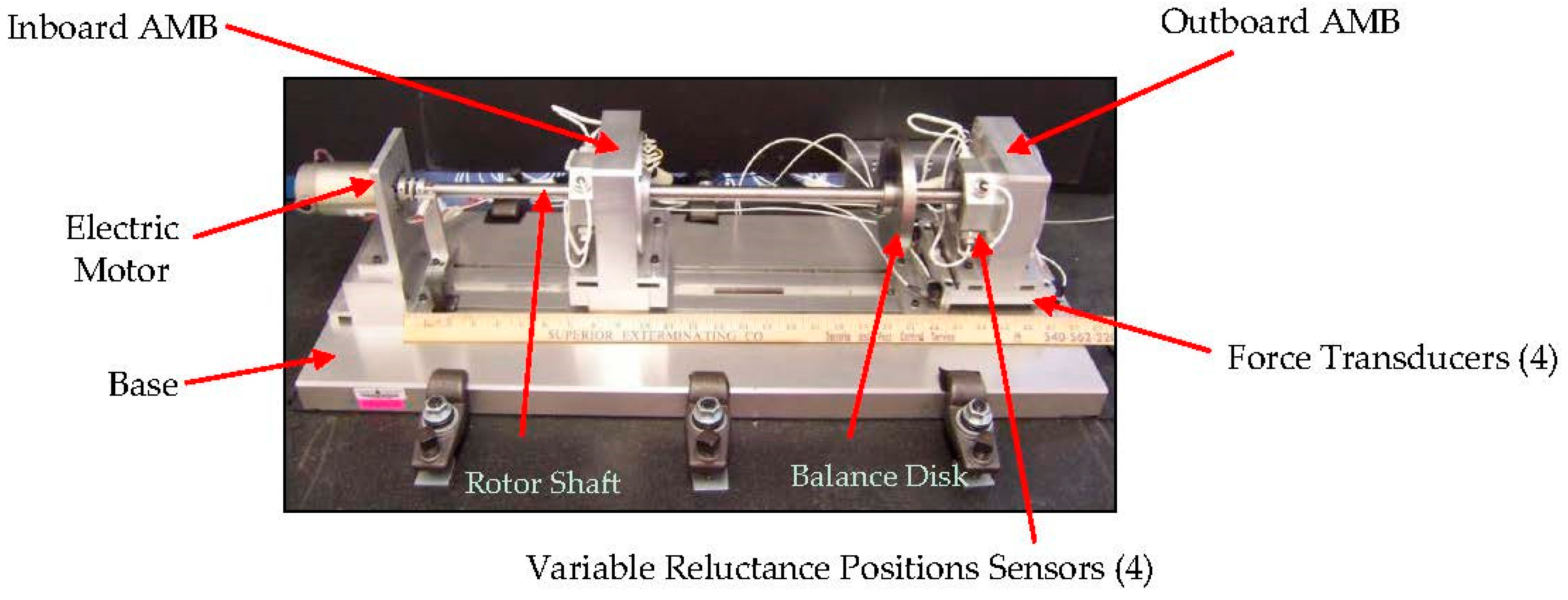
Figure 2 illustrates the rotor test stand configuration used in this study consisting of inboard and outboard hetero-polar AMBs, rotor shaft, balance disk, variable reluctance position sensors, force transducers and electric motor. The entire assembly rests on a rubber pad and 1500-pound base, which provides ambient vibration isolation [12].
The rotor shaft has a free span of 0.4064 m, the radius of the bearing rotor is 7.94 mm, and the stator and rotor have a nominal diametric gap of 762 µm. It is determined experimentally that the radial clearance between rotor shaft and catcher bearing is 144 µm [11]. The catcher bearing provides a surface in case of loss of magnetic levitation and ensures that the rotor does not come into contact with the stator pole face.
2.3. Experimental Signal Flow
PID control allows for rotor placement at locations specified by set points via signals from the four position sensors. Voltage signals from controller and position sensors are sent to an NI DAQ board. Signals from each of the four PCB™ force transducers located under the outboard bearing are also recorded. Outboard bearing reaction is the average of transducer readings as shown in Table 1. Position sensor sensitivities are established experimentally as 532 μm/V and 496 μm/V for the v and w axis, respectively.
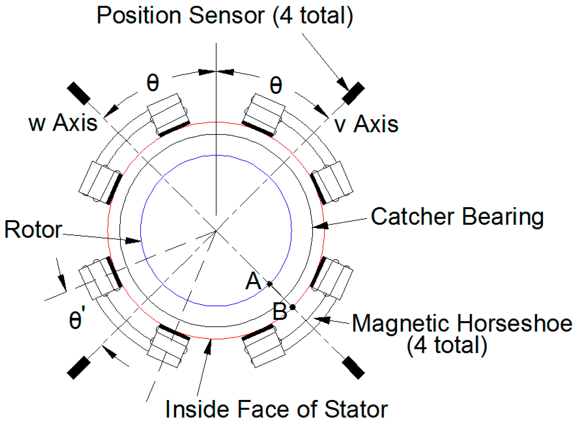
As shown in Figure 3, the geometric configuration of the AMB used in this research is comprised of two sets of opposing horseshoe actuators rotated at 45° from the vertical. Each actuator centerline is at an angle of θ′ (22.5°) with respect to each horseshoe centerline. Air gap, g, between the inner stator and outer rotor surface (Line AB in Figure 3), is a function of rotor position, xv, and is the rotor displacement along the v axis (μm). Similarly, xw is the rotor displacement along the w axis (μm).
As the controller receives set points xv, xw and biases iv,bias, iw,bias, current injection occurs at the top and bottom actuators, providing signal perturbation. The PID controller receives a feedback error signal by subtracting the desired set point (in volts) from the position sensor voltage.
2.4. Bearing Rotor Space Geometry
In order to establish rotor position with respect to the bearing stator, a geometric coordinate system is defined consisting of radial lines every 22.5° and circumferential grid lines every 25 μm. The origin of the system, which corresponds to the center of the catcher bearing, along with geometric axes and coordinates (xv,geo and xw,geo) are shown in Figure 4 for Quadrant 1. The horizontal axis corresponds to the geometric v axis, and the vertical axis corresponds to the geometric w axis, which in reality are oriented 45 degrees with respect to the vertical. Rotor Quadrants 2, 3 and 4 are partitioned similarly for a total of 65 geometric coordinates.
The actual rotor space is not circular as suggested by Figure 4, but consists of a thin annulus bounded by the stator and rotor. As the rotor moves radially from the geometric origin, the air gap decreases in the direction of rotor motion and increases in the opposite direction.
The magnetic field is assumed to be uniform between stator and rotor surfaces. In reality, the magnetic field may experience fringing and leakage due the rotor’s close proximity to the stator. These effects reduce the ability of the actuator to levitate loads due to a decrease in flux density near the edge of the pole face.
Ideally, the initial air gap, go, is assumed to be equal to 762 µm, but due to manufacturing tolerances, rotor-stator misalignment, and environment conditions, go may vary from this value. It is also assumed that position sensor alignment coincides with the centerline of each magnetic horseshoe. Any deviation from these ideal conditions reduces the positional accuracy needed to calculate bearing reaction values.
2.5. Reaction Measurement Using Geometric Coordinates and Geometric Set Points
To demonstrate the value of the proposed method, the force model described by Equation (1) was applied to a static rotor of known mass intentionally placed in several locations within the AMB working space by PID control. Controller-reported geometric coordinates were used to provide set points for the AMB while the bias current remained set to 1.5 A for all cases. The resulting currents in the v and w axis actuators were recorded for each location. The force model described by Equation (1) was then used to predict the bearing reaction force associated with the set point and resulting actuator currents for each scenario. The transducer measurement of load (19.75 N) does not change between bias perturbation or different set point scenarios, However,, some variation in the reaction force predicted by the model may be observed due to resolution of the current measurement.
To illustrate this approach, consider Station 11 (Figure 4), which has polar coordinates (50 μm, 45°) and corresponding v and w geometric coordinates of:
Here, r is the radial distance from the geometric origin and θ is measured counter clockwise from the positive geometric v axis. When the rotor set point was set to the controller-reported geometric coordinates of xv (35.36 µm) and xw (35.36 µm) and the bias current was set to 1.5 A, the control system responded with the actuator currents shown in Table 2.
Applying these geometric coordinate set points and measured actuator currents to Equation (1) results in the predicted bearing reaction force shown in the rightmost column of Table 2 (22.28 N). Current bias perturbation is not applied at this stage to demonstrate force measurements results without using the effective gap. The k parameter in Equation (1) is obtained from the bearing manufactures’ specifications (A, N) and the expected material physical constants (µo, b). The process of moving the rotor to a location specified by controller-reported geometric coordinates and observing the associated actuator currents was repeated for several locations within the AMB working space. The force model described by Equation (1) was applied to each case to predict bearing reaction force. The results are shown for each case in Table 3. Notice that xv and xw coordinate values shown in Columns 5 and 6 of Table 3 are the same as corresponding set point coordinates shown in Columns 7 and 8. This is done to illustrate that no set point coordinate transformation has yet occurred.
It can be seen that the average of the model predictions is 22.02 N, which differs from the transducer-based measurement by 11.6%. The percent difference (7.4%–16.2%) between the prediction of a model based on controller-reported geometric coordinates and transducer measurements observed in Table 3 lies near the middle of the range demonstrated by Prins [3] under similar circumstances (3%–22%) and is considered relatively large.
2.6. Transformation Equations
The method described in this paper accounts for misalignment effects previously noted by introducing an “effective” coordinate system that is rotated, scaled and displaced relative to the geometric coordinate system employed by the control system. Application of effective coordinates in the force model, Equation (1), results in improved prediction of bearing reaction force when compared to use of controller-reported geometric coordinates in the same model. The remapping of controller-based geometric coordinates to effective coordinates is realized by a coordinate transformation. In order to realize the coordinate transformation, rotation, scale and displacement parameters must be determined experimentally. Determination of the transformation parameters requires several applications of the multi-point method, but utilizes only existing AMB components since input variables into the force model consist of only (1) the gap between stator and rotor and (2) actuator current.
2.7. Rotational Transformation
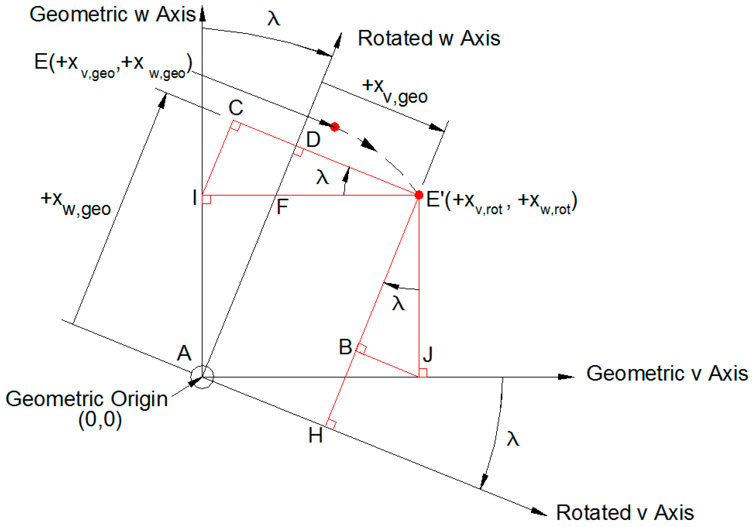
Rotational transformation involves orienting geometric v and w axes through an angle λ to align each along corresponding effective axes. In Figure 5, Point A is at the geometric origin (0, 0). Point E (xv,geo, xw,geo) represents a typical coordinate in the first rotor space quadrant rotated to the final position E′ (xv,rot, xw,rot). Points H and D are perpendicular projections of Point E′ onto the rotated v and w rotated axes, respectively. Points B, C, F, J and I are additional points used to derive expressions for xv,rot and xw,rot [3].
As shown in [3], resulting expressions for xv,rot and xw,rot as functions of xv,geo, xw,geo and λ are:
It is determined experimentally that different amounts of rotation result for the v and w directions, indicating that a true mapping of the rotor magnetic field results in a set of non-perpendicular axes. Due to the small differences in λv and λw, a mean value (λ) is used in final empirical transformation equations.
2.8. Scale and Displacement Transformation
Scale transformation involves scaling each axis to account for observed shortening (sv or sw < 1) or lengthening (sv or sw > 1) due to variations in the AMB magnetic field. Scale parameters sv and sw are determined from the slope of linear regression plots of geometric vs. effective coordinates. Scaling is required for both axes and varies as a function of the distance from the effective center, but due to the small variations observed, average values of sv and sw are used in final transformation equations.
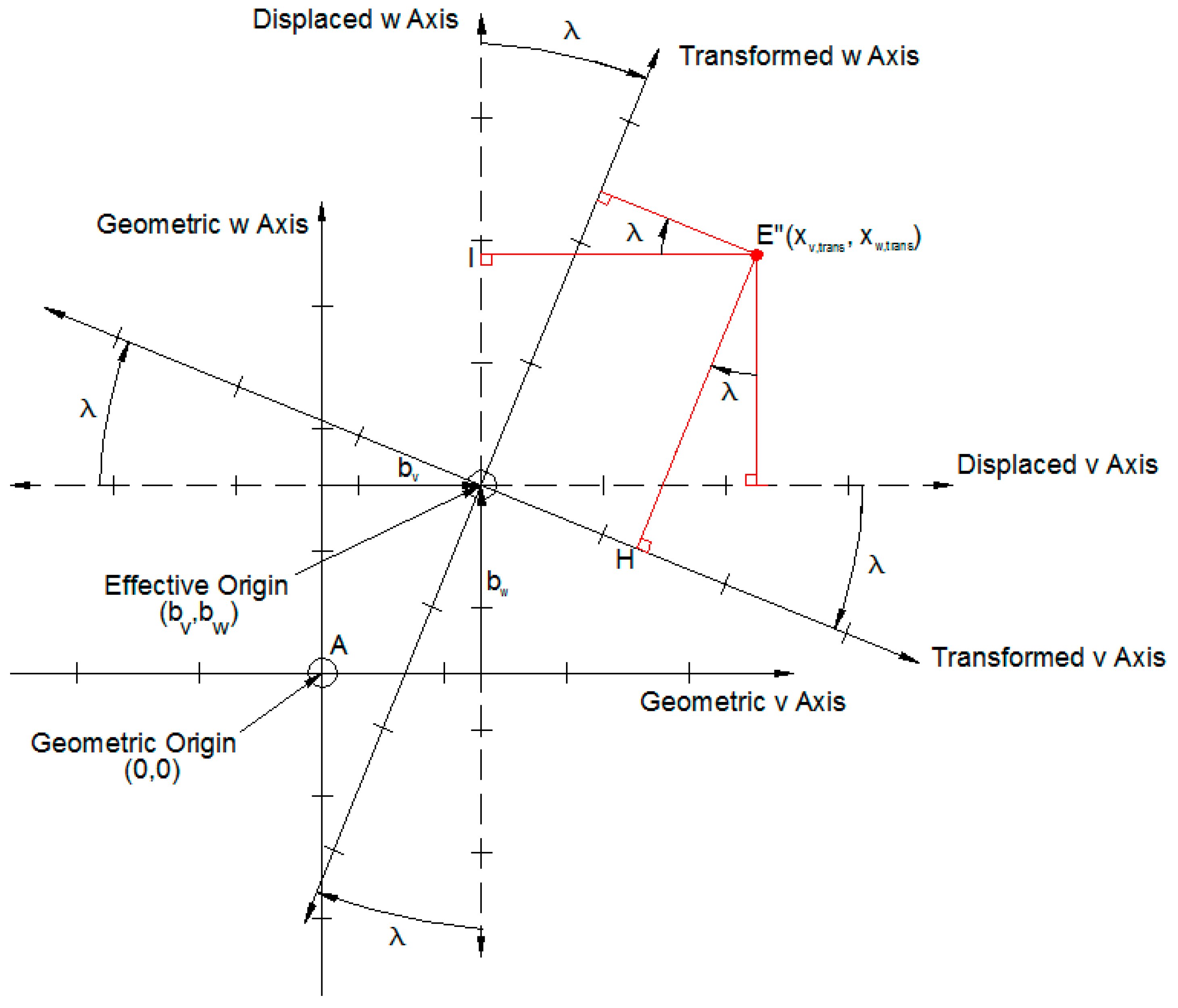
Displacement transformation results in a shift of coordinates a distance bv in the v direction and bw in the w direction, as shown in Figure 6, where Point E″ represents the final transformed coordinate location. Namely:
Equations (14) and (16) are functions of geometric coordinates and transformation parameters. As is shown in [3], expressions for xv,rot and xw,rot are the same for all rotor space coordinates. Therefore, Equations (14) and (16) may be applied at any location in the bearing’s operational space to obtain transformed coordinates.
3. Results
3.1. Locating the Effective Origin
In order to obtain empirical transformation equations, coordinates within the rotor space are selected as controller set points. Consider geometric coordinate (50, 50) μm, which produces the output currents shown in Table 4.
Using currents for a bias of 1.5 A and Equation (1), the total reaction is:
R = (48.55 N + 13.98 N) cos 45° = 44.22 N
This reaction is significantly in error when compared to the transducer value of 19.75 N. To quantify the error in terms of controller set points, parameter εn is introduced and defined as:
For this first iteration, n = 1. From Equation (8), xv,1 = 12.98 μm, xw,1 = 56.06 μm, and effective origin coordinates are xv,eff = 0, xw,eff = 0. Error is thus equal to:
Parameter εn tends to decrease as coordinates returned from successive iterations approach the effective origin. Set points for the next iteration are established by subtracting coordinates returned from iteration n from set points for iteration n−1:
xv,setpt,n = xv,setpt,n−1 − xv,n−1
Applying Equation (20), v and w axis set points for the second iteration (n = 2) are:
xv,setpt,2 = 50.00 − 12.98 = 37.02 µm
xw,setpt,2 = 50.00 − 56.08 = −6.08 µm
These new set points are supplied to the AMB controller; the system is again interrogated, and MPM coordinates (29.73, 2.94) μm result via Equation (8). The error for the second iteration becomes:
Table 5 shows the results of repeating the procedure for multiple iterations. The final error between coordinates (−0.92, −0.67) μm and effective origin (0, 0) μm is 1.14 μm, which is within 1% of the operational space of the rotor (±1.44 μm); therefore, the procedure is not repeated.
Figure 7 illustrates the relationship between coordinates returned from each iteration (shown as X in Figure 7) and the geometric coordinate system. The exploded view shows coordinates returned from Iterations 2–19. Set Point 19 lies within 1.44 μm of the effective origin as indicated by the smaller circle surrounding the coordinate. All coordinates shown in Figure 7 are with respect to the geometric origin.
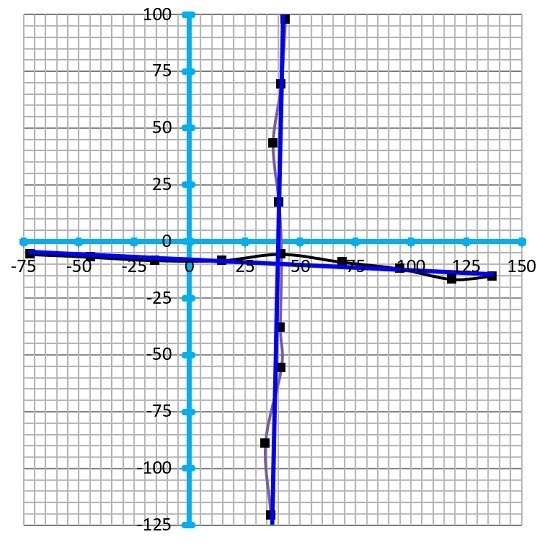
Figure 8 is a plot of iteration number vs. controller set points and MPM coordinates for the v axis; similar results occur for the w axis. Error parameter εn may be thought of as the magnitude of a vector equal to the MPM coordinate to effective coordinate distance for iteration n. Applying the error vector in this manner allows for the adjustment of both v and w set points simultaneously.
Set points returned from the final MPM iteration locate the rotor at the effective origin and represent its position with respect to the geometric origin. In short:
xv,setpt,final = 41.49 µm
xw,setpt,final = −5.57 µm
It can be seen in Figure 8 that the error initially tends toward the effective origin. However, if iterations are continued, excursions away from the effective origin do occur. These excursions remain within a noise band that demonstrates the limitations of the method for the system described herein. The method exhibits robustness in that the method continues to hunt for the origin in reaction to erroneous placements. The expected source of our limitations with respect to locating the effective origin is the current measurement uncertainty, which is beyond the scope of this paper.
3.2. Effective Coordinate Axes
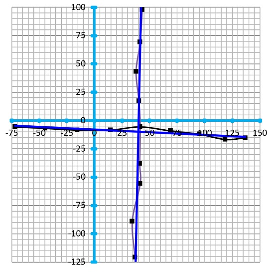
With the effective origin established, the procedure is repeated to determine v and w effective coordinate axes by moving to different set points to map out the rotor-stator gap area of interest. For example, the location of effective coordinate (25, 0) μm is determined to occur at xv = 69.19 µm and xw = −9.11 µm. Initial set points are established in this case by adding 25 μm to 41.49 μm for the v coordinate and 0 μm to −5.57 µm for the w coordinate. Using Equation (18), the error for the third iteration is:
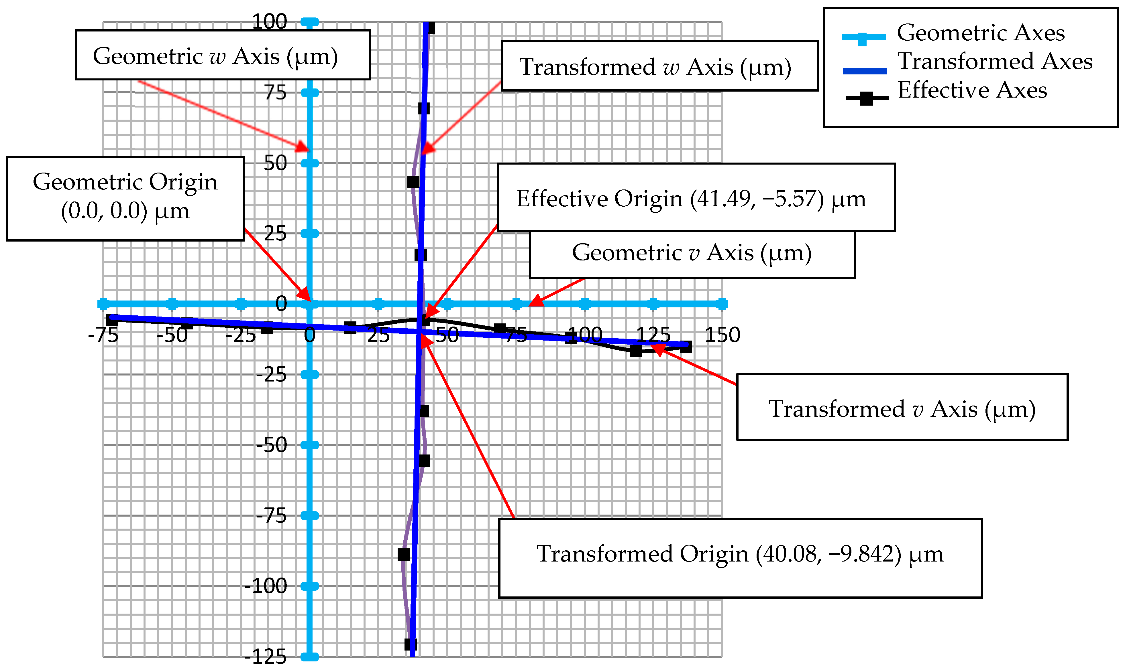
Since ε3 is within 1.44 μm, set points 69.19 μm and −9.11 μm represent the location of this effective coordinate with respect to the geometric origin. Performing similar computations, additional coordinates along the v and w axes result as shown as solid squares in Figure 9.
4. Empirical Transformation Equations
After establishing the effective coordinate system, numerical values for displacement, rotational and scale transformation parameters may be determined. Rotation parameters are found from the slope of linear regression curves for each effective axis shown in Figure 9. For the v axis (R2 = 0.71):
y = −0.04640x − 7.982
λv = tan−1 (−0.0464) = −2.657° (cw)
For the w axis (R2 = 1.00):
y = 45.89x − 1849
λw = tan−1 (45.893) − 90 = −1.2483° (cw)
An average absolute value of λ equal to 1.953° (cw), where cw indicates “clockwise”, is used in final transformation equations due to small variations observed for λv and λw.
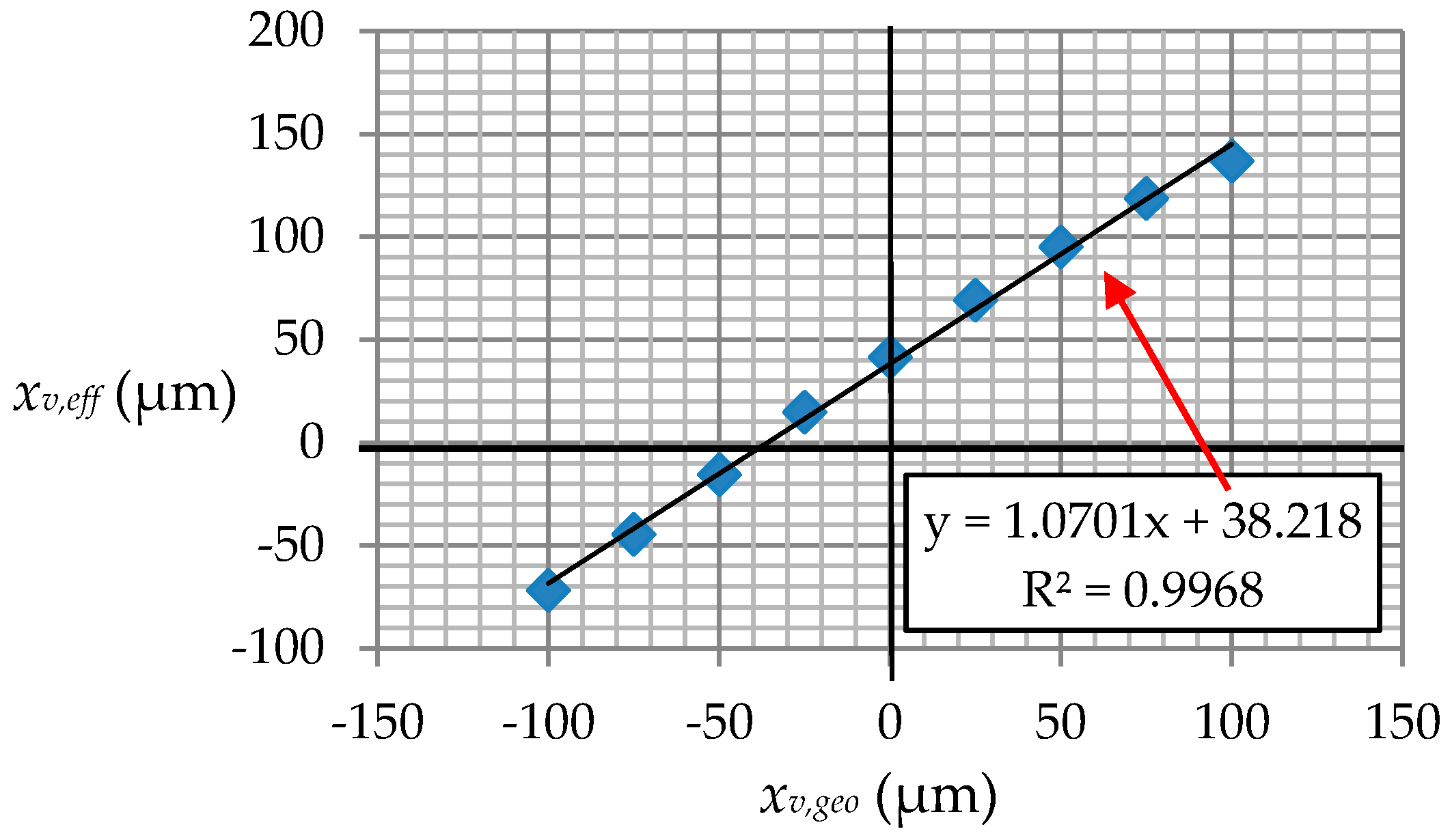
Scale parameters sv and sw are found by plotting geometric coordinates vs. effective coordinates for each rotor axis. The slope of the straight-line yields the scale factor for each axis [11]. Figure 10 shows the plot xv,geo vs. xv,eff, along with information on the linear regression fit. Similar results may be shown for the w axes.
From the slopes of the respective regression curves, sv is established to be 1.0701, and sw is 1.0698. Rotation, scale and displacement parameters may now be inserted into Equations (14) and (16) to obtain final empirical transformation equations. For the v axis:
xv,trans = (xv,geo cos 1.953° + xw,geo sin 1.953°) 1.0701 + 40.078
xv,trans = 1.06947 xv,geo + 0.036468 xw,geo + 40.078
Similarly for the w axis:
xw,trans = −0.036458 xv,geo + 1.06868 xw,geo − 9.8416
Reaction Measurement using Corrected Set Points
With empirical transformation equations completed, v and w geometric coordinates from any location in the rotor space may be substituted into Equations (32) and (33) to obtain correct set points that indicate the effective origin. To illustrate this, the static outboard bearing reaction in a non-rotating scenario is calculated by placing the rotor at the effective origin and measuring output currents as shown in Table 6.
Using output currents from Table 6 for a 1.5-A bias and geometric coordinates (0.0, 0.0) µm in Equation (1) results in:
Fv = 13.53 N
Fw = 13.74 N
R = cos 45° (13.53 N + 13.74 N) = 19.28 N
For biases 1.3 A and 1.7 A, R = 19.37 N and 19.25 N, respectively, for an average of 19.3 N.
Additional static reaction measurements are taken at 16 other locations throughout the rotor space, as shown in Table 7. It can be seen that application of effective coordinates to the force prediction model reduces the average difference between model prediction and transducer measurement from 11.6% down to 2.77%, with a range of error from −4.28% to 5.86%.
5. Conclusions
This study demonstrates the use of a non-invasive, in situ method to determine an effective coordinate system for an AMB. An empirical process that makes use of bias current perturbation (multi-point method, MPM) is employed to develop a coordinate transformation between controller-reported geometric coordinates and effective coordinates. The use of effective coordinates in a static bearing reaction force model is shown to reduce average differences between predicted force values and transducer measurements of forces from 11.6%, using expected gap values from manufacturer set-point data, down to 2.77%, using effective gap values as determined by the application of the error vector for magnetic axis correction presented here that was developed through an extension of the application of the MPM system identification approach.
Author Contributions
Robert Prins provided assistance during initial experimental design and assisted in writing the paper. Mary Kasarda served as the major research advisor and assisted in writing the paper. Dewey Spangler, Jr. performed the experiments, analyzed the data and assisted in writing the paper.
Conflicts of Interest
The authors declare no conflict of interest.
Nomenclature
| A | area of two pole faces (2 faces per horseshoe) = 2.992 × 10⁻⁴ m2 |
| Fmagnetic | force due to magnetic source (N) |
| Li | flux path through rotor and stator (0.045 m) [2] |
| N | number of wire turns for two actuator coils (two coils per horseshoe) = 248 |
| b | Li/μr = manufacturer’s equivalent air gap based on magnetic reluctance of magnetic material (15.0 × 10⁻⁶ m) |
| ε | parameter to quantify the error between the bearing force obtained from force transducers and the force obtained from an MPM iteration |
| go | air gap between rotor and magnetic horseshoe when rotor and stator geometric centers are concentric |
| gtop | air gap between top of rotor and inside face or stator |
| gbottom | air gap between bottom of rotor and inside face or stator |
| i | total current in single magnetic horseshoe |
| itop | total current at top horseshoe |
| ibottom | total current at bottom horseshoe |
| λ | angle between the geometric v and w axes and the transformed v and w axes, respectively |
| R | Magnitude of the vector resultant of the magnetic forces along the v and w axes |
| θ | angle between the vertical axis and the v or w magnetic axes |
| θ′ | angle between the v or w magnetic axes and the axes of the position sensor |
| xv,n | v axis coordinate returned from MPM iteration n |
| xv,eff | desired v axis effective coordinate |
| xw,n | w axis coordinate returned from MPM iteration n |
| xw,eff | desired w axis effective coordinate |
| xv,geo, xw,geo | measured from the geometric center of the bearing located at the intersection of v and w sensor axes. Geometric coordinates are based on the assumption that the magnetic field is in perfect alignment with the rotor geometric center, magnetic axes and positional sensor axes. |
References
- Marshall, J.; Kasarda, M.; Imlach, J. A Multi-Point Measurement Technique for the Enhancement of Force Measurement with Active Magnetic Bearings. ASME J. Eng. Gas Turbine Power 2003, 125, 90–94. [Google Scholar] [CrossRef]
- Prins, R. System Identification and Calibration Techniques for Force Measurement in Active Magnetic Bearing. Ph.D. Thesis, Virginia Tech., Blacksburg, VA, USA, 2005, Section 1.1 (unpublished). [Google Scholar]
- Prins, R.J.; Kasarda, M.E.F.; Bates, S.C. A System Identification Technique Using Bias Current Perturbation for Determining Effective Rotor Origin of Active Magnetic Bearings. ASME J. Vib. Acoust. 2007, 129, 317–322. [Google Scholar] [CrossRef]
- Kasarda, M. An Overview of Active Magnetic Bearing Technology and Applications. Shock Vib. Dig. 2000, 32, 91–99. [Google Scholar] [CrossRef]
- Gahler, C.; Forch, P. A Precise Magnetic Bearing Exciter for Rotordynamic Experiments. In Proceedings of the Fourth International Symposium on Magnetic Bearings, Zurich, Switzerland, 23–26 August 1994. [Google Scholar]
- Rantatalo, M.; Aidanpaa, J.; Goransson, B.; Norman, P. Milling Machine Spindle Analysis Using FEM and Non-Contact Spindle Excitation and Response Measurement. Int. J. Mach. Tools Manuf. 2007, 47, 1034–1045. [Google Scholar] [CrossRef]
- Auchet, S.; Chevrier, P.; Lacour, M.; Lipinski, P. A New Method of Cutting Force Measurement Based on Command Voltages of Active Electro-Magnetic Bearings. Int. J. Mach. Tools Manuf. 2004, 44, 1441–1449. [Google Scholar] [CrossRef]
- Aenis, M.; Knopf, E.; Nordmann, R. Active Magnetic Bearings for the Identification and Fault Diagnosis in Turbomachinery. Mechatronics 2002, 12, 1011–1021. [Google Scholar] [CrossRef]
- Hussien, A.A.; Yamada, S.; Iwahara, M.; Okada, T.; Ohji, T. Application of the Repulsive-Type Magnetic Bearing for Manufacturing Micromass Measurement Balance Equipment. IEEE Trans. Magn. 2005, 41, 3802–3804. [Google Scholar] [CrossRef]
- Plonus, M.A. Applied Electromagnetics; Section 10.7; McGraw-Hill: New York, NY, USA, 1978. [Google Scholar]
- Spangler, D. Application of a Bias Current Perturbation Method for Determining Effective Gaps in Magnetic Bearings Utilizing an Error Vector Concept; Mechanical Engineering Master of Engineering Final Report; Virginia Tech: Blacksburg, VA, USA, 2011. [Google Scholar]
- MBRotor Research Test Stand (no. 893-0005-001-05/98). In Hardware User’s Guide, version 1.0; Section 2.4; Revolve Magnetic Bearings Inc.: Calgary, AB, Canada, 1998.
Figure 1.
Equilibrium of a magnetically-suspended object.
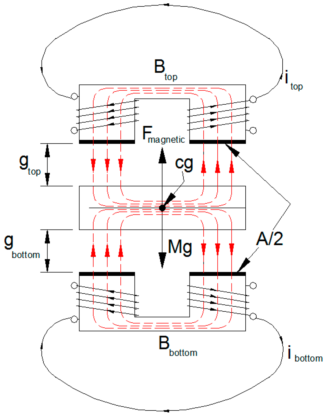
Figure 2.
Experimental rotor test stand configuration (photo: [2]).
Figure 2.
Experimental rotor test stand configuration (photo: [2]).

Figure 3.
Active Magnetic Bearing (AMB) configuration.

Figure 4.
Geometric coordinates for rotor space Quadrant 1.
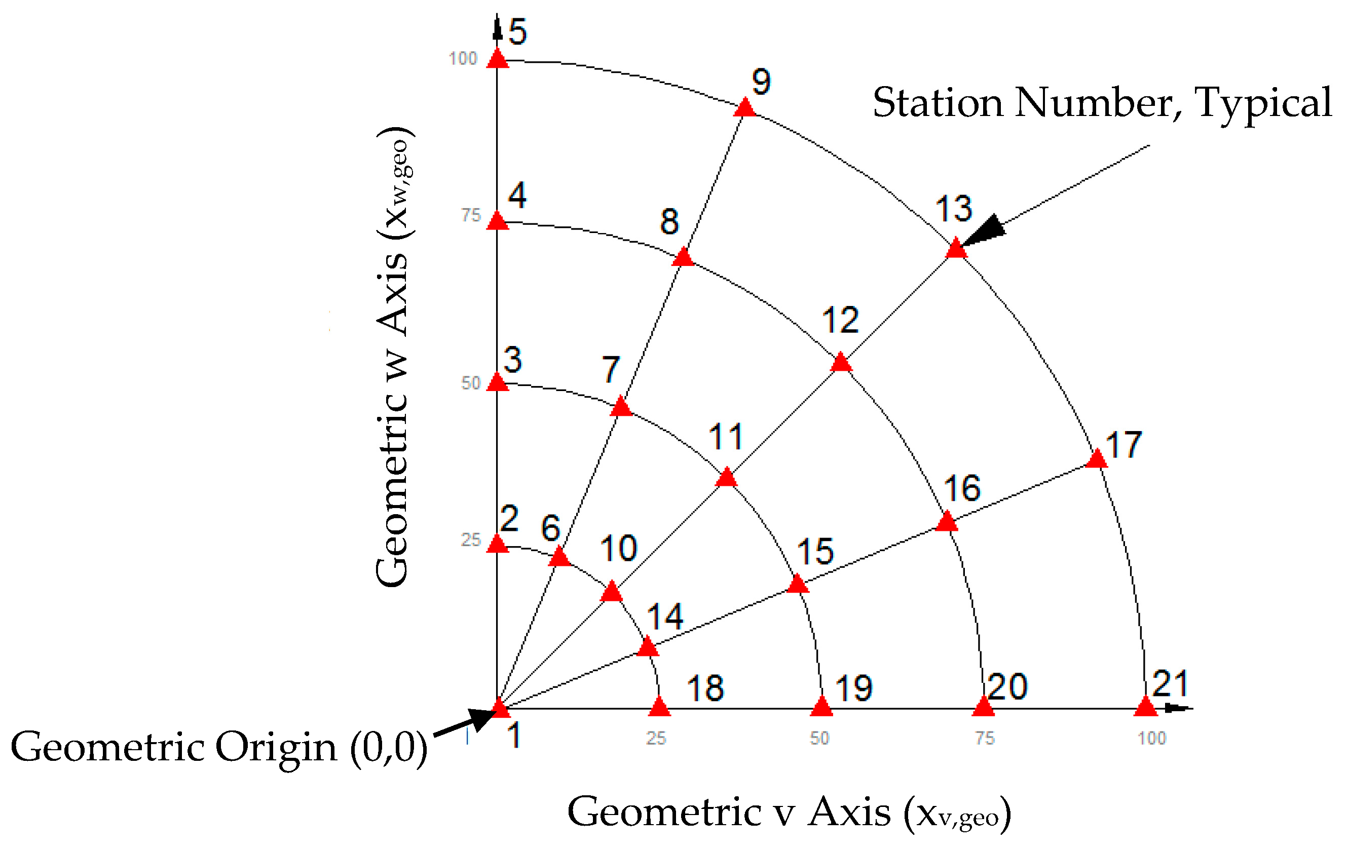
Figure 5.
Rotation of geometric coordinate axes in Quadrant 1.

Figure 6.
Transformed coordinates with respect to geometric origin.

Figure 7.
Spatial relationship between geometric and effective origins. All values shown are in microns (µm).
Figure 7.
Spatial relationship between geometric and effective origins. All values shown are in microns (µm).
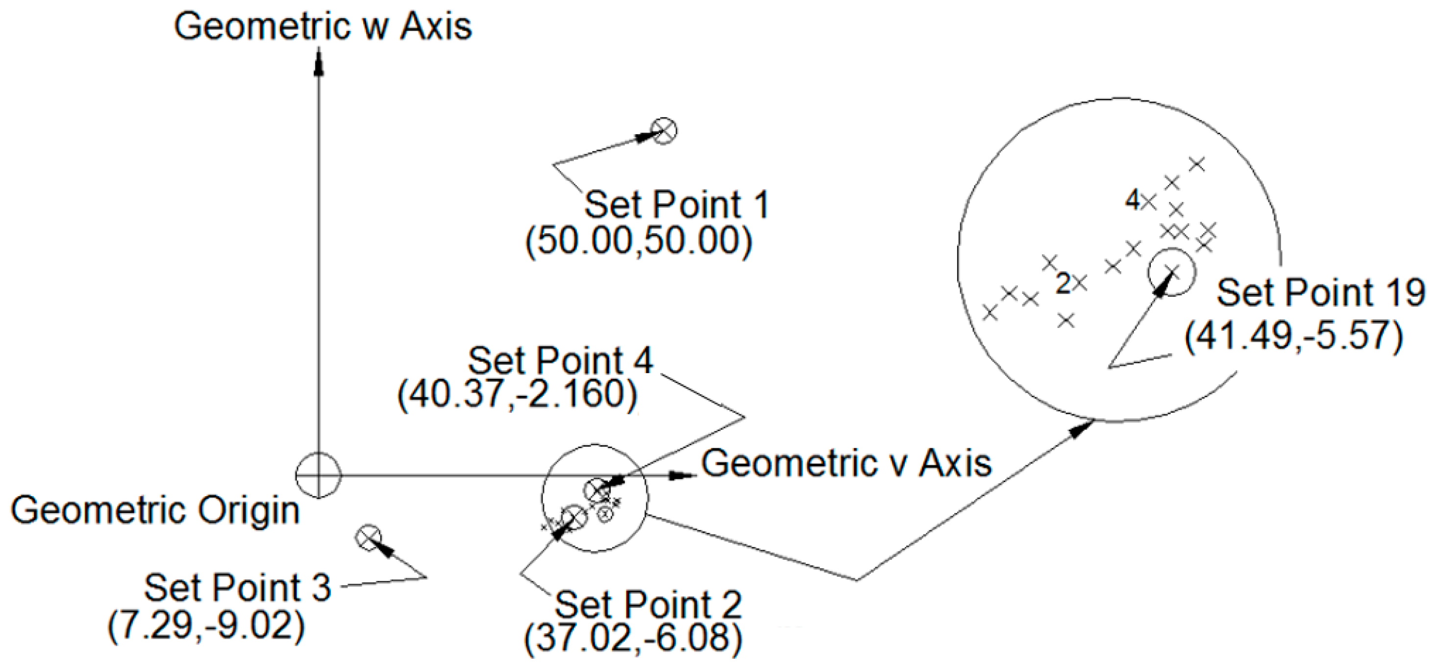
Figure 8.
Iteration vs. set point and v axes MPM coordinate.
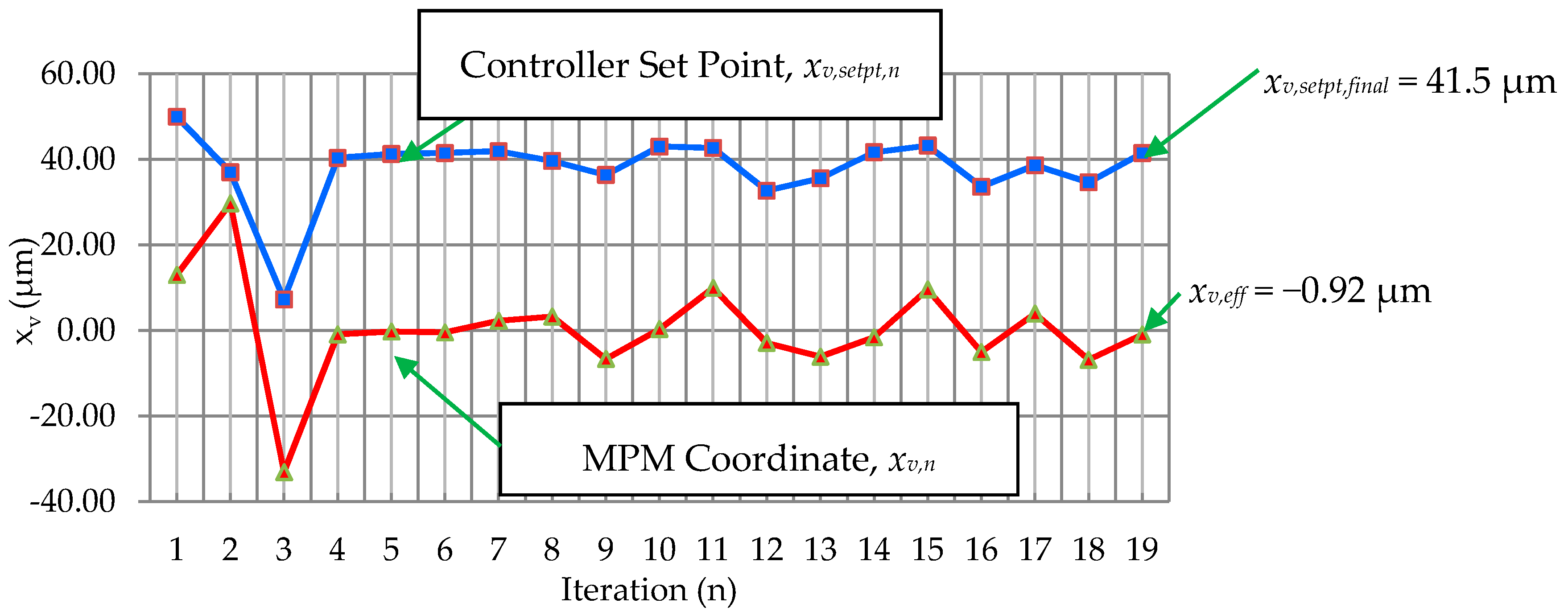
Figure 9.
Relationship between geometric, transformed and effective origins.

Figure 10.
Geometric vs. effective coordinates for the v axis.

Table 1.
Transducer reaction measurement.
| Run | Sum of AMB Outboard Reaction (N) |
|---|---|
| 1 | 19.4 |
| 2 | 19.5 |
| 3 | 19.7 |
| 4 | 19.3 |
| 5 | 20.6 |
| 6 | 20.1 |
| 7 | 19.5 |
| 8 | 19.8 |
| 9 | 19.8 |
| 10 | 19.8 |
| Average | 19.8 |
Table 2.
Output current and bearing reaction at set point (35.36, 35.36) μm.
| Bias Current (Amp) | iv,top | iw,top | iv,bottom | iw,bottom | Bearing Reaction R (N) |
|---|---|---|---|---|---|
| 1.5 | 1.768 | 1.670 | 1.228 | 1.305 | 22.28 |
Table 3.
Reaction measurement using geometric coordinates and geometric current set points (bias current = 1.5 Amp).
Table 3.
Reaction measurement using geometric coordinates and geometric current set points (bias current = 1.5 Amp).
| Station | Quadrant | Polar Coordinate R (μm) | Polar Coordinate Θ (°) | xv (μm) | xw (μm) | xv,setpoint (μm) | xw,setpoint (μm) | Reaction R (N) | Percent Difference |
|---|---|---|---|---|---|---|---|---|---|
| 1-origin | 1 | 0 | 90 | 0.00 | 0.00 | 0.00 | 0.00 | 22.02 | 11.5 |
| 3-positive (pos) w axis | 1 | 50 | 90 | 0.00 | 50 | 0.00 | 50 | 22.51 | 14 |
| 5-pos w axis | 1 | 100 | 90 | 0.00 | 100 | 0.00 | 100 | 22.95 | 16.2 |
| 11 (from Table 2) | 1 | 50 | 45 | 35.36 | 35.36 | 35.36 | 35.36 | 22.28 | 12.8 |
| 13 | 1 | 100 | 45 | 70.71 | 70.71 | 70.71 | 70.71 | 22.46 | 13.7 |
| 19-pos v axis | 1 | 50 | 0 | 50.0 | 0.00 | 50.0 | 0.00 | 22.06 | 11.7 |
| 21-pos v axis | 1 | 100 | 0 | 100 | 0.00 | 100 | 0.00 | 22.28 | 12.8 |
| 51-negative (neg) v axis | 2 | 50 | 180 | −50.0 | 0.00 | −50.0 | 0.00 | 21.84 | 10.6 |
| 53-neg v axis | 2 | 100 | 180 | −100 | 0.00 | −100 | 0.00 | 22.37 | 13.3 |
| 59 | 2 | 50 | 135 | −35.36 | 35.36 | −35.36 | 35.36 | 22.24 | 12.6 |
| 61 | 2 | 100 | 135 | −70.71 | 70.71 | −70.71 | 70.71 | 22.60 | 14.4 |
| 35-neg w axis | 3 | 50 | 270 | 0.00 | −50 | 0.00 | −50 | 21.44 | 8.56 |
| 37-neg w axis | 3 | 100 | 270 | 0.00 | −100 | 0.00 | −100 | 21.22 | 7.43 |
| 43 | 3 | 50 | 225 | −35.36 | −35.36 | −35.36 | −35.36 | 21.75 | 10.1 |
| 45 | 3 | 100 | 225 | −70.71 | −70.71 | −70.71 | −70.71 | 21.35 | 8.11 |
| 27 | 4 | 50 | 315 | 35.36 | −35.36 | 35.36 | −35.36 | 21.66 | 9.68 |
| 29 | 4 | 100 | 315 | 70.71 | −70.71 | 70.71 | −70.71 | 21.57 | 9.23 |
| Average | 22.02 | 11.6% |
Table 4.
Output currents at set point (50, 50) μm.
| Bias Current (Amp) | iv,top | iw,top | iv,bottom | iw,bottom |
|---|---|---|---|---|
| 1.3 | 1.579 | 1.500 | 1.015 | 1.086 |
| 1.5 | 1.738 | 1.646 | 1.259 | 1.331 |
| 1.7 | 1.904 | 1.797 | 1.495 | 1.569 |
Table 5.
Application of Multi-Point Method (MPM) to determine the location of effective origin at (0, 0) μm.
Table 5.
Application of Multi-Point Method (MPM) to determine the location of effective origin at (0, 0) μm.
| Iteration (n) | xv,setpt,n (μm) | xw,setpt,n (μm) | xv,n Returned from MPM Iteration, n (μm) | xw,n Returned from MPM Iteration, n (μm) | εn |
|---|---|---|---|---|---|
| 1 | 50.00 | 50.00 | 12.98 | 56.08 | 57.54 |
| 2 | 37.02 | −6.08 | 29.73 | 2.94 | 29.88 |
| 3 | 7.29 | −9.02 | −33.08 | −6.86 | 33.78 |
| 4 | 40.37 | −2.16 | −0.9 | 1.39 | 1.66 |
| 5 | 41.27 | −3.55 | −0.23 | −2.32 | 2.33 |
| 6 | 41.5 | −1.23 | −0.43 | 2.37 | 2.41 |
| 7 | 41.93 | −3.6 | 2.28 | 0.81 | 2.42 |
| 8 | 39.65 | −4.41 | 3.27 | 3.49 | 4.78 |
| 9 | 36.38 | −7.9 | −6.64 | −3.66 | 7.58 |
| 10 | 43.02 | −4.24 | 0.34 | −4.57 | 4.58 |
| 11 | 42.68 | 0.33 | 9.98 | 7.84 | 12.69 |
| 12 | 32.7 | −7.51 | −2.89 | −2.39 | 3.75 |
| 13 | 35.59 | −5.12 | −6.09 | −2.6 | 6.62 |
| 14 | 41.68 | −2.52 | −1.57 | 1.01 | 1.87 |
| 15 | 43.25 | −3.53 | 9.62 | 3.04 | 10.09 |
| 16 | 33.63 | −6.57 | −5 | −1.28 | 5.16 |
| 17 | 38.63 | −5.29 | 3.97 | 1.56 | 4.27 |
| 18 | 34.66 | −6.85 | −6.83 | −1.28 | 6.95 |
| 19 | 41.49 | −5.57 | −0.92 | −0.67 | 1.14 |
Table 6.
Output currents and bearing reactions at set point (41.49, −5.57) μm.
| Bias Current (Amp) | iv,top | iw,top | iv,bottom | iw,bottom | Bearing Reaction R (N) |
|---|---|---|---|---|---|
| 1.3 | 1.590 | 1.588 | 1.008 | 0.998 | 19.37 |
| 1.5 | 1.751 | 1.744 | 1.251 | 1.232 | 19.28 |
| 1.7 | 1.923 | 1.909 | 1.482 | 1.458 | 19.25 |
Table 7.
Reaction measurement: geometric coordinates/transformed set points.
| Station | Quad. | xv (μm) | xw (μm) | xv,setpoint (μm) | xw,setpoint (μm) | Reaction R (N) | Percent Diff. |
|---|---|---|---|---|---|---|---|
| 1-origin | 1 | 0.00 | 0.00 | 44.11 | −6.92 | 19.26 | −2.48 |
| 3-pos w axis | 1 | 0.00 | 50 | 46.59 | 46.51 | 19.13 | −3.15 |
| 5-pos w axis | 1 | 0.00 | 100 | 49.07 | 99.94 | 19.22 | −2.7 |
| 11 | 1 | 35.36 | 35.36 | 83.69 | 30.04 | 18.90 | −4.28 |
| 13 | 1 | 70.71 | 70.71 | 123.27 | 66.99 | 19.04 | −3.6 |
| 19-pos v axis | 1 | 50.0 | 0.00 | 97.6 | −8.08 | 18.90 | −4.28 |
| 21-pos v axis | 1 | 100 | 0.00 | 151.1 | −9.25 | 20.91 | 5.86 |
| 51-neg v axis | 2 | −50.0 | 0.00 | −9.38 | −5.75 | 19.30 | −2.25 |
| 53-neg v axis | 2 | −100 | 0.00 | −62.87 | −4.59 | 19.75 | 0.00 |
| 59 | 2 | −35.36 | 35.36 | 8.04 | 31.69 | 19.17 | −2.93 |
| 61 | 2 | −70.71 | 70.71 | −28.03 | 70.29 | 19.70 | −0.23 |
| 35-neg w axis | 3 | 0.00 | −50 | 41.63 | −60.35 | 19.17 | −2.93 |
| 37-neg w axis | 3 | 0.00 | −100 | 39.15 | −113.78 | 19.17 | −2.93 |
| 43 | 3 | −35.36 | −35.36 | 4.53 | −43.88 | 19.48 | −1.35 |
| 45 | 3 | −70.71 | −70.71 | −35.05 | −80.83 | 19.53 | −1.13 |
| 27 | 4 | 35.36 | −35.36 | 80.18 | −45.52 | 19.13 | −3.15 |
| 29 | 4 | 70.71 | −70.71 | 116.25 | −84.13 | 18.99 | −3.83 |
| Average | 19.34 | −2.77% |
© 2017 by the authors. Licensee MDPI, Basel, Switzerland. This article is an open access article distributed under the terms and conditions of the Creative Commons Attribution (CC BY) license (http://creativecommons.org/licenses/by/4.0/).
Share and Cite
MDPI and ACS Style
Spangler, D.; Prins, R.; Kasarda, M. A System Identification Technique Using Bias Current Perturbation for the Determination of the Magnetic Axes of an Active Magnetic Bearing. Actuators 2017, 6, 13. https://doi.org/10.3390/act6020013
AMA Style
Spangler D, Prins R, Kasarda M. A System Identification Technique Using Bias Current Perturbation for the Determination of the Magnetic Axes of an Active Magnetic Bearing. Actuators. 2017; 6(2):13. https://doi.org/10.3390/act6020013
Chicago/Turabian StyleSpangler, Dewey, Robert Prins, and Mary Kasarda. 2017. "A System Identification Technique Using Bias Current Perturbation for the Determination of the Magnetic Axes of an Active Magnetic Bearing" Actuators 6, no. 2: 13. https://doi.org/10.3390/act6020013
Note that from the first issue of 2016, this journal uses article numbers instead of page numbers. See further details here.