
Power Split Based Dual Hemispherical Continuously Variable Transmission
by
Douwe Dresscher
1,*, 
Mark Naves
2,
Theo J. A. De Vries
1,
Martijn Buijze
3 and
Stefano Stramigioli
1 1
Robotics and Mechatronics Group, CTIT Institute, University of Twente, 7522 NB Enschede, The Netherlands
2
Precision Engineering Group, University of Twente, 7522 NB Enschede, The Netherlands
3
DEMCON, Institutenweg 25, 7521 PH Enschede, The Netherlands
*
Author to whom correspondence should be addressed.
Actuators 2017, 6(2), 15; https://doi.org/10.3390/act6020015
Submission received: 26 February 2017
/
Revised: 17 March 2017
/
Accepted: 29 March 2017
/
Published: 10 April 2017
(This article belongs to the Special Issue Variable Stiffness and Variable Impedance Actuators)
Abstract
:In this work, we present a new continuously variable transmission concept: the Dual-Hemi Continuously Variable Transmission (CVT). It is designed to have properties we believe are required to apply continuously variable transmissions in robotics to their full potential. These properties are a transformation range that includes both positive and negative ratios, back-drivability under all conditions, kinematically decoupled reconfiguration, high efficiency of the transmission, and a reconfiguration mechanism requiring little work for changing the transmission ratio. The design of the Dual-Hemi CVT and a prototype realisation are discussed in detail. We show that the Dual-Hemi CVT has the aforementioned desired properties. Experiments show that the efficiency of the CVT is above 90% for a large part of the range of operation of the CVT. Significant stiction in the transmission, combined with a relatively low bandwidth for changing the transmission ratio, may cause problems when applying the DH-CVT as part of an actuator in a control loop.
1. Introduction
A Continuously Variable Transmission (CVT) is a transmission that allows “shifting” of the transmission ratio over a continuous range. CVTs have been around for a while and many designs have been proposed (see, for example, [1,2,3]). In addition, some Variable Stiffness Actuators contain a form of infinitely or continuously variable transmissions (see, for example, [4,5,6,7]). Mechanical CVTs can be divided into four categories: Traction-based CVTs, Belt CVTs, Ratcheting CVTs and Variable lever-arm CVTs. In [1,3], an overview/review of several existing types of CVTs is given.
In this work, we propose a new traction-based CVT concept: the Dual-Hemi CVT. Traction based CVTs use a rolling frictional contact to transmit power. In many traction-based CVTs, the action that changes the transmission ratio has to push through the same frictional contact that is used to transmit power. Thus, changing the transmission ratio requires a large amount of work. There are some designs where this is not required, the most notable being [8,9]. In most traction-based CVTs, changing the transmission ratio is kinematically decoupled from the transmission itself, and energy can be transferred in both directions. However, most of these designs have a transmission ratio range that only spans a positive (or negative) range (also here, [8] is an exception). The transmission ratio range can be extended using the power-split principle [1,10], where a differential or a planetary gear is used to extend the range of ratios. This does introduce extra losses and possibly has consequences for the back-drivability [10].
Electric motors are frequently applied in robotics. Although they are versatile, they are also energy-inefficient in high-torque, low-velocity range that is typical in robotics ([11]): they are only very efficient in a narrow range of operation (namely: low torque, high velocity). Using a combination of an electric motor with a CVT and optionally a mechanical storage element (as for example described in [12,13,14]), the electric motor can operate in its high-efficiency region while the combination is able to provide the torques required by the application.
We believe that a CVT applied for this purpose should have at least the following properties:
- 1.
- To use the CVT for energy transfer both from the source to the load and vice versa, as well as the option not to transfer energy, for a wide range of output loads, the transmission range needs to include positive ratios, negative ratios and a zero or infinite ratio.
- 2.
- Building on point 1, the system needs to be back-drivable under all conditions.
- 3.
- For the actuation energy not to be delivered by the reconfiguration actuator, changing the transmission ratio needs to be kinematically decoupled from the transmission such that:
- (a)
- Changing the transmission ratio does not perform work on other parts of the system.
- (b)
- It is possible to change the transmission ratio when the system is loaded (non-zero forces on“Energy source” and “Load”).
In addition, to achieve a high level of energy efficiency, the CVT needs to be designed such that:
- 4.
- The transmission has a high efficiency.
- 5.
- Changing the transmission ratio requires little work.
The Dual-Hemi CVT is aimed to have these properties.
In Section 2, we give some background on the power-split principle. Section 3 and Section 4 cover the concept and important design details, respectively, of the Dual-Hemi CVT. The prototype realisation is discussed in Section 5 and Section 6 important properties of the prototype are presented. This is followed by a discussion and exploration on several design choices in Section 7. Section 8 concludes the work with the most important findings.
2. Power Split Based CVTs
The first requirement is a range of ratios including the positive ratios, negative ratios and a zero or infinite ratio.
When mechanical CVTs are considered, this spread in ratios including the positive and negative ratios inherently requires a transition region where input and output are unrelated (a zero or infinite ratio). For traction-based CVTs, this region typically requires a sliding contact, since rotational velocity of input and output are decoupled for this ratio. As an example, the CVT design given by Peshkin can be considered [8]. As this sliding contact in the transition region typically causes high levels of wear, friction and energy losses, such a system is impractical in many applications. In order to prevent the necessity of this unfavourable transition region, while obtaining a mechanical system with the required range of ratios, the power split principle can be used (see, for example [1]).
When applying this principle, care should be taken regarding the losses introduced by the extra gears and the effect that this may have on the reversibility [10].
3. Dual-Hemispherical CVT Concept Design
This section describes a new innovative concept for a continuously variable transmission, named “dual hemispherical CVT” (DH-CVT).
This concept exchanges power between input and output by a purely rolling contact of two spherical elements, resulting in a high running efficiency (property 4). Furthermore, the force required to adjust the transmission ratio does not have to break through a frictional contact or preload, enabling an energy-efficient change of transmission ratio (property 5).
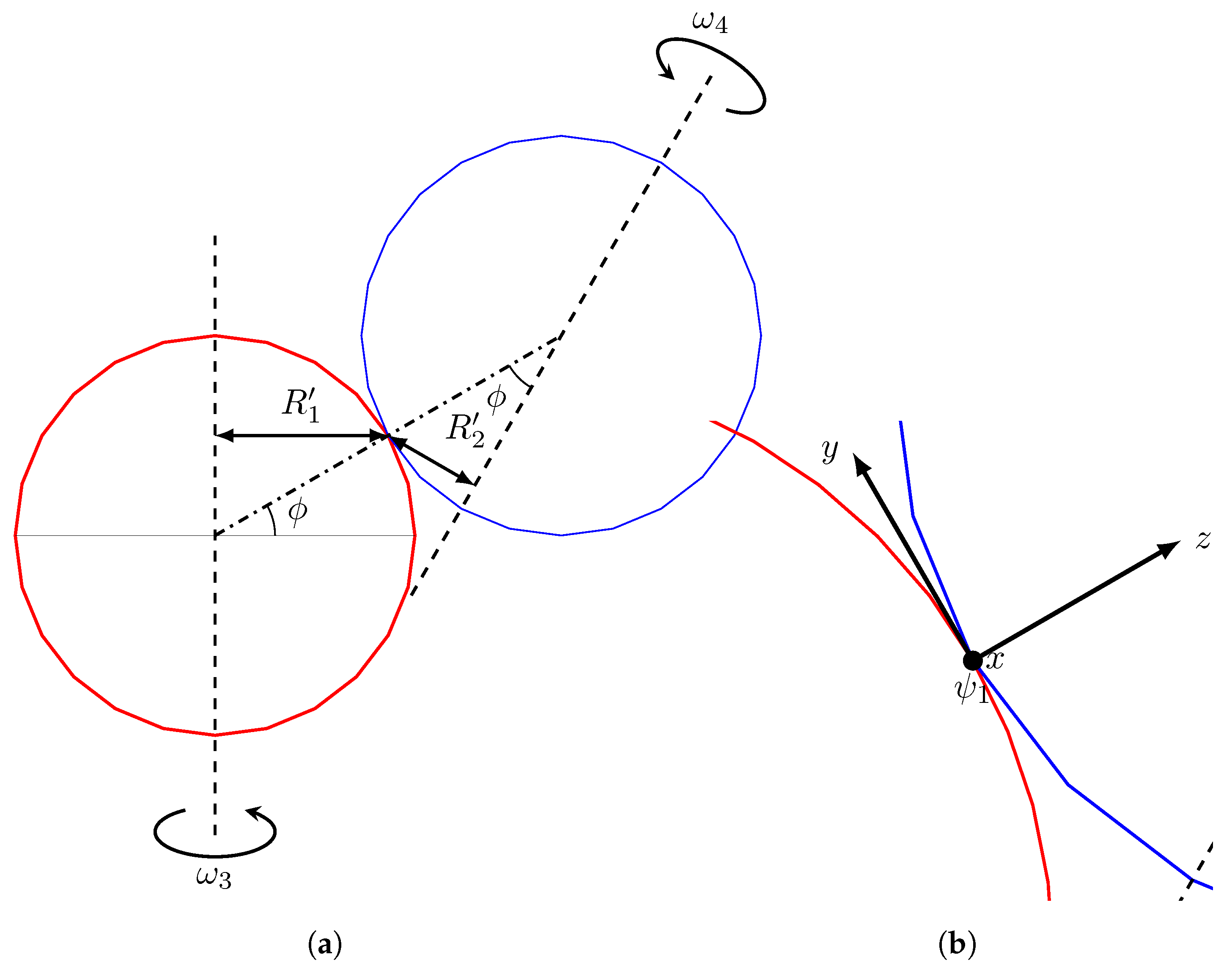
By changing the angle at which both spheres are aligned, the transmission ratio can be changed: the effective distance between the frictional contact and the axis of rotation of each sphere changes, resulting in a shift in transmission ratio. As the alignment can be changed by a pure rolling motion of both hemispherical elements, a change in transmission ratio can be realised with minimal adjustment force. To enable this pure rolling motion, the intermediate distance between the center of each friction wheel is equal to the sum of the radii of both friction wheels over the entire configuration range. A schematic overview of this concept is shown in Figure 1a, where the red spherical element is held in a stationary configuration, while the blue spherical element “rolls” over the red one in order to change the effective transmission ratio.
Changing the transmission ratio is kinematically decoupled from the transmission, as is shown in Figure 1b. In this image, changing the transmission ratio is a rotation around the x-axis while the transmission works by a translation along the x-axis. Due to this property, changing the transmission ratio does not directly change the state of the system and it is possible to change the transmission ratio when the system is loaded (property 3).
A comparison of the Dual-Hemi CVT with the most notable alternative CVT principles as described in [8,9] shows that they all use the the principle of changing an effective radius in a distinctively different way. In [8] a sphere is used, whose motion in constrained by several rollers. By the configuration of the rollers, the sphere is constrained to roll around an axis and by rotating two of the rollers, the constraints and thus the axis of rotation can be changed. Depending on the axis of rotation, different effective radii are created with respect to the two driving rollers—thereby changing the transmission ratio. In [9], the CVT is created by moving the ring gear over the conic planet gears such that the effective radius of the planets is changed—thereby changing the transmission ratio.
3.1. DH-CVT Transmission Ratio
The transmission ratio of the DH-CVT is determined by the contact angle between both hemispheres. This ratio is equal to the ratio between the effective radius and as illustrated in Figure 1a. This effective radius is defined by the distance between the axis of rotation and the contact point of each spherical element. The radius of each sphere is made equal to minimize local contact stress at the contact region [15] () and furthermore the spheres are configured such that at a configuration angle of 45 degrees, the transmission ratio between input and output equals one.
The resulting transmission ratio as function of the configuration angle is then given by the geometrical tangent of the configuration angle according to
If spherical friction wheels are considered, the configuration angle could theoretically be set over a range of 0 to radians, resulting in a range of transmission ratios from : see Figure 2.
However, as discussed in Section 2, a transmission ratio of at rad or 0 at rad, which decouples the output from the input, will result in a sliding contact between both friction wheels (input is fixed, output is free to rotate or vice versa). As this sliding contact will reduce efficiency and create high levels of wear, this configuration should be avoided. A configuration angle of with the corresponding transmission ratio of is considered, where the allowable range of configuration angles should be sufficiently distant from 0 and rad in order to prevent slip. This will be discussed in more depth in Section 4.2.
3.2. PS-CVT Transmission Ratio
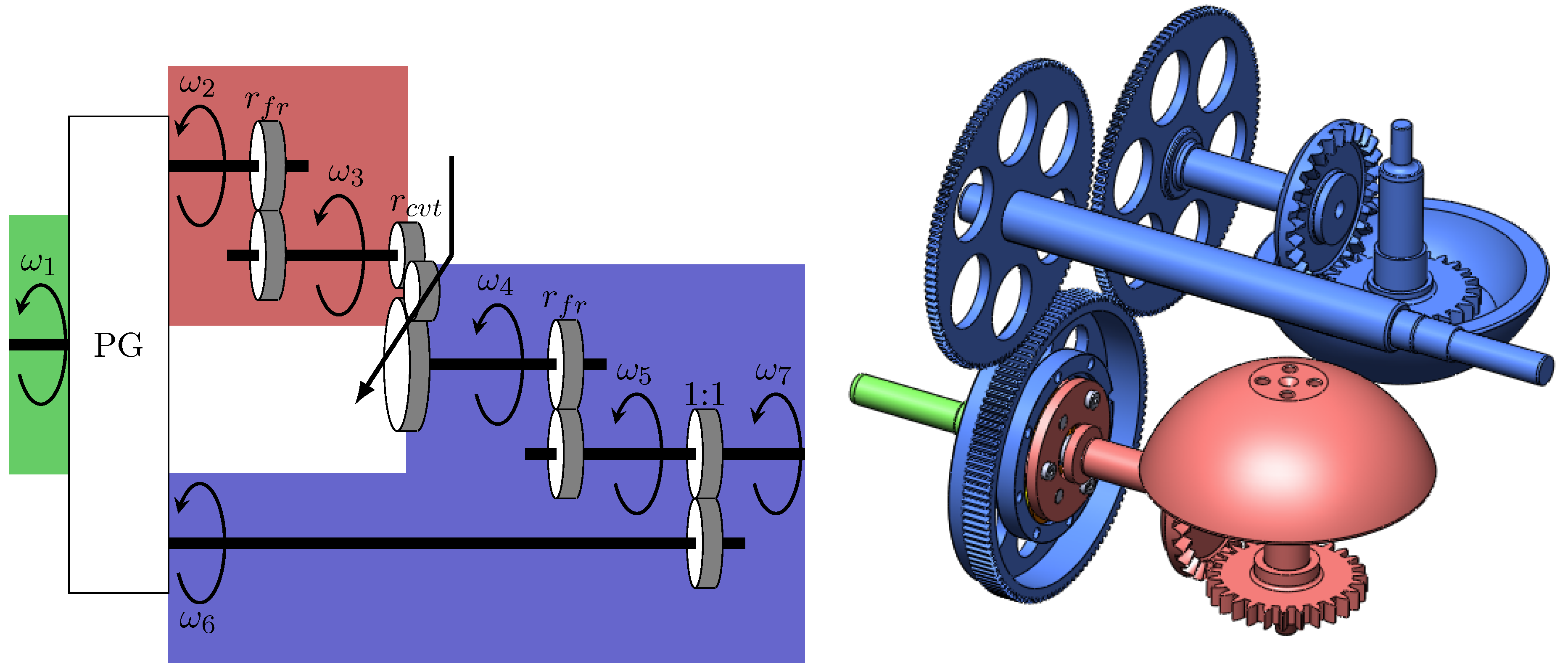
To enable the required bi-direction power flow and the corresponding transmission ratio range including positive and negative ratios, the power split principle is used as described in Section 2. Figure 3 shows a schematic drawing of the complete system and a preview of the mechanical realisation.
The transmission ratio of the power-split CVT (PS-CVT) is directly related to the transmission ratio of the CVT (), planetary gear (PG) and fixed ratio transmissions () as illustrated in Figure 3a. The transmission ratio of the CVT (), PS-CVT () and the remainder gears with constant ratio () are related to the angular velocity of each component ( to ) identified by the numbers 1 to 7 from Figure 3a.
Moreover, the kinematic relation between the rotation velocity of the sun gear (), carrier () and the annulus gear () of the planetary gear system is given by [10]:
with where is the radius of the annulus gear and the radius of the sun gear. In order to obtain the widest transmission ratio range including positive and negative ratios, the carrier is connected to component 6, the annulus to component 2 and, consequently, the sun to 1. This results into the kinematic relation for the planetary gear system according to
Finally, from Equations (2)–(4) and (6) and by considering , the transmission ratio of the PS-CVT is given by:
When typical planetary gear systems with are considered and a ratio of is selected, this equation reduces to
The resulting transmission ratios for typical values of are given in Figure 4.
Following from Figure 4, the transmission allows a bi-direction power flow and the corresponding required positive and negative transmission ratios for properly chosen values of and when the configuration angle is set over a range rad (property 1).
4. Dual-Hemi CVT Design Details
In order to experimentally validate the characteristics of the power split based dual hemispherical continuously variable transmission, a prototype has been built. To obtain a practical volume, the maximum allowable radius of the hemispherical friction wheels is set at 60 mm. The ratios for the planetary gear () and fixed ratio transmissions () are shown in Table 1. The resulting range of transmission ratios according to Equation (7) is given in Figure 5.
A schematic image of the PS-CVT is shown in Figure 6.
4.1. PS-CVT Torque Distribution
In order to determine the maximum allowable output torque of the PS-CVT, the internal torque distribution ( to ) must be considered. The ratio of torques belonging to the planetary gear system are directly related to its geometric relations and can be calculated as the dual of Equation (6) which results in Equations (9) and (10).
Furthermore, the ratio of torques for the CVT depend on the configured transmission ratio and can be calculated as the dual of Equation (3) which results in Equation (11).
The torque ratio of the remainder gear with constant transmission ratio can be calculated as the dual of Equation (4), which results in Equation (12).
By combining Equations (9)–(12), the internal torque distribution proportionally to the input torque () can be determined according to
As the resulting output torque is the resultant from the torque and , the output torque is given by:
For designing the DH-CVT, the transmitted torque through the CVT ( or ) is of main interest. According to Equation (14), the torque which passes through the CVT is directly related to and and the provided input torque .
4.2. Design of the Friction Wheels
To design the friction wheels, allowable ranges of transmission ratios and input torque that can be used without failure/slip of the CVT have to be determined. To do this, we assume that the output is fixed () such that the blue sphere cannot rotate. Then the force that the friction patch needs to hold, , is the force that is exerted on the blue sphere by the red sphere. This force is equal to the torque exerted on the red sphere, , divided by the effective radius of the red sphere, , and is equal to:
which results into
when combined with Equation (14).
The minimal preload in order to obtain the required friction contact is then given by
For practical reasons, hardened steel (100Cr6) is used as material. For a typical uncontaminated steel-on-steel contact, . Furthermore, the maximum allowable preload is bounded by the maximum allowable contact stress, in order to prevent failure in the contact region. The hertzian contact pressure between two spherical elements is given by [15]:
with
where represents the sphere radii of the two spheres and E and the E-modulus and the Poisson ratio of 100Cr6, respectively ( GPa, ). is the maximum allowable contact stress which we limited to 1.5 GPa.
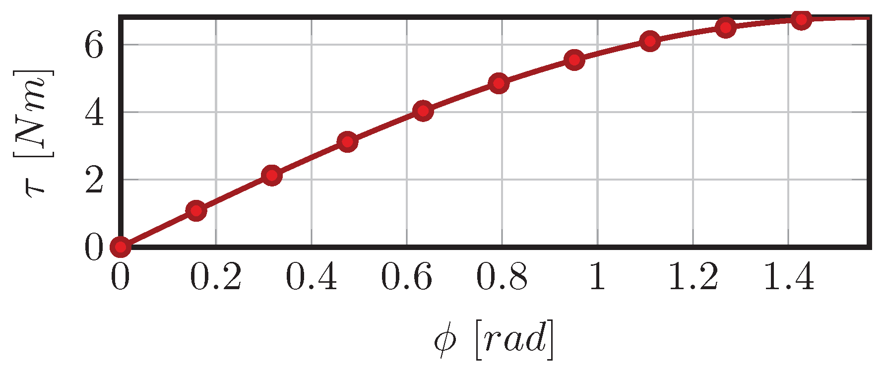
When combining Equations (21) and (22) and assuming , the maximum allowable input torque is directly related to configuration angle according to
Given and according to Table 1, the resulting maximum allowable input torque versus configuration angle is plotted in Figure 7.
As shown in Figure 7, slip is inevitable at a configuration of rad, as this would require an infinite preload or zero input torque. In order to prevent slip, the configuration angle should always remain sufficiently distant from rad.
Based on this figure, a minimum configuration angle of rad GAF: ik heb er +0.35 van gemaakt; er stond −0.35 is selected, resulting in an maximum allowable input torque of 2 Nm. In order to obtain a symmetric range of transmission ratios, a range of angles from rad to rad is selected.
5. Realisation
In this section, we discuss the realisation of the Dual-Hemi CVT in two steps. First, the drive train is discussed and, second, the reconfiguration mechanism.
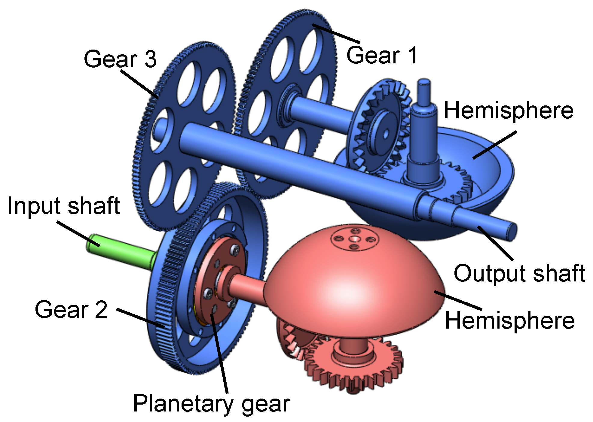
5.1. Drive Train
The drive-train of the Dual-Hemi CVT is shown in Figure 9.
At the heart of the mechanism, the two hemispheres can be found. The bearing system of the blue hemisphere is suspended and preloaded by disc-springs in order to obtain the required preloading force between both hemispheres. As this preload will induce small deformations of the hemispheres, small axial displacements will arise. Face-gears are used to ensure proper alignment of the gears connected to the hemispheres despite axial shift. These face-gears are connected to shafts that run exactly trough the center of the spheres. The shaft of the red hemisphere is connected to the ring gear of the planetary gear; the blue hemisphere’s shaft is connected to “gear 1”. The pitch diameter of “gear 1” is set equal to the diameter of the the hemispheres, as is the pitch diameter of “gear 2”, which is connected to the planet cage of the planetary gear. This ensures that “gear 1” can roll over “gear 2” when the blue hemisphere rolls over the red one to change the transmission ratio. The “output” shaft is connected to “gear 3”, which has the same diameter as “gear 2”. The “input” shaft is connected to the sun gear of the planetary gear.
5.2. Reconfiguration Mechanism
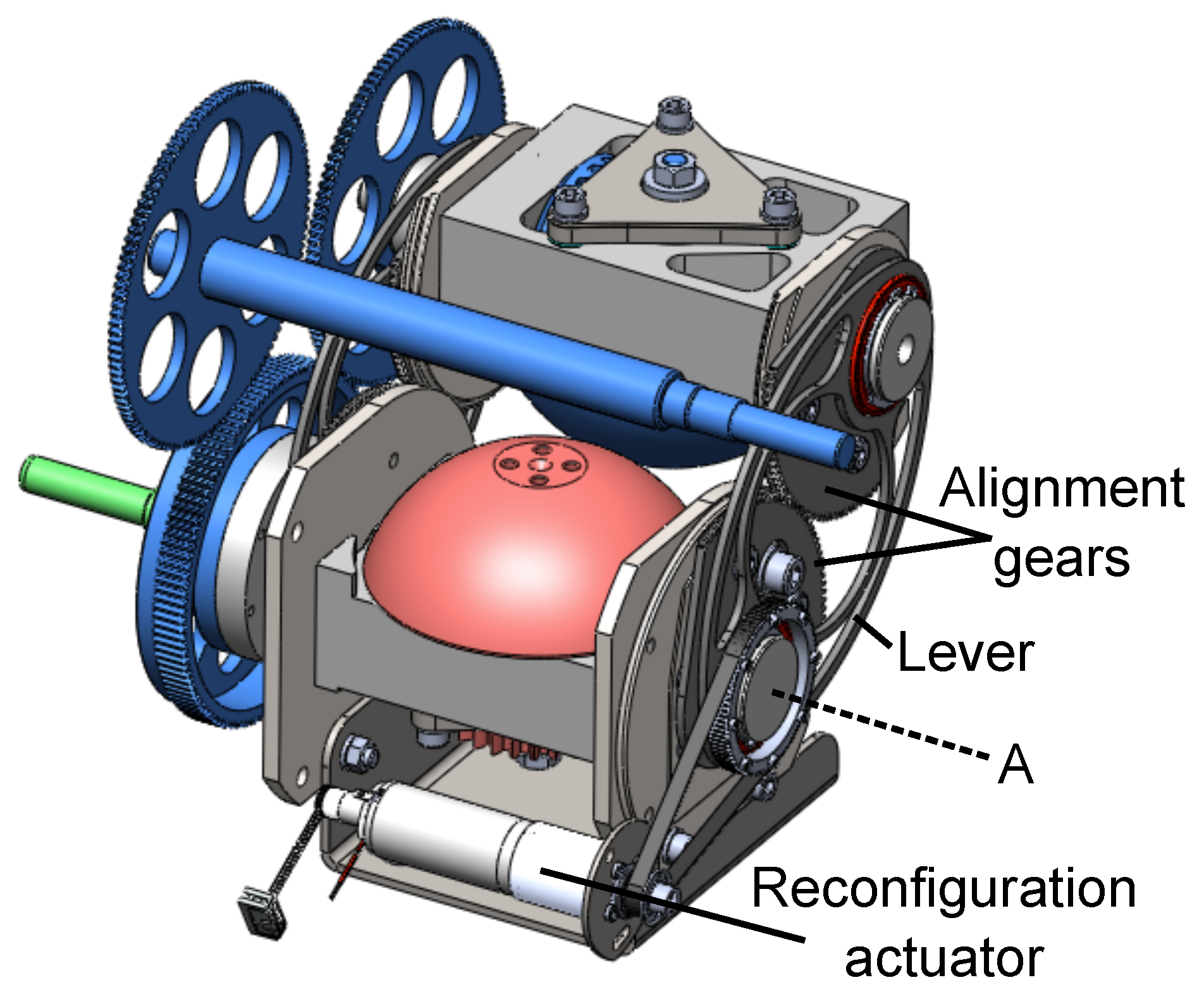
The reconfiguration mechanism is shown in Figure 10.
By using the “reconfiguration actuator”, the “lever” is rotated around point “A” with a timing belt. The “lever” has a length of twice the radius of the hemispheres. Referring to Figure 1a, it corresponds to the dash-dotted line between the centers of the red hemisphere and the blue sphere. The “alignment gears” have a pitch radius that is equal to the radius of the spheres and are an extra measure to make the blue hemisphere roll neatly over the red hemisphere when the “lever” is adjusted.
In order to reduce the required work for the reconfiguration mechanism, a spring-based gravity compensator (not shown in the figure) is added to compensate for the gravitational forces acting on the reconfiguration mechanism.
Figure 11 shows a picture of the setup.
6. Characterisation of the Setup
In this section, we discuss the characterisation of important parameters of the system. We start with the transmission system, based on a simplified lumped-parameter model of the systems, where each lumped parameter represents a quantity that will be characterised. Then we discuss the properties of the reconfiguration mechanism, based on which we can say something about the achievable bandwidth.
6.1. The Transmission System
Figure 12 shows a lumped IPM model of the transmission system.
In this model, the total inertia of the system is lumped in three elements: gm, gm, gm. The inertias are obtained from the CAD model of the CVT.
We are interested in the friction behaviour as seen at the output, therefore we carry all friction elements across the transmissions to lump them together at the output in an element . This process is discussed in detail next.
6.1.1. Friction
Based on observations, we assume a friction model that involves stiction and coulomb friction as shown in Figure 13, or:
As the friction is modelled as a lumped element at the output of the CVT, it is expected to be dependent on the transmission ratio, . Looking at Figure 3a while assuming stiction-coulomb friction at the points 1...7 and using Equations (13)–(18), a lumped friction element at the output would be of the following form:
where
and where is given by Equation (25).
We can also deduce:
such that:
With this, we can rewrite Equation (26) to:
which is of the form:
with different coefficients, a,b and c for:
Since and , only the bottom two of these are reached in practice. Therefore, we can expect different coefficients for:
In conclusion, we expect to find different parameters in the following four situations:
- and
- and
- and
- and
for both stiction and coulomb friction.
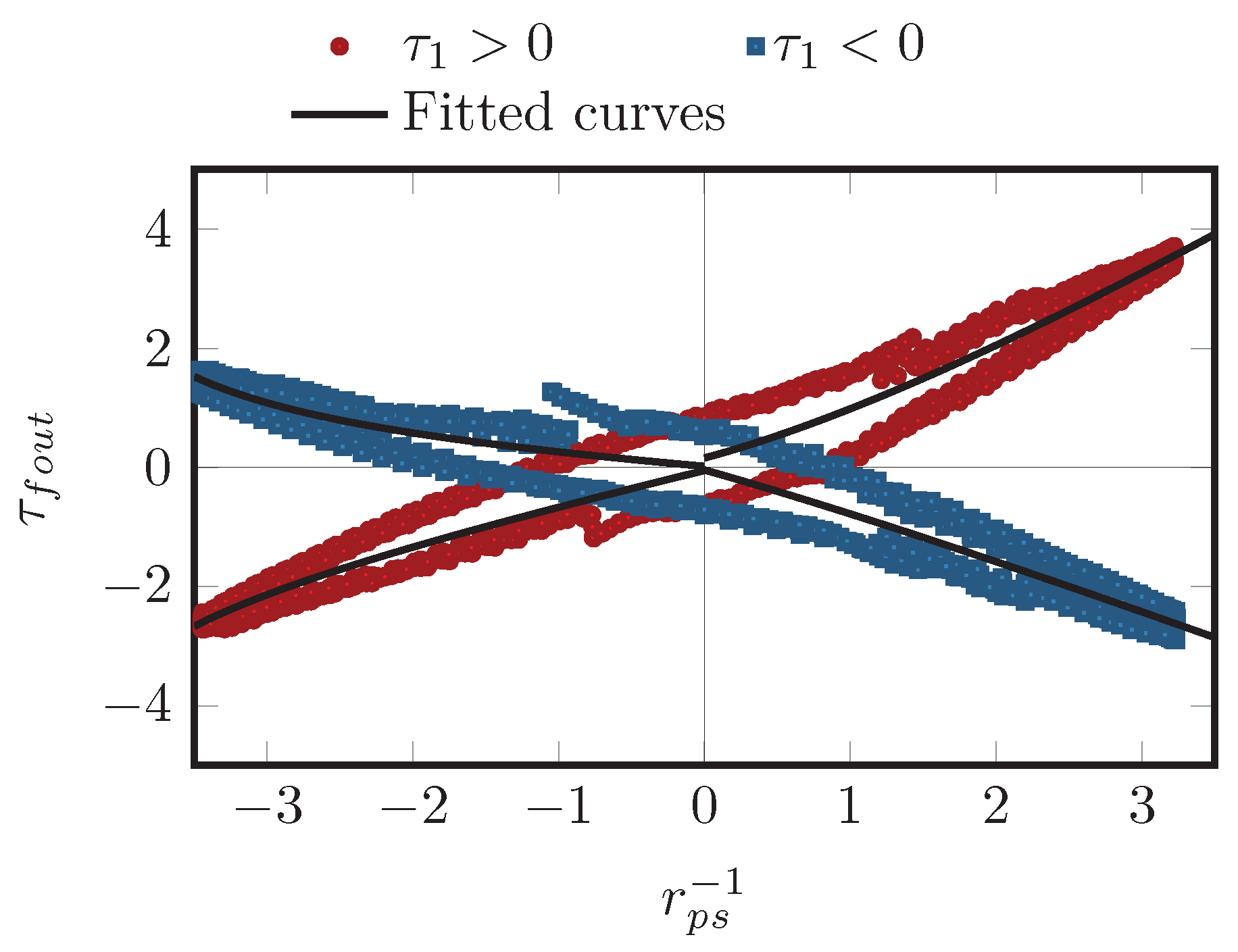
Parameter Identification: Stiction
To identify the parameters in the relation between stiction and the transmission ratio, we fixed the output of the PS-CVT with a torque sensor (). We applied a constant, known torque on the input () and varied the transmission ratio over the full range (). The torque that is measured at the output is equal to:
As , and are known, the friction torque can be calculated. Since , we measure stiction.
The result of this measurement is shown in Figure 14 together with the fitted curves. In this graph a positive corresponds to a positive output velocity.
The coefficients (a,b,c) of the fitted curves are given by:
In the measurements an hysteresis effect is present. The shape of the hysteresis varies with the rate at which the transmission ratio is changed. We have the following hypothesis on the cause of this effect: for different relative orientations of the spheres, a different pre-tension is exerted on the spheres, due to deformational effects. Related to this, the spheres have a different extent of deformation and the springs that provide the pre-tension have a different state. As the state of the springs change, the sphere has to move slightly. Special bearings have been applied to allow this, but they only work well with sufficient rotation. In the case of these experiments there is no rotation at all—since the goal is to measure stiction—making it difficult for the sphere to move. When changing the transmission ratio with a higher rate, the relative orientation also changes with a higher rate, such that the sphere has less time to move. This can cause a variation in pre-tension, which causes a variation in friction.
Unfortunately, we do not have the means to test this hypothesis.
Parameter Identification: Coulomb Friction
To identify the parameters in the relation between the coulomb friction and the transmission ratio, a servo motor was fixed to the output of the CVT and driven at a constant velocity (). A torque sensor was used to measure the torque that was applied to the system to maintain this velocity. This torque is equal to the friction torque plus torque required to speed up and slow down internal parts of the CVT. The contribution of the latter is insignificant (<0.00354 Nm) compared to the friction torque. The transmission ratio was varied over the full range (). Since , we measure coulomb friction.
The results are shown in Figure 15.
The coefficients (a,b,c) of the fitted curves are given by:
6.1.2. Efficiency
Based on the coulomb friction that was identified in the setup, we can say something about the efficiency. The maximum input torque, , is 2 Nm. The ideal, lossless, output torque, , is given by:
The actual output torque, , is equal to:
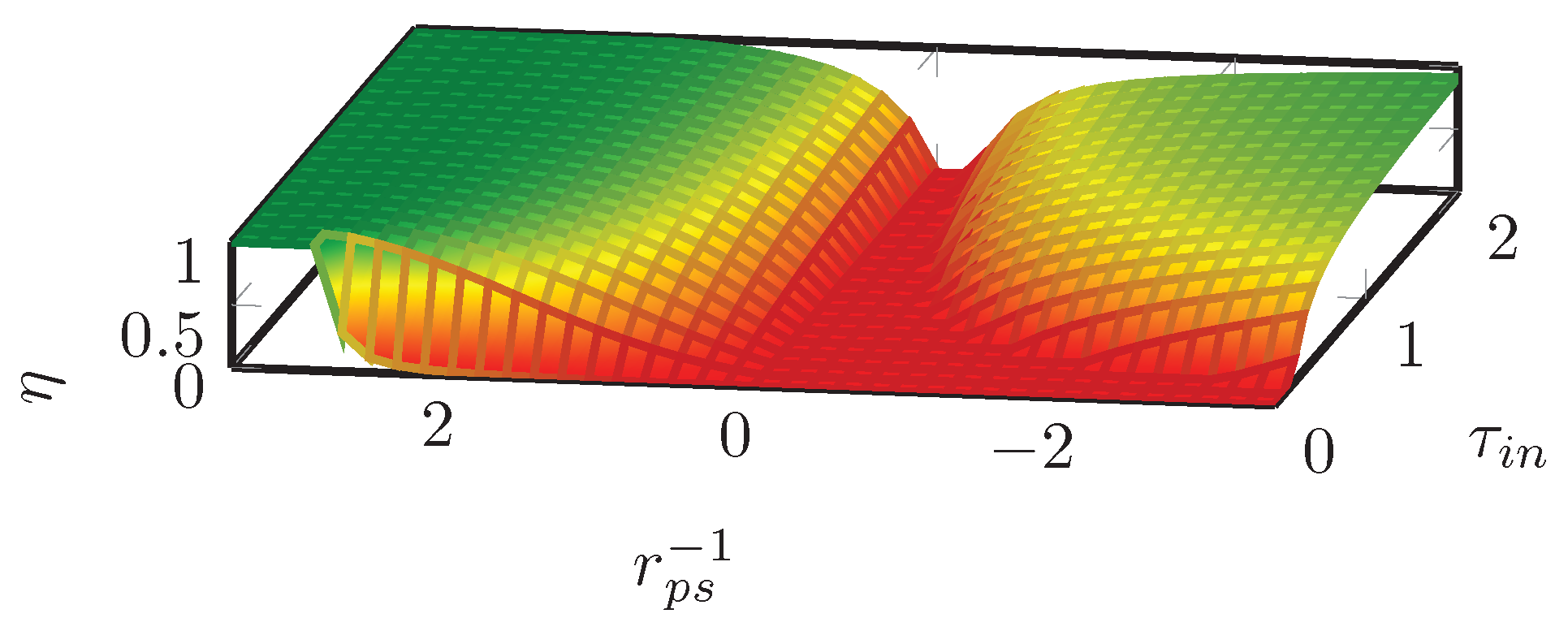
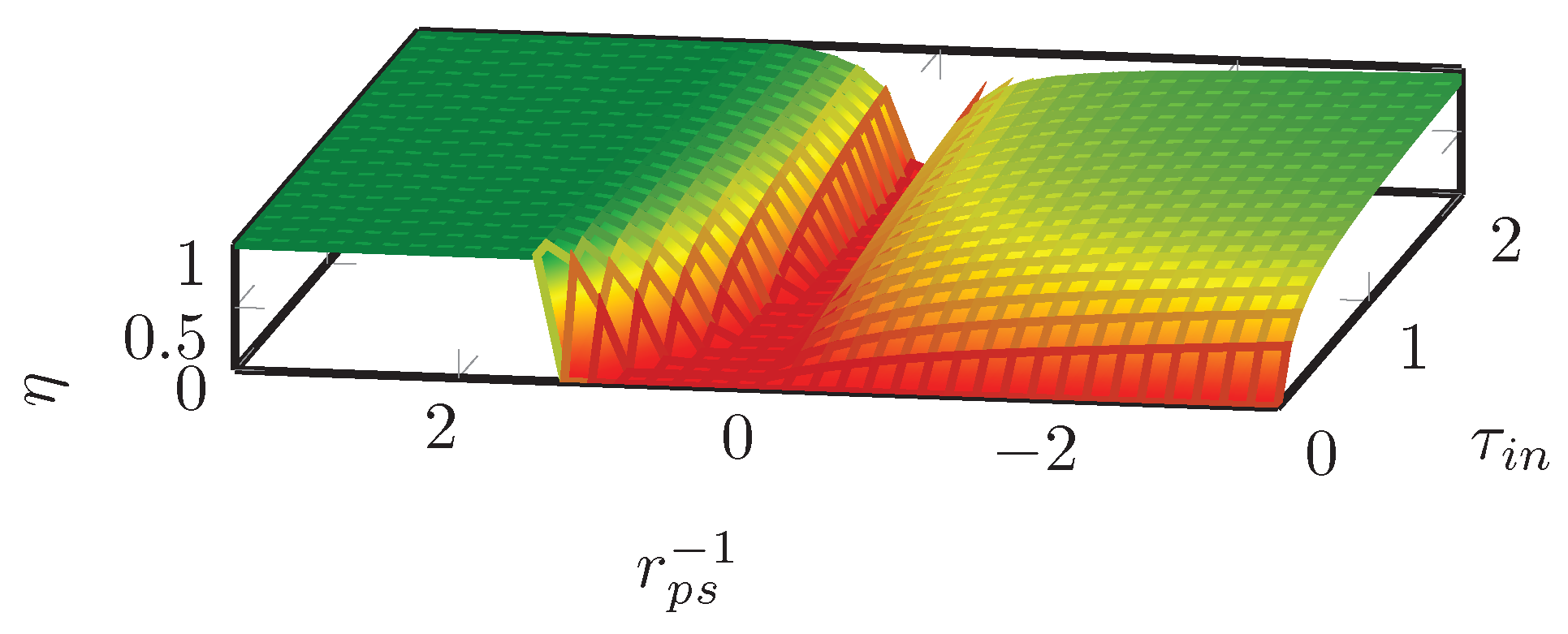
When delivering energy (), the efficiency, , is given by:
When recovering energy (), the efficiency, , is given by:
6.2. Reconfiguration Mechanism
Figure 18 shows a lumped model of the reconfiguration mechanism.
The transmission ratio was determined experimentally by rotating the output shaft with a constant velocity and measuring the velocity at the input () and output (), while changing the transmission ratio over the full range. Figure 19 shows the experimentally determined transmission ratio with the theoretical relation. The difference is small.
6.2.1. Bandwidth
The total inertia of the reconfiguration system as seen from the input is equal to kgm. On this inertia, three torques act: a torque exerted by the gravity-compensating spring , a torque exerted by gravity and a torque exerted by the reconfiguration actuator . The total torque that is applied to the inertia, is equal to:
The torque that is contributed by gravity, , is equal to:
where ms is the gravitational acceleration constant, kg the mass of the system, m the length of the arm and the angle to of the mechanism as shown in Figure 18.
The torque that is contributed by the gravity compensating spring, , equal to:
is the length of the spring, the orientation of the spring, N the minimum force that is required to elongate the spring, m the rest length of the spring, Nm the stiffness of the spring and m, m the location of the point P relative to the hinge point as shown in Figure 18.
Assuming no friction losses, the reconfiguration actuator can deliver up to Nm.
Figure 20 shows the maximum torque that can be applied to accelerate the inertia of the reconfiguration mechanism for all .
This shows that at any angle , we can at least apply Nm to accelerate the reconfiguration mechanism.
The general concept of bandwidth cannot be applied but we take a pragmatic approach to get a viable estimate.
Suppose is a sinusoid:
then the acceleration is also a sinusoid:
with amplitude .
Our maximum torque of Nm results in a maximum acceleration of:
So
We know that A lies within the range of the mechanism, . Assuming we don’t restrict the range, we obtain:
which gives an estimate for the “bandwidth” of the system.
7. Discussion and Exploration
In this section, we discuss two parameters that can be changed in the design of the DH-CVT to achieve different results: the maximum allowable output torque and the ratio of the fixed ratio transmissions. In addition we discuss how different ratio ranges can be achieved.
7.1. Scaling of the System with Output Torque
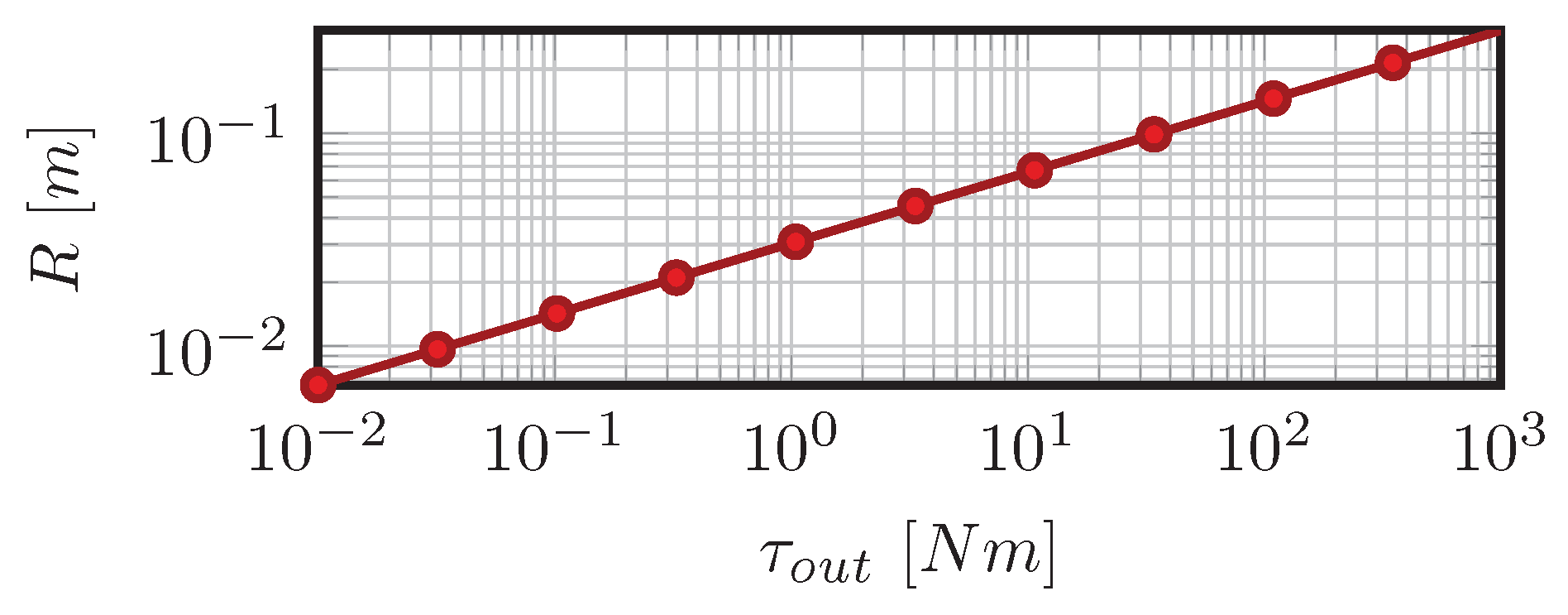
For the discussed realisation of the DH-CVT, dimensions of the friction spheres are chosen at 60 mm radius for practical reasons. However, the spheres could be scaled in order to achieve a different maximum allowable output torque. By combining Equations (18) and (24), a relation can be obtained between the minimum required sphere radius and the maximum allowable output torque. Since the sphere radius (R) scales to the third power with the maximum input and output torque, an increase of a factor ten of the sphere radius results in an increase of a factor thousand of the output torque (Figure 21). In perspective, upscaling the considered system to increase output torque can be achieved rather easily for high-torque applications. However, downscaling the system to reduce dimensions would dramatically reduce the maximum output torque, making the considered variable transmission impractical for small robotic systems.
7.2. High Torque vs. High Velocity Power Transmission in the Spheres
The maximum output torque, , of the Dual-Hemi CVT is limited by the maximum allowable throughput torque at the friction spheres, , and the kinematic relations of the system, Equations (13)–(17) as explained in Section 4.2. By increasing the fixed ratio transmissions (), the throughput torque of the spheres can be reduced (Equation (14)). When reducing the throughput torque of the spheres, the required preload on and the radius of the spheres can be reduced (Equation (21)).
Reducing the radius of the spheres reduces their inertia and enables reducing the size and weight of both the reconfiguration mechanism—yielding a higher bandwidth (Section 6.2.1)—and the complete system. On the other hand, the effect of the inertia on the system scales quadratically with .
Reducing the preload reduces the load on the bearings and thus frictional forces at the bearings. In addition to this, the increased rotational velocity may further reduce the losses in the bearings [16]. On the other hand, the impact of the frictional forces on the system scales quadratically with .
Summing up, increasing the ratio of the fixed-ratio transmission is expected to reduce the size of the system and have a favourable effect on the bandwidth of the reconfiguration mechanism. Wether or not it has a favourable effect on the total inertia and friction of the system requires closer examination.
7.3. Obtaining a Different Ratio Range
For the design discussed in this work, a ratio range of was chosen. Equation (7) shows how the ratio is related to the angle of the spheres, the fixed ratio transmission and the ratio between the radius of the annulus and sun gears of the planetary gear. By selecting different values for these parameters, different ratio ranges can be achieved.
8. Conclusions
In this work, the Dual-Hemi CVT is presented. It is a novel CVT, designed to have properties that we believe are required to apply continuously variable transmissions to their full potential in robotics. We discussed the most important design details and a characterization of the system. We show that the system has all the aforementioned required properties.
The ratio range includes positive, negative and an infinite ratio, the system is fully back-drivable under all conditions and the reconfiguration action is completely decoupled from the transmission action.
In Section 6.1.2 we showed that the efficiency is between and for a large part of the operation range of the CVT. The efficiency quickly drops to zero when the inverse transmission ratio, , or the input torque approaches zero. The significance of the work required for reconfiguration is application-dependent and will be studied in future work.
When looking at the friction properties of the system in Section 6.1.1, we see that stiction is significantly higher than coulomb friction. In combination with the relatively low bandwidth discussed in Section 6.2.1, this may cause problems in terms of controlling the output torque.
In the discussion in Section 7, we have shown that this specific design of the CVT will have significantly more beneficial properties when scaling up, while it will have significantly less beneficial properties when scaling down.
Using a different (higher) ratio for the fixed transmissions is expected to reduce the size of the system and the inertia of the reconfiguration mechanism, resulting in an increased bandwidth. It may or may not have a nett favourable effect on the friction and inertia of the system.
Acknowledgments
This work was financed by the Dutch Technology Foundation STW under grant 10550.
Author Contributions
Douwe Dresscher performed the experiments, interpreted data, wrote the manuscript and acted as corresponding author. Mark Naves significantly contributed to the design of the Dual-Hemi CVT and contributed to writing the manuscript. Theo J. A. de Vries supervised development of work, helped in data interpretation and manuscript evaluation. Martijn Buijze supervised the development of the Dual-Hemi CVT. Stefano Stramigioli helped to evaluate and edit the manuscript.
Conflicts of Interest
The authors declare no conflict of interest. The founding sponsors had no role in the design of the study; in the collection, analyses, or interpretation of data; in the writing of the manuscript, and in the decision to publish the results.
References
- Beachley, N.; Frank, A. Continuously Variable Transmissions: Theory and Practice; No. UCRL-15037; Lawrence Livermore Lab., California University: Livermore, CA, USA, 1979. [Google Scholar]
- Ansink, J. Design and Analysis of an Infinitely Variable Transmission for Energy Efficienct Actuation; Technical Report; University of Twetne: Enschede, The Netherlands, 2008. [Google Scholar]
- Lahr, D. Development of a Novel Cam-Based Infinitely Variable Transmission; Technical Report; Virginia Polytechnic Institute and State University: Blacksburg, VA, USA, 2009. [Google Scholar]
- Groothuis, S.; Rusticelli, G.; Zucchelli, A.; Stramigioli, S.; Carloni, R. The vsaUT-II: A novel rotational variable stiffness actuator. In Proceedings of the 2012 IEEE International Conference on Robotics and Automation, St Paul, MN, USA, 14–18 May 2012; pp. 3355–3360. [Google Scholar]
- Jafari, A.; Tsagarakis, N.G.; Vanderborght, B.; Caldwell, D.G. A novel actuator with adjustable stiffness (AwAS). In Proceedings of the 2010 IEEE/RSJ International Conference on Intelligent Robots and Systems, Taipei, Taiwan, 18–22 October 2010; pp. 4201–4206. [Google Scholar]
- Jafari, A.; Tsagarakis, N.G.; Caldwell, D.G. AwAS-II: A New Actuator with Adjustable Stiffness based on the Novel Principle of Adaptable Pivot Point and Variable Lever Ratio. In Proceedings of the IEEE International Conference on Robotics and Automation, Shanghai, China, 9–13 May 2011; pp. 4638–4643. [Google Scholar]
- Kim, B.S.; Song, J.B. Hybrid Dual Actuator Unit : A Design of a Variable Stiffness Actuator based on an Adjustable Moment Arm Mechanism. In Proceedings of the IEEE International Conference on Robotics and Automation, Anchorage, AK, USA, 3–7 May 2010; pp. 1655–1660. [Google Scholar]
- Peshkin, M.; Colgate, J.; Wannasuphoprasit, W.; Moore, C.; Gillespie, R.; Akella, P. Cobot architecture. IEEE Trans. Robot. Autom. 2001, 17, 377–390. [Google Scholar] [CrossRef]
- Everarts, C.; Dehez, B.; Ronsse, R. Novel infinitely Variable Transmission allowing efficient transmission ratio variations at rest. In Proceedings of the 2015 IEEE/RSJ International Conference on Intelligent Robots and Systems (IROS), Hamburg, Germany, 28 September–2 October 2015; pp. 5844–5849. [Google Scholar]
- Bottiglione, F.; Mantriota, G. Reversibility of Power-Split Transmissions. J. Mech. Des. 2011, 133, 084503. [Google Scholar] [CrossRef]
- Dresscher, D.; de Vries, T.J.; Stramigioli, S. Motor-gearbox selection for energy efficiency. In Proceedings of the 2016 IEEE International Conference on Advanced Intelligent Mechatronics (AIM), Banff, AB, Canada, 12–15 July 2016; pp. 669–675. [Google Scholar]
- Stramigioli, S.; van Oort, G.; Dertien, E. A concept for a new Energy Efficient Actuator. In Proceedings of the 2008 IEEE/ASME International Conference on Advanced Intelligent Mechatronics, Xi’an, China, 2–5 July 2008; pp. 671–675. [Google Scholar]
- Everarts, C.; Dehez, B.; Ronsse, R. Variable Stiffness Actuator applied to an active ankle prosthesis: Principle, energy-efficiency, and control. In Proceedings of the 2012 IEEE/RSJ International Conference on Intelligent Robots and Systems (IROS), Vilamoura-Algarve, Portugal, 7–12 October 2012; pp. 323–328. [Google Scholar]
- Dresscher, D.; de Vries, T.J.; Stramigioli, S. Inertia-Driven Controlled Passive Actuation. Proceedings of ASME 2015 Dynamic Systems and Control Conference, Columbus, OH, USA, 28–30 October 2015; p. V003T45A002. [Google Scholar]
- Hertz, H. Ueber die Berührung fester elastischer Körper. J. Reine Angew. Math. 1882, 92, 156–171. (In German) [Google Scholar]
- Blake, P.W.R. Lubrication of Rolling Bearings. Tribol. Int. 1976, 9, 53. [Google Scholar] [CrossRef]
Figure 1.
A conceptual drawing of the Dual-Hemi CVT. To change the transmission ratio, the blue hemisphere rolls over the red one around the x-axis of the frame in the point of contact (black dot in the figure). (a) An overview drawing of the conceptual mechanism. (b) A zoom on the contact point, with the addition of frame . (The initial idea of the Dual-Hemi CVT is by Peter Rutgers, DEMCON, Enschede, The Netherlands.)

Figure 2.
The complete transmission ratio range of the DH-CVT.
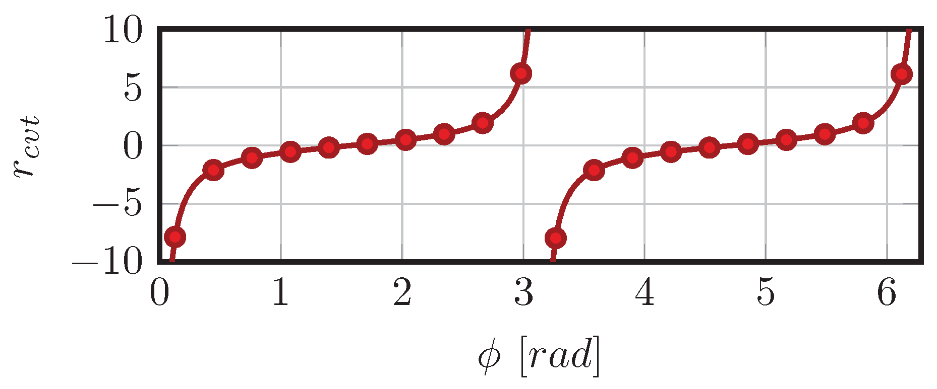
Figure 3.
Schematic overview of a PS-CVT and a preview of the mechanical realisation (will be discussed in depth in Section 5). The colour coding illustrates the relation between parts in the schematic figure the drawing of the mechanical system. The parts connected to the ring gear of the planetary gear are blue, the parts connected to the cage of the planets of the planetary gear are coloured red and the parts connected to the sun gear of the planetary gear are coloured green. (a) Schematic overview of a PS-CVT. (b) Drawing of the mechanical system.

Figure 4.
Transmission ratio of PS-CVT for typical values of .
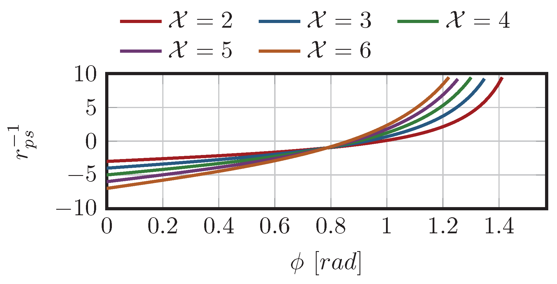
Figure 5.
Transmission ratio of PS-CVT and DH-CVT.
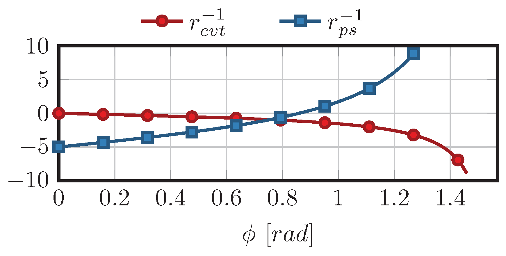
Figure 6.
A conceptual drawing of the Dual-Hemi CVT (left) in combination with a planetary gear (right). The fixed ratio transmissions are not shown.
Figure 6.
A conceptual drawing of the Dual-Hemi CVT (left) in combination with a planetary gear (right). The fixed ratio transmissions are not shown.

Figure 7.
Maximum allowable input torque .

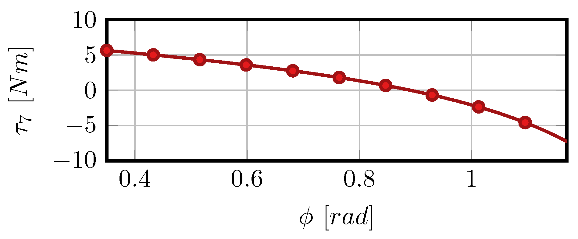
Figure 8.
Output torque over the selected configuration range.

Figure 9.
An image showing the drive train of the dual-hemi CVT. The use of colours is consistent with Figure 6: the parts connected to the ring gear of the planetary gear are blue, the parts connected to the cage of the planets of the planetary gear are coloured red and the parts connected to the sun gear of the planetary gear are coloured green.

Figure 10.
An image showing the drive train and reconfiguration mechanism of the dual-hemi CVT.

Figure 11.
A photo of the Dual-Hemi CVT. Photo by Wanda Tuerlinckx.
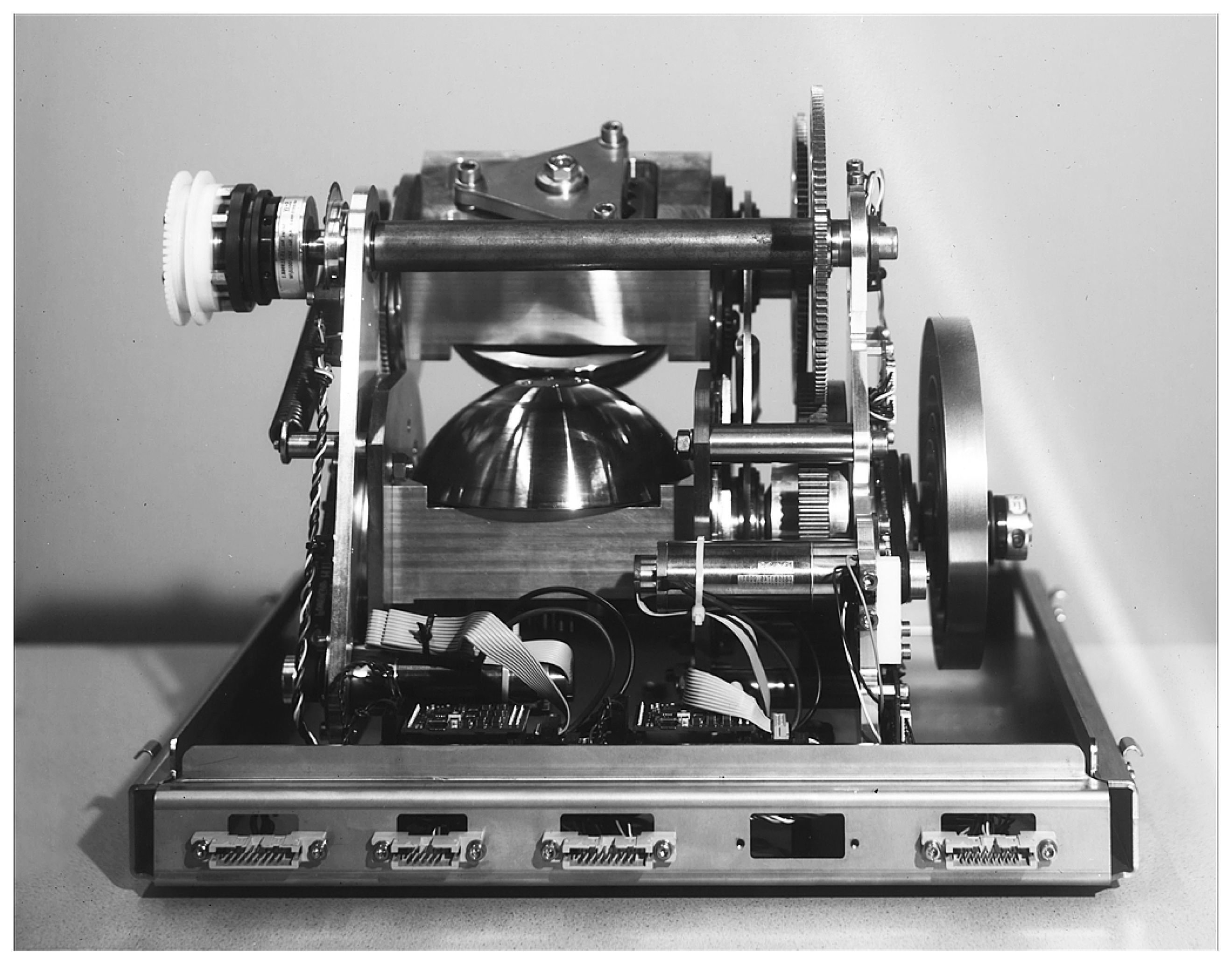
Figure 12.
Simplified IPM of the transmission system.
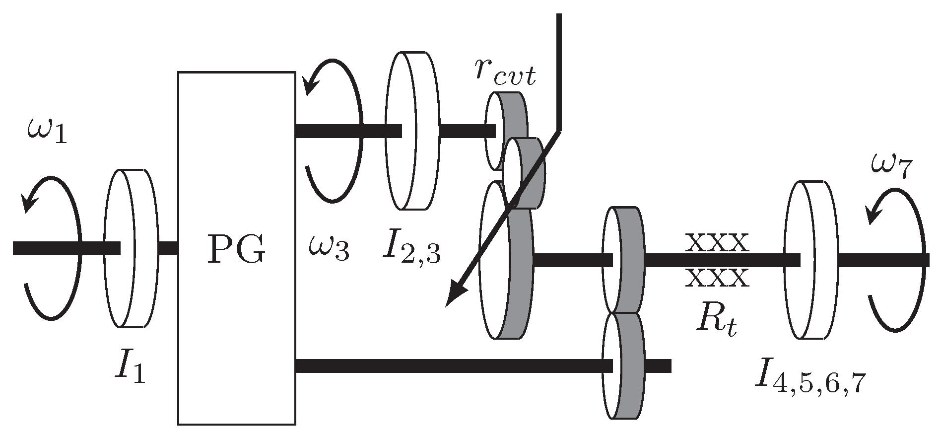
Figure 13.
Friction model.
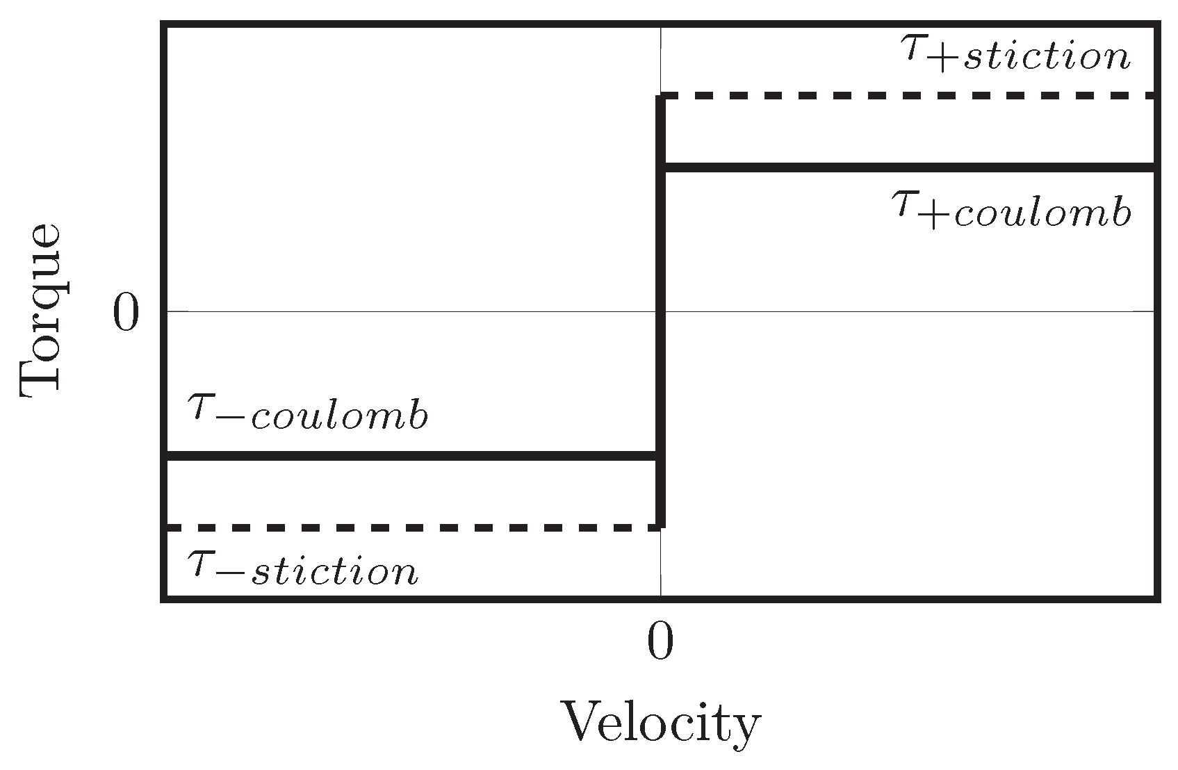
Figure 14.
Stiction, measurements and fitted curves.

Figure 15.
Coulomb friction, measurements and fitted curves.

Figure 16.
Efficiency for negative output velocities.

Figure 17.
Efficiency for positive output velocities.

Figure 18.
Schematic illustration of the reconfiguration mechanism.
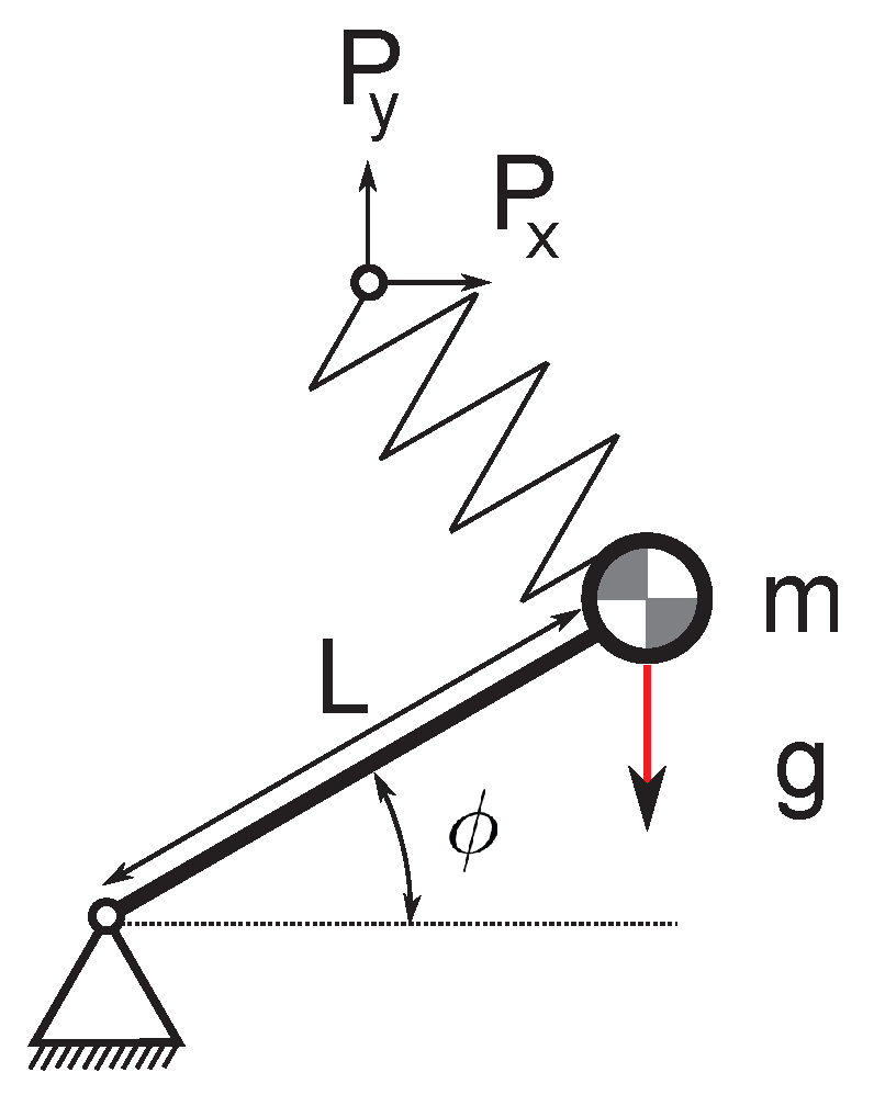
Figure 19.
Inverse transmission ratio of the PS-CVT.
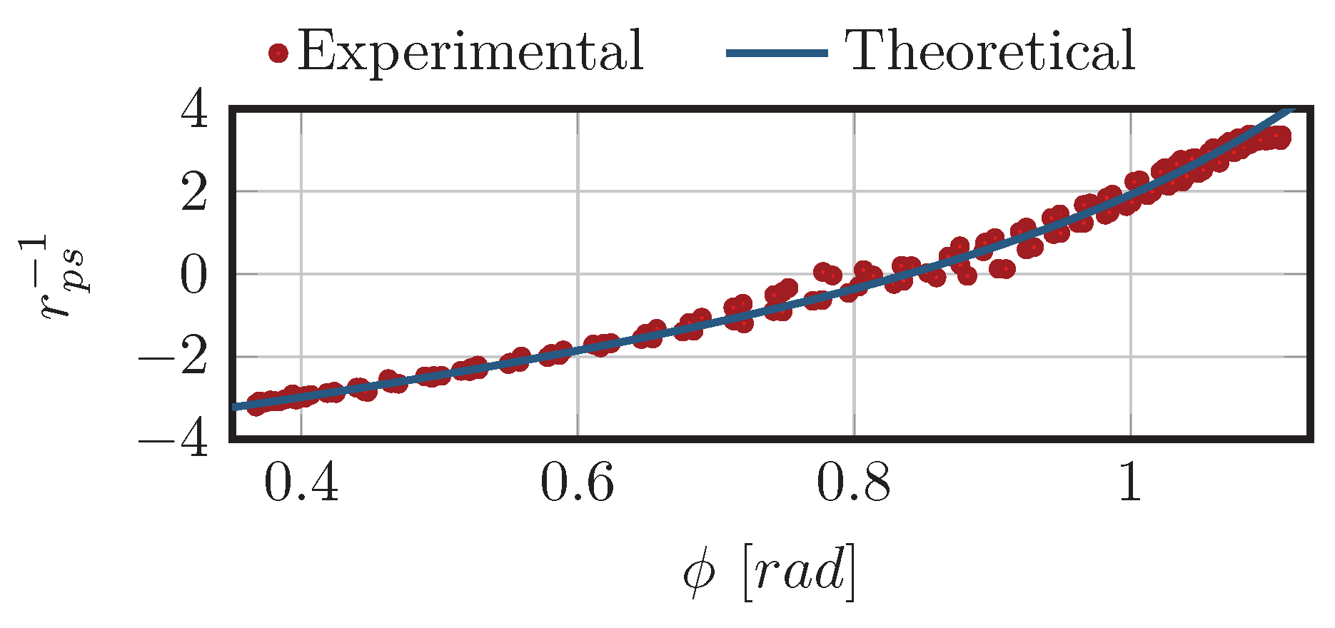
Figure 20.
Max magnitude of the torque that can be applied to the reconfiguration mechanism.
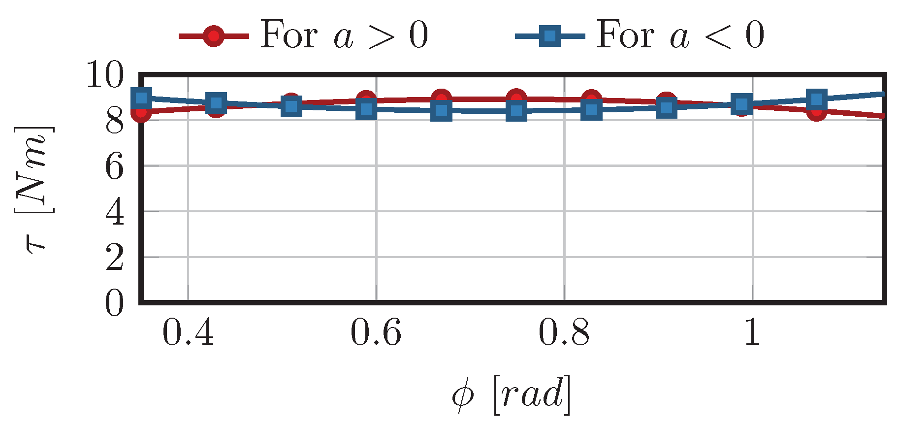
Figure 21.
Scaling of the friction wheel radius with output torque.


Table 1.
Planetary gear and fixed ratio transmission ratios.
| Parameter | Value |
|---|---|
| 4 | |
| −26/27 |
© 2017 by the authors. Licensee MDPI, Basel, Switzerland. This article is an open access article distributed under the terms and conditions of the Creative Commons Attribution (CC BY) license (http://creativecommons.org/licenses/by/4.0/).
Share and Cite
MDPI and ACS Style
Dresscher, D.; Naves, M.; De Vries, T.J.A.; Buijze, M.; Stramigioli, S. Power Split Based Dual Hemispherical Continuously Variable Transmission. Actuators 2017, 6, 15. https://doi.org/10.3390/act6020015
AMA Style
Dresscher D, Naves M, De Vries TJA, Buijze M, Stramigioli S. Power Split Based Dual Hemispherical Continuously Variable Transmission. Actuators. 2017; 6(2):15. https://doi.org/10.3390/act6020015
Chicago/Turabian StyleDresscher, Douwe, Mark Naves, Theo J. A. De Vries, Martijn Buijze, and Stefano Stramigioli. 2017. "Power Split Based Dual Hemispherical Continuously Variable Transmission" Actuators 6, no. 2: 15. https://doi.org/10.3390/act6020015
Note that from the first issue of 2016, this journal uses article numbers instead of page numbers. See further details here.