Optimization Design of Electromagnetic Actuator Applied as Fast Tool Servo

1
School of Mechanical Engineering, Tianjin University of Technology and Education, Tianjin 300222, China
2
Tianjin Key Laboratory of High Speed Cutting & Precision Machining, Tianjin University of Technology and Education, Tianjin 300222, China
3
Tianjin Institute of Metrological Supervision and Testing, Tianjin 300192, China
*
Author to whom correspondence should be addressed.
Actuators 2017, 6(3), 25; https://doi.org/10.3390/act6030025
Submission received: 21 June 2017
/
Revised: 6 August 2017
/
Accepted: 8 August 2017
/
Published: 18 August 2017
Abstract
:Fast tool servos (FTS) for single point diamond turning are widely employed for machine optical free-form surfaces. A FTS with a large stroke and a high bandwidth can increase the efficiency of a machine and complexity of a work-piece. In this paper, a FTS driven by a Maxwell electromagnetic actuator is developed to obtain a relatively large stroke and high bandwidth. In this study, a multi-objective optimization model is proposed based on the whole system by considering electromagnetic driving principles, kinematic model, and mechanical model. The proposed optimization model can be applied to solve the parameters of electromagnetic actuators with diverse application requirements. A sequential quadratic programming (SQP) algorithm is implemented to solve the problem. The optimization results are verified through both finite element analysis and experiments. The optimized FTS can produce 49.55 μm of full stroke with a frequency response of 3.2 kHz.
1. Introduction
Optical free-form surfaces are increasingly used in various areas, such as the aerospace, energy, and life science. The single-point diamond turning method based on the fast tool servo (FTS) system is widely adopted due to the advantages of high accuracy and superior process efficiency [1]. A wide variety of FTSs exist which employ different types of actuators [2]. These FTSs provide different strokes and bandwidths. The stroke of a FTS determines the non-rotationally symmetric component of a desired surface, while the bandwidth determines the productivity, surface complexity, and even the materials that can be processed by the machine [3]. A FTS with a larger stroke (several millimeters) and a higher bandwidth (several thousands of hertz) is necessary to process more complex surfaces of higher amplitude with machines. However, in reality, a large stroke and high bandwidth cannot be implemented at the same time. Therefore, different types of FTSs with different strokes and bandwidths were designed.
FTSs driven by piezoelectric actuators (PZT-FTS) [4,5], FTSs driven by Lorentz forces in the voice-coil motor (VCM-FTS) [6,7] and FTSs driven by Maxwell electromagnetic actuators (MEA-FTS) [8,9] have been widely studied by researchers. Based on different driving methods, different types of flexure-based mechanisms—such as flexure hinges, leaf springs, and levers—were applied to realize FTSs with specific strokes and bandwidths. Many researchers investigated optimization methods to solve the parameters of the flexures in their specialized FTSs [10,11,12,13,14].
Zhu et al. developed a two-dimensional FTS, which can obtain better profile accuracy and surface quality due to its novel adaptive tool servo (ATS) diamond turning method [10]. Yang et al. employed a commercialized PZT actuator to create their FTS [11]. A flexure optimization was performed based on the finite analysis model of commercial software ANSYS in their design. The optimized FTS was able to produce a stroke of 24.6 μm at a first resonant frequency of 2192 Hz. Zhu et al. fulfilled their requirements for a FTS by optimizing the parameters of a flexure hinge with the multi-objective method based on the differential evolution algorithm [12]. Their FTS produced a stroke of 10.25 μm with a first resonant frequency of 2000 Hz. Zhuang et al. proposed a multi-objective topology optimization method for the design of a compliant mechanism, with the proposed design showing better performance by increasing the effective stroke of FTS in addition to improving the stiffness in the vertical (main cutting force) and horizontal (feed force) directions [13]. Rakuff et al. used finite element analysis to optimize the parameters of their specially designed leaf flexure before adjusting the damping ratio of the FTS system with special experiments [14]. Their FTS completed ultra-precision machining successfully due to its characteristics of a 2 mm stroke and a bandwidth of 140 Hz. Most researchers focused on optimizing the design of flexures rather than the whole FTS system. However, a typical FTS system consists of both flexures and the actuator producing a driving force as well as the transmission unit. The ultimate performance of FTS depends on the whole system. Hence, both the optimization results and the ultimate performance of the optimized FTS are affected.
A survey of the literature shows that the optimizations of FTS structure were focused on flexures, despite flexures being only one part of the FTS system. The actuator, the tool holder, and other parts have not been considered for optimization in these studies, meaning that previous optimization was not based on the whole system. Thus it can be suggested that FTS has not been fully optimized and its best performance has not been reached.
Compared to PZT-FTS with the limitation of small stroke and VCM-FTS with the limitation of low bandwidth, the MEA-FTS can implement FTS at a larger stroke compared to PZT-FTS (at the same bandwidth) and a higher bandwidth compared to VCM-FTS (at the same stroke) [15,16]. According to a series of surveys, a fast tool servo driven by the electromagnetic actuator has the ability to obtain a relatively larger stroke and higher bandwidth compared to PZT-FTS and VCM-FTS. Figure 1 shows the characteristics of a series of FTSs. It shows the advantages of MEA-FTS. Similar conclusions have also been reported by Lu and Xie [15,16]. In this paper, MEA-FTS is studied and a multi-objective optimization model is built based on the driving model of electromagnetic actuator, mechanical structure, and kinematic model. The optimal parameters of the electromagnetic model and mechanical structure are solved. A generalized optimization model of MEA-FTS is proposed and the optimization model can be applied to many types of FTS at a variety of strokes and frequencies.
2. Materials and Methods
2.1. Construction of MEA-FTS Model
2.1.1. Electromagnetic Driving Model
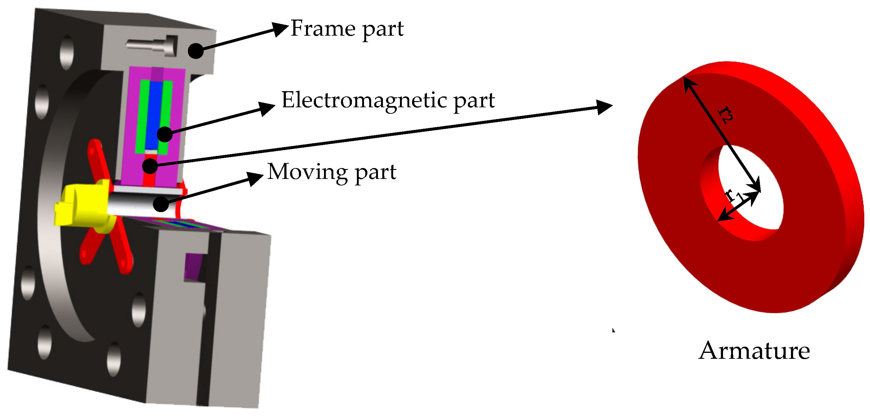
A 3D-model of MEA-FTS is shown in Figure 2. MEA-FTS consists of three parts: the frame, electromagnetic part, and moving part. The electromagnetic part produces the actuating force on the armature, while the moving part transforms the actuating force into specific movements.
The magnetic part consists of yokes, coil windings, a permanent magnet, armature, and air gaps between the yokes and armature. The magnetic part is a rotationally symmetrical 2D-model, which is shown in Figure 3. This magnetic part is used to analyze the electromagnetic principles. The permanent magnet produces a magnetic flux, which is shown in Figure 3 as the biasing flux. The exciting flux, shown in Figure 3, is produced by currents in the coil windings. MEA-FTS is driven by the Maxwell electromagnetic force, which involves the electromagnetic tension in air gaps [13]. The magnetic field in both air gaps consists of a flux density (BB) excited by the permanent magnet and a flux density (BE) excited by the currents in coil windings. Assuming that the flux density in yokes is not saturated, we define the Maxwell electromagnetic force acting on the left side of armature as Fl; the Maxwell electromagnetic force acting on the right side of armature as Fr; the flux density in the left air gap as Bl; and the flux density in the right air gap as Br. The magnetic fields in both air gaps are consistent with the superposition theorem. Therefore, we can conclude the following: Br = BBr + BE and Bl = BBl − BE. We define BBr as the flux density excited by the permanent magnet in the right air gap and BBl as the flux density excited by the permanent magnet in the left air gap. When the displacement of the armature is z, the actuating Maxwell force can be calculated according to the equation [17]
where z0 is the air gap when the armature is in the middle of the model; z is the displacement of the armature (unit: m); BB is the magnetic flux density generated by the permanent magnet (unit: T); S is the yoke pole face area at each working gap (unit: m2); μ0 is the permeability of air (μ0 = 4π × 10−7 N/A2); N is the number of turns in the coils; and I is the exciting current (unit: A).
The formula of the maximum driving force should be derived to estimate the stroke of MEA-FTS. According to Equation (1), the maximum driving force can be derived through Equation (2)
The actuating force reaches its maximum when the flux density in the yoke becomes saturated (B = Bsat, where Bsat is the saturated flux density) with maximum displacement of the armature (z = z0, where BBr = BBl). We define the outer radius of the armature as r2 and the inner radius of armature as r1. Therefore, the yoke pole face area at each working gap is S = π(r22 – r12). The maximum actuating force can be derived as Equation (3)
According to Equation (3), the maximum driving force is proportional to the squared value of Bsat squared. Thus, the Kool Mμ is chosen according to the magnetic material of the yokes and armature. The saturation flux density of Kool Mμ is 1.4 T, while the relative permeability is 125.
2.1.2. Mechanic Model
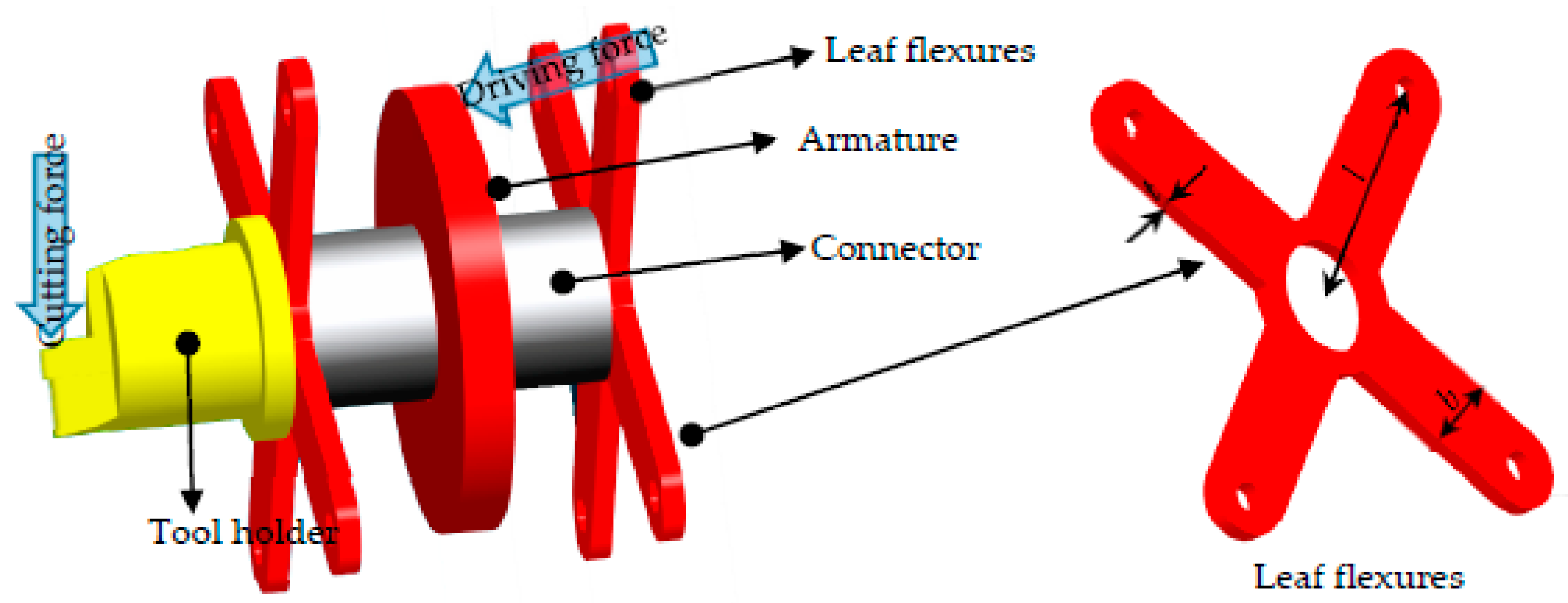
FTS systems driven by electromagnetic actuators have the potential to achieve a relatively larger stroke and higher bandwidth, but proper flexure designs play an important role in obtaining better performance. Two symmetric leaf flexures are applied in the mechanical design model in order to compensate thermal variations and mechanical disturbances. The moving part of the MEA-FTS, shown in Figure 4, consists of the armature, two symmetric leaf flexures, a connector, and a specially designed tool holder. The armature driven by the Maxwell electromagnetic force produces displacement, with flexures and the tool holder being connected to armature by the connector. The eight feet of the two flexures are fixed on the frames through bolts. When the armature is driven by the Maxwell electromagnetic force, the force passes to the flexures, resulting in elastic deformation. Following this, the displacement force is passed onto the diamond tool.
When the MEA-FTS is used for machining, the moving part of MEA-FTS will be subjected to two forces: the Maxwell electromagnetic force acting on the armature and the cutting force acting on the diamond tool. The force diagram is shown in Figure 4. In ultra-precision machining, the depth of cut is commonly very shallow (1–3 μm during the finishing cut) and thus, the cutting force (smaller than 10 N) can be neglected as being trivial compared to the driving force [18]. Thus, we ignore the effect of the cutting force during optimization of the design of the moving and electromagnetic parts of MEA-FTS in this study.
The effects of stroke, bandwidth, and rising time are determined by the mechanical stiffness. Assuming that the leaf flexures deform within the range of elastic deformation (the assumption is guaranteed through constraints) and according to Hooke’s law, the mechanical model of MEA-FTS is a cantilever structure. Therefore, the stiffness of MEA-FTS can be obtained by [19]
where E is the Young’s modulus of leaf flexures; while l, b, and t represent the length, width, and thickness of the flexure, respectively.
2.1.3. Driving Response Model
Assuming that MEA-FTS is a quadratic damping system, an equivalent kinematic model of MEA-FTS can be obtained, which is shown in Figure 5. Assuming that the damping coefficient is μ, the weight of the movement part in the system is m and according to Newton’s law, the dynamic equilibrium equation of the actuator at time t can be obtained using the equation
where z(t) is the displacement of armature at time t. Assuming that the deformation of connectors is zero, the displacement of the tool is z(t); z′′ = d2z(t)/dt2 is the acceleration of the moving part; and z′ = dz(t)/dt is the velocity of the moving part.
Following this, the transient response of the MEA-FTS can be deduced as [20]
where, ; ; and .
The first-order resonant frequency of the system can be expressed as [21]
The response time of the system can be expressed as
The response time reflects the response speed of MEA-FTS. The response time determines the controlling bandwidth if the system has a closed-loop control. The bandwidth is inversely related to the response time. Based on Equations (7) and (8), the response time td is linearly related to the reciprocal of the first-order resonant frequency f. Optimization of either will obtain the optimized bandwidth of MEA-FTS. Moreover, the first-resonant frequency should be the priority, because severe damage will occur at the first-resonant frequency. Thus, the bandwidth of the system will be measured as the first-order resonant frequency in this paper.
2.1.4. Construction and Implementation of Optimization Model
Objective Functions of the Problem
The machining characteristic of a FTS depends on its stroke and bandwidth. The stroke of a FTS determines the sagittal height of a free-form surface, while the bandwidth determines the machining speed and surface complexity. Therefore, in the optimization design, a MEA-FTS with a larger stroke and higher bandwidth would be ideal to obtain.
Substituting Equations (1) and (4) into the equations of Hooke’s law, the stroke of the MEA-FTS can be obtained by
where, r2 is the outer diameter of the armature; and r1 is the inner diameter of the armature.
According to the analysis of Section 2.1.3 and Equation (7), the first-resonant frequency of MEA-FTS can be expressed as
where, ta is the thickness of armature, ρ is the density of magnetic material.
According to Equations (9) and (10), it is concluded that stroke and bandwidth are interrelated. Furthermore, both of them are affected by dimensions of the armature and the dimensions of the designed flexure. Most of the parameters (e.g., r2, r1, t, b, l) have counter effects on the stroke and bandwidth. For example, the parameters of r2 and l should be as large as possible to obtain a larger stroke, however larger parameters of r2 and l will lead to smaller bandwidth. Thus it is impossible to obtain an FTS with large stroke and high bandwidth. There must be a trade-off between the stroke and bandwidth.
Therefore, the maximum stroke and maximum bandwidth are set as goals. In order to solve the problem easily, the objective functions are written as
where x = (x6, x5, x4, x3, x2, x1)T = (r2, r1, l, b, t, ta)are the decision variables; while F1(x) and F2(x) are continuously differentiable (highly non-linear) functions in their defined domain. All the decision variables are annotated in Figure 6.
Constraints of the Problem
In the optimization model, the variables should be solved under several constraints. These constraints are considered from several aspects as follows:
(1) Allowable stress of flexure
The kinematic model is constructed based on the elastic deformation assumption. Therefore, an inelastic deformation should be avoided. The stress constraint inequality can be expressed as
where σmax is max stress in the flexure, σlim is the allowable stress of material, and ns1 is a safety factor.
(2) Magnetic dimensional constraints
In this design, the Maxwell electromagnetic force is established under the conditions that the magnetic field in the working gaps are distributed uniformly, and the flux lines are in accord with the magnetic circuits. Assuming that the thickness of armature is ta, the constraint inequalities are
where ns2, ns3 are the safety factors; while lfr is the length of gap between the armature and permanent magnet.
(3) Dimension and processing constraints
In the mechanical design, the dimension and processing constraints should also be considered. Due to the dimensions of our sensor used for measuring the displacement of the tool holder, the inner radius of the armature should be larger than 5 mm. Thus, the constraint inequality should be (5 − r2) ≤ 0. Obviously, the outer radius of the armature should be larger than its inner radius. Thus, the constraint inequality should be (r2 − r1) ≤ 0. Due to the processing technology of the magnetic material, the outer radius of the armature should be smaller than 30 mm. Thus, the constraint inequality should be (r1 − 30) ≤ 0. Considering the processing technology and difficulty of fabrication, the thickness of flexure is restricted to being larger than 0.5 mm. Thus, the constraint inequality should be t ≥ 0.5. With the limitation for the dimensions of both the sensor and diamond turning machine, the length of flexure is restricted to be within the range of 10 mm to 50 mm. Thus, the constraint inequality should be 10 ≤ l ≤ 50.
In general, the constraint inequalities of the problem are
where G9(x) = ; G8(x) = x6 − x5 − ns3 × 10 × lfr ≤ 0; G7(x) = 5 − x5 ≤ 0; G6(x) = x6 − x5 ≤ 0; G5(x) = x6 − 30 ≤ 0; G4(x) = 0.5 − x3 ≤ 0; G3(x) = x2 − 5 ≤ 0; G2(x) = 10 − x4 ≤ 0; and G1(x) = x4 − 50 ≤ 0.
Construction of Optimization Model
In the optimization model for MEA-FTS, the stroke and bandwidth are chosen as the optimization objectives. Both the stroke and the first-resonant frequency depend on the parameters of the magnetic circuit structure, flexure structure, and dimensions of the armature [22]. The flexure dimensions (b, l, and t), the armature dimensions (r1 and r2) and the magnetic circuit dimensions (ta) are the decision variables. The optimization problem (11) can be described as
where F(x) is a continuous function mapping from 6D real space to a 2D real space; and G(x) is a continuous function mapping from a 6D real space to a 9D real space. The definition domain of the problem should be {x:|, , 2·E·x3·x23·y0≠BB·x43 }. Thus, F(x) is a non-linear continuous function, while G(x) is also a non-linear continuous function. We define f* and δ* as the expected bandwidth and stroke, respectively.
The MEA-FTS optimization problem concerns the minimization of a set of objectives while simultaneously satisfying all types of constraints. The objective function is consisted of two non-linear functions. Both are the multi-variable functions of the same parameters for MEA-FTS. The MEA-FTS optimization problem addresses the problem of reducing two non-linear functions below two goals. The design parameters of the magnetic structure and mechanical structure can be obtained. The optimization problem of MEA-FTS is a non-linear multi-objective optimization problem with several constraints. In this paper, we propose that the original problem can be solved through the SQP (sequential quadratic programming) algorithm after reformulation of the problem.
2.2. Implementation of the Problem
2.2.1. Reformulation of the Problem
In this paper, the SQP algorithm is adopted to solve the problem. The goal attainment problem formulation allows the objectives to be overachieved. Therefore, the mechanical dimensions can be relatively imprecise when related to the calculated solutions. This advantage allows for the design of mechanical structures with the consideration of limitation of equipment and processing technique [23]. Therefore, the problem is reformulated as a goal attainment problem. We define weighting ratios as W = [W1, W2], with the problem then being reformulated as
Following this, the problem can be solved using the SQP algorithm. The SQP algorithms represent in the state-of-the-art thinking in non-linear programming algorithms. This type of algorithm has superior performance in terms of efficiency, accuracy, and success [24,25]. Equation (16) concerns the minimization of a set of objectives while simultaneously satisfying all types of constraints. The objective function consists of two non-linear functions. Both are the multi-variable functions of the same parameters for MEA-FTS. The inequalities of constraints are non-linear. SQP algorithm has advantages to solve nonlinear constrained optimization problems due to the super-linear and quadratic convergence rate of sequential quadratic programming algorithm [26]. The MEA-FTS optimization problem addresses the problem of reducing two non-linear functions to stay below two goals. The design parameters of the magnetic structure and mechanical structure can be obtained. The optimization problem of MEF-FTS is a non-linear multi-objective optimization problem with several constraints. In this paper, we solve our problem using the SQP method combined with the active set technology [27].
2.2.2. Solution of the Problem
In this paper, we solve our problem using SQP method. The main idea of using SQP algorithm to solve a non-linear optimization problem is that, at each major iteration, an approximation solution is used to simplify the original non-linear problem. Following this, a new linear quadratic problem is obtained. If the optimal solution can be obtained after this, the solution is the optimal solution of the original problem. Otherwise, the new solution is used as a new approximation solution and the iteration continues until the solution of the problem is obtained [22]. Therefore, when Equation (16) is solved, a positive definite approximation of the Hessian matrix of Lagrangian should be calculated by any quasi-Newton methods such as the BFGS (Broyden, Fletcher, Goldfarb and Shanno’s Quasi-Newton) method. Then the quadratic sub-problem can be formulated as
This subproblem can be solved using the Wilson–Han–-Powell (WHP) algorithm. The solution is used to form a new iteration: (), where the step length αk should be calculated by an appropriate line search procedure so that a sufficient decrease can be obtained [25]. Following this, the solution of Equation (16) can be obtained after several iterations.
In order to solve problem (16), proper goals should be set. The stroke and bandwidth of MEA-FTS are in conflict with each other. Both of them are constrained by the power of MEA-FTS as follows
The power of MEA-FTSs are designed to be 3 kW. Based on typical applications, various goals for bandwidths and strokes are set. The solutions for each set of goals can be obtained using the SQP methods. Table 1 shows several solutions with various sets of typical goals, where f* represents the desired bandwidth; δ* represents the desired stroke; f represents the calculated value of bandwidth; and δ is the calculated value of stroke. Based on those results.
According to the solutions, it can be concluded that MEA-FTS can be applied to realize FTS with different bandwidths and strokes to complete different types of workpieces. In this paper, MEA-FTS is designed to manufacture optical free-form surfaces with brittle materials. Based on our formal processing tasks and surveys, the optimization goals with a stroke of 50 μm and a first-resonant frequency of 3.5 kHz are chosen for building our MEA-FTS. The optimized MEA-FTS can process lens-arrays on brittle materials. For example, it can process the 50 × 50 lens-arrays with an aperture of 100 mm and sagittal height of 50 μm. According to the calculation of the SQP algorithm, the MEA-FTS should have a stroke of 51.2 μm and bandwidth of 3.584 kHz. The model of the MEA-FTS with optimized parameters then can subsequently be constructed. The goal attainment problem formulation allows the objectives to be overachieved. Therefore, the mechanical dimensions can be relatively imprecise with regard to the calculated solutions. This advantage allows for designing of the mechanical structures with the consideration of limitation of equipment and processing technique.
3. Results and Discussion
3.1. Finite Element Analysis Validation
3.1.1. Finite Element Analysis for Electromagnetic Field
In order to verify the optimized results, electromagnetic finite element analysis (FEA) was employed. The electromagnetic 3-D model with optimized parameters was built. The 3-D model is rotationally symmetrical and thus, a 2-D simulation model is used in the finite element analysis, which is shown in Figure 3. Following this, the model was meshed with finite elements. NdFeB was loaded as the permanent magnet, which has an intrinsic coercivity of 1110 kA/m and a remanence flux density of 1.22 T. The exciting current was a sine wave with a frequency of 3.5 kHz and an amplitude of 160 A. Kool Mμ is chosen as the magnetic material of yokes and armature. The saturation flux density of Kool Mμ is 1.4 T, the relative permeability is 125. The boundary of this analysis is the natural boundary. The commercial software Maxwell is employed. The results can be solved.
Following this, the FEA results shown in Figure 7 can be obtained. The FEA can provide designers with the distributions of magnetic flux density and driving force. The distribution results indicated that the flux lines are consistent with the magnetic circuit designs and parameters. According to the FE analysis, the maximum driving force can be calculated as: Fmax = 2π × 35.592 = 223.63 N. The weight of the moving part is measured to be 30.71 g. This driving force can provide the FTS armature with a maximum driving acceleration of a = Fmax/m = 223.63 N/30.71 g = 305 G (G = 9.8 m/s2).
3.1.2. Finite Element Analysis for Mechanical Structure
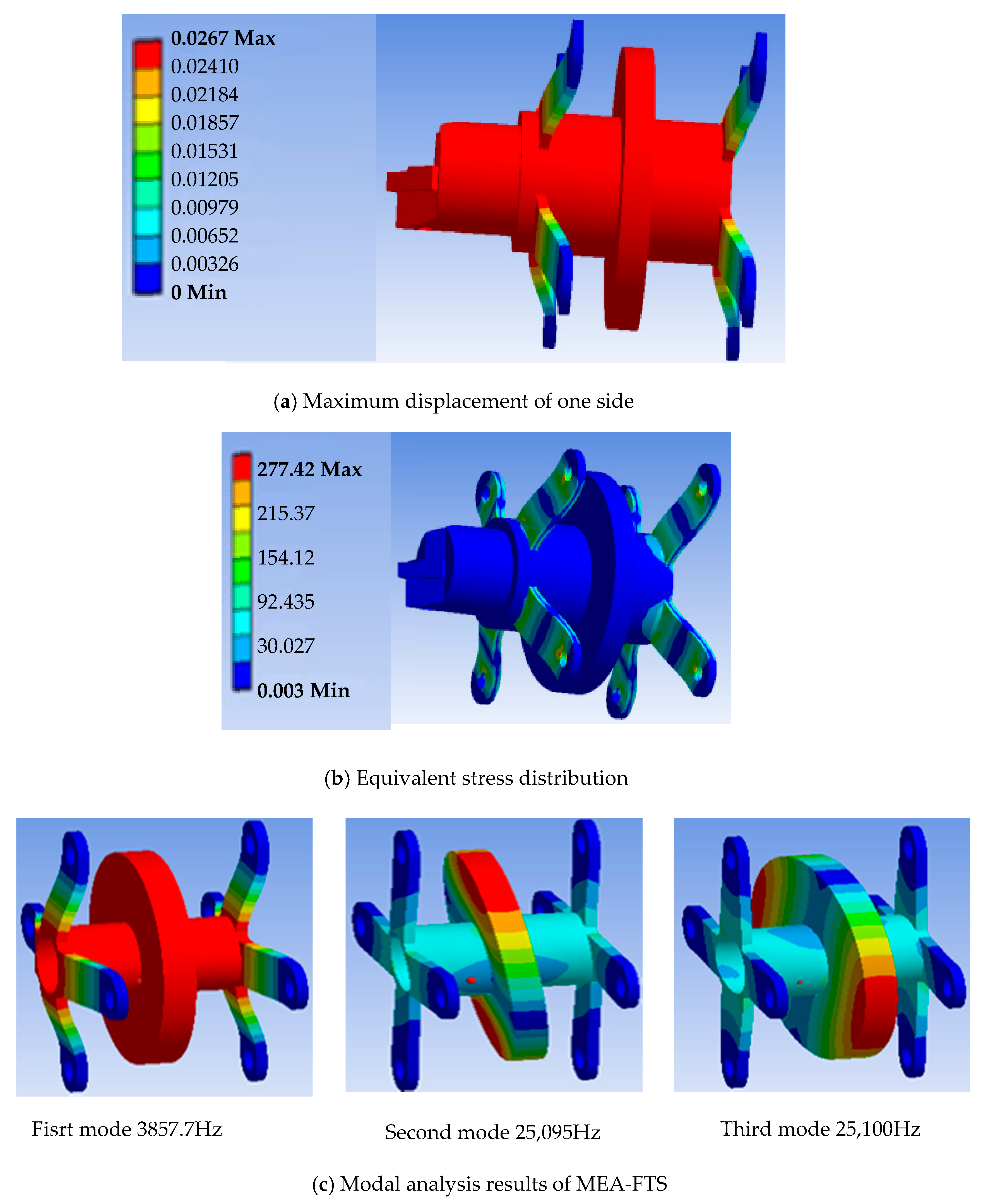
Based on the optimization results, a 3-D mechanical model was built to evaluate the stroke, stress distribution, and first-resonant frequency of the optimized MEA-FTS. The driving force which was obtained in the finite element analysis for electromagnetic field was loaded. According to the FEA results of the mechanical structure shown in Figure 8, it is concluded that: (1) the stroke of MEA-FTS is 53.4 μm as shown in Figure 8a, while the first-resonant frequency is 3.857 kHz as shown in Figure 8c. Although the value of the FEA result is slightly lower than that of the optimized result, the design objectives of the optimization can still be satisfied. It can be speculated that firstly, the compromise with processing limits on dimensions leads to a difference between the optimization results and FEA results in the designs of mechanical structures. Secondly, the parts are considered as ideal rigid points in the optimization model, while the parts are considered as thousands of finite elements in the FEA model. (2) The distribution of equivalent stress is shown in Figure 8b. Therefore, it can be concluded that the stress mainly distributes in two flexures. Furthermore, there would be a stress concentration problem in the contact region between the flexure and the fixing bolt. Considering that the maximum stress in the MEA-FTS model is 277.42 MPa, a Mn65 spring steel is chosen as the flexure material.
According to the mechanical FEA results, the optimization model is able to achieve the design goals. The MEA-FTS can achieve a stroke of up to 53.4 μm (shown in Figure 8a) and retains a bandwidth of 3.8 kHz (shown in Figure 8c) at the same time. It cannot be ignored that the second resonant frequency is 25 kHz, which is shown in Figure 8c. Thus, if a proper control method is designed, the bandwidth of MEA-FTS can be extended to about 25 kHz.
3.2. Experiment Tests
Verification experiments were carried out to validate the optimization results of MEA-FTS. The experiment was performed on a self-designed platform. The platform used for the MEA-FTS experiments is shown in Figure 9. Operational power amplifiers were used to amplify the driving current to reach a current of 160 A. The current was applied to MEA-FTS to generate displacement. The displacements were measured by a laser sensor, which has a resolution of 10 nm, measurement range of 100 µm, and a bandwidth of 100 kHz.
3.2.1. Experiment of Displacement
Experiments were carried out to measure the displacement of MEA-FTS under different driving currents. Based on the results, we can conclude that the displacement of MEA-FTS is linearly related to the driving current, as shown in Figure 10. The maximum displacement in the positive direction is 25.42 μm when the maximum positive driving current is loaded. The maximum displacement in the negative direction is 24.13 μm when the maximum negative driving current is loaded. The maximum driving current in the exciting coils is 160 A. The stroke of MEA-FTS is 49.55 µm, which is slightly smaller than the optimization results. This is because we used a rubber pad to adjust the damping ration μ, in this experiment, which was larger than expected.
3.2.2. Experiment of Frequency Response
A frequency experiment was carried out. Sine wave signals with different frequencies ranging from 0.2 Hz to 100 kHz were amplified to drive the actuator. Following this, the displacement of MEA-FTS was measured by the sensor. The frequency response experimental results are shown in Figure 11. In the results, we found that the stroke became larger after the frequency of 3.2 kHz. Therefore, the first resonant frequency (bandwidth) is 3.2 kHz. The dropping of the curve from 22 kHz is due to the bandwidth of the power amplifier.
3.2.3. Experiment of Dynamic Response
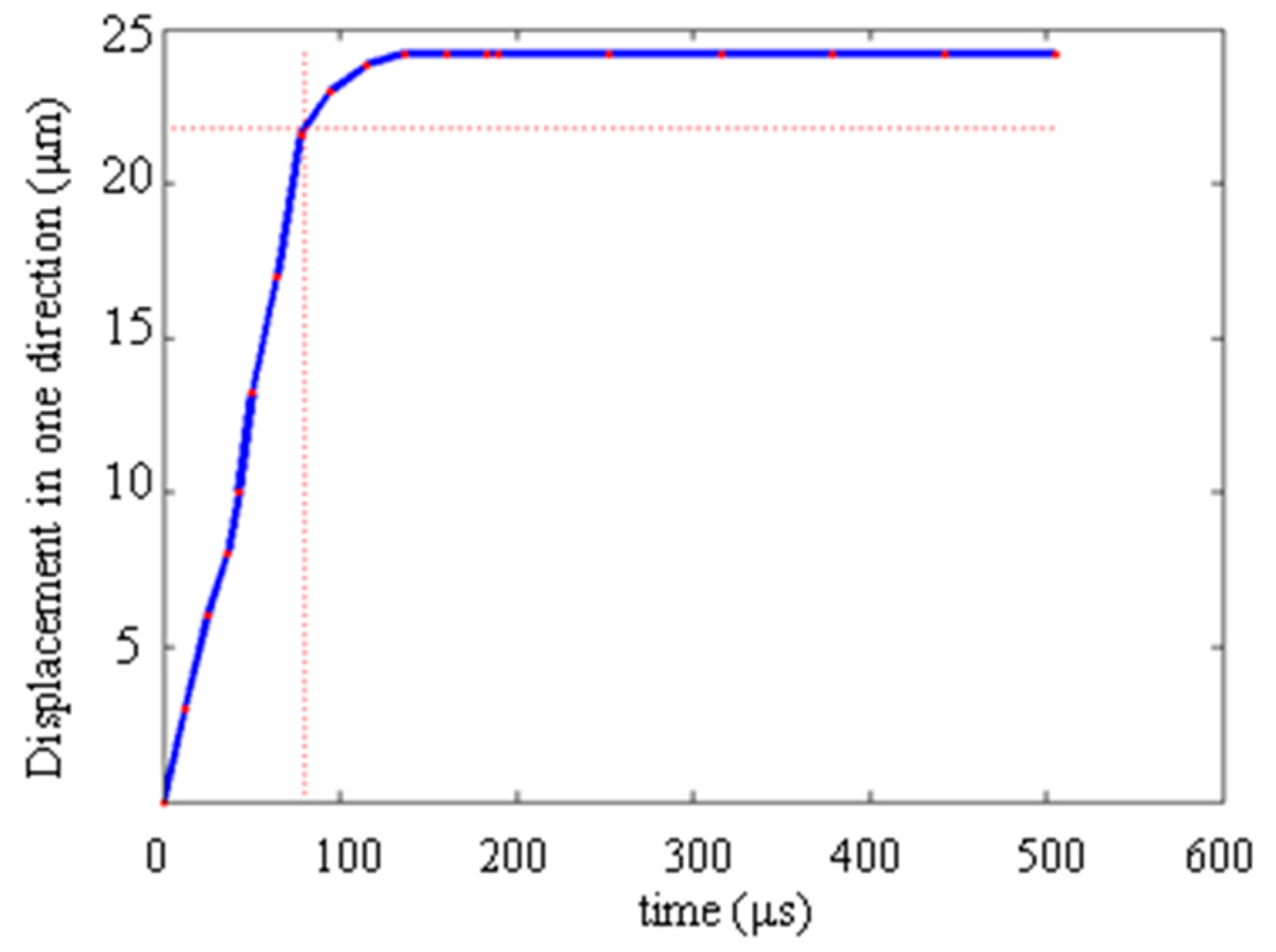
A step response test was carried out to measure dynamic characteristics of MEA-FTS. The square wave was used as the exciting signal. The experiment results are shown in Figure 12. Based on experiment results, we can conclude that: (1) MEA-FTS can be accounted as a second order elastic damping system; (2) the response time was 80.48 μs, so MEA-FTS can be driven to a maximum of 3.11 kHz with closed-loop control; and (3) MEA-FTS had no overshoot in its step response curve. Therefore, when it is applied in free-form machining applications, no over-cut problem will exist.
The optimization goals are satisfied based on the experimental results. The optimization model proposed in this paper can be used to obtain design parameters of other FTS with a selected variety of strokes and bandwidths. MEA-FTS can be applied to fabricate free-form optics.
4. Conclusions
An optimized MEA-FTS is designed in this paper. The main characteristic parameters of MEA-FTS are chosen as the optimal goals of the model. The optimization problem is built on the electromagnetic model, mechanical model, and kinematic model of the MEA-FTS system under consideration of various constraints. The original problem is reformulated as a goal attainment problem. Following this, the SQP method is introduced to solve this multi-objective non-linear optimization problem. Several sets of goals with diverse applications were solved and the design parameters of MEA-FTSs were obtained.
In order to fabricate free-form optics with brittle material, a MEA-FTS was built. Based on the optimization results, the optimized stroke and first resonant natural frequency were 51.2 μm and 3.584 kHz, respectively. Finite element analysis and experiments were conducted to verify the optimization results. The final bandwidth is 3.2 kHz and the stroke is 49.55 µm. It can be concluded that the optimization model and SQP method can be used to solve the design parameters for a MEA-FTS.
Acknowledgments
This work was supported by the Tianjin Higher Education Science and Technology Development Fund Project (No. JWK1709, JWK1716) and Tianjin Market and Quality Supervision and Management Commission of Science and Technology Project (No. 2016-W03).
Author Contributions
Yahui Nie performed the optimal design and simulations, the experiments, analyzed the results, and wrote the paper; Yinfei Du contributed with the experiments and analysis; Zhuo Xu created the MEA-FTS.
Conflicts of Interest
The authors declare no conflicts of interest. The founding sponsors had no role in the design of the study; in the collection, analyses, or interpretation of data; in the writing of the manuscript, or in the decision to publish the results.
References
- Chapman, G. Ultra-Precision Machining Systems; an Enabling Technology for Perfect Surfaces; Moore Nanotechnology Systems: Keene, NH, USA, 2004; Volume 1, pp. 1–9. [Google Scholar]
- Drive Technique Comparisons 2005. Available online: http://www.pecncsu.edu (accessed on 8 October 2011).
- Kirk, R.; Roblee, J. Freeform Machining with Precitech Servo Tool Options; Precitech Ultra Precision Technology: Berwyn, PA, USA, 2005; Volume 25, pp. 1–10. [Google Scholar]
- Physik Instrumente. Fast Tool Servo Precision Machining Piezo Actuator. Available online: http://www.pi-usa.us (accessed on 8 October 2013).
- Ma, H.Q.; Tian, J.; Hu, D.J. Development of a fast tool servo in noncircular turning and its control. Mech. Syst. Signal Process. 2013, 41, 705–713. [Google Scholar] [CrossRef]
- Kang, D.; Kim, K.; Kim, D.; Shin, J.; Gweon, D.-G.; Jeong, J. Optimal design of high precision XY-scanner with nanometer-level resolution and millimeter-level working range. Mechatronics 2009, 19, 562–570. [Google Scholar] [CrossRef]
- Zhou, X.; Hu, L. An improved adaptive feedforward cancellation for tool trajectory tracking in diamond turning of freeform optics. In Proceedings of the 2010 International Conference on Mechanic Automation and Control Engineering, Wuhan, China, 26–28 June 2010; pp. 3590–3593. [Google Scholar]
- Gutierrez, H.M.; Ro, P.I. Magnetic servo levitation by sliding-mode control of nonaffine systems with algebraic input invertibility. IEEE Trans. Ind. Electron. 2005, 52, 1449–1455. [Google Scholar] [CrossRef]
- Lu, X.D.; Trumper, D.L. Ultrafast tool servos for diamond turning. CIRP Ann. Manuf. Technol. 2005, 54, 383–388. [Google Scholar] [CrossRef]
- Zhu, Z.W.; Zhou, X.Q.; Liu, Z.W.; Wang, R.Q.; Zhu, L. Development of a piezoelectrically actuated two-degree-of-freedom fast tool servo with decoupled motions for micro-/nanomachining. Precis. Eng. 2014, 38, 809–820. [Google Scholar] [CrossRef]
- Yang, Y.; Chen, S.; Huo, D.; Cheng, K. Performance analysis and optimal design of fast tool servo used for machining microstructured surfaces. Process. Inst. Mech. Eng. Part C 2008, 222, 1541–1546. [Google Scholar] [CrossRef]
- Zhu, Z.W.; Zhou, X.Q.; Liu, Q.; Zhao, S.X. Multi-objective optimum design of fast tool servo based on improved differential evolution algorithm. J. Mech. Sci. Technol. 2011, 25, 3141–3149. [Google Scholar] [CrossRef]
- Zhuang, C.; Xu, M.; Xiong, Z. Multi-objective topology optimization of compliant mechanism for fast tool servo. In Proceedings of the IEEE/ASME International Conference on Advanced Intelligent Mechatronics (AIM), Wollongong, Australia, 9–12 July 2013. [Google Scholar]
- Rakuff, S.; Cuttino, J.F. Design and testing of a long-range, precision fast tool servo system for diamond turning. Precis. Eng. 2009, 33, 18–25. [Google Scholar] [CrossRef]
- Lu, X. Electromagnetically-Driven Ultra-Fast Tool Servos for Diamond Turning. Ph.D. Thesis, Massachusetts Institute of Technology, Cambridge, MA, USA, 2005. [Google Scholar]
- Wu, D.; Xie, X.D.; Zhou, S.Y. Design of a normal stress electromagnetic fast linear actuator. IEEE Trans. Magn. 2010, 46, 1007–1014. [Google Scholar]
- Fang, F.Z.; Nie, Y.H.; Zhang, X.D. Design of fast tool servo system based on magnetic field analysis. Nanotechnol. Precis. Eng. 2011, 9, 539–544. [Google Scholar]
- Lee, W. Prediction of microcutting force variation in ultra-precision machining. Precis. Eng. 1990, 12, 25–28. [Google Scholar] [CrossRef]
- Smith, S.T. Flexures: Elements of Elastic Mechanisms; Gordon and Breach Science Publishers: Perth, Australia, 2000. [Google Scholar]
- Nie, Y.H.; Fang, F.Z.; Zhang, X.D. System design of Maxwell force driving fast tool servos based on model analysis. Int. J. Adv. Manuf. Technol. 2014, 72, 25–32. [Google Scholar] [CrossRef]
- Franklin, G.F.; David, J.P.; Abbas, E.-N. Feedback Control of Dynamics Systems; Pretince Hall Inc.: Upper Saddle River, NJ, USA, 2006. [Google Scholar]
- Schittkowski, K.; Zillober, C.; Zotemantel, R. Numerical comparison of nonlinear programming algorithms for structural optimization. Struct. Multidiscip. Optim. 1994, 7, 1–19. [Google Scholar] [CrossRef]
- Grace, A.C.W. Computer-Aided Control System Design Using Optimization Techniques. Ph.D. Thesis, University of Wales, Bangor, Gwynedd, UK, 1989. [Google Scholar]
- Francisco, F.; Fischer, A.; Kanzow, C. On the accurate identification of active constraints. SIAM J. Optim. 1998, 9, 14–32. [Google Scholar]
- Fletcher, R.; Leyffer, S.; Ralph, D.; Scholtes, S. Local convergence of SQP methods for mathematical programs with equilibrium constraints. SIAM J. Optim. 2006, 17, 259–286. [Google Scholar] [CrossRef]
- Luo, Z. The Study of Sequential Quadratic Programming (SQP) Algorithms. Ph.D. Thesis, Guilin University of Electronic Technology, Guilin, China, 2008. [Google Scholar]
- Hu, Q. Research on Sequential Quadratics Programming Method for Solving Constrained Optimization. Ph.D. Thesis, Hunan University, Hunan, China, 2008. [Google Scholar]
Figure 1.
The stroke and bandwidth characteristics of a series of FTS.
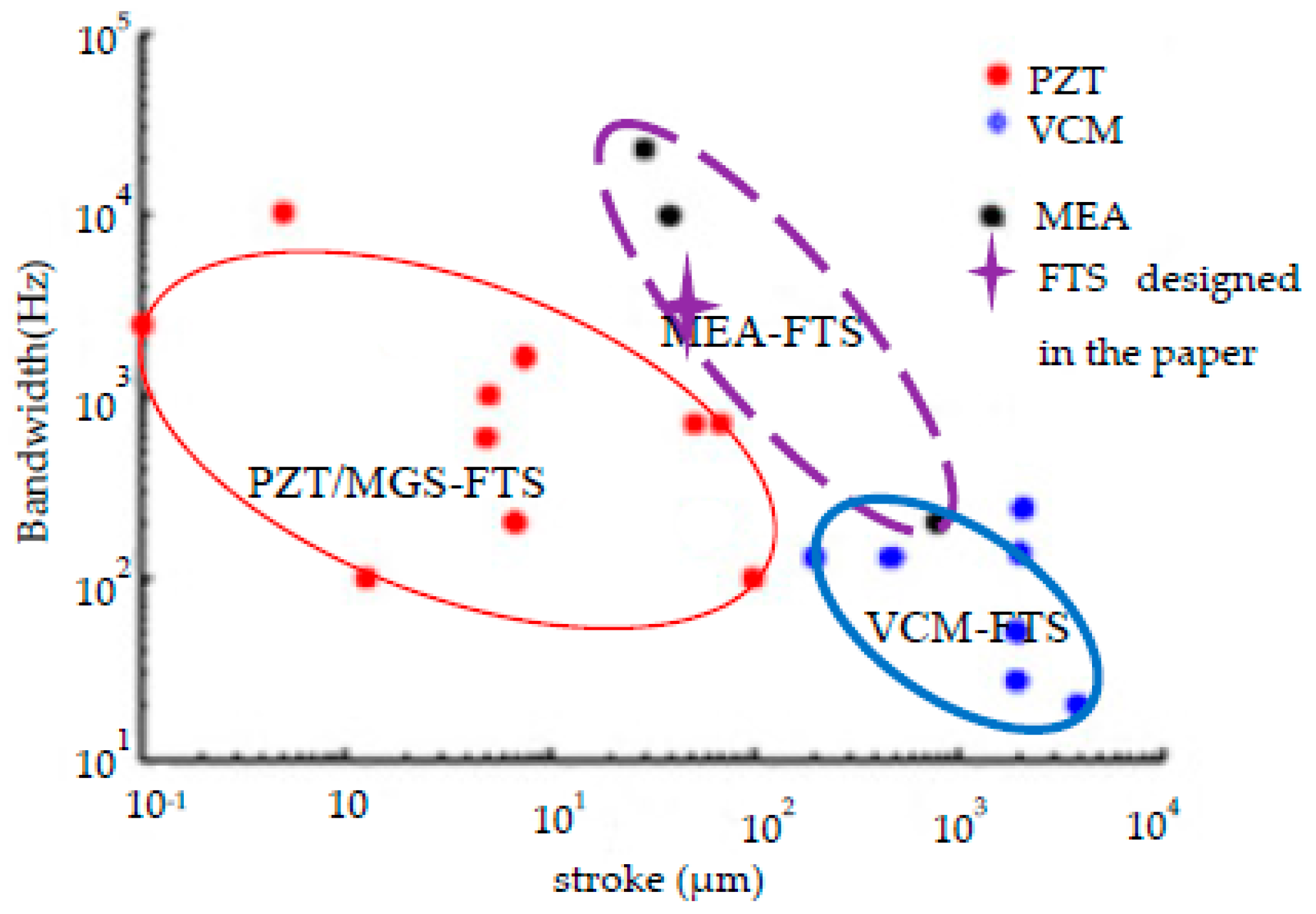
Figure 2.
3D model of MEA-FTS.

Figure 3.
2D model of the magnetic part.
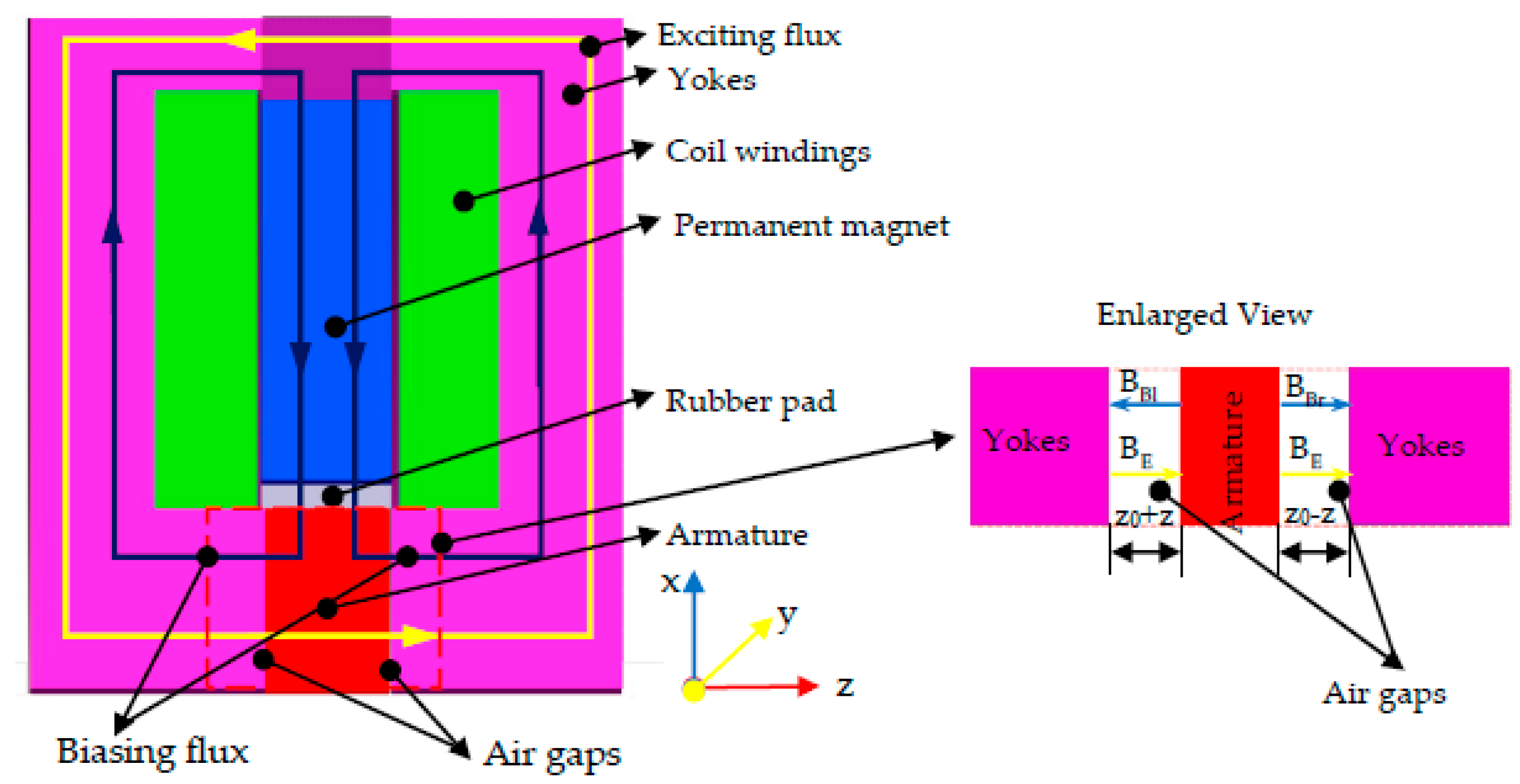
Figure 4.
Moving part of MEA-FTS.

Figure 5.
Equivalent kinematic model of MEA-FTS.
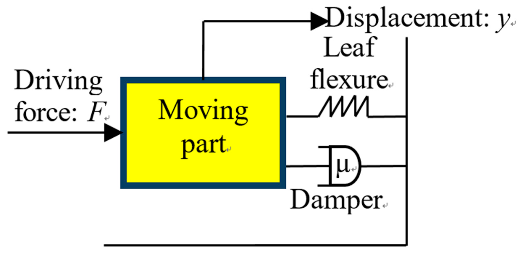
Figure 6.
Annotation of decision variables.
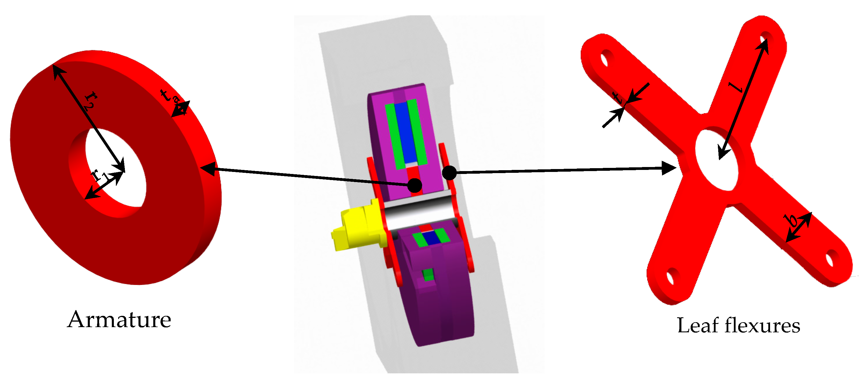
Figure 7.
Magnetic flux lines in the MEA-FTS model.
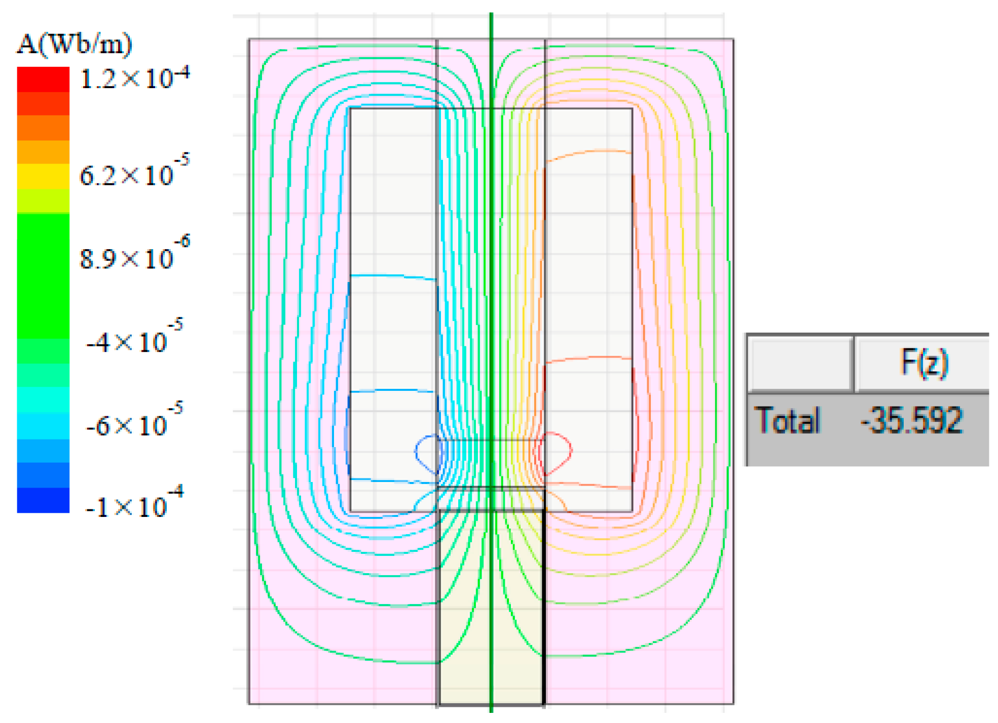
Figure 8.
Mechanical FEA results.

Figure 9.
The experiment platform of MEA-FTS.
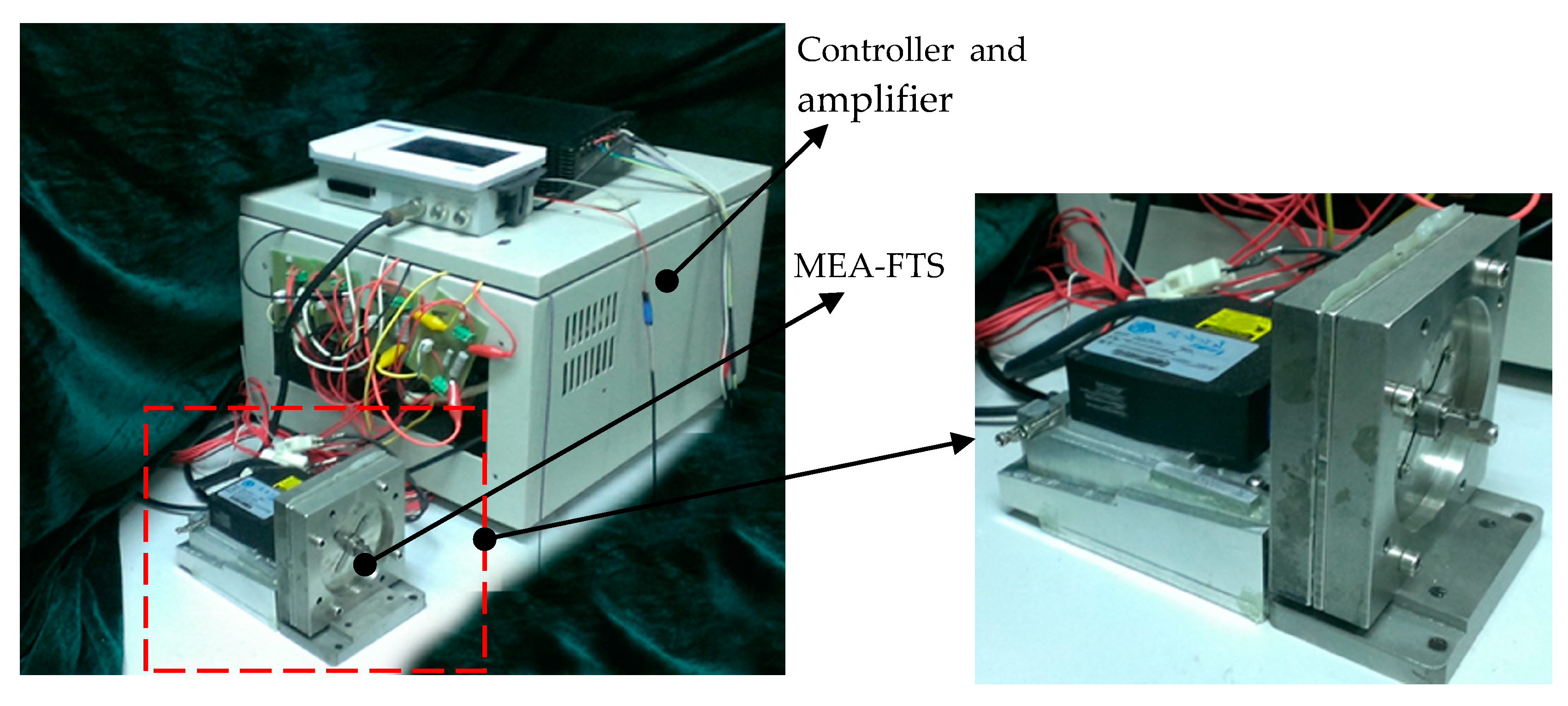
Figure 10.
The displacement of MEA-FTS under different driving currents.
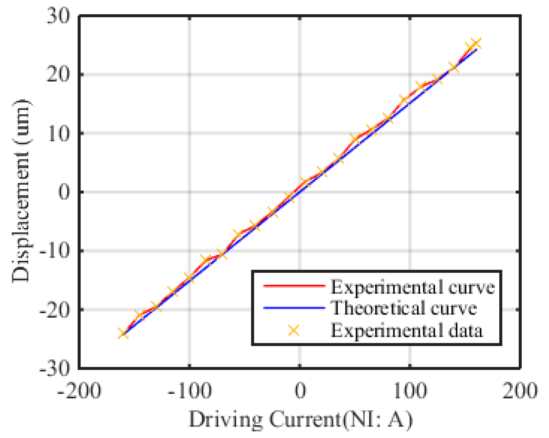
Figure 11.
Frequency response curve of MEA-FTS.
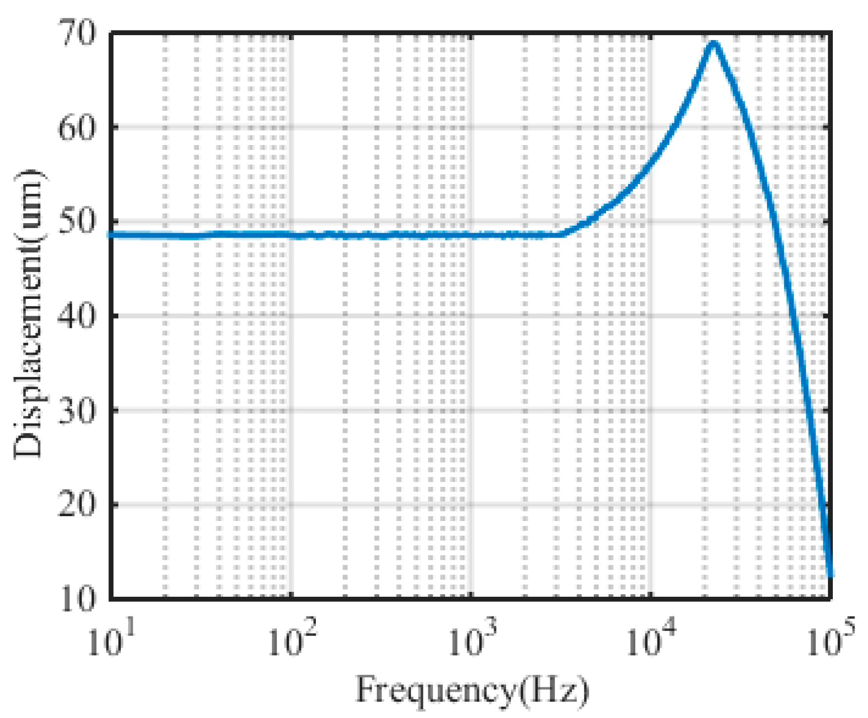
Figure 12.
The step response curve of MEA-FTS.


Table 1.
Solutions with various sets of typical goals.
| f* (Hz) | δ* (μm) | f (Hz) | δ (μm) | t (mm) | b (mm) | l (mm) | r1 (mm) | r2 (mm) |
|---|---|---|---|---|---|---|---|---|
| target bandwidth | target stroke | optimized bandwidth | optimized stroke | optimized thickness of flexure | optimized width of flexure | optimized length of flexure | optimized outer radius of armature | optimized inner radius of armature |
| 500 | 250 | 786.9 | 127.6 | 1.4 | 9.8 | 17.8 | 3.5 | 14.9 |
| 1000 | 100 | 999.4 | 99.4 | 1.1 | 4.5 | 10 | 3.8 | 15 |
| 2000 | 50 | 1.969 k | 49.2 | 1.4 | 5.4 | 10 | 5 | 15 |
| 3000 | 30 | 3.057 k | 30.57 | 1.5 | 6.1 | 10 | 5 | 15 |
| 3500 | 25 | 3.584 k | 25.6 | 1.6 | 6.4 | 10 | 5 | 15 |
| 5000 | 18 | 4.925 k | 17.73 | 1.7 | 7 | 10 | 5 | 15 |
© 2017 by the authors. Licensee MDPI, Basel, Switzerland. This article is an open access article distributed under the terms and conditions of the Creative Commons Attribution (CC BY) license (http://creativecommons.org/licenses/by/4.0/).
Share and Cite
MDPI and ACS Style
Nie, Y.; Du, Y.; Xu, Z. Optimization Design of Electromagnetic Actuator Applied as Fast Tool Servo. Actuators 2017, 6, 25. https://doi.org/10.3390/act6030025
AMA Style
Nie Y, Du Y, Xu Z. Optimization Design of Electromagnetic Actuator Applied as Fast Tool Servo. Actuators. 2017; 6(3):25. https://doi.org/10.3390/act6030025
Chicago/Turabian StyleNie, Yahui, Yinfei Du, and Zhuo Xu. 2017. "Optimization Design of Electromagnetic Actuator Applied as Fast Tool Servo" Actuators 6, no. 3: 25. https://doi.org/10.3390/act6030025
Note that from the first issue of 2016, this journal uses article numbers instead of page numbers. See further details here.