Piezoelectric Motor Using In-Plane Orthogonal Resonance Modes of an Octagonal Plate

Physik Instrumente GmbH & Co. KG, Auf der Roemerstrasse, 1, 76228 Karlsruhe, Germany
*
Author to whom correspondence should be addressed.
Actuators 2018, 7(1), 2; https://doi.org/10.3390/act7010002
Submission received: 26 September 2017
/
Revised: 1 December 2017
/
Accepted: 4 December 2017
/
Published: 6 January 2018
(This article belongs to the Special Issue Electrochemical and Electromechanical Actuators)
Abstract
:Piezoelectric motors use the inverse piezoelectric effect, where microscopically small periodical displacements are transferred to continuous or stepping rotary or linear movements through frictional coupling between a displacement generator (stator) and a moving (slider) element. Although many piezoelectric motor designs have various drive and operating principles, microscopic displacements at the interface of a stator and a slider can have two components: tangential and normal. The displacement in the tangential direction has a corresponding force working against the friction force. The function of the displacement in the normal direction is to increase or decrease friction force between a stator and a slider. Simply, the generated force alters the friction force due to a displacement in the normal direction, and the force creates movement due to a displacement in the tangential direction. In this paper, we first describe how the two types of microscopic tangential and normal displacements at the interface are combined in the structures of different piezoelectric motors. We then present a new resonance-drive type piezoelectric motor, where an octagonal plate, with two eyelets in the middle of the two main surfaces, is used as the stator. Metallization electrodes divide top and bottom surfaces into two equal regions orthogonally, and the two driving signals are applied between the surfaces of the top and the bottom electrodes. By controlling the magnitude, frequency and phase shift of the driving signals, microscopic tangential and normal displacements in almost any form can be generated. Independently controlled microscopic tangential and normal displacements at the interface of the stator and the slider make the motor have lower speed–control input (driving voltage) nonlinearity. A test linear motor was built by using an octagonal piezoelectric plate. It has a length of 25.0 mm (the distance between any of two parallel side surfaces) and a thickness of 3.0 mm, which can produce an output force of 20 N.
1. Introduction
Piezoelectric motors are the main candidates for use in small mechanical systems [1,2,3,4,5,6,7,8,9,10,11,12,13,14,15,16]. The advantages compared to electromagnetic ones with the same size and weight include high power density, insensitivity towards a magnetic field, silent, direct drive without a gear mechanism, a quick response without backlash, maintaining a position with no energy consumption and a high dynamic range of velocity with high positioning accuracy [12,13,14,15,16]. According to functional principles, construction, and drive specifications, piezoelectric motors can be categorized into three groups: piezo-walk-drive, inertia-drive and resonance-drive [6].
1.1. Piezo-Walk-Drive
In a piezo-walk-drive mechanism, there are at least two sets of actuator arrangements embedded in the structure and they operate one after the other. The main reason that these motors are called piezo-walk-drive is because the moving sequences in these motors resemble two or four feed walking actions. In these motors, a step motion is realized in two ways.
In one way, there are normal and tangential microscopic displacements to the moving direction of a sliding element. Each actuator in a motor that generates a microscopic displacement has one single task, which is either to perform a “clamp” or “move” action. If an actuator has the task of performing a “clamp” action, the displacement is normal to the slider moving direction and the ultimate function of these actuators is to increase or decrease normal force and thus, to hold friction force. If an actuator is required to perform a “move” action, the displacement generated by the actuator is tangential to the moving direction of the sliding element. Expansion and shrinkage of this actuator creates a microscopic movement of the slider. After the structure proposed by Brisbane in 1965 [17], some other structures operated on the basis of the piezo-walk-drive principal [18,19,20,21]. Typically, these structures consist of three actuators, where two of them are responsible for the clamping and one is responsible for the moving action. In these motors, the required displacements in the normal and tangential directions, with respect to a sliding element, can be generated by actuators that use longitudinal, shear, transverse, and planar coupling of piezoelectric materials. In the early structures, the piezoelectric elements used in the piezo-drive type motors were in bulk forms, but in many of the commercialized structures, the actuators are manufactured in multilayer forms to generate sufficient displacement at a relatively low-driving voltage.
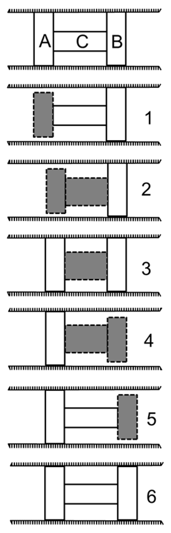
Assuming that the activation makes the length, or the diameter, decrease and release, which causes an actuator to return to its rest position, the motion sequence as seen in Figure 1 can be started by activating one clamping actuator (A). When the moving actuator (C) is also activated, shrinkage of the moving actuator generates a half step. At this moment, the clamping actuator (A) is released so that it can clamp and maintain the holding force. In the following step, the second clamping actuator (B) is activated and the moving actuator (C) is released. When the second clamping actuator (B) is released, one motion sequence is finished.
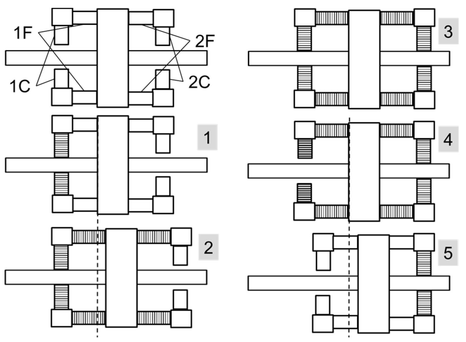
Later, we can see examples where clamping actuators are attached to the end of feeding actuators, where at least two identical sets are used in each motor structure [22]. Assuming that the activation makes the length of an actuator increase and release, making an actuator return to its rest position, motion sequence of the piezo-walk-drive, as seen in Figure 2, can be started by activating clamping actuators (1C) in the first set (step 1). A half step can be made when the moving actuators in the first and in the second set (1F and 2F) are activated (step 2). At this moment, a pushing force is generated by the moving actuators (1F) in the first set. When the clamping actuators (2C) in the second set are activated (step 3), all moving and clamping actuators are in an active state. The second half of the step is started by releasing the clamping actuators (1C) in the first set (step 4). After the moving actuators (1F and 2F) in the first and in the second sets are released (step 5), the second half of the step is completed. A new sequence can be started by activating clamping actuators (1C) in the first set, and releasing the clamping actuators (2C) in the second set. In order to obtain smoother motion, or for the purpose of better controllability, an overlap of activation and deactivation timings is possible for both clamping and moving actuators [19,20].
In other types of structures, two sets of actuators placed next to each other make “clamp-push and release” actions in sequence [23,24]. All actuators in the structure are required to perform “clamp-push and release” actions. “Clamp-push and release” actions can be fulfilled if motion generated by an actuator has an oblique or elliptical trajectory. Oblique or elliptical trajectory is generated because each actuator is electrically divided into two sections in the longitudinal direction so driving signals cause the actuator to elongate and deflect at the same time. Both actuator sets (a pair) perform a “clamp-push and release” action one after the other, with a time delay or a phase shift in the same period cycle.
Motion sequence is started by activating one set. This activation makes the moving element clamp due to elongation, and motion is created due to deflection. At the moment when the other set is initially activated, the actuator set in clamp position is then deactivated. Because the second set has been activated, the first actuator set deactivates. During this time, the sliding element does not move back, but rather advances another step.
1.2. Inertia-Drive
In inertia-drive piezoelectric motors, only the tangential component of the back-and-forth movement, at the interface between a slider and a stator within one period, generates a movement. In one direction of the tangential movement, the stator element is activated slowly. During this activation time, the inertia force acting on the slider is smaller than the friction force; the slider sticks to the contact area of the stator and moves with it. In the opposite direction of the tangential movement, the stator is deactivated faster, relative to its initial position. During this time, the inertia force acting on the slider is greater than the friction force, so the slider slips and stays behind the contact area of the stator element. At the end of one cycle, the sliding element makes a microscopic step. The accumulation of these microscopic steps creates macroscopic movement.
Deformation of the piezoelectric element in various modes, such as longitudinal, transverse or shear, is either directly transferred to a moving element or through a coupling element, where the motion generated by the piezoelectric element is converted into a tangential direction at the interface. Depending on the structure, while converting a deformation into tangential motion, a leverage mechanism could amplify the deformation. The amplified deformation could also have a normal component [25,26]. Nevertheless, having a normal component at the interface could make a motor have direction-dependent performance parameters, such as generated force and velocity, which should be compensated with magnitude and timing of a driving signal.
In inertia-drive motors, tangential movement can be generated on a slider or on a stator depending on where a piezoelectric element is embedded. If a piezoelectric element is embedded into the moving element, the motor can be considered a moving actuator type. If the piezoelectric element is embedded into the stator, the motor can be considered a fixed actuator type.
Even if there are some structures that could be considered as inertia-drive piezoelectric motors [27,28], the first practical inertia-drive (stick-slip) structure was proposed by Pohl in 1986 [29], where a piezoelectric cylinder is embedded into a four-bar mechanism (Figure 3). One side of the four-bar was attached to a base and a sliding mass is attached to the parallel bar. When the actuator is driven with a saw-tooth waveform signal, the attached mass (m) moves together with the bar. This occurs during the slow expansion period of the saw-tooth signal (sticking). This is left behind during the fast contraction period of the signal (slipping). Repeating the cyclic movements makes the attached mass move continuously. When the electric field makes the piezoelectric element expand quickly and contract slowly, the attached mass moves in the opposite direction. This mechanism was applied to precise multi-degree motion positioning device applications for an atomic force microscope. Because the piezoelectric element is embedded into the stator structure, this motor could be considered as a fixed actuator type.
In a structure proposed by Higuchi in 1986 [30], a moving mass (m1) and a weight (m2) are attached to both ends of a piezoelectric element. The whole structure is placed on a base plate and held by frictional force acting between the base plate and the moving mass (Figure 4). When an electric field is applied to the piezoelectric element, rapid expansion of the piezoelectric element creates an acceleration, causing the moving mass to overcome the static friction (slip) so both masses move in opposite directions. During the slow contraction time of the piezoelectric element, the acceleration on the moving mass cannot overcome the static friction, so only the weight moves (stick). At the end of one motion cycle, a microscopic movement is obtained. Because the piezoelectric element is embedded into the moving element, this motor could be considered as a moving actuator type. Many of the inertia-drive type motors developed afterwards operate according to the above-mentioned initial structures [31,32,33,34,35,36,37,38,39,40,41,42,43,44,45]. We can also find literature that proposes ideal driving signals with detailed analysis of motion at the interface [46,47].
1.3. Resonance-Drive
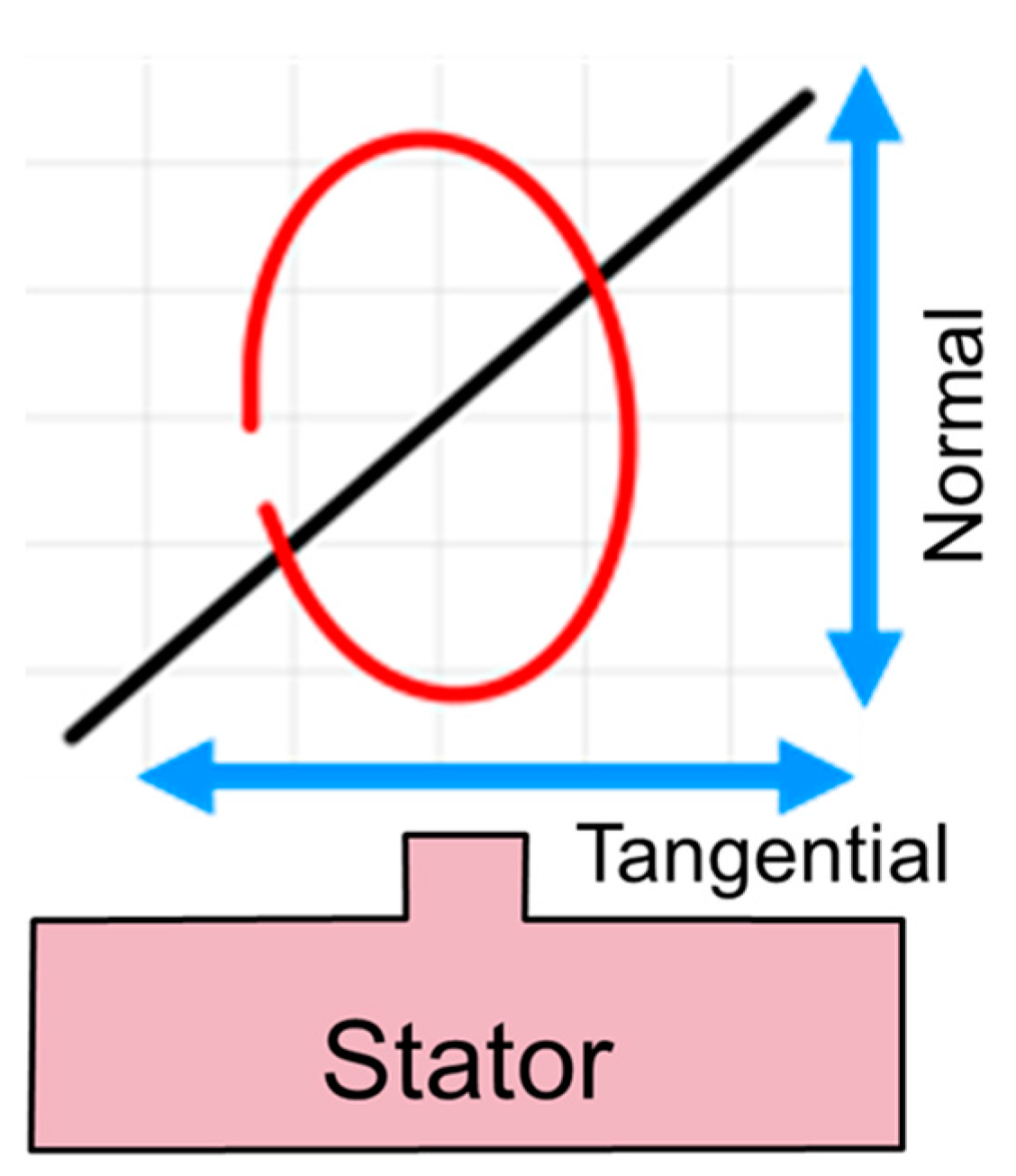
In a resonance-drive piezoelectric motor, there are two types of microscopic motions: oblique and elliptical (Figure 5). Excitation of a single mode on a vibrator is enough for generating an oblique motion. Because oblique motion can have components in the tangential and normal directions, a net microscopic motion is obtained when a stator contact point touches a rotor or a slider contact point. On the other hand, excitations of two orthogonal modes are needed for generating an elliptical motion. In a multi-mode excitation piezoelectric ultrasonic motor, there is elliptical movement at the interface, which means that there are movements in two orthogonal directions at the contact point and phase shift between these movements causes the trajectory to be elliptical at the contact point. This elliptical trajectory causes the sliding element to perform microscopic motion in every cycle.
Among the piezoelectric motors, resonance-drive (or ultrasonic) motors were the actuators that were studied the most. The first idea of converting electrical oscillation into mechanical movement dates back to 1927 [48], and we can see various attempts to obtain longer, mechanical motion using the inverse piezoelectric effect [49,50,51,52,53,54,55]. We have classified resonance-drive piezoelectric motors based on various criteria such as, type of microscopic motion at the interface, and the method of direction change. The interested reader can refer to our previous paper [6].
In literature, we can see piezoelectric motors operated at resonance [56,57,58,59,60], where the generated modes are not in orthogonal directions. Because the generated movement at the contact point is in the tangential direction, these motors should be considered as inertia-drive types. There are also piezo-walk-drive motors that are operated at resonance [61,62].
In the following section, we introduce a newly developed resonance-drive type piezoelectric motor structure, where the excited microscopic movements at the interface are defined by parameters such as the frequency, magnitude and phase shift of the driving signals, and not mechanical dimensions, or resonance modes of a vibrator. With these parameters, not only oblique or elliptical, but more complex microscopic movements at the interface are also possible.
2. Structure of the Vibrator and Motor Operating Principle
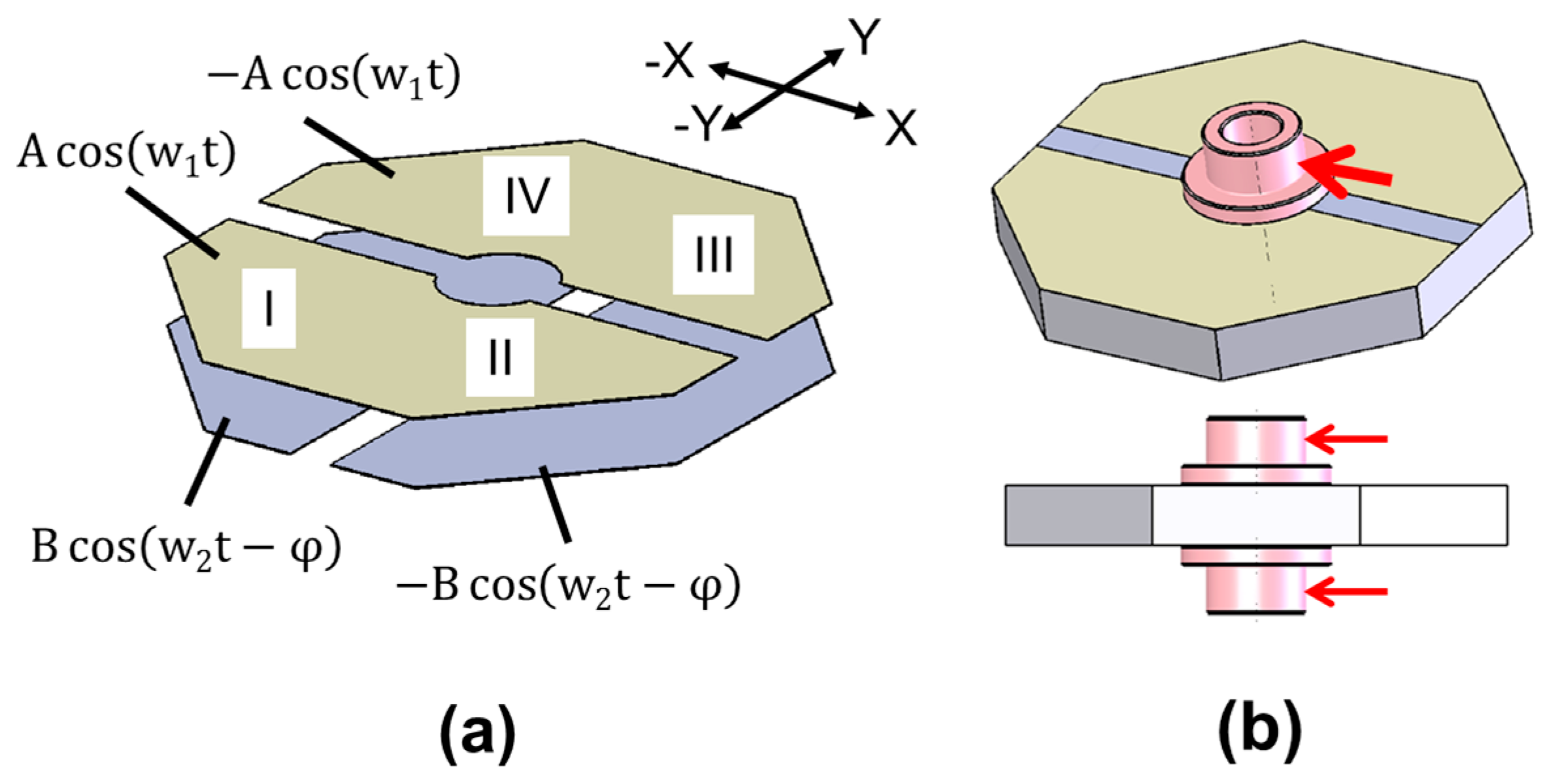
A resonance-drive type piezoelectric motor is an octagonal piezoelectric plate, which has a thickness of 3.0 mm and a length (the distance between any of the two parallel side surfaces) of 25 mm. This was introduced and is used as the stator of the motor [63]. Metal electrodes divide the main surfaces of the plate into two equal regions. The electrodes on one main surface are arranged perpendicular to the electrodes on the other main surface (Figure 6a). Two alumina eyelets, used as the friction contact elements, are attached symmetrically at the center of the top and bottom surfaces (Figure 6b).
The driving signals on the stator are applied between the two surface electrodes on both faces. When a signal is applied between the two top electrodes, we can assume that one electrode has and the other has signals. Similarly, a second signal is applied between the two bottom electrodes, when one bottom electrode has , and the other has signals (Figure 6a). Even if the applied signals are between the two surface electrodes, the resulting electric fields are between the top and the bottom electrodes in the thickness direction. Assuming that the thickness of the octagonal plate is d, we can write the electric field for the four quarter regions as follows.
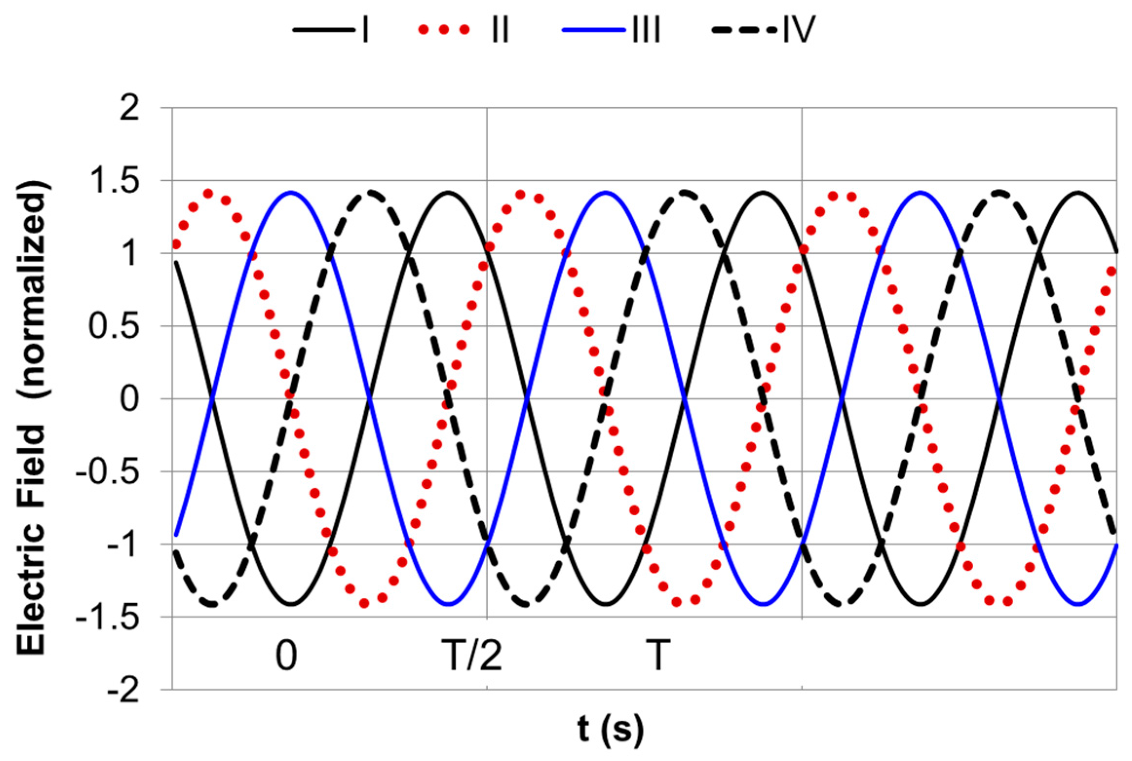
When the magnitudes A, B and thickness d are normalized to 1, the frequencies ( and ) of the signals on the top and on the bottom electrodes are equal and the phase angle () is set to 9 degrees. Because of the “sum to product trigonometric identity”, the electric field equations can be rewritten as:
Since , the magnitude of the normalized electric fields are , which means that the plate is exposed to a 42% higher electric field. Moreover, the phase difference of the normalized electric field between any of the two adjacent regions is still 90 degrees (Figure 7).
When the phase shift () is 0 degrees, one can easily find that section I and III have zero electric fields, but the magnitude of the normalized electric field in section II and IV is 2. Similarly, when phase shift () is 180 degrees, section II and IV have zero electric fields and the magnitude of the normalized electric field in section I and III is zero. For phase shift () of other values, the electric fields in these regions change accordingly.
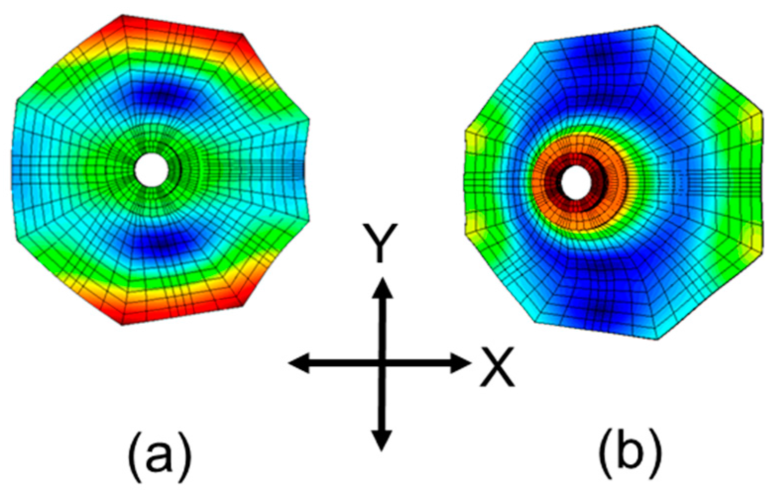
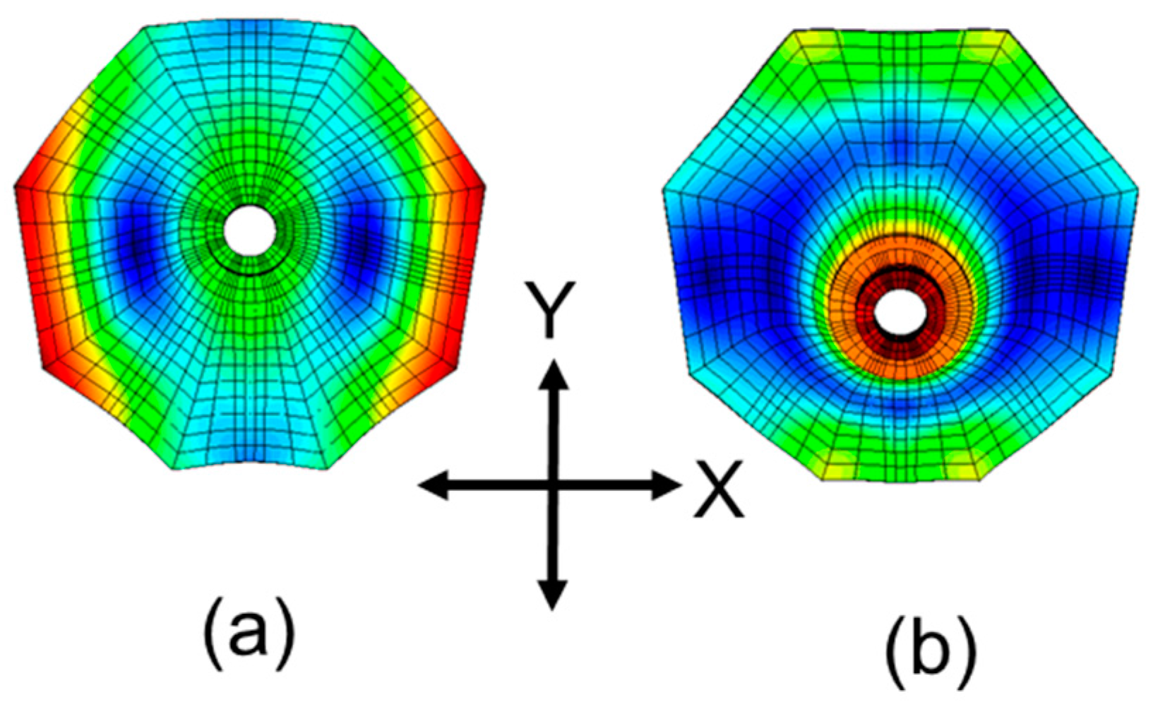
When only the bottom electrodes are excited with the signals ( and ), leaving the top electrodes floating, the in-plane modes are excited only in the x-axis direction (note that frequencies of the signals between the top and bottom electrodes are assumed to be the same). The corresponding first and second in-plane mode shapes, which were calculated by using ATILA-GID software (ATILA-GID 2.0.0, Micromechatronics Inc, State College, PA, USA), are shown in Figure 8. When the signals ( and ) are applied in between the two top electrodes, only the modes in the y-axis direction are excited. The corresponding first and second in-plane mode shapes in the y-axis direction are shown in Figure 9. Because the electrodes on the main surfaces are identical but orthogonal, the excited in-plane modes are also identical but orthogonal. When the driving signals are applied at the same time by setting the phase shift () to 90 degrees, the resulting movement is nothing but a hula-hoop trajectory. Indeed, the microscopic movement on the surface of the center eyelets can be controlled fully by configuring the magnitude and phase shift of the top and the bottom signals.
When the magnitudes (A and B) at the top and the bottom signals are set to 1 V, the calculated displacements are seen in Figure 10. These displacements were calculated using ATILA-GID software, on the side of the eyelet at the first in-plane resonance mode (at 68.7 kHz), and at the second in-plane resonance mode (at 154.5 kHz). Magnitude of the displacement under the same electric fields at the second in-plane resonance mode is larger than the displacement at the first in-plane mode. This result is expected because maximum displacement, as seen in Figure 8 and Figure 9 at the first in-plane resonance, is at the side surface of the octagonal plate.
Movement trajectories on the side of the eyelet at 68.7 kHz for three driving conditions are seen in Figure 11. At this frequency, the displacement generated on the side surface of the coupling elements (eyelets) is circular. When the magnitude of the signal applied on the top and on the bottom electrodes is the same (A = B = 1 V) and the phase shift (φ) between the two signals is 90 degrees, the trajectory is a circle. When the magnitude of the applied signal in between the top electrodes is doubled (in this case: A = 2 V, B = 1 V), only the magnitude of the displacement in the y-axis direction is doubled. Similarly, When the magnitude of the applied signal between the bottom electrodes is doubled (in this case: A = 1 V, B = 2 V), only the magnitude of the displacement in the x-axis direction is doubled.
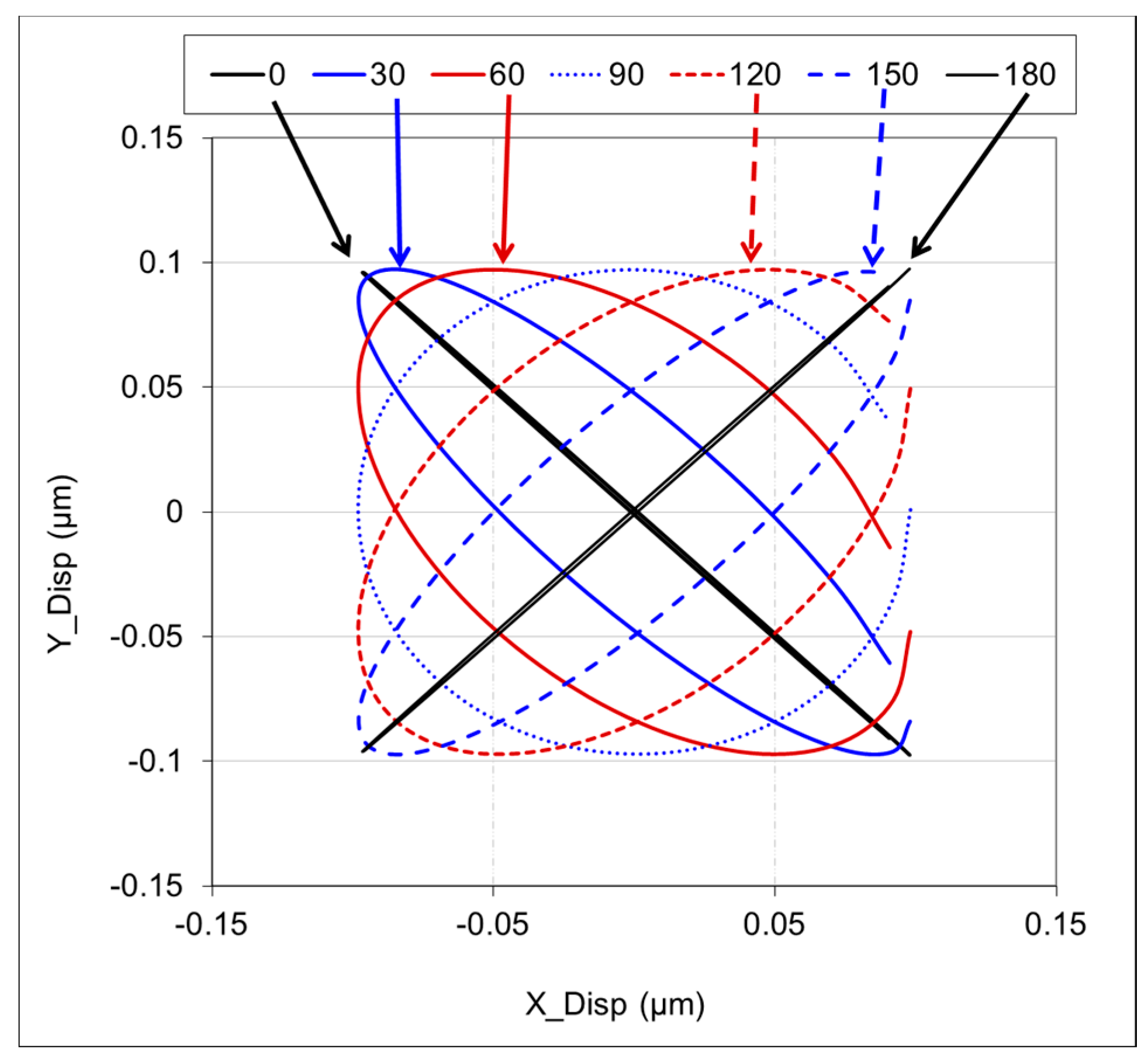
When the phase angle (φ) between the signals on the top and on the bottom electrodes is changed from 0 to 180 degrees by setting the magnitudes (A and B) to 1 V, the shape of the elliptical motion also changes (Figure 12). Note that when the phase angle is 0 degrees, the motion is in the oblique direction. This is because there are electric fields only in the two diagonal regions (II and IV as marked in Figure 6). In the other two diagonal areas (regions I and III), the electric fields are zero. When the phase angle is 180 degrees, the motion is again in the oblique direction. In this case, there are electric fields only in the two diagonal regions (I and III), and the other two diagonal regions (II and IV) have zero electric field.
2.1. Structure of the Linear Motor
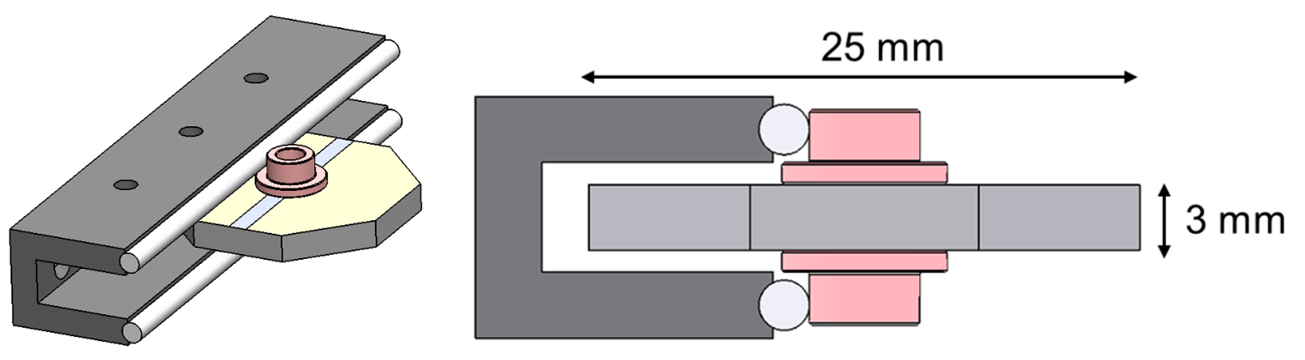
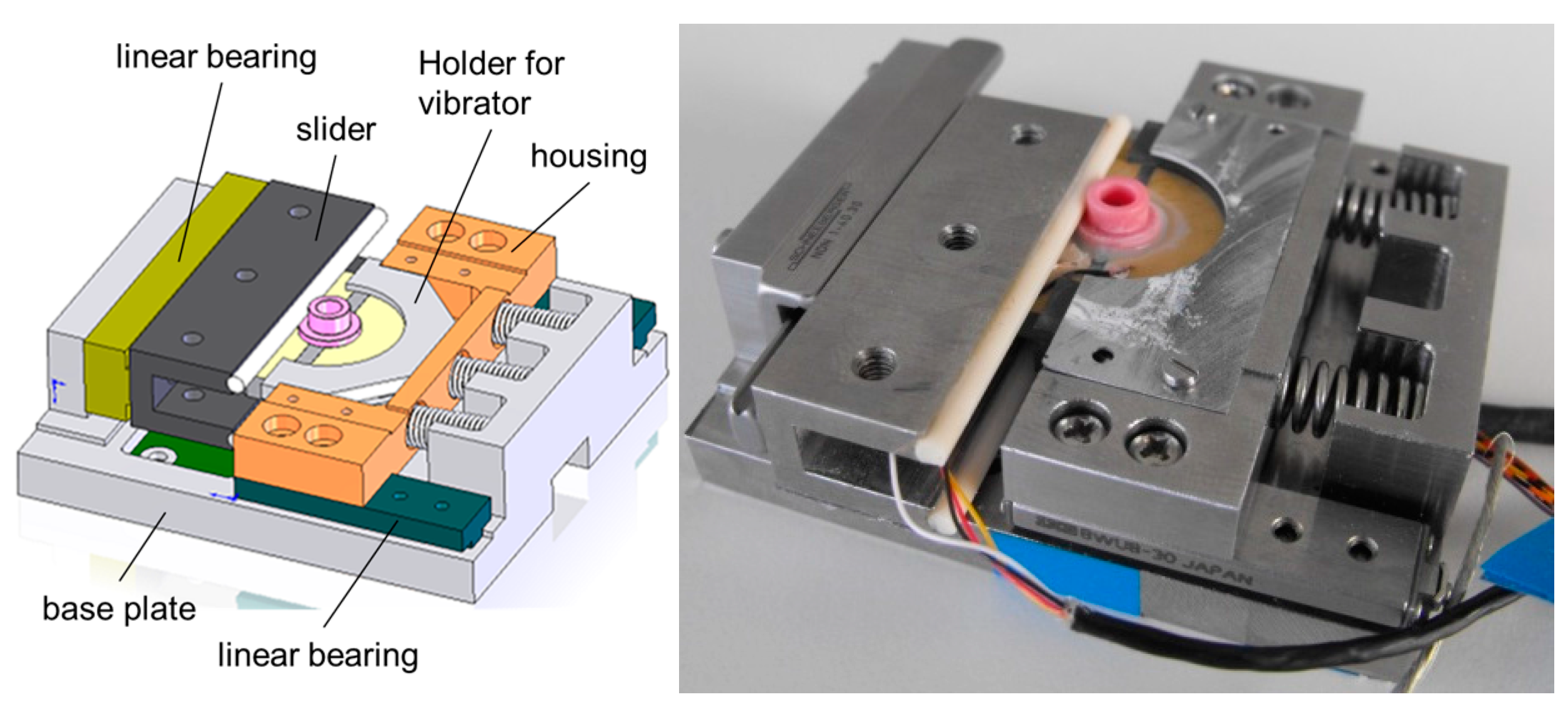
In the test motor, the piezoelectric vibrating element was placed between two identical plastic holders made from PEEK material and placed together in a steel housing. The steel housing was guided by two linear bearings in the pre-stress direction. The two linear bearings were fixed on a base plate. A slider that has a U-shaped cross-section guided by another larger linear bearing was also fixed on the base plate. Two alumina rods were attached to both ends of the U-shaped slider. The side surfaces of the two eyelets on the vibrator and the two alumina rods on the slider were in contact tangentially (Figure 13). Two or three springs applied pressure against the slider. In the test motor, a position sensor was embedded in the base plate and a reflective surface was attached to the side surface of the U-shaped slider (Figure 14).
Two phase sinusoidal waveform signals with independent magnitude and phase shift were generated by a “Multifunction Synthesizer” (WF1946B, NF Corp., Yokohama, Japan) and amplified by two power amplifiers (HAS 4011 and HAS4014, NF Corp.). Before applying the two signals to the test motor, two electromagnetic transformers, with their primary and secondary side turn ratio of 1:1, were used to shift the common grounds to a floating state. In this case, when the signal on one of the top electrodes was , the other signal on the other top electrode would be ). Magnitudes of these signals control the displacement in the normal direction. The second signal, with a phase shift of 90 degrees from the other power amplifier, was also applied first to an electromagnetic transformer and applied to bottom electrodes. The signals on the bottom electrodes ( and ) control displacement in the tangential direction.
The slider position data were collected by a PC. The position data collected were used to calculate the motor control input and speed, and load characteristics.
2.2. Speed Characteristics
Conventionally, the speed of an ultrasonic motor for one- or two-phase driving type resonance piezoelectric motors is controlled by changing the magnitude of the driving signals, or the phase difference between the two signals, which results in microscopic movements in the normal and tangential directions at the interface, to increase or decrease at the same time. The disadvantage of both driving methods is nonlinearity, such as dead-zone and hysteresis, especially in the low-speed region. In this motor, microscopic motion at the contact points in the tangential and normal directions is generated by the driving signals on the top and on the bottom electrodes, respectively. When the corresponding electrodes that are responsible for generating tangential displacements are excited, displacement is generated only in a tangential direction. Similarly, when the corresponding electrodes that are responsible for generating normal displacements are excited, only normal displacement is generated. Since the magnitude of a normal direction displacement is responsible for the generated force and the magnitude of a tangential displacement is responsible for the slider speed, these two parameters in this motor are controlled independently.
In order to clarify the advantages of independent driving, the motor was driven in the following two different cases.
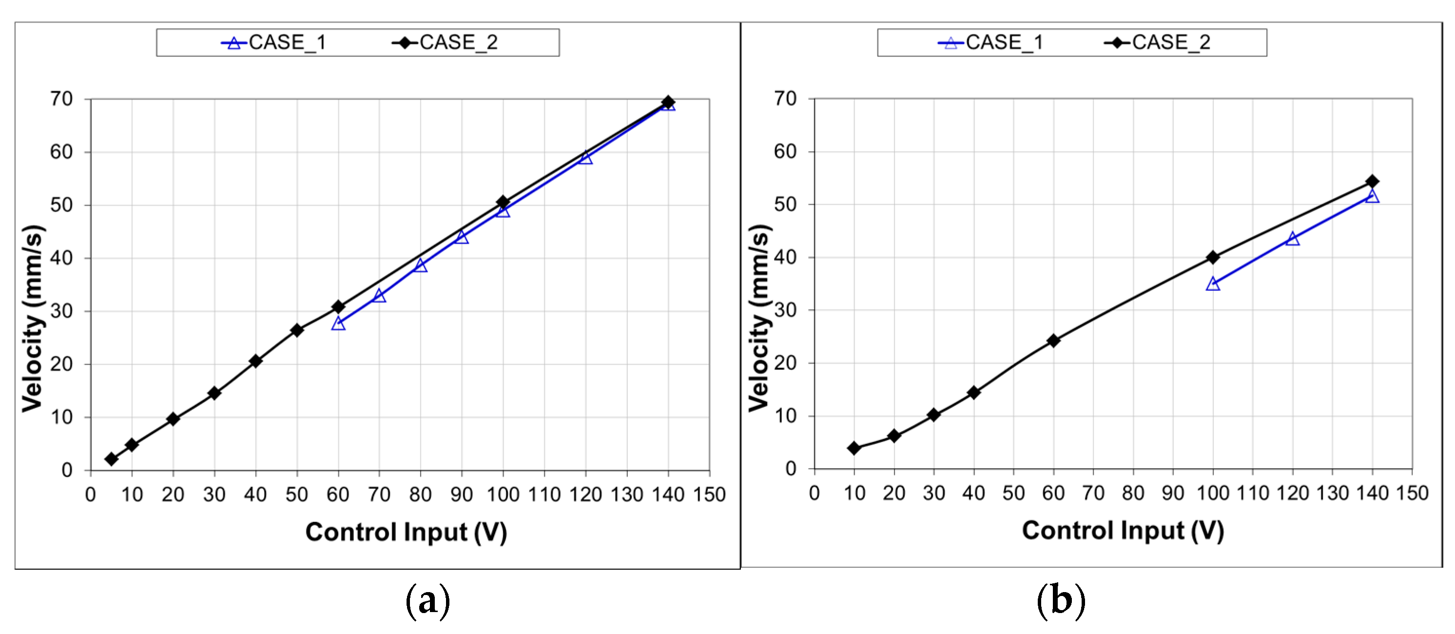
Case 1: The control input in this case was the driving signals of which one was applied between the two top and the other was applied between the two bottom electrodes. The signals on the top and the bottom electrodes were changed with equal magnitudes at the same time while keeping the phase shift between them at 90 degrees. As can be seen in Figure 15, with the speed–driving voltage (control input) curve, the threshold voltage was relatively large, and with the increase of pre-stress, the threshold voltage further increased. When the pre-stress was 35 N, the slider started to move at 60 V. When the pre-stress was increased to 70 N, the starting voltage of the slider increased to 100 V.
Case 2: The magnitude of the signal that is responsible for making normal displacement was at maximum level (160 V peak-to-peak). According to the actuator orientation, as seen in Figure 14, the signal that was applied between the two top electrodes generated displacement in the normal direction. The other signal that was applied between the two bottom electrodes generated tangential displacement, which was the control input in “Case 2” driving. Speed–control input curves were also obtained for the two different pre-stress conditions at 35 N and 70 N. As can be seen in Figure 15, case 2 driving had smaller dead-zones, or smaller threshold voltages. When the pre-stress force was 35 N, the control input threshold voltage decreased to 5 V from 60 V. Although, the pre-stress was increased to 70 N, the control input threshold voltage decreased to 10 V from 100 V.
2.3. Load Characteristics
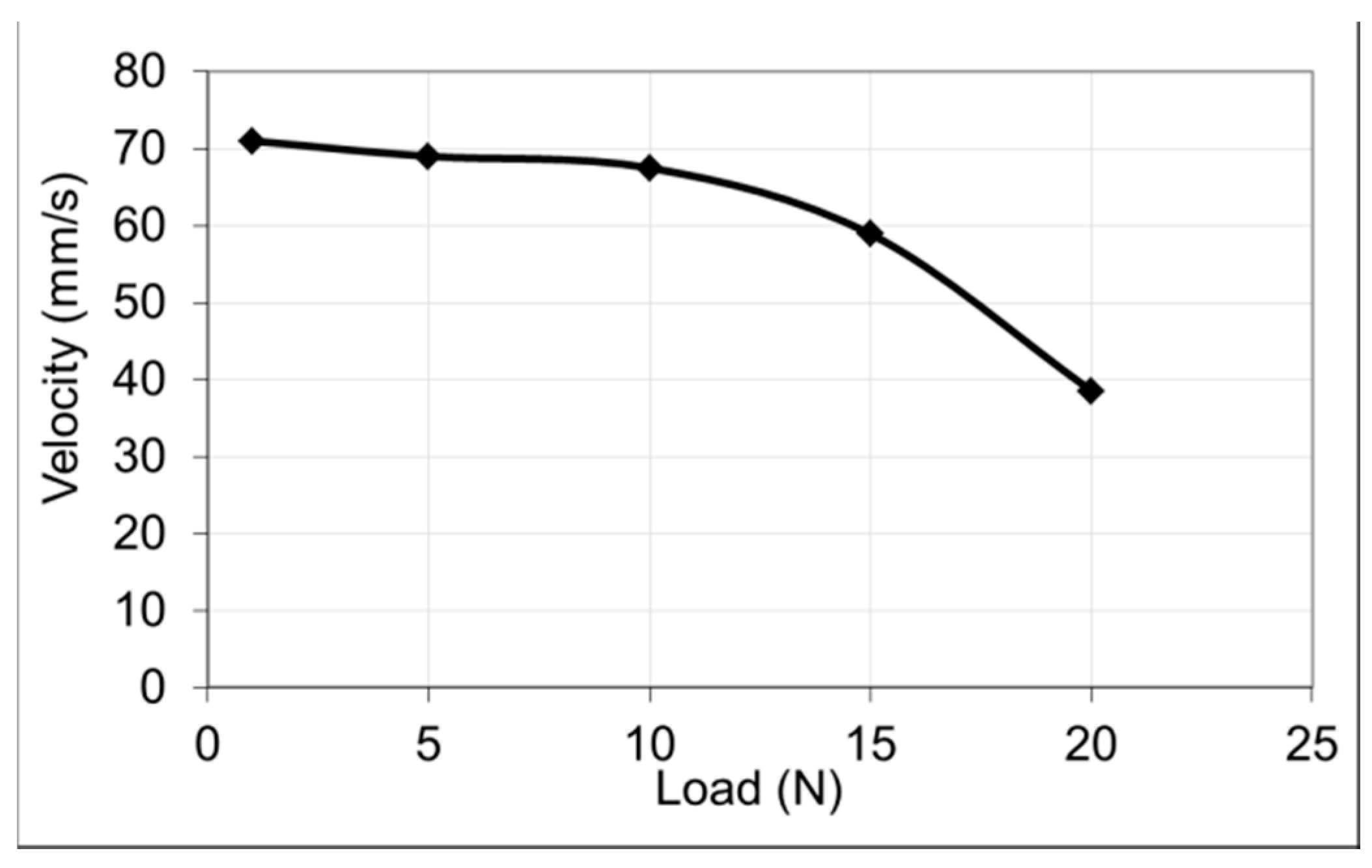
In order to obtain load characteristics, the test motor was driven under different load conditions (1, 5, 10, 20 N) and a series of position data was collected by the embedded encoder. When the magnitude of the signal responsible for generating displacement in the normal direction was 160 V, and the magnitude of the signal responsible for generating displacement in the tangential direction was 140 V (peak to peak), the motor speeds were calculated from the measured position data. A typical load characteristic of the test motor is shown in Figure 16. Even though the main purpose in this study was to reduce speed–control input (driving voltage) nonlinearities, the test motor can produce a maximum force of 20 N and a maximum speed of 70 mm/s.
3. Conclusions
Although there are piezoelectric motors with various structures, there are not many operating principles which cause them to be categorized as piezo-walk-drive, inertia-drive and resonance-drive types. In the case of the piezo-walk-drive, normal and tangential displacements (thus forces) at the interface are performing “clamp-release-move” or “while clamping push” steps. In the case of the inertia-drive, only a tangential displacement or a direction-dependent tangential force change at the interface is enough to obtain movement. For the resonance-drive, microscopic displacement at the interface has tangential and normal components, where magnitudes and phase difference between these displacements determine the direction of microscopic movements.
The resonance-drive type piezoelectric motor introduced in this study covers both single and multi-mode operation types. Oblique motion at the interface is just a special case when the phase difference is either 0 or 180 degrees.
Microscopic movement at the stator–slider interface of the new resonance piezoelectric motor is fully controllable, with the phase shifts and magnitude of the surface driving signals on the octagonal plate. By driving the top and bottom electrodes with different frequencies (w1 and w2) at the interface, even complex movements, other than oblique or elliptical, are also possible.
Author Contributions
Two authors write this paper together.
Conflicts of Interest
The authors declare no conflict of interest.
References
- Uchino, K.; Giniewica, J.R. Micromechatronics; Marcel Dekker Inc.: New York, NY, USA, 2003. [Google Scholar]
- Ervin, E. (Ed.) Vibro-Motors for Precision Micro-Robots; Hemisphere Publishing Co.: Carlsbad, CA, USA, 1988. [Google Scholar]
- Ueha, S.; Tomikawa, Y. Ultrasonic Motors—Theory and Applications; Oxford University Press: Oxford, UK, 1993. [Google Scholar]
- Sashida, T.; Kenjo, T. An Introduction to Ultrasonic Motors; Oxford University Press: Oxford, UK, 1993. [Google Scholar]
- Zhao, C. Ultrasonic Motors: Technologies and Applications; Science Press: Beijing, China; Springer: Berlin, Germany, 2011. [Google Scholar]
- Spanner, K.; Koc, B. Piezoelectric Motors, an Overview. Actuators 2016, 5, 6. [Google Scholar] [CrossRef]
- Hunstig, M. Piezoelectric Inertia Motors—A Critical Review of History, Concepts, Design, Applications, and Perspectives. Actuators 2017, 6, 7. [Google Scholar] [CrossRef]
- Peng, Y.; Peng, Y.; Gu, X.; Wang, J.; Yu, H. A Review of Long Range Piezoelectric Motors using Frequency Leveraged Method. Sens. Actuators A Phys. 2015, 235, 240–255. [Google Scholar] [CrossRef]
- Zhang, Z.M.; An, Q.; Li, J.W.; Zhang, W.J. Piezoelectric Friction–Inertia Actuator—A Critical Review and Future Perspective. Int. J. Adv. Manuf. Technol. 2012, 62, 669–685. [Google Scholar] [CrossRef]
- Morita, T. Miniature Piezoelectric Motors. Sens. Actuators A Phys. 2003, 103, 291–300. [Google Scholar] [CrossRef]
- Watson, B.; Friend, J.; Yeo, L. Piezoelectric Ultrasonic Micro/Milli Scale Actuators. Sens. Actuators A Phys. 2009, 152, 219–233. [Google Scholar] [CrossRef]
- We Evolve Our Ultrasonic Motor. Available online: http://www.shinsei-motor.com/English/index.html (accessed on 10 August 2017).
- Nanomotion. Available online: http://www.nanomotion.com/ (accessed on 10 August 2017).
- PI Products. Available online: https://www.physikinstrumente.com/en/products/ (accessed on 10 August 2017).
- Piezomotor. Available online: http://www.piezomotor.com/ (accessed on 10 August 2017).
- Newscaletech. Available online: https://www.newscaletech.com/ (accessed on 10 August 2017).
- Brisbane, A.D. Position Control Device. U.S. Patent 3,377,489, 9 April 1965. [Google Scholar]
- Hsu, K.; Biatter, A. Transducer. U.S. Patent 3,292,019, 13 December 1966. [Google Scholar]
- Locher, G.L. Micrometric Linear Actuator. U.S. Patent 3,296,467, 3 January 1967. [Google Scholar]
- Galutva, G.V.; Ryazantsev, A.I.; Presnyakov, G.S.; Modestov, J.K. Device for Precision Displacement of a Solid Body. U.S. Patent 3,684,904, 15 April 1970. [Google Scholar]
- May, W.G. Piezoelectric Electromechanical Translation Apparatus. U.S. Patent 3,902,084, 30 May 1974. [Google Scholar]
- Shamoto, E.; Shin, H.; Moriwaki, T. Development of Precision Feed Mechanism by Applying Principle of Walking Drive (1st Report)—Principle and Basic Performance of Walking Drive. J. JSPE 1993, 59, 317–322. (In Japanese) [Google Scholar]
- Marth, H.; Gloess, R. Verstelleantrieb aus Bimorphelementen. DE Patent 4,408,618A1, 15 March 1994. [Google Scholar]
- Bexell, M.; Johansson, S. Characteristics of a Piezoelectric Miniature Motor. Sens. Actuators A Phys. 1999, 75, 118–130. [Google Scholar] [CrossRef]
- Li, J.; Zhou, X.; Zhao, H.; Shao, M.; Hou, P.; Xu, X. Design and Experimental Performances of a Piezoelectric Linear Actuator by Means of Lateral Motion. Smart Mater. Struct. 2015, 24, 065007. [Google Scholar] [CrossRef]
- Cheng, T.; He, M.; Li, H.; Lu, X.; Zhao, H.; Gao, H. A Novel Trapezoid-Type Stick-Slip Piezoelectric Linear Actuator Using Right Circular Flexure Hinge Mechanism. IEEE Trans. Ind. Electron. 2017, 64, 5545–5552. [Google Scholar] [CrossRef]
- Stibitz, R. Incremental Feed Mechanisms. U.S. Patent 3,138,749, 23 June 1964. [Google Scholar]
- Thaxter, J.B. Piezoelectric Wafer Mover. U.S. Patent 4,195,243, 25 May 1980. [Google Scholar]
- Pohl, D.W. Dynamic Piezoelectric Transducer Devices. Rev. Sci. Instrum. 1987, 58, 54. [Google Scholar] [CrossRef]
- Higuchi, T.; Watanabe, M. Apparatus for Effecting Fine Movement by Impact Force Produced by Piezoelectric or Electrostrictive Element. U.S. Patent 4,894,579, 29 May 1987. [Google Scholar]
- Niedermann, P.; Emch, R.; Descouts, P. Simple Piezoelectric Translation Device. Rev. Sci. Instrum. 1988, 59, 368–369. [Google Scholar] [CrossRef]
- Yamagata, Y.; Higuchi, T.; Saeki, H.; Ishimaru, H. Ultrahigh Vacuum Precise Positioning Device Utilizing Rapid Deformations of Piezoelectric Elements. J. Vac. Sci. Technol. A 1990, 8, 4098–4100. [Google Scholar] [CrossRef]
- Renner, C.H.; Niedermann, P.H.; Kent, A.D.; Fischer, O. A Vertical Piezoelectric Inertial Slider. Rev. Sci. Instrum. 1990, 61, 965–967. [Google Scholar] [CrossRef]
- Howald, L.; Rudin, R.; Guntherodt, H.-J. Piezoelectric Inertial Stepping Motor with Spherical Rotor. Rev. Sci. Instrum. 1992, 63, 3909–3912. [Google Scholar] [CrossRef]
- Blackford, B.L. A Simple Self-Propelled Two-Dimensional Micropositioner. Rev. Sci. Instrum. 1993, 64, 1360–1361. [Google Scholar] [CrossRef]
- Tapson, J.; Greene, J.R. A Simple Dynamic Piezoelectric x-y Translation Stage Suitable for Scanning Probe Microscopes. Rev. Sci. Instrum. 1993, 64, 2387–2388. [Google Scholar] [CrossRef]
- Libioulle, L.; Ronda, A.; Derycke, I.; Vigneron, J.P.; Gilles, J.M. Vertical Two-Dimensional Piezoelectric Inertial Slider for Scanning Tunneling Microscope. Rev. Sci. Instrum. 1993, 64, 1489–1494. [Google Scholar] [CrossRef]
- Miyano, M.; Kawasaki, T.; Kuwana, M.; Miyazawa, M.; Ueyama, M.; Tasaka, Y. Lens Moving Apparatus. U.S. Patent 5,587,846, 14 July 1995. [Google Scholar]
- Kleindiek, S. Electromechanical Drive Element Comprising a Piezoelectric Element. U.S. Patent 6,741,011, 3 March 2000. [Google Scholar]
- Karrai, K.; Heines, M. Inertial Rotation Device. U.S. Patent 6,940,210B2, 22 November 2001. [Google Scholar]
- Meyer, C.; Sqalli, O.; Lorenz, H.; Karrai, K. Slip-Stick Step-Scanner for Scanning Probe Microscopy. Rev. Sci. Instrum. 2005, 76, 063706. [Google Scholar] [CrossRef]
- Müller, K.D.; Marth, H.; Pertsch, R.; Gloss, R.; Zhao, X. Piezo-Based, Long-Travel Actuators for Special Environmental Conditions. In Proceedings of the 10th International Conference on New Actuators, Bremen, Germany, 14–16 June 2006; pp. 149–153. [Google Scholar]
- Thomas, P.; Desailly, R. Optical Adjustment Mounts with Piezoelectric Inertia Driver. U.S. Patent WO 2008087469A2, 18 January 2007. [Google Scholar]
- Huebner, R. Piezoelectric rotary Drive for A Shaft. U.S. Patent 9,106,158, 1 August 2012. [Google Scholar]
- Kortschack, A.; Rass, C. Method for Controlling A Multi-Actuator Drive. German Patent WO2013128032A1, 4 March 2013. [Google Scholar]
- Hunstig, M.; Hemsel, T.; Sextro, W. Stick-Slip and Slip-Slip Operation of Piezoelectric Inertia Drives. Part I: Ideal Excitation. Sens. Actuators A Phys. 2013, 200, 90–100. [Google Scholar] [CrossRef]
- Hunstig, M.; Hemsel, T.; Sextro, W. Stick-Slip and Slip-Slip Operation of Piezoelectric Inertia Drives—Part II: Frequency-Limited Excitation. Sens. Actuators A Phys. 2013, 200, 79–89. [Google Scholar] [CrossRef]
- Meissner, A. Converting Electrical Oscillations into Mechanical Movement. U.S. Patent 1,804,838, 26 May 1927. [Google Scholar]
- Williams, A.L.W.; Brown, W.J. Piezoelectric Motor. U.S. Patent 2,439,499, 13 April 1948. [Google Scholar]
- Lavrinenko, V.; Nekrasov, M. Electrical Motor. USSR Patent 217,509, 10 May 1965. [Google Scholar]
- Tehon, S.W. Electromechanical Transducer Motors. U.S. Patent 3,211,931, 12 October 1965. [Google Scholar]
- Wischnewsky, V.; Kavertsev, V.L.; Kartashev, I.A.; Lavrinenko, V.; Nekrasov, M.; Prez, A.A. Piezoelectric Motor Structures. U.S. Patent 4,019,073, 10 April 1975. [Google Scholar]
- Barth, H.V. Ultrasonic Drive Motor. IBM Tech. Discl. Bull. 1973, 16, 2263. [Google Scholar]
- Wischnewskiy, V.; Gultajeva, L.; Kartashev, I.; Lavrinenko, V. Piezoelectric Motor. USSR Patent 851,560, 16 February 1976. [Google Scholar]
- Bansiavichus, R. Piezoelectric Motor. USSR Patent 693,493, 18 July 1977. [Google Scholar]
- Bansevičius, B.; Blechertas, V. Ultrasonic Motors for Mass-Consumer Products. ULTRAGARSAS 2006, 4, 1392–2114. [Google Scholar]
- Ko, H.P.; Lee, K.J.; Yoo, K.H.; Kang, C.Y.; Kim, S.; Yoon, S.J. Analysis of Tiny Piezoelectric Ultrasonic Linear Motor. Jpn. J. Appl. Phys. 2006, 45, 4782–4786. [Google Scholar] [CrossRef]
- Morita, T.; Nishimura, T.; Yoshida, R.; Hosaka, H. Resonant-Type Smooth Impact Drive Mechanism Actuator Operating at Lower Input Voltages. Jpn. J. Appl. Phys. 2013, 52, 07HE05. [Google Scholar] [CrossRef]
- Koc, B. Piezoelectric Motor, Operates by Exciting Multiple Harmonics of a Square Plate. In Proceedings of the 12th International Conference on New Actuators, Bremen, Germany, 14–16 June 2010. [Google Scholar]
- Tuncdemir, S.; Ural, S.O.; Koc, B.; Uchino, K. Design of Translation Rotary Ultrasonic Motor with Slanted Piezoelectric Ceramics. Jpn. J. Appl. Phys. 2011, 50, 027301. [Google Scholar] [CrossRef]
- Galante, T.; Frank, J.; Bernard, J.; Chen, W.; Lesieutre, G.A.; Koopmann, G.H. Design, Modeling, and Performance of a High Force Piezoelectric Inchworm Motor. J. Intell. Mater. Syst. Struct. 1999, 10, 962–972. [Google Scholar] [CrossRef]
- Egashira, Y.; Kosaka, K.; Iwabuchi, T.; Kosaka, T.; Baba, T.; Endo, T.; Hashiguchi, H.; Harada, T.; Nagamoto, K.; Watanabe, M.; et al. Sub-Nanometer Resolution Ultrasonic Motor for 300 mm Wafer Lithography Precision Stage. Jpn. J. Appl. Phys. 2002, 41, 5858–5863. [Google Scholar] [CrossRef]
- Koc, B. An Ultrasonic Motor Using Side-Push of Centre-Attached Eyelets on an Octagonal Piezoelectric Plate. In Proceedings of the 16th International Conference on New Actuators, Bremen, Germany, 25–27 June 2018. [Google Scholar]
Figure 1.
Motion sequences of a piezo-walk-drive motor proposed by Brisbane in 1965 [17].
Figure 1.
Motion sequences of a piezo-walk-drive motor proposed by Brisbane in 1965 [17].

Figure 2.
Motion sequences of a piezo-walk-drive motor proposed by Shamoto in 1993 [22].
Figure 2.
Motion sequences of a piezo-walk-drive motor proposed by Shamoto in 1993 [22].

Figure 3.
Inertia-drive piezoelectric motor proposed by Pohl in 1986 [29].
Figure 3.
Inertia-drive piezoelectric motor proposed by Pohl in 1986 [29].
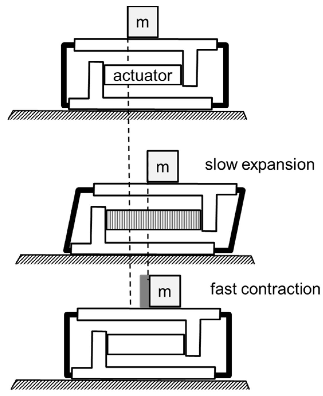
Figure 4.
Inertia-drive piezoelectric motor proposed by Higuchi in 1986 [30].
Figure 4.
Inertia-drive piezoelectric motor proposed by Higuchi in 1986 [30].
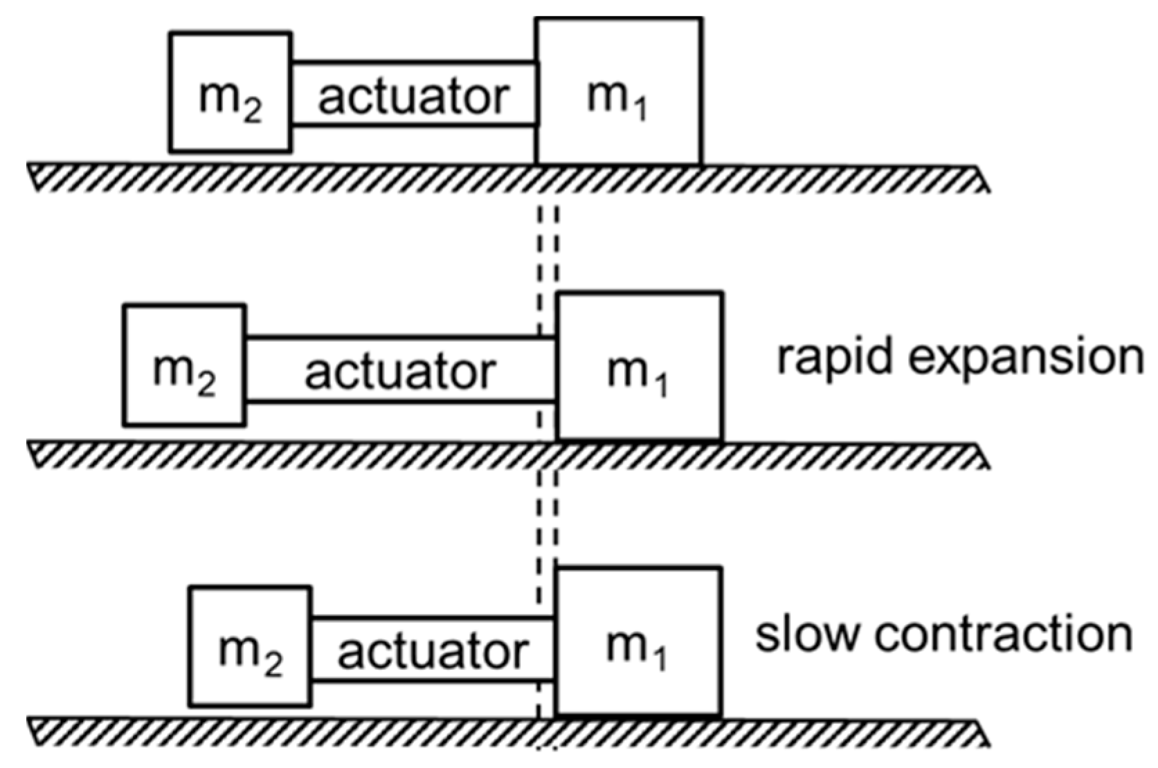
Figure 5.
In a resonance-drive type piezoelectric motor, there are elliptical or oblique motions at the stator-rotor (/slider) contact points.
Figure 5.
In a resonance-drive type piezoelectric motor, there are elliptical or oblique motions at the stator-rotor (/slider) contact points.

Figure 6.
(a) Metallization electrodes are oriented orthogonally on the main surfaces of the octagonal piezoelectric plate. (b) The coupling elements are two eyelets that are attached in the middle of the two main surfaces on the octagonal piezoelectric plate. The side surfaces of the eyelets (marked with red arrows) are in contact with the slider.

Figure 7.
Electric fields in the four regions of the octagonal piezoelectric plate when the magnitudes A, B and thickness d are normalized to 1. Frequencies ( and ) for both signals are assumed to be equal and T is the period (phase shift () is 90 degrees).
Figure 7.
Electric fields in the four regions of the octagonal piezoelectric plate when the magnitudes A, B and thickness d are normalized to 1. Frequencies ( and ) for both signals are assumed to be equal and T is the period (phase shift () is 90 degrees).

Figure 8.
In-plane first and second mode shapes when only the bottom surface electrodes are electrically excited. Deformations are in the x-axis direction. (a) First in-plane mode at 68 kHz, (b) Second in-plane mode at 154.5 kHz.
Figure 8.
In-plane first and second mode shapes when only the bottom surface electrodes are electrically excited. Deformations are in the x-axis direction. (a) First in-plane mode at 68 kHz, (b) Second in-plane mode at 154.5 kHz.

Figure 9.
In-plane first and second mode shapes when only the top electrodes are electrically excited. Deformations are in the y-axis direction. (a) First in-plane mode at 68 kHz, (b) Second in-plane mode at 154.5 kHz.
Figure 9.
In-plane first and second mode shapes when only the top electrodes are electrically excited. Deformations are in the y-axis direction. (a) First in-plane mode at 68 kHz, (b) Second in-plane mode at 154.5 kHz.

Figure 10.
Calculated motion trajectories at first (68.7 kHz) and second (154.5 kHz) resonance modes.
Figure 10.
Calculated motion trajectories at first (68.7 kHz) and second (154.5 kHz) resonance modes.
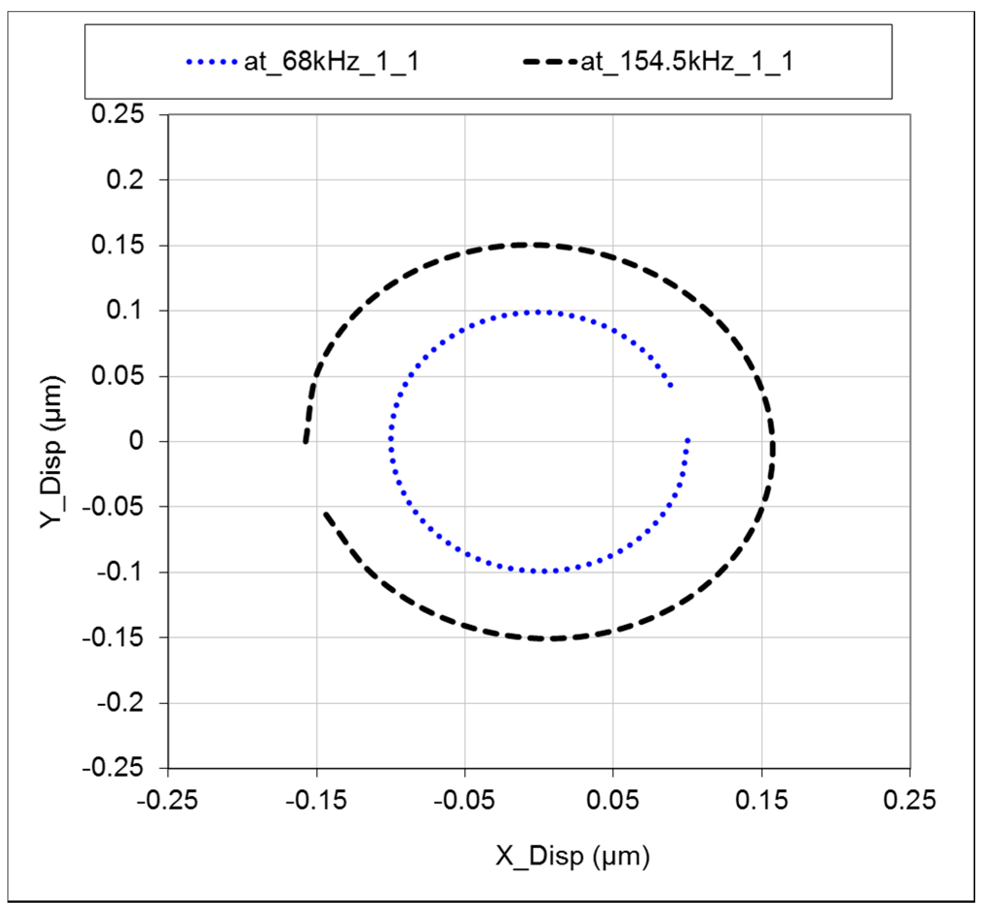
Figure 11.
Calculated motion trajectories, when the magnitude of the signals applied on the top or on the bottom electrodes is changed.
Figure 11.
Calculated motion trajectories, when the magnitude of the signals applied on the top or on the bottom electrodes is changed.
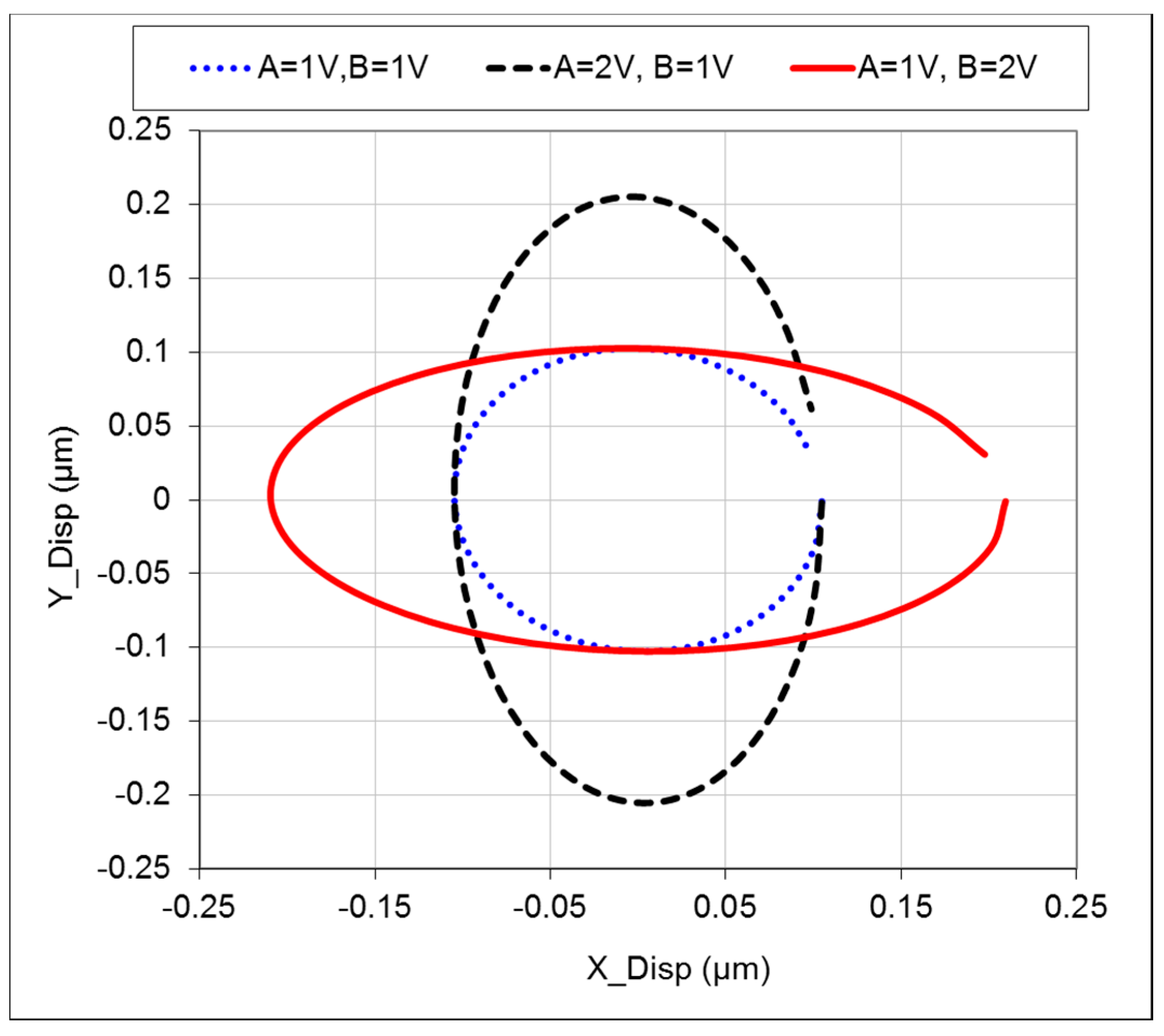
Figure 12.
Response of the trajectory to the phase shift between the signals on the top and bottom electrodes.
Figure 12.
Response of the trajectory to the phase shift between the signals on the top and bottom electrodes.

Figure 13.
Perspective and end views of the vibrator–slider interface. The side surfaces of both eyelets were contacted tangentially to the alumina rods on the U-shaped slider. The distance between any of the two parallel side surfaces of the plate was 25 mm and the thickness was 3.0 mm.
Figure 13.
Perspective and end views of the vibrator–slider interface. The side surfaces of both eyelets were contacted tangentially to the alumina rods on the U-shaped slider. The distance between any of the two parallel side surfaces of the plate was 25 mm and the thickness was 3.0 mm.

Figure 14.
Perspective views (3D CAD drawing and photo) of the test linear motor. The piezoelectric vibrating element was placed between two identical holders.
Figure 14.
Perspective views (3D CAD drawing and photo) of the test linear motor. The piezoelectric vibrating element was placed between two identical holders.

Figure 15.
Speed–driving voltage (control input) characteristics for two cases of driving. (a) Pre-stress in the normal direction: 35 N, (b) Pre-stress in the normal direction: 70 N.
Figure 15.
Speed–driving voltage (control input) characteristics for two cases of driving. (a) Pre-stress in the normal direction: 35 N, (b) Pre-stress in the normal direction: 70 N.

Figure 16.
Load characteristics of the test linear motor. Sinusoidal wave signals generating normal and tangential displacements have magnitudes of 160 and 140 V (peak-to-peak), respectively.
Figure 16.
Load characteristics of the test linear motor. Sinusoidal wave signals generating normal and tangential displacements have magnitudes of 160 and 140 V (peak-to-peak), respectively.
© 2018 by the authors. Licensee MDPI, Basel, Switzerland. This article is an open access article distributed under the terms and conditions of the Creative Commons Attribution (CC BY) license (http://creativecommons.org/licenses/by/4.0/).
Share and Cite
MDPI and ACS Style
Spanner, K.; Koc, B. Piezoelectric Motor Using In-Plane Orthogonal Resonance Modes of an Octagonal Plate. Actuators 2018, 7, 2. https://doi.org/10.3390/act7010002
AMA Style
Spanner K, Koc B. Piezoelectric Motor Using In-Plane Orthogonal Resonance Modes of an Octagonal Plate. Actuators. 2018; 7(1):2. https://doi.org/10.3390/act7010002
Chicago/Turabian StyleSpanner, Karl, and Burhanettin Koc. 2018. "Piezoelectric Motor Using In-Plane Orthogonal Resonance Modes of an Octagonal Plate" Actuators 7, no. 1: 2. https://doi.org/10.3390/act7010002
Note that from the first issue of 2016, this journal uses article numbers instead of page numbers. See further details here.