The Central Italy Electromagnetic Network and the 2009 L'Aquila Earthquake: Observed Electric Activity

Abstract
: A network of low frequency electromagnetic detectors has been operating in Central Italy for more than three years, consisting of identical instruments that continuously record the electrical components of the electromagnetic field, ranging from a few Hz to tens of kHz. These signals are analyzed in real time and their power spectrum contents and time/frequency data are available online. To date, specific interest has been devoted to searching for any possible electromagnetic features which correlate with seismic activity in the same region. In this study, spectral analysis has evidenced very distinct power spectrum signatures that increased in intensity when strong seismic activity occurred near the stations of the 2009 L'Aquila earthquake. These signatures have revealed horizontally oriented electric fields, between 20 Hz to 400 Hz, lasting from several minutes to up to two hours. Their power intensities have been found to be about 1 μV/m. Moreover, a large number of man-made signals and meteorologic electric perturbations were recorded. Anthropogenic signatures have come from power line disturbances at 50 Hz and higher harmonics up to several kHz, while radio transmissions have influenced the higher kHz spectrum. Reception from low frequency transmitters is also provided in relation to seismic activity. Meteorologic signatures cover the lower frequency band through phenomena such as spherics, Schumann resonances and rain electrical perturbations. All of these phenomena are useful teaching tools for introducing students to this invisible electromagnetic world.1. Introduction
Instrumental studies of earthquake electric phenomena began in the 1800s in Italy [1,2]. These studies were inspired by several observations reported in 18th century collections of earthquake phenomena [3,4], thanks to the pioneers of electricity in Italy at that time, as well as the inventions of instruments to record electric and magnetic fields [5]. The developments of earthquake predicting tools began at that time [6] and continued through the next century [7,8]. At that point, however, many inventors ceased to proceed because their studies were founded on the recently rooted and therefore not yet fully applied Electromagnetic (EM) theory, which contrasted with the nascent science of seismology founded on the existing inertial theory [9]. Yet, during the same years the first radio was being built, opening up an intense study on EM sources, propagation and absorptions [10]. These contributions have provided us with a set of well suited methods to address the EM study of every system, allowing for the possibility to revisit old efforts with the benefit of current EM theory.
Magnetic observations made in connection with strong earthquakes, from Immanuel Kant's writings [11] to the Edo earthquake [12], have all sustained further studies. In fact, magnetic phenomena associated to earthquakes and volcanic eruptions have been widely studied in Japan [13] and the U.S. utilizing highly sensitive instruments [14]. Some noteworthy results in the Ultra Low Frequency (ULF) band regarding very strong seismic events include the Alaska earthquake in 1964 [15] and other earthquakes which occurred near magnetic network observatories [16]. However, different interpretations for the observed ULF anomalies though a controversy erupted over their connection to the seismic events [17,18]. Furthermore, recent studies have revealed long period magnetospheric oscillations at discrete frequencies due to solar wind velocity variations, which can occur at medium latitudes [19]. Recently, efforts to follow up observations of ULF activity have been reported in Italy [20] and by QuakeFinder [21]. The QuakeFinder Network, which consists of over 50 sites in California and Peru, 15 of which are high-resolution systems, have documented increases in ULF pulse activity preceding nearby seismic events, followed by decreases in activity [21,22].
Continuous long-term EM monitoring is necessary for obtaining reliable results regarding correlations with seismic activity [23]. Here, a simple and economical recording system is proposed which is currently operative at the eight stations of the Central Italy Electromagnetic Network (CIEN). Historical observations of electric phenomena and earthquake lights (EQL) stemming from the 18th century [24–28], initially stimulated electric investigations with earthquakes. Furthermore, given that recent magnetic recordings have not provided definitive confirmation of an earthquake link, the CIEN has chosen to record the EM field via its electric component. The chosen frequency bands were in the Extremely Low Frequency (ELF) and the Very Low Frequency (VLF) ranges, for which some recent results have shown several anomalies with earthquakes [29,30].
The next section is devoted to the signals and their descriptions in connection to different phenomena. A particular and intense type of signal was recorded on the occasion of the 2009 L'Aquila earthquake; the strongest quake in Italy since CIEN began operating. This signal is analyzed to illustrate the CIEN capacity. CIEN will be described in the third section together with its instruments, so that a quantitative evaluation of previously described signals can be given. Because a single sensor is capable of detecting electric fields at several frequency bands, different types of electromagnetic perturbations observed with earthquakes [23] must be considered in this paper. The fourth section is devoted to summarizing, even if not statistically significant yet, the characteristics of the recorded signals and natural or anthropogenic phenomena.
2. CIEN Recordings and Their Discussion
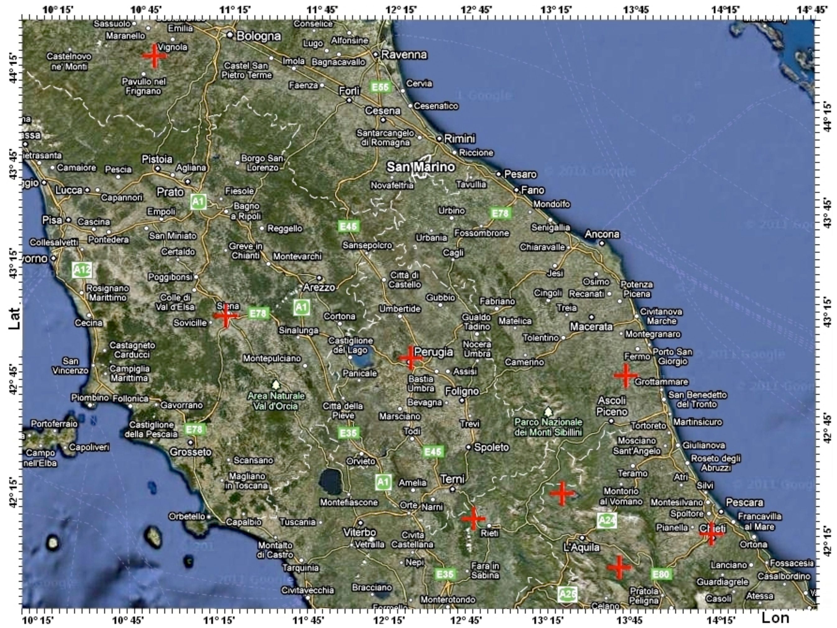
The first CIEN station began operating in San Procolo, near the city of Fermo, in the Marche Region in 2006, hereinafter, referred to as the Fermo Station. The Fermo Station was initially set up with an ELF-VLF (10 Hz–5 kHz) amplifier and a long-wave radio receiver tuned at 150 kHz. The electrode and the antenna were oriented along a North-South (N-S) direction. After four years of experimentation with several types of low frequency wide band amplifiers, the Fermo station was uniformed in 2010 to the other EM stations by substituting the radio receiver and the amplifier with a couple of ELF (4 Hz–1 kHz) inverting amplifiers where electrodes were set perpendicular to each other and oriented along N-S and East-West (E-W) directions. A second station began operations in Perugia, in the Umbria Region in 2008 with the same two amplifiers. From summer 2010 onward, two other stations began operating in Zocca, near Modena, in the Emilia Romagna Region in August 2010, and in Capitignano, near L'Aquila, in the Abruzzo Region in September 2010. In January 2011, the Chieti Station was activated at the University of Gabriele D'Annunzio, in the Abruzzo Region. In February 2011 the Siena Station began recording in the Tuscany Region. In March 2011, the Fagnano Station, near L'Aquila, in the Abruzzo Region, was activated. From October 2011, the Rieti Station has been activated in the Lazio Region. From April 2011, all of the eight stations shown in Figure 1 were updated to also record VLF (1–25 kHz) signals, while from June 2011 onward, a frequency band extension test started at the Chieti Station which is also operative in the ULF (0.04–4 Hz) and Low Frequency (LF) (25–100 kHz) bands.
2.1. CIEN Data
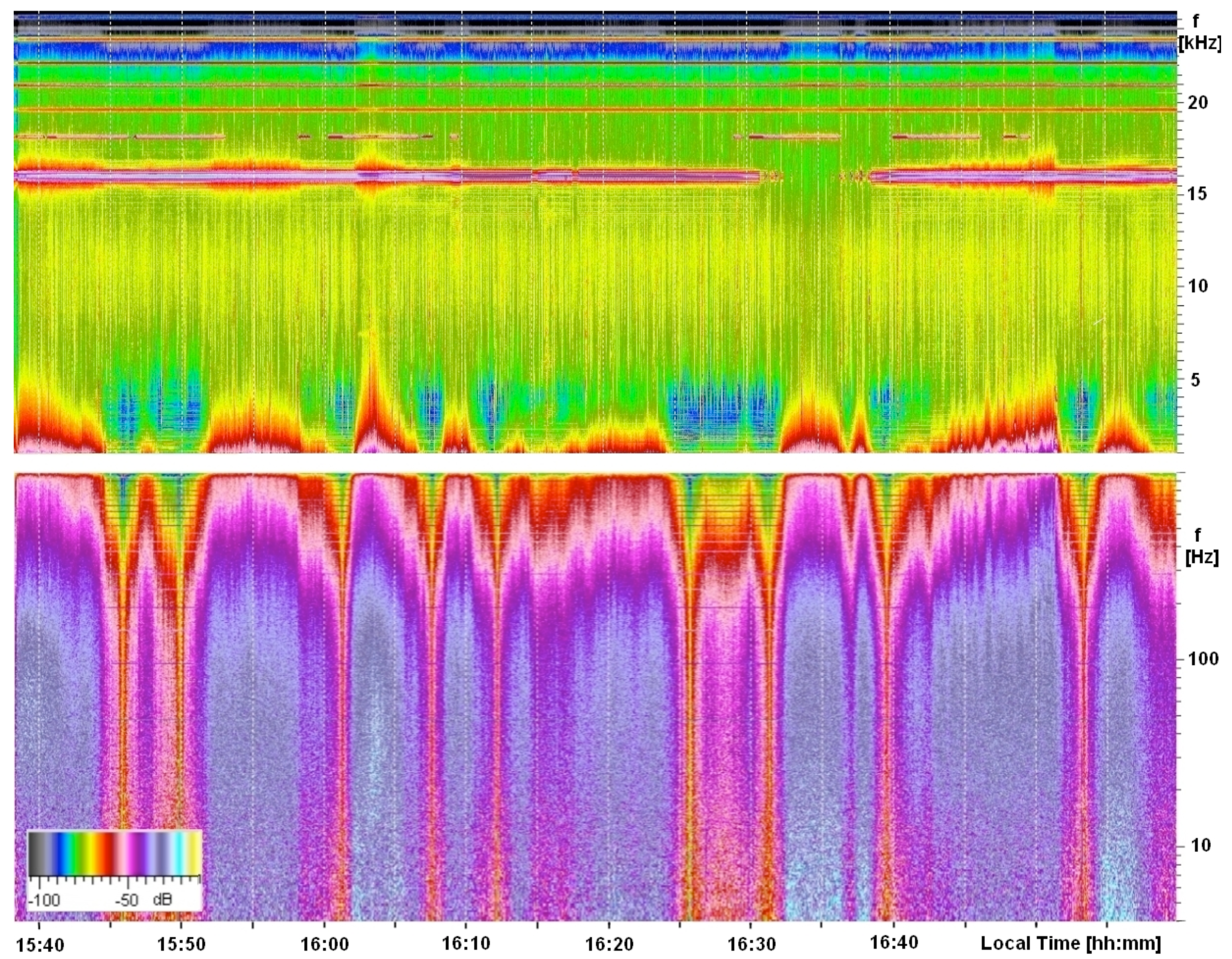
Stored data are available in two formats: wave files for recovering the complete time evolution of the signals, and jpeg files for saving the dynamical spectrum of the signals. Each specific band has its own jpeg file. Figure 2 shows the time and dynamical spectrum of the signals from one antenna at the Perugia Station. The white line in the blue band at the top of Figure 2, is the time amplitude evolution of the entire signal over a period of slightly more than one hour of recording and the vertical dotted lines indicate a five-minute intervals. The center of the plot shows the dynamical spectrum of the same signal in VLF band. Here, the vertical axis corresponds to the signal frequency in a linear scale in the range 1 kHz–25 kHz. The bottom part of the plot is the dynamical spectrum of the same signal in ELF band and, in this case, the vertical axis corresponds to the signal frequency in a logarithmic scale in the range 4 Hz–1 kHz. Logarithmic and linear scales of the spectrograms were chosen to better evidence the anomalous signals. In both of the spectrograms, power intensity is represented by different colors and measured in dB.
The strong spikes in amplitude which clearly appear in the time evolution of the signals are the strongest structures. These are evident on the ELF plot as vertical lines covering the entire frequency band, and characterized by high intensity. These are EM waves produced by lightning bolts not too far from the station [32]. Figure 2 describes a high pressure meteorological situation in the Mediterranean Sea, where sporadic perturbations occur more than 200 km away. The same spikes are limited on the VLF band, suggesting that the frequency spectrum is progressively cut by a band-pass filter over increasing distance. The green bands in both the ELF and VLF represent the numerous lightning strikes that occurred at distances of thousands of kilometers in the tropics [32].
Horizontal thin lines on the ELF represent the power supply network emission and correspond to 50 Hz with upper harmonics; these lines cover the natural signals up to about 4 kHz in the VLF band. Other less defined horizontal green/blue lines appear below 50 Hz and increase in width for lower frequencies near 10 Hz; these are known as Schumann Resonances [33]. The Earth surface and ionosphere are two conducting regions which reflect EM waves of sufficiently long lengths. Between the Earth and the ionosphere there is a closed volume where EM waves are weakly absorbed and create interference. Lightning activity is the EM source in this volume. Schumann resonances are the natural oscillations of the EM field inside the Earth-ionosphere cavity [33]. The finite frequency selection occurs at about 8, 14, 20, 26, 32, 37 and 43 Hz [33], the first resonance not always being visible as in this case. The slight contractions in the large green bands for both ELF and VLF are triggered by the ionospheric modulation due to sun illumination [34]. Finally, three gray spots, high in ELF spectrum, reflect the sub-ionosphere transmission channel modulation for VLF signals of distant lightning origins. This phenomenon is less evident in the green band of VLF.
Geometric squares on the bottom of the VLF plot reflect harmonic modulation of power line absorption, which combine odd or even harmonics to change the appearance of the plot by way of a duty cycle lasting up to four minutes. Many distinct thin horizontal lines are also present on VLF, reflecting the carrier waves of VLF transmitters which are in some cases non-continuous. Identifiable transmitters are indicated by white arrows and include [35]: Alpha 500 kW radio navigation system in Novosibirsk, Krasnodar and Khabarovsk, Russia at 11.905 kHz, 12.649 kHz and 14.881 kHz; 400 kW in Rosnay, France at 15.1 kHz and 21.75 kHz; 100 kW in Matotchkinchar, Russia at 18.1 kHz; 400 kW in Anthorn/Skelton, England at 19.6 kHz and 22.1 kHz; 400 kW in Saint-Assise, France at 20.9 kHz; 800 kW in Rhauderfehn, Germany at 23.4 kHz; 1,000 kW in Culter, Maine at 24.0 kHz and 192 kW in Seattle, Washington at 24.6 kHz. The 16 kHz signal is an emission from the photovoltaic power facility at the Perugia Station, which runs during daytime, and overlies the 45 kW VLF transmitter located in Kolsas, Norway, at 16.4 kHz.
2.2. ELF Anomalies Recorded During the L'Aquila Earthquake and Other Seismic Activity
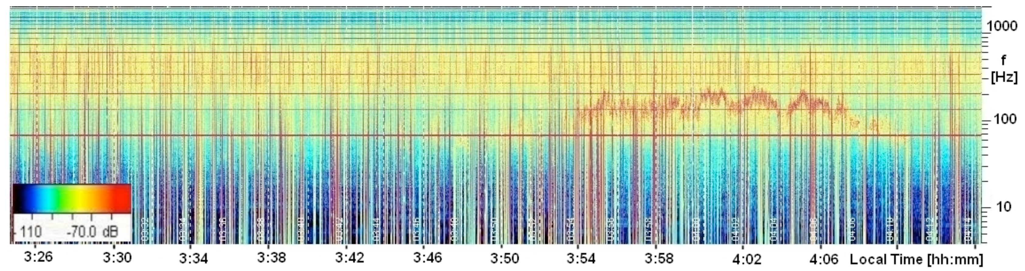
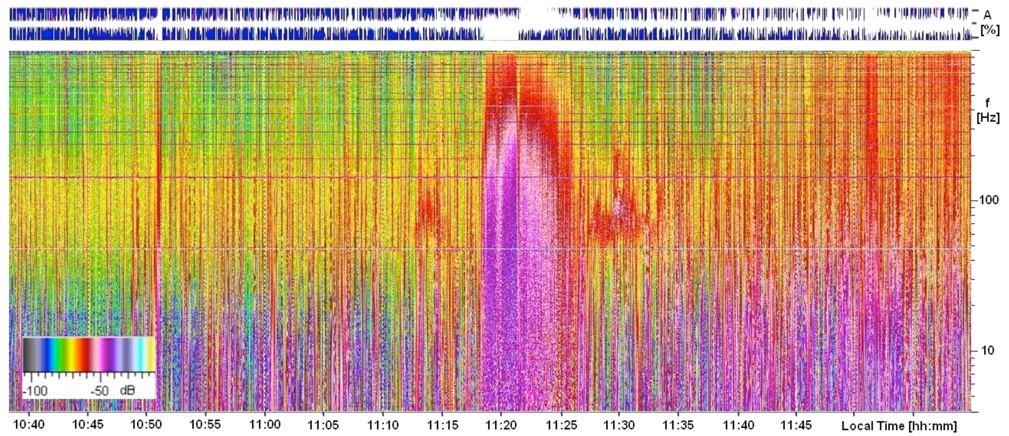
During the swarm of the L'Aquila earthquake in 2009 only two stations were running, the Fermo and Perugia Stations [36]. The Fermo Station had been active from mid-2006, and provided several examples of unknown signals with a similar frequency spectrum as observed after the main shock. Even though the Perugia Station had been active for less than one year, the same anomalies seen in Fermo were also present in Perugia, about 100 km north of L'Aquila, during the weeks before and after the main shock. The N-S antenna spectrogram from Perugia around the time of the main shock, at 3:32LT on 6 April 2009 [37], is plotted in Figure 3. Here, an intense oscillation is shown, ranging from 50 to 150 Hz, beginning about 20 min after the main shock and lasting for about 15 min.
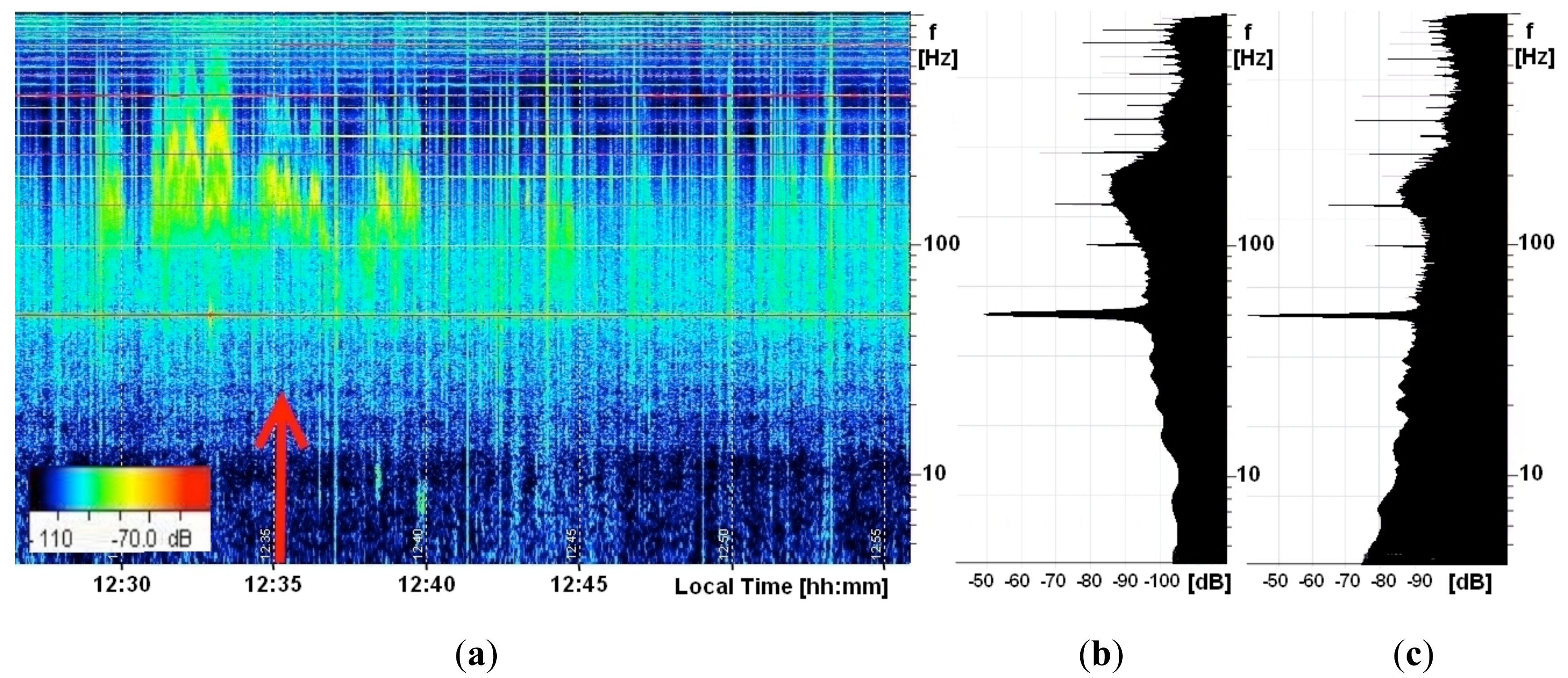
A similar signature was seen before the main L'Aquila shock also in Perugia recordings; see the spectrograms already presented for Perugia, and Fermo [36,38]. A strong signal recorded by the N-S antenna in Fermo on 2 April 2009, at about 7:50LT, is shown in Figure 4. These oscillations have similar frequencies to those in Figure 3, ranging between 20 and 200 Hz. Moreover, the duration of the signal is about 8 min, as well, weaker traces of it appearing minutes before and after the strong phase. Figures 3 and 4 share another significant similarity: their frequencies increase at the beginning, but decrease toward the end. However, no time correspondence was found between the signals of the two stations, indicating that they are of local origin. The signatures appeared nearly always on only one antenna of each station and when appearing in both antenna directions the two signatures were always different. Unlike Figure 2, the frequencies of the spectrograms in Figures 3 and 4 reach 2 kHz and their time vertical grids, represented by white dashed lines, are two minutes and one minute respectively. Furthermore, the amplitude color scales of Figures 3 and 4 are not the same as in Figure 2.
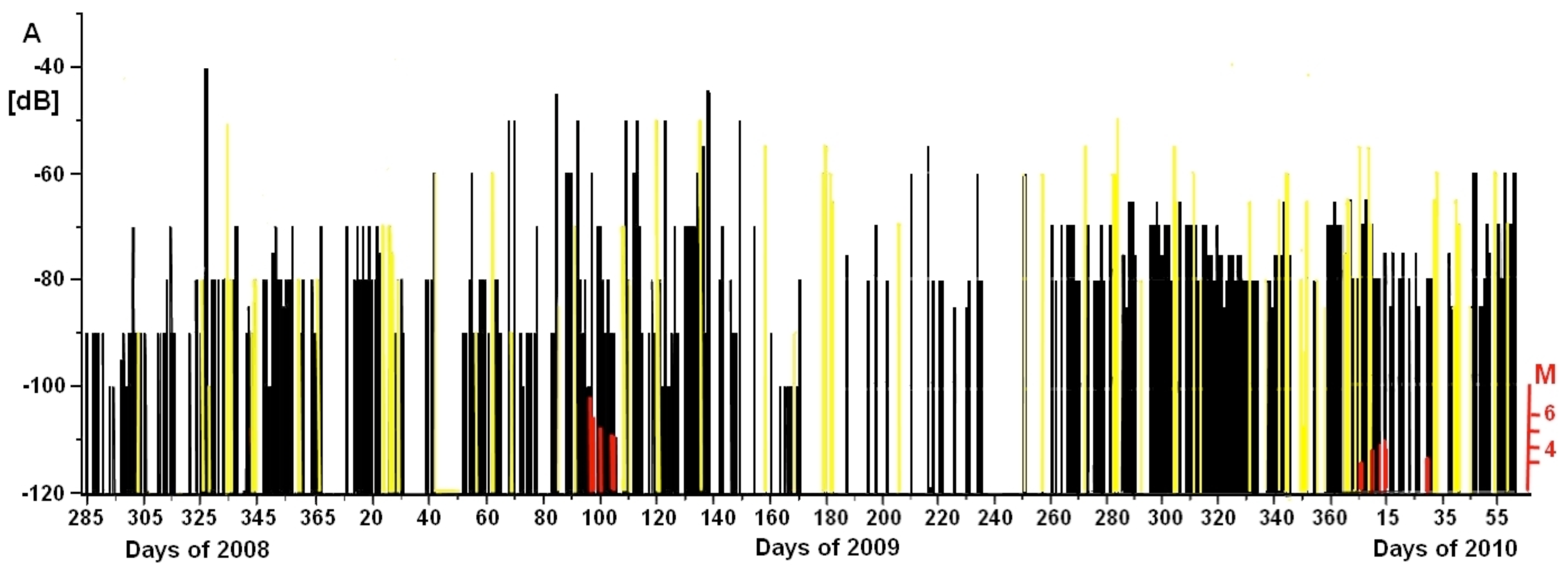
A longer term overview of the ELF data shows that similar signals also appeared in the local records several months before and after the main shock. For this, the time evolution of signal amplitudes and time lengths were studied. Calculating the daily maximum duration of the electric oscillations and plotting their distributions months before and after the April 2009, no association was evidenced with the times of main L'Aquila shocks. On the other hand, plotting the daily maximum power spectrum amplitudes of the oscillations shows a maximum near 6 April 2009. The Fermo Station amplitude distribution, between October 2008 and February 2010, is shown in Figure 5. Here, there is a trend toward increasing amplitudes over the course of six months before April 2009, the month of the L'Aquila earthquake. Red bars indicate the magnitude of the seismic events occurring in Central Italy when Dobrovolsky radius [39] is greater than the distance from the Fermo Station. The maximum amplitude power spectrum remained elevated from the end of March to mid June 2009, while during the same period all of the principal M > 5 aftershocks of the L'Aquila event occurred [37]. Afterwards, ELF maximum amplitude had a slow decline. Perugia recordings reached a maximum during the same period, even if this station had only been activated recently and was not running full-force, thereby leading to gaps in the data.
2.3. VLF Network Applications for Earthquake Study
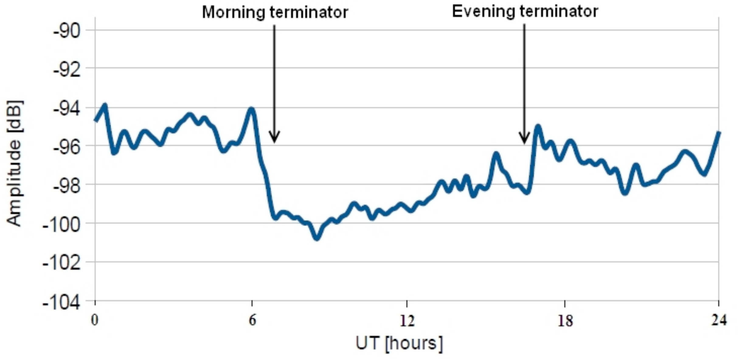
CIEN has been recently updated in the VLF band, in order to obtain EM monitoring of ionospheric effects of earthquakes [23]. Use of a VLF transmitter monitoring in connection with strong earthquakes has been studied by several authors over the last two decades, recently leading to an international cooperation which includes a network that covers the whole of Europe [29]. The project aim is to monitor the sub-ionospheric channels between VLF radio transmitters and receivers. In fact, sub-ionospheric channels, which are above the preparation zone of a future strong earthquake, have been observed in several cases preventing the transmissions many days before the main shocks. An example of daily carrier wave amplitude of Alpha transmitters is shown in Figure 6. The steps in amplitudes at about 7UT and 18UT indicate the terminator passage which is associated with ionosphere changes in the signal propagation, whereas, the steps time distance was also studied in connection with earthquakes [40].
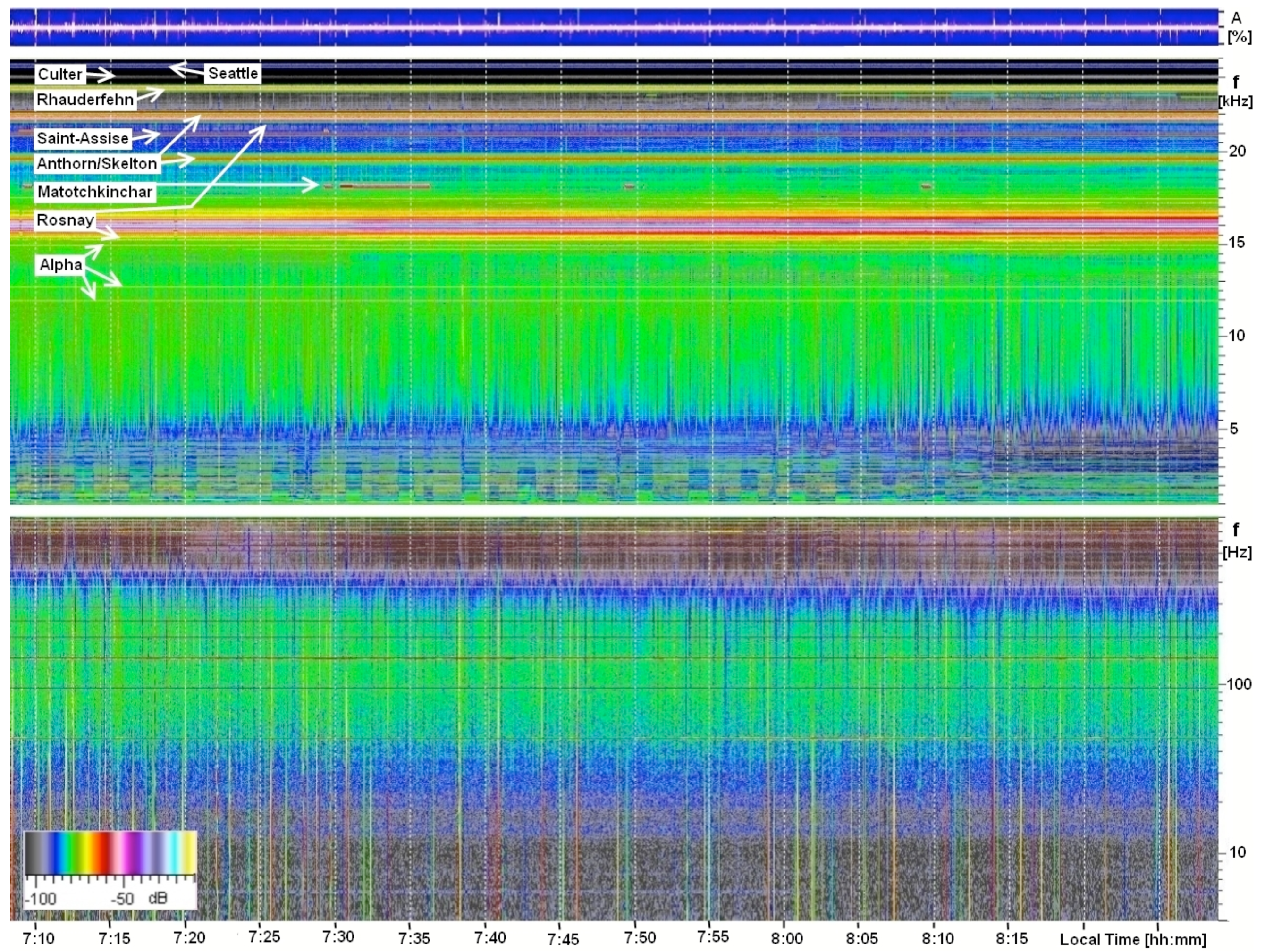
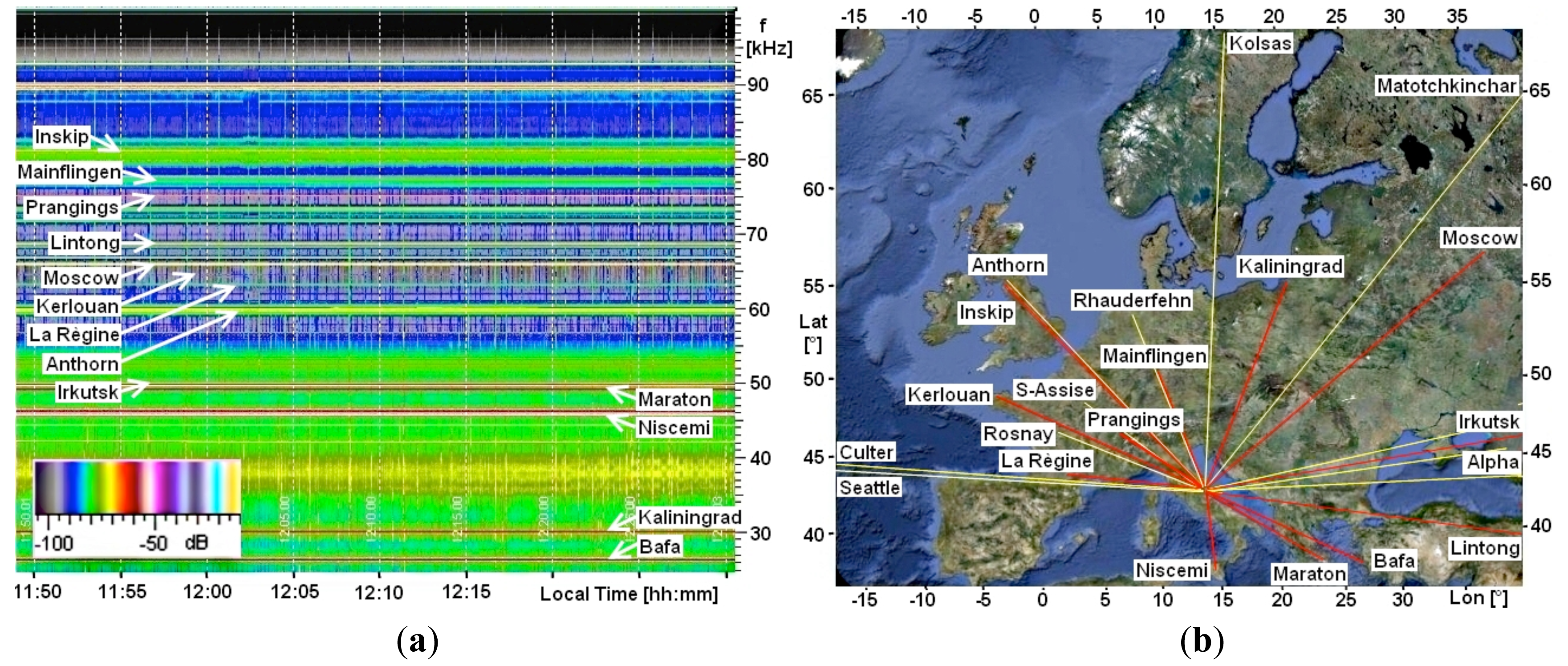
Each station can be composed of multiple receivers tuned to different transmitters so as to monitor sub-ionospheric channels in different directions. A network of stations is thus able to achieve complete monitoring. For this reason, the instrument described here has some inherent advantages. First, as it uses a wide band amplifier, just one instrument permits to observe many transmitters simultaneously. Second, a software solution can be used to separate the different transmitter's signals. To further raise the number of reached transmitters the CIEN, frequency bandwidth was increased to 100 kHz of the LF band. The Chieti Station had already been modified this way and a corresponding LF spectrogram is shown in Figure 7. The set of all sub-ionospheric channels is indicated on the right of Figure 7. The Chieti Station receives LF signals from [35]: Bafa, Turkey, 26.7 kHz; Kaliningrad, Russia, 30.3 kHz; Niscemi, Italy, 45.9 kHz; Maraton, Greece, 49.0 kHz; Irkutsk, Russia, 50.0 kHz; Anthorn, England, 60.0 kHz; La Règine, France, 62.6 kHz; Kerlouan, France, 65.8 kHz; Moscow, Russia, 66.6 kHz; Lintong, China, 68.5 kHz; Prangings, Switzerland, 75.0 kHz; Mainflingen, Germany, 77.5 kHz; Inskip, England, 81.0 kHz; and others not well localized yet.
Several sub-ionospheric signals from different VLF transmitters overlap along the same channels, which is an important feature of a reliable system that is able to verify a single channel perturbation from at least two signals. Additionally, different CIEN stations are able to recognize overlapping along the same direction with the transmitter. This redundancy is necessary for determining the correct functioning of the transmitting stations. Finally, both the multiple signals from different distant transmitters along the same channels and the crossing channels realized by CIEN can also aid in determining the distance of perturbation from the stations, in order to better indicate the critical region.
2.4. ELF and VLF Signatures Related to Meteorological Activity
Rain and thunderstorms strongly influence the ELF band. This is because strong movements of electric charges in the clouds are associated to meteorological perturbations that influence this electric field band [41]. A recording of a thunderstorm above the Capitignano Station is shown in Figure 8. Being that the time evolution moves rightward on the plot, it is possible to see that the arrival of rainfall is associated with an increase in spherics, in both number and intensity. Such increases are determined by lightning bolts and inter-cloud discharges as they approach the station. When rainfall begins at the Capitignano Station, a 30 dB increase in power continuously fills the whole spectrum until the end of rainfall. This is the electrical charge of raindrops falling from thunderclouds [42] and striking the wire antenna. Frequently, the power spectrum amplitude increases to more than 40 dB and polarity of electric perturbations changes during rainfall, as charges can increase with raindrop dimensions and a change in the sign of the charge [42]. The signal amplitude of Figure 8 appeared principally negative during the first five minutes, while it became positive over the subsequent five minutes, initially indicating positively and then negatively charged raindrops, according to inverting amplification. During rainfall, only power supply harmonics remain visible on the spectrum, while other natural signals are hidden by these perturbations. The plot in Figure 8 shows a rare case of oscillations before and/or after rainfall similar to those seen in Figures 3 and 4; even if this almost always comes from a single antenna. These rain-related oscillations usually last no more than five minutes, unlike oscillations recorded before seismic events which can last hours. Such signals were nearly always connected and always near in time to the rainfall shape of the EM spectrum. Furthermore, the oscillations occurring with rainfall usually reach higher frequencies than earthquakes; up to 800 Hz and 400 Hz respectively.
Strong meteorological perturbations can also influence the radio transmissions by refracting the carrier waves; for example this occurred in Perugia on 27 July 2011, in the early afternoon, when an intense rainfall swept the area as shown in Figure 9. These intense rain falls are frequent in this region and sometimes have grave consequences [43]. Finding a method to forecast or mitigate these consequences caused by extreme events is of great interest for the Italian Civil Protection Agency. In the spectrogram plotted on Figure 9, a high intensity rainfall event is associated with ELF band where power increased to 50 dB, whereas, strong signals also appear on the bottom of VLF band. Here, one can observe the surprising disappearance of the signal at 16 kHz at about 16:35LT, which is produced by the photovoltaic power supply and suggesting that the sun was obscured for some minutes by the intense precipitations. During the same time interval the yellow belt fades as do the carrier waves of several transmitters. Given the sun light attenuation it is reasonable to deduce that the strong perturbation was precisely above the Perugia Station. Looking at the dynamical spectrum of Figure 9, one can see another time where several carrier waves are attenuated in amplitude because of strong rainfall, at about 16:03LT. Here there was no interruption of 16 kHz signal, indicating that the sunlight was not obscured. In both cases rain influenced VLF radio propagation near the station. The alpha transmitters did not appear in the spectrograms of that period, however, it is possible verify that they suddenly disappeared some days before and suddenly reappeared some days later. This phenomenon was also recorded at other stations, thereby, suggesting that transmitters must have been switched off during this period and not influenced by meteorology. These anthropogenic and meteorological modulations must be taken in account to identify true earthquake influences.
3. Experimental Settings and Calibration
CIEN instruments are made up of two principal parts: the outdoor sensor and the indoor recording system. The sensor is composed of electrode wires with electronics that prepare the signals. Sensors must be positioned outdoors as they are responsible for picking up EM signals in the atmosphere. The recording system consists of a standard PC audio card with the necessary software to carry out a real time analysis and store data. The recording system is positioned indoors so as to protect it from the weather. The power supply for the sensor electronics is incorporated into the PC, while the indoor and outdoor parts are connected by a multiple signal/power-supply shielded wire. Despite the simplicity of the system, it will be shown in section below that it allows to take quantitative and well suited measurements.
3.1. CIEN Outdoor Antennae
All antennae have two long thin wires, from l = 10 m to l = 20 m in length and from s = 0.5 mm to s = 1 mm of thickness, which are perpendicular to each other and horizontally fixed at about h = 8–10 m off the ground. These are positioned at the eight CIEN stations, indicated in Table 1, together with their coordinates and features. All the station electrodes have one wire positioned approximately toward the N-S and the other wire toward the E-W. The wires are covered by an insulating sheath as well the supports that keep them off the ground. Moreover, all conductive parts of the system are also covered by an insulating sheath to protect against direct contact with atmospheric charge, while the mass supply is connected to ground. The electronics include two amplifiers having high impedance, high gain and wide band (DC to 100 kHz). Finally, a protection limits excessive induced electrical potentials on the electrodes, thereby preventing damage to the electronics.
The two floating wires behave like very short antennas in ELF, VLF and LF bands [44], as they are two monopoles perpendicular to each other and parallel to the ground. Being LF, they have wavelengths much longer than the CIEN monopoles. Though the antenna gain is very low, it can be recovered by using a long wire antenna [44]. Capacitive effect inductions of wires with respect to the ground become comparable in amplitude to the electric field horizontal line inductions. A relationship between the capacitive vertical field induced potential and the horizontal field summation along the antenna can be calculated. To quantify the electromagnetic inductions on these electrodes it is necessary to consider the monopole theory at such low frequencies as seen here.
Referring to antenna theory, one is reminded that the relative pattern of a horizontal monopole above a lossy surface is not significantly different from that which is above a perfect conductor [45]. Being so, one can consider these results in this simple case. Moreover, as these frequencies are less than 100 kHz, the wavelength λ is always longer than 3 km. Indeed, for the ELF band, λ is longer than 1,000 km; thus l ≪ λ. In this case, being that h ≪ λ, the antenna directivity gain is not any longer a function of its height [45]. Therefore, assuming constant electric field along the wire dimension, the induced potential is defined as a scalar product l·E; where l is the effective length parameter of the monopole, while E is the total electric field incident on the wires [44]. As the current intensity is constant in a small monopole with l ≪ λ [45], the effective length parameter will be equal to the monopole length l and the open-circuit voltage va can be approximately written as
Two perpendicular antennas can be used to reconstruct the polarization state of the electric field, which can be represented by the polarization ellipse and described mathematically by the four Stokes parameters [46]. Writing the components of E as
If Z is the intrinsic vacuum impedance, the Stokes parameters are
Vertical electric fields also induce identical potentials onto the wires which depend on their height and capacity with respect to the ground. Under the hypotheses that the vertical electric field Ev is constant moving vertically at the altitude h ≪ λ, the induced terminal voltage vc is [47]
The presence of a conductive ground produces reflections of EM waves producing a mismatched sum of directed and reflected waves at the antenna position. The wire system can be studied using the image method, which affirms that an equal and opposite current runs underground. The reflected wave is therefore characterized by an opposite horizontal electric field that subtracts its contribution from the directed electric field wave. The difference between the opposite fields only depends on a phase factor which is linked to the height of the antenna [44], which is near zero for long waves with h ≪ λ. Moreover, the confinement of the field between the ground and the ionosphere provides a very stable propagation path, where the length of ELF propagation is only compatible with the quasi-transverse EM mode [44]. Being so, plane ELF waves such as Schumann Resonances or spherics can only be vertical fields. Instead, in the VLF range above 10 kHz, the guide height is several wavelengths in dimension, thus allowing for many propagation modes [44].
3.2. CIEN Recording System and Its Calibration
Sensors are connected to a PC at each station which supplies power to the electronics and samples the signals by way of sound cards. The signals are registered in stereo mode for both direction antennas with a 16 bit A/D conversion, permitting a dynamical range of about 96 dB. This is necessary, as weak signals start at −100 dB, while meteorological perturbations can increase the signal amplitudes up until −20 dB. Spectrum Laboratory free software [48] is used to fix the recording parameters and to analyze the signals utilizing Fast Fourier Transform (FFT). Data is stored in DVD for further analysis allowing for a further comparison of the measurements. The wave files here would have taken up too much memory space; they are therefore compressed lossless by another free algorithm [49].
Given that these compressed wave recordings also occupy much space they are only active for the ELF band. Signals are sampled through a frequency of 2 kHz, so to have a Nyquist frequency which allows perfect reconstruction of the signal bandwidth up to 1 kHz [50]. Minimum frequency detection depends on both sound card type and quality. As described below here, this frequency usually reaches 1 Hz by utilising active digital filters and evaluating system noise amplitude. The ULF band can be reached by utilising high quality sound cards, which reduce noise and allow us to discriminate between the signals below Hz. In the VLF and LF bands, time evolution signals are recorded on the transmitter power frequencies. In these bands, the carrier wave peak amplitudes and the phases are measured every five minutes.
FFT analysis is performed on all bands and one spectrogram is saved for each band in compressed jpeg image. FFT is calculated for both the channels at every 4.096 seconds with an input size of 16,384 and a Hann window function. The power amplitude range was chosen to cover −106 dB to −10 dB with the to many colors legend, which allows us to distinguish about 20 different colors and shades, permitting to evaluate 5 dB amplitude differences. Color images were saved with a resolution of 1,278 × 972 pixels. Different frequency scales were used to plot the bands so as to better present the spectrograms plotted in all the figures, a logarithm scale was used for ULF and ELF bands, whereas a linear scale was used for the VLF and LF bands. Time was identified on the spectrograms by white dashed vertical lines, one every 300 seconds.
A quantitative amplitude estimation of some previously observed signals requires calibration, as we do not know all the signal transfer functions which occur in this system. This calibration can be realized in different ways, taking into account electromagnetic theory as well as experimental methods. Above all, the band pass transfer functions T(ω) = Ta(ω) × Ts(ω), product of the audio sound card transfer Ta(ω) and the sensor amplifier transfer Ts(ω) functions, should be experimentally determined. This can be obtained through a wave generator and an oscilloscope which are connected at the input and output of these electronics, respectively. Thus, the theory in the Section 3.1 can be used to calculate the electric field at the antenna positions. The true potential on the wire can now be written as
Having wave recordings, it has been possible to further analyze the signals by Spectrum Laboratory software, after changing several possible parameters of FFT calculus and visualization. Being so, some specific weak signals including Schumann Resonances are better evidenced. But, in order to increase analysis quality, software specifically developed for audio signal processing has been utilized. Through FFT analysis, all digital operations on the signals have been possible, including background noise reduction, filtering and signal isolation. As an example, one can consider the electric signal in Figure 4. In this case, an active filter with precise transfer function that compensates for electronics band pass can be introduced by the Audacity software [51]. After this, a region where the oscillation disappears is selected and its power spectrum content is calculated as a noise. Moreover, the Audacity software performs a digital FFT subtraction of the noise from FFT signals and FFTs it into a new wave file. The new file contains the isolated electric oscillation which is shown together with the amplitudes before and after the operation in Figure 10. An audio file reproduction from 7:48:20 to 7:51:20 of the filtered signal in Figure 10, which sounds like a soft hiss, is available in the supplementary material.
Given this, a comparison between well-known natural signals of fixed frequencies and the corresponding power spectrum which are near the same frequencies can be used to calibrate the instrument in that particular range. At this point, the amplitudes of the oscillations in Figures 3 and 4 can be evaluated by comparing them to the Schumann Resonances by utilizing (8). On a non-electrically perturbed day, Schumann Resonances are usually well above the noise level, and can be detected in a section of the spectrogram, as shown in the middle of three parts in Figure 11. The transfer function T−1(ω) in Figure 10, is applied to compensate for the low frequency attenuation using the Audacity software on the wave file corresponding to the spectrogram on the left in Figure 11. The resulting power spectrum is plotted on the right in Figure 11, with the correct power spectrum associated to each natural resonance electric field amplitude. In this way, with a set of well-known amplitude points in the spectrum, it is possible calibrate the whole range. The electric field amplitudes of the Schumann Resonances reach 0.1 mV/m and are vertical fields [33], being so, they can be expressed by (7) and produce |vc| = 7.8 μV for the first Resonance.
To evaluate the amplitudes of the oscillations it is important to remember that they almost always appear on one wire, thereby confirming the prevalent horizontal direction of electric fields. However, in some cases a component in the other horizontal and vertical directions appears. The spectrogram color legend permits us to distinguish not less than 5 dB amplitude differences. This means that it is able to evaluate a factor 2, which is not very precise. On the other hand, noise level can reduce sensibility to small components of the oscillation on the other wire. This is because the signal amplitude is in some cases only 5–10 dB above the noise. When measured with precision, the Stokes parameters defined in (3), (4), (5) and (6) are useful for detecting partial polarizations, but the method for subtracting the noise described above must be used to obtain accurate results. Here, the signals shown in Figures 3, 4 and 11 are more than 20 db above the noise and the noise subtraction is not necessary as the other component results being at least 10 times smaller. To compare vertical and horizontal inductions on the wires (1), (7) as well as the difference between the first Schumann Resonance and the oscillation in dB are used. These produce amplitudes corresponding to 3.5 μV for signals in Figure 11, and about 35 μV for signals in Figures 3 and 4; which correspond to electric field intensities of 0.17 μV/m and 1.7 μV/m respectively. With Perugia Station wires of l = 20 m, h = 10 m, r = 0.5 mm, εr = 1, so that C = 105 pF; where ω = 7.4 Hz, Ri = 10 MΩ, Ev = 0.1 mV/m and |vc| > |va| of 7 dB.
Finally, some attempts were made to explain the possible field sources through the characteristics of the signals. The single oscillations were uncorrelated in time among the CIEN stations, although, a general recurrence of oscillations was observed over identical periods on many occasions. Furthermore, oscillations were rarely observed simultaneously from different wires of the same station and always these simultaneous signals are of different spectral shapes, intensities and durations while their frequencies are similar. For these reasons, a series of experiments were performed to determine if these signals had been created inside the electronics. The two wires of a single sensor were initially positioned close to and parallel to each other, verifying that oscillations appeared on both wires. Afterwards, a new sensor with slightly different wire lengths and input impedances was used, and was connected to a different PC with a different power supply. Wires of this new sensor were not perpendicular to each other. Instead, one was positioned parallel and close to a wire of the old instrument, while the other wire was positioned at an odd angle with all four wires being at the same height. The same signals reappeared only on the parallel wires, even if they had different amplitudes due to their different lengths. A third sensor was positioned at the station but its wires were not positioned perpendicular to any of the other wires. This was done in order to monitor signals from different angles; all wires were at the same height. Electronics without wires were also studied but no electric oscillations were observed. From this, it can be concluded that the oscillations were not created by electronics but were induced by principal horizontal polarizations of electric components. Furthermore, missing correlations between signals at different stations far apart less than 50–100 km suggested the presence of local electric field perturbations with sources distances less than 50 km. Given their characteristics, these signals may have been different from those measured by satellites [30]. The local nature of the electric oscillations suggests that the activities do occur during the stress build-up in the focal area of large and shallow earthquakes [23].
4. Conclusions
This study of data from eight CIEN stations suggests that electric perturbations become more intense during seismically intense periods, and their powers become greater than other natural EM phenomena, such as the Schumann Resonances. Candidate pre-seismic oscillations in electric amplitudes were quantified allowing for the verification of some hypotheses regarding observed phenomena [52–56]. These oscillations are well discriminated from other natural and anthropogenic signals in spectrograms, whenever meteorological events, primarily thunderstorms and heavy rain, are far away from the stations. Their characteristics include the following:
frequencies in ELF band from 20 Hz to 400 Hz, seldom starting and ending at lower frequencies;
frequencies ranging from 10 Hz to 100 Hz, with multiple structures in some intense cases;
intensities greater than 1 μV/m during seismic activity with M ≥ 5;
strongest intensities during seismically intense periods;
duration from several minutes to some hours;
mostly horizontally polarized;
local <50 km sources;
similar but briefer perturbations at higher frequency before intense rainfall.
Figure 3 shows the signals a few minutes after the L'Aquila main shock. They appeared several minutes after the passage of the seismic wave at the Perugia Station, indicating that it was niether a co-seismic nor a “co-seismic wave” phenomenon [23]. In the laboratory EM emissions were observed in the range from kHz to MHz [57], whereas, the signals shown in Figures 3, 4 and 7 were in the range from tens of Hz to hundreds of Hz. The similarity between laboratory acoustic emissions, which occur at frequencies between 50–800 kHz, and seismic activity is well accepted [58], with wave frequencies ranging between 1–30 Hz. The frequency ratio between laboratory and natural cases is more than 104 for both acoustic and EM emissions, which is also the ratio between laboratory samples and earthquake fault dimensions. However, contrarily to the cases discussed here EM emissions in the laboratory were observed through their magnetic components only in correspondence to the sharp stress drops in the load versus time diagrams, independently of the materials [59]. Furthermore, the geological composition of the Earth surface and the presence of water in the Earth surface/air interface strongly modulates the amplitude and the shape of electric signals.
Characteristic (8) above suggests a further interpretation as electric charging of the air has been frequently reported to precede meteorological perturbations [60]. Specifically, charged aerosols in the air could have some links with the observed electric oscillations [61]. Air ionization has been identified at rock surfaces [53] and gas emission can be a charge carrier [62]. Thus, the link between these EM signals and earthquakes could also be indirect and mediated by other processes. Figure 5 shows that strong electric oscillations also occurred during the aftershock period. This is in agreement with other EM signals recorded near other focal areas, which show a prolonged EM activity during the main shock [23]. Moreover, the long-term monitoring of some gas vents in Central Italy showed a significant set of anomalies that had durations of several weeks after the main shock [63]. Figure 5 shows this type of electric perturbation to have its maximum value in correspondence with VLF [64] and IR [65] anomalies which appeared some days prior to the main shock.
CIEN has been designed to record ELF band data so as to thoroughly analyze these data and compare them to other measurements. This analysis can benefit from advanced audio signal software for reducing noise and isolating particular EM phenomena. CIEN sensors are a broad band system which allows us to extend the monitoring of ULF, VLF and LF bands. Above 10 kHz, VLF and LF radio transmitter carrier wave intensities are collected to monitor about 20 sub-ionospheric channels, and verify perturbations whenever strong earthquakes occur under their path. ULF monitoring has just begun and therefore it is in an experimental stage.
Strong meteorological perturbations have also shown many intense electric signals in all the bands monitored by CIEN. The ELF band mirrors rainfall providing us with an alternative way of monitoring rainfall by means of electric intensity perturbations. The VLF and LF bands have also shown some radio shadowing effects of transmitters, which could be used to further investigate rainfall around stations and to improve upon standard rain gauges. Finally, the spectrogram representation of natural and anthropogenic electric signals provides a simple and intuitive way of discovering a world otherwise unseen. Thus, as already proposed [66], this approach may have interesting educational applications for high school and undergraduate level experiments, since only simple instrumentation is required.


| Station | Latitude | Longitude | Altitude | Frequency Bands | Services | Other Instruments |
|---|---|---|---|---|---|---|
| Fermo | 43°04′08″ | 13°56′58″ | 200 m | ELF, VLF | Web | - |
| Perugia | 43°07′13″ | 12°23′12″ | 460 m | ELF, VLF | Web | SS |
| Zocca | 44°21′21″ | 10°59′29″ | 750 m | ELF, VLF | UPS | - |
| Capitignano | 42°31′59″ | 13°17′27″ | 920 m | ELF, VLF | - | - |
| Chieti | 42°22′05″ | 14°08′52″ | 60 m | ULF, ELF, VLF, LF | Web, UPS | AC, MG, PF |
| Siena | 43°18′52″ | 11°19′20″ | 320 m | ELF, VLF | Web | - |
| Fagnano | 42°15′57″ | 13°35′01″ | 710 m | ELF, VLF | Web | RD, SS |
| Rieti | 42°24′37″ | 12°46′10″ | 430 m | ELF, VLF | Web | LC, SS |
Acknowledgments
The Author would like to gratefully thank those who have hosted and contributed to building the CIEN stations: Francesco Stoppa, Dario Albarello, Giovanni Martinelli, Andrea Vannucchi, Giovanni Iezzi, Mirta Morrone, Angelo Zaroli, Paolo Antonio Salvadori, Giampaolo Giuliani, Leonardo Nicolì and Diego Valeri. Thanks for suggestions to Friedemann T. Freund, Mohammed Y. Boudjada, Maria Teresa Brunetti, Michele Arcaleni, Wolfgang “Wolf” Buescher and anonymous referees, who suggested adding the similarity between EM and acoustic emissions. Furthermore, the Author would like to thank the following for offering their PC hardware solutions: Giovanna De Liso and “Le Nuove Muse” association, Hassen Riahi, Stefano Lince, Physics and Institutions and Society Departments of Perugia University and Foto Digital Discount Bianchi in Via della Pallotta, Perugia.
References
- Serpieri, A. Sullo studio della perturbazione elettrica foriera del terremoto. Riv. Sci.-Ind. 1874, 6, 165–173. [Google Scholar]
- Serpieri, A. Elettricità e terremoto. Rendiconti Istituto Lombardo Scienze Lettere 1880, 13, 193–194. [Google Scholar]
- Baratta, M. Catalogo dei fenomeni elettrici e magnetici apparsi durante i principali terremoti. In Rendiconti della Società Italiana di Elettricità pel progresso degli studi e delle applicazioni; Tip. Lamperti di G. Rozza: Milan, Italy, 1891; 1-anno XIII; pp. 1–15. [Google Scholar]
- Fidani, C. Ipotesi Sulle Anomalie Elettromagnetiche Associate ai Terremoti, 1st ed.; Libreria Universitaria Benedetti L'Aquila: L'Aquila, Italy, 2005; p. 300. [Google Scholar]
- Palmieri, L. Sulle Scoperte Vesuviane Attenenti Alla Elettricità Atmosferica: Disquisizioni Accademiche; Stabilimento tipografico de G. Nobile: Napoli, Italy, 1854; p. 33. [Google Scholar]
- Calzecchi-Onesti, T. Di una nuova forma che può darsi all'avvisatore microsismico. Nuovo Cimento 1886, XIX, 24–26. [Google Scholar]
- Maccioni, P.A. Nuova scoperta nel campo della sismologia. Atti della R. Accademia dei Fisiocritici 1909, I, 435–444. [Google Scholar]
- Ungania, E. Presismofono Ungania Unico Apparecchio Preavvisatore dei Terremoti; Tipografia Luigi Parma: Bologna, Italy, 1924; p. 34. [Google Scholar]
- Fidani, C. On Electromagnetic precursors of earth-quakes: Models and instruments. Proceedings of IPHW, Bologna, Italy, 17 June 2005; pp. 25–41.
- Jondral, F.K. From Maxwell's equations to cognitive radio. Proceedings of the 3rd International Conference on Cognitive Radio Oriented Wireless Networks and Communications, CrownCom, Singapore, 15–17 May 2008; pp. 1–5.
- Kant, I. Geschichte und Naturbeschreibung der merkwürdigsten Vorfälle des Erdbebens, welches an dem Ende des 1775sten Jahres einen großen Teil der Erde erschüttert hat, 1776. In Kant's Werke I; Akademie-Textausgabe: Berlin, Germany, 1968; pp. 429–462. [Google Scholar]
- Enemoto, Y. Ground electrification anomaly: Is it a precursor of large earthquake occurrence? Highlight of physics at edo-age on relationship between ‘Elektriciteit’ and earthquakes. J. Surf. Sci. Soc. Jpn. 2002, 23, 56–61. [Google Scholar]
- Rikitake, T.; Honkura, Y.; Tanaka, H.; Ohshiman, N.; Sasai, Y.; Ishikawa, Y.; Koyama, S.; Kawamura, M.; Ohchi, K. Changes in the geomagnetic field associated with earthquakes in the Izu Peninsula, Japan. J. Geomag. Geoelectr. 1980, 32, 721–739. [Google Scholar]
- Rikitake, T. Geomagnetism and earthquake prediction. Tectonophysics 1968, 6, 59–68. [Google Scholar]
- Moore, G.W. Magnetic disturbances preceding the 1964 Alaska earthquakes. Nature 1964, 203, 508–509. [Google Scholar]
- Breiner, S.; Kovach, R.L. Local geomagnetic events associated with displacements on the San Andreas Fault. Science 1967, 158, 116–118. [Google Scholar]
- Thomas, J.N.; Love, J.J.; Johnston, M.J.S. On the reported magnetic precursor of the 1989 Loma Prieta earthquake. Phys. Earth Planet. Inter. 2009, 173, 207–215. [Google Scholar]
- Thomas, J.N.; Love, J.J.; Johnston, M.J.S.; Yumoto, K. On the reported magnetic precursor of the 1993 Guam earthquake. Geophys. Res. Lett. 2009, 36, L16301:1–L16301:5. [Google Scholar]
- Villante, U.; Francia, P.; Vellante, M. Long period magnetospheric oscillations at discrete frequencies: The results of a multi-station analysis. Adv. Space Res. 2010, 46, 460–467. [Google Scholar]
- Orsini, M. Electromagnetic anomalies recorded before the earthquake of L'Aquila on April 6, 2009. Bollettino di Geofisica Teorica ed Applicata 2011, 52, 123–130. [Google Scholar]
- Bleier, T.E.; Dunson, C.; Maniscalco, M.; Bryant, N.; Bambery, R.; Freund, F. Investigation of ULF magnetic pulsations, air conductivity changes, and infra red signatures associated with the 30 October Alum Rock M5.4 earthquake. Nat. Hazards Earth Syst. Sci. 2009, 9, 585–603. [Google Scholar]
- Dunson, J.C.; Bleier, T.E.; Roth, S.; Heraud, J.; Alvarez, C.H.; Lira, A. The Pulse Azimuth effect as seen in induction coil magnetometers located in California and Peru 2007–2010, and its possible association with earthquakes. Nat. Hazards Earth Syst. Sci. 2011, 11, 2085–2105. [Google Scholar]
- Uyeda, S.; Nagao, T.; Kamogawa, M. Short-term earthquake prediction: Current status of seismo-electromagnetics. Tectonophysics 2009, 470, 205–213. [Google Scholar]
- Bina, A. Ragionamento Sopra la Cagione de Terremoti; Abbazia di San Pietro: Perugia, Italy, 1751. [Google Scholar]
- Beccaria, G.B. Lettere dell'elettricismo; Colle Ameno Editore: Bologna, Italy, 1754. [Google Scholar]
- Volta, A. Memoria. Sopra i Fuochi de' Terreni e delle Fontane ardenti in generale, e sopra quelli di Pietra-Mala in particolare. Memorie di matematica e di fisica della Società Italiana 1784, tomo II, 662–665. [Google Scholar]
- Vannucci, G. Discorso Istorico Filosofico sopra il tremuoto del 25 dicembre 1786; Cesena, Italy, 1787. [Google Scholar]
- Galli, I. Raccolta e classificazione dei fenomeni luminosi osservati nei terremoti. Bollettino della Società Sismologica Italiana 1910, 14, 221–448. [Google Scholar]
- Biagi, P.F.; Maggipinto, T.; Righetti, F.; Loiacono, D.; Schiavulli, L.; Ligonzo, T.; Ermini, A.; Moldovan, I.A.; Moldovan, A.S.; Buyuksarac, A.; Silva, H.G.; Bezzeghoud, M.; Contadakis, M.E. The European VLF/LF radio network to search for earthquake precursors: Setting up and natural/man-made disturbances. Nat. Hazards Earth Syst. Sci. 2011, 11, 333–341. [Google Scholar]
- Parrot, M. Anomalous seismic phenomena view from space. In Electromagnetic Phenomena Associated with Earthquakes; Hayakawa, M., Ed.; Transworld Research Network: Tokyo, Japan, 2010; pp. 205–233. [Google Scholar]
- Google Maps™ Servizio Generazione Mappe; Google Italy: Milan, Italy, 2011. Available online: http://maps.google.it/ (accessed on 1 November 2011).
- Barr, R.; Jones, D.L.; Rodger, C.J. ELF and VLF radio waves. J. Atmos. Solar-Terr. Phys. 2000, 62, 1689–1718. [Google Scholar]
- Jackson, J.D. Classical Electrodynamics, 1st ed.; Wiley and Sons Inc.: Hoboken, NJ, USA, 1975; p. 363. [Google Scholar]
- Cummer, S.A. Modeling electromagnetic propagation in the earth-ionosphere waveguide. IEEE Trans. Antennas Propag. 2000, 48, 1420–1430. [Google Scholar]
- Lionel LOUDET. VLF Stations List; STD Monitoring Station: France, 2011. Available online: http://sidstation.loudet.org/stations-list-en.xhtml (accessed on 1 November 2011).
- Fidani, C. ELF Signals by Central Italy electromagnetic network in 2008–2010. Proceedings of Atti del 29 GNGTS, Prato, Italy, 28–30 October 2010; pp. 175–179.
- Bindi, D.; Pacor, F.; Luzi, L.; Massa, M.; Ameri, G. The Mw = 6.3, 2009 L'Aquila earthquake: Source, path and site effects from spectral analysis of strong motion data. Geophys. J. Int. 2009, 179, 1573–1579. [Google Scholar]
- Fidani, C. Electromagnetic signals recorded by Perugia and S. Procolo (Fermo) stations before the L'Aquila Earthquakes. Proceedings of Atti del 28 GNGTS, Trieste, Italy, 16–19 November 2009; pp. 370–373.
- Dobrovolsky, I.P.; Zubkov, S.I.; Miachkin, V.I. Estimation of the size of earthquake preparation zones. Pure Appl. Geophys. 1979, 117, 1025–1044. [Google Scholar]
- Hayakawa, M.; Molchanov, O.A.; Ondoh, T.; Kawai, E. Anomalies in the sub-ionospheric VLF signals for the 1995 Hyogo-Ken Nambu earthquake. J. Phys. Earth 1996, 44, 413–418. [Google Scholar]
- Singh, D.; Singh, A.K.; Patel, R.P.; Singh, R.; Singh, R.P.; Veenadhari, B.; Mukherjee, M. Thunderstorms, lightning, sprites and magnetospheric whistler-mode radio waves. Surv. Geophys. 2008, 29, 499–551. [Google Scholar]
- Gunn, R. The free electrical charge on thunderstorm rain and its relation to droplet size. J. Geophys. Res. 1949, 54, 57–63. [Google Scholar]
- Weather Extremes in a Changing Climate: Hindsight on Foresight; World Meteorological Organization: Geneva, Switzerland, 2011. WMO-No. 1075. Available online: http://www.wmo.int/pages/mediacentre/news/documents/1075_en.pdf (accessed on 1 November 2011).
- Colin, R.E. Antennas and Radiowave Propagation, International Student ed.; McGraw-Hill series in Electrical Engineering: New York, NY, USA, 1985; p. 508. [Google Scholar]
- Balanis, C.A. Antenna Theory, 2nd ed.; Wiley and Sons Inc.: Hoboken, NJ, USA, 1982; p. 941. [Google Scholar]
- Sawas, S.; Boudjada, M.Y.; Lecacheux, A.; Stangl, A.; Rucker, H.O.; Voller, W. Interactive Software for Spectral Analysis (ISSA): Cases of The Digital Spectro-Polarimeter and the Spectro-Analyzer Receivers; Report of the Space Research Institute; Austrian Academy of Sciences: Vienna, Austrian, 2003; Volume 141, pp. 20–31. [Google Scholar]
- Roy, A.; Ghosh, S.; Chakrabarty, A. Simple susceptibility model of two wires to predict EM wave pickup in an EMI/EMC environment. Proceedings of IEEE Applied Electromagnetics Conference, Kolkata, Indian, 19–20 December 2007; EMI 01. pp. 1–4.
- DL4YHF's Amateur Radio Software: Audio Spectrum Analyzer (“Spectrum Lab”) 2.76, 2011. DL4YHF Home Page. Available online: http://www.qsl.net/dl4yhf/spectra1.html (accessed on 1 November 2011).
- Lossless Audio Compression Version 0.4b; Michael Bevin, February 2004. Lossless Audio Home Page. Available online: http://www.lossless-audio.com/index.htm (accessed on 1 November 2011).
- Grenander, U. The Nyquist Frequency is that frequency whose period is two sampling intervals. In Probability and Statistics: The Harald Cramér Volume; John Wiley & Sons: San Francisco, CA, USA, 1959; p. 434. [Google Scholar]
- Audacity 1.2.6; Dominic Mazzoni: Santa Monica, CA, USA, 2011. Available online: http://audacity.sourceforge.net/ (accessed on 1 November 2011).
- Grant, R.A.; Halliday, T. Predicting the unpredictable: Evidence of pre-seismic anticipatory behavior in the common toad. J. Zool. 2010, 281, 263–271. [Google Scholar]
- Freund, F.T.; Kulahci, I.G.; Cyr, G.; Ling, J.; Winnick, M.; Tregloan-Reed, J.; Freund, M.M. Air ionization at rock surface sand pre-earthquake signals. J. Atmos. Solar-Terr. Phys. 2009, 71, 1824–1834. [Google Scholar]
- Grant, R.A.; Halliday, T.; Balderer, W.P.; Leuenberger, F.; Newcomer, M.; Cyr, G.; Freund, F.T. Ground water chemistry changes before major earthquakes and possible effects on animals. Int. J. Environ. Res. Public Health 2011, 8, 1936–1956. [Google Scholar]
- Pulinets, S.; Ouzounov, D. Lithosphere-Atmosphere-Ionosphere Coupling (LAIC) model—An unified concept for earthquake precursors validation. J. Asian Earth Sci. 2011, 41, 371–382. [Google Scholar]
- Ampferer, M.; Denisenko, V.V.; Hausleitner, W.; Krauss, S.; Stangl, G.; Boudjada, M.Y.; Biernat, H.K. Decrease of the electric field penetration into the ionosphere due to low conductivity at the near ground atmospheric layer. Ann. Geophys. 2010, 28, 779–787. [Google Scholar]
- Carpinteri, A.; Lacidogna, G.; Manuello, A.; Niccolini, G.; Schiavi, A.; Agosto, A. Mechanical and electromagnetic emissions related to stress-induced cracks. Exp. Tech. 2011. [Google Scholar] [CrossRef]
- Scholz, C.H. The frequency-magnitude relation of micro fracturing in rock and its relation to earthquakes. Bull. Seismol. Soc. Am. 1968, 58, 399–415. [Google Scholar]
- Lacidogna, G.; Carpinteri, A.; Manuello, A.; Durin, G.; Schiavi, A.; Niccolini, G.; Agosto, A. Acoustic ad electromagnetic emissions as precursor phenomena in failure processes. Strain 2010. [Google Scholar] [CrossRef]
- Takahashi, T. Electric charge of small particles (1–40μ). J. Atmos. Sci. 1972, 29, 921–930. [Google Scholar]
- Tributsch, H. Do aerosol anomalies precede earthquake? Nature 1978, 276, 606–608. [Google Scholar]
- Scudiero, L.; Dickinson, J.T.; Enomoto, Y. The electrification of flowing gases by mechanical abrasion of mineral surfaces. Phys. Chem. Miner. 1998, 25, 566–573. [Google Scholar]
- Heinicke, J.; Martinelli, G.; Telesca, L. Geodynamically induced variations in the emission of CO2 gas at San Faustino (Central Apennines, Italy). Geofluids 2011. [Google Scholar] [CrossRef]
- Rozhnoi, A.; Solovieva, M.; Molchanov, O.; Schwingenschuh, K.; Boudjada, M.; Biagi, P.F.; Maggipinto, T.; Castellana, L.; Ermini, A.; Hayakawa, M. Anomalies in VLF radio signals prior the Abruzzo earthquake (M = 6.3) on 6 April 2009. Nat. Hazards Earth Syst. Sci. 2009, 9, 1727–1732. [Google Scholar]
- Genzano, N.; Aliano, C.; Corrado, R.; Filizzola, C.; Lisi, M.; Mazzeo, G.; Paciello, R.; Pergola, N.; Tramutoli, V. RST analysis of MSG-SEVIRI TIR radiances at the time of the Abruzzo 6 April 2009 earthquake. Nat. Hazards Earth Syst. Sci. 2009, 9, 2073–2084. [Google Scholar]
- Scherrer, D.; Cohen, M.; Hoeksema, T.; Inan, U.; Mitchell, R.; Scherrer, P. Distributing space weather monitoring instruments and educational materials worldwide for IHY 2007: The AWESOME and SID project. Adv. Space Res. 2008, 42, 1777–1785. [Google Scholar]
© 2012 by the authors; licensee MDPI, Basel, Switzerland. This article is an open access article distributed under the terms and conditions of the Creative Commons Attribution license (http://creativecommons.org/licenses/by/3.0/).
Share and Cite
Fidani, C. The Central Italy Electromagnetic Network and the 2009 L'Aquila Earthquake: Observed Electric Activity. Geosciences 2011, 1, 3-25. https://doi.org/10.3390/geosciences1010003
Fidani C. The Central Italy Electromagnetic Network and the 2009 L'Aquila Earthquake: Observed Electric Activity. Geosciences. 2011; 1(1):3-25. https://doi.org/10.3390/geosciences1010003
Chicago/Turabian StyleFidani, Cristiano. 2011. "The Central Italy Electromagnetic Network and the 2009 L'Aquila Earthquake: Observed Electric Activity" Geosciences 1, no. 1: 3-25. https://doi.org/10.3390/geosciences1010003