Examining Local Climate Variability in the Late Pennsylvanian Through Paleosols: An Example from the Lower Conemaugh Group of Southeastern Ohio, USA

Abstract
:1. Introduction
2. Geologic Setting
3. Methods


4. Paleopedology
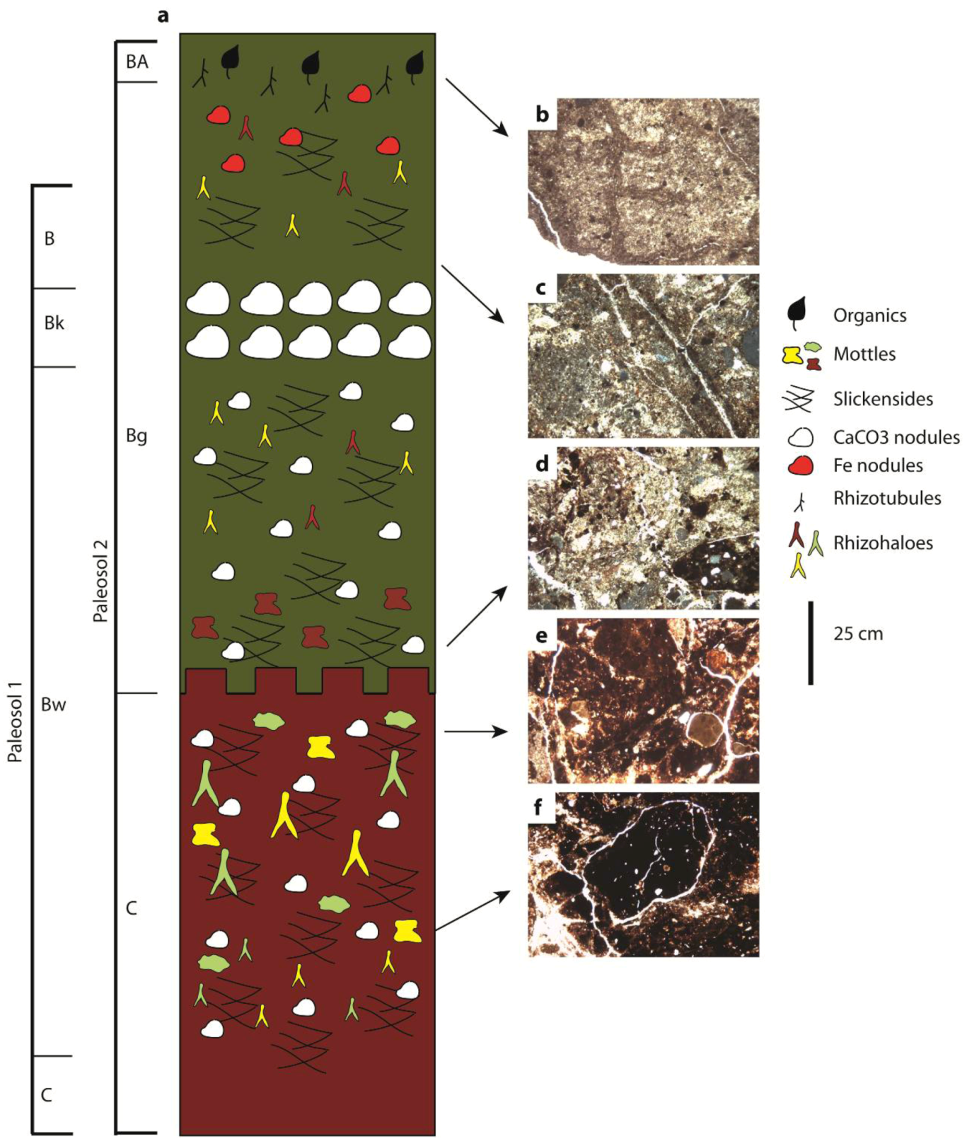
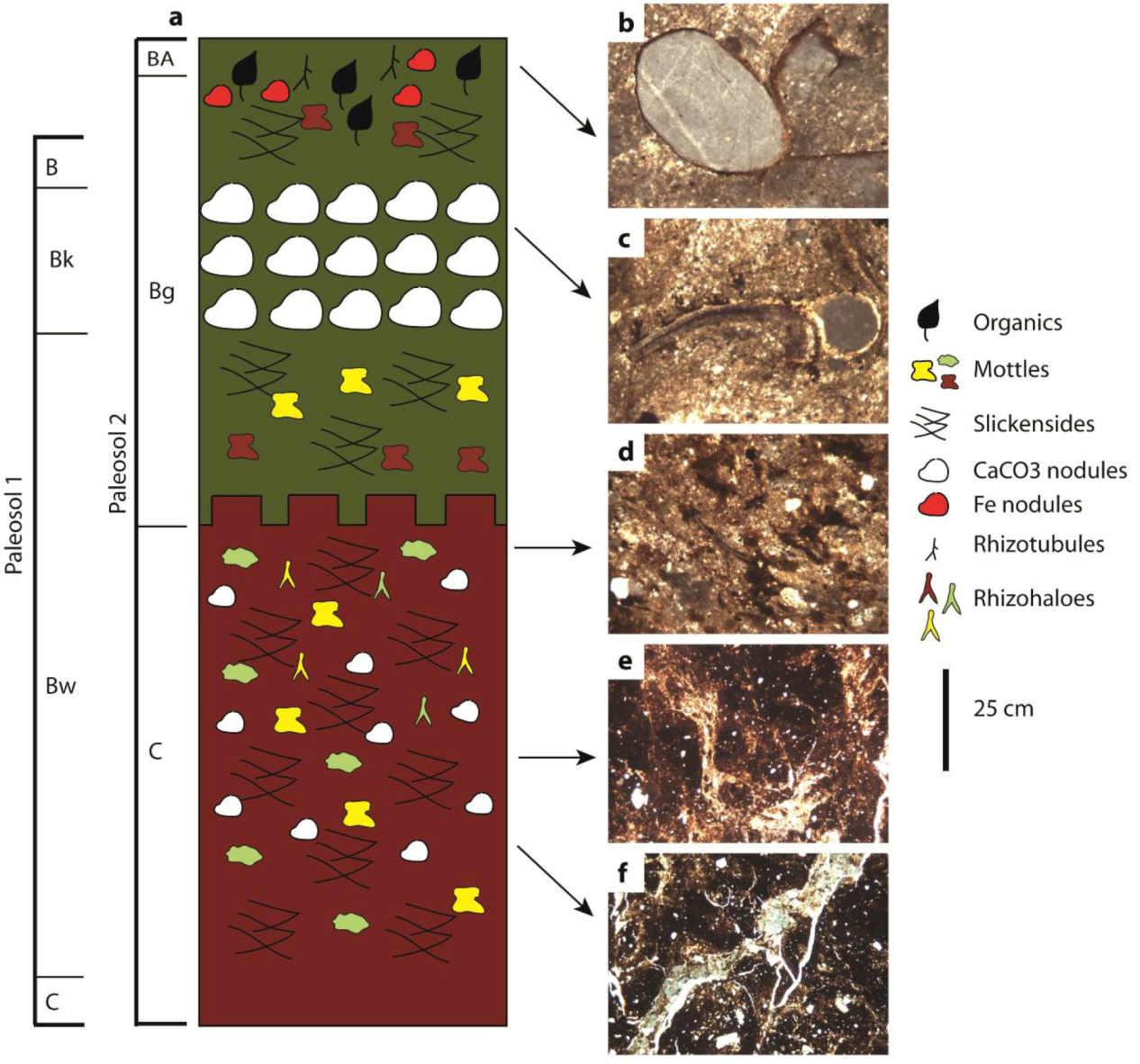
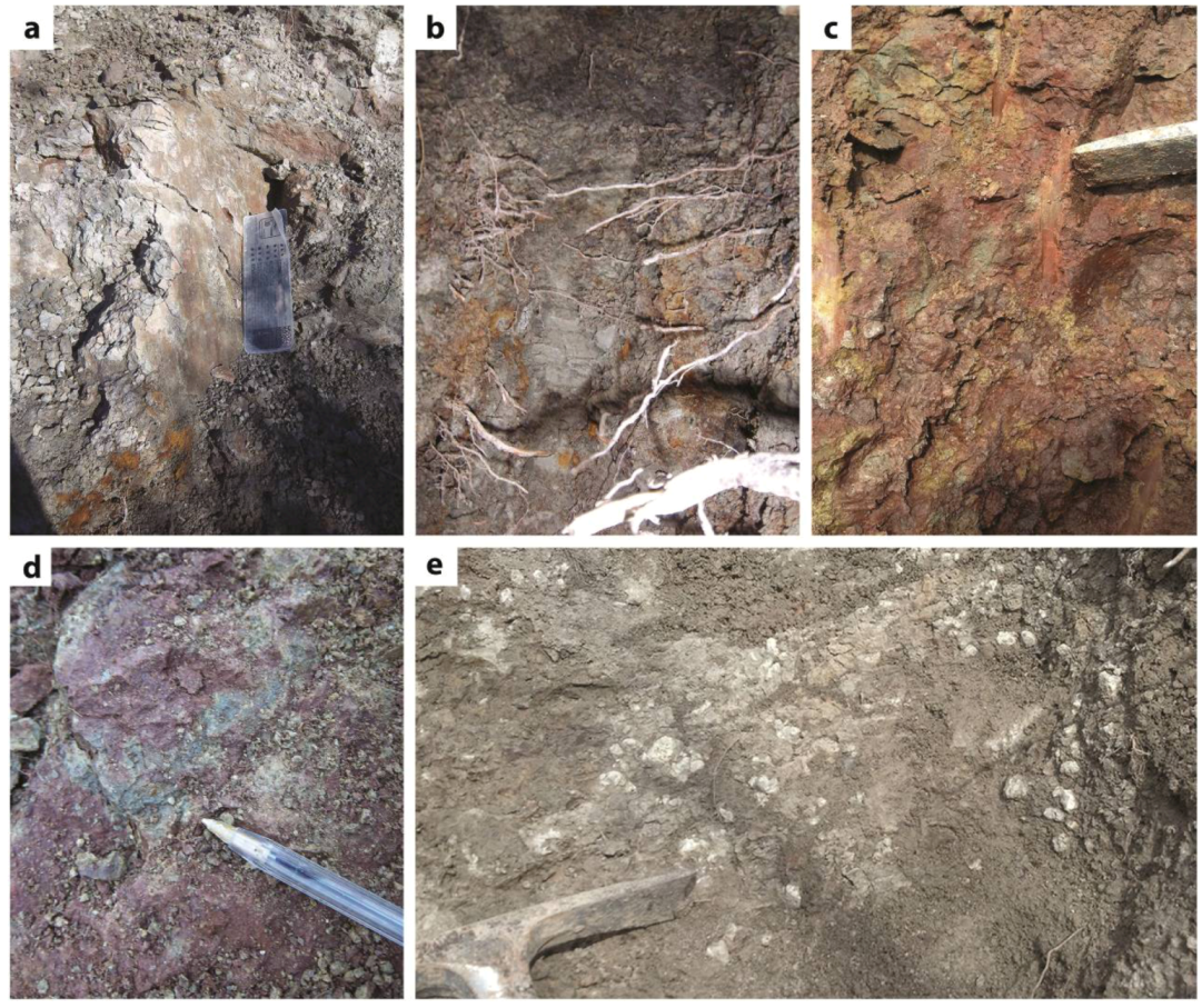
4.1. Description

5. Micromorphology
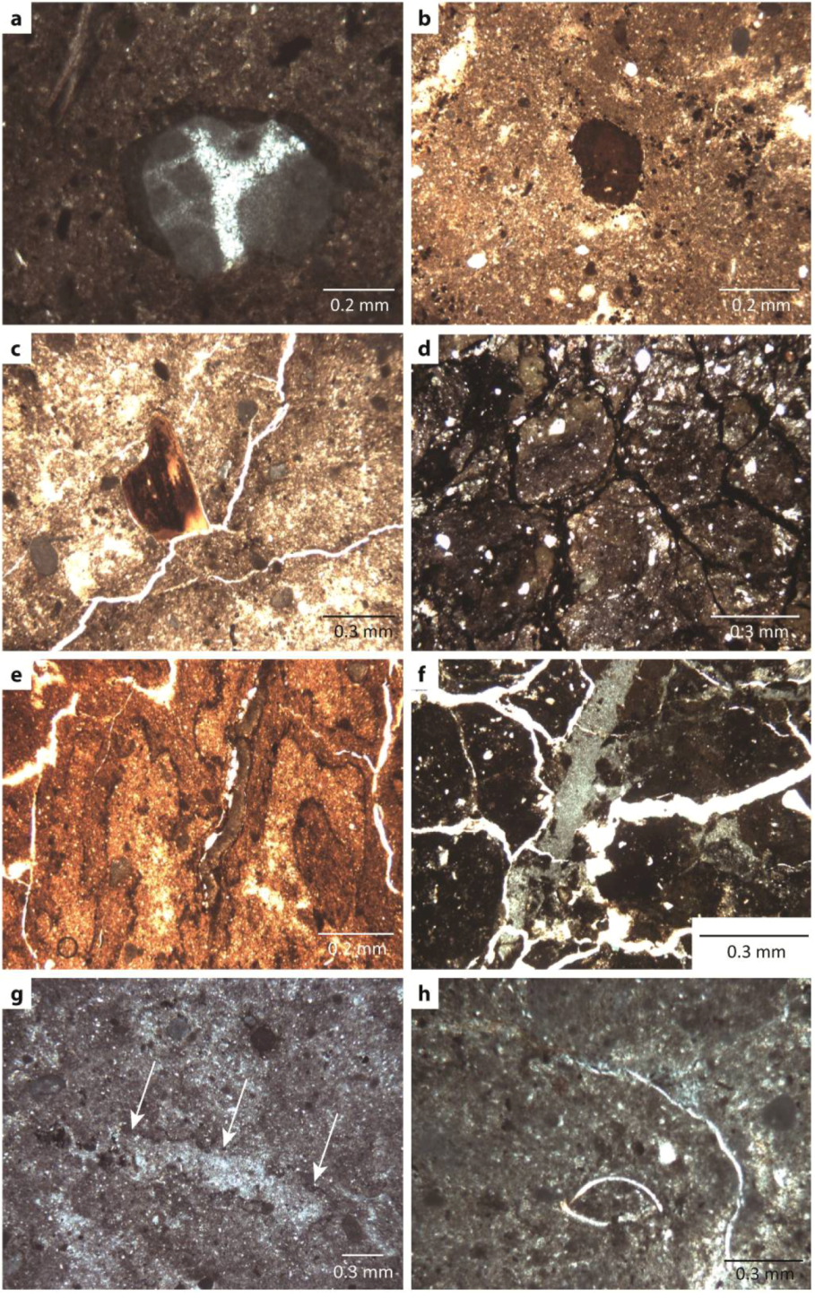
5.1. Description

6. Discussion
6.1. Paleosol Interpretation

6.2. Paleoclimatic Significance
7. Conclusions
Acknowledgments
References
- Cecil, C.B.; Stanton, R.W.; Neuzil, S.G.; Dulong, F.T.; Ruppert, L.F.; Pierce, B.S. Paleoclimate controls on Late Paleozoic sedimentation and peat formation in the central Appalachian basin. Int. J. Coal Geol. 1985, 5, 195–230. [Google Scholar] [CrossRef]
- Joeckel, R.M. Paleosols below the Ames marine unit (Upper Pennsylvanian, Conemaugh Group) in the Appalachian basin, U.S.A.: Variability on an ancient depositional landscape. J. Sediment. Res. 1995, 65, 393–407. [Google Scholar]
- DiMichele, W.A.; Pfefferkorn, H.W.; Gastaldo, R.A. Response of Late Carboniferous and Early Permian plant communities to climate change. Annu. Rev. Earth Planet. Sci. 2001, 29, 461–487. [Google Scholar] [CrossRef]
- DiMichele, W.A.; Cecil, C.B.; Montañez, I.P.; Falcon-Lang, H.J. Cyclic changes in Pennsylvanian paleoclimate and effects on floristic dynamics in tropical Pangaea. Int. J. Coal Geol. 2010, 83, 329–344. [Google Scholar] [CrossRef]
- Hembree, D.I.; Nadon, G.C. A paleopedologic and ichnologic perspective of the terrestrial Pennsylvanian landscape in the distal Appalachian Basin, U.S.A. Palaeogeog. Palaeoclimatol. Palaeoecol. 2011, 312, 138–166. [Google Scholar] [CrossRef]
- Sheldon, N.D.; Tabor, N.J. Quantitative paleoenvironmental and paleoclimatic reconstructions using paleosols. Earth-Sci. Rev. 2009, 95, 1–52. [Google Scholar]
- Hasiotis, S.T. Continental ichnology: Fundamental processes and controls on trace fossil distribution. In Trace Fossils: Concepts, Problems, Prospects; Miller, W., III, Ed.; Elsevier: Amsterdam, The Netherlands, 2007; pp. 268–284. [Google Scholar]
- Kraus, M.J.; Hasiotis, S.T. Significance of different modes of rhizoliths preservation to interpreting paleoenvironmental and paleohydrologic settings: Examples from Paleogene paleosols, Bighorn Basin, Wyoming, U.S.A. J. Sediment. Res. 2006, 76, 633–646. [Google Scholar] [CrossRef]
- Retallack, G.J. Soils of the Past, 2nd ed; Blackwell Science: Oxford, UK, 2001. [Google Scholar]
- Schaetzl, R.; Anderson, S. Soils: Genesis and Geomorphology; Cambridge University Press: Cambridge, UK, 2009. [Google Scholar]
- Kraus, M.J. Paleosols in clastic sedimentary rocks: Their geologic applications. Earth-Sci. Rev. 1999, 47, 41–70. [Google Scholar]
- Greb, S.F.; Pashin, J.C.; Martino, R.L.; Eble, C.F.; Frank, T.D. Appalachian sedimentary cycles during the Pennsylvanian: Changing influences of sea level, climate, and tectonics. Geol. Soc. Am. Spec. Pap. 2008, 441, 235–248. [Google Scholar]
- Scotese, C.R. Carboniferous paleocontinental reconstructions. In Predictive Stratigraphic Analysis—Concept and Application; Cecil, C.B., Edgar, N.T., Eds.; U.S. Government Printing Office: Washington, DC, USA, 1994; pp. 3–6. [Google Scholar]
- Heckel, P.H. Glacial-eustatic base-level—Climatic model for Late Middle to Late Pennsylvanian coal-bed formation in the Appalachian Basin. J. Sediment. Res. 1995, 65B, 348–356. [Google Scholar]
- Lebold, J.G.; Kammer, T.W. Gradient analysis of faunal distributions associated with rapid transgression and low accommodation space in a Late Pennsylvanian marine embayment: Biofacies of the Ames Member (Glenshaw Formation, Conemaugh Group) in the northern Appalachian Basin, USA. Palaeogeog. Palaeoclimatol. Palaeoecol. 2006, 231, 291–314. [Google Scholar] [CrossRef]
- Busch, R.M.; Rollins, H.B. Correlation of Carboniferous strata using a hierarchy of transgressive-regressive units. Geology 1984, 12, 471–474. [Google Scholar] [CrossRef]
- Ross, C.A.; Ross, J.R. Late Paleozoic sea levels and depositional sequences. In Timing and Depositional History of Eustatic Sequences: Constraints on Seismic Stratigraphy; Ross, C.A., Haman, D., Eds.; Cushman Foundation for Foraminiferal Research: Washington, DC, USA, 1987; pp. 137–149, Special Publication No. 24. [Google Scholar]
- Heckel, P.H. Evaluation of evidence for glacio-eustatic control over marine Pennsylvanian cyclothems in North America and consideration of possible tectonic effects. SEPM Concepts Sedimentol. Paleontolog. 1994, 4, 65–87. [Google Scholar]
- Cecil, C.B.; Dulong, F.T.; West, R.R.; Stamm, R.; Wardlaw, B.; Edgar, N.T. Climate controls on the stratigraphy of a Middle Pennsylvanian cyclothem in North America. SEPM Spec. Publ. 2003, 77, 151–182. [Google Scholar]
- Nadon, G.C.; Kelly, R.R. The constraints of glacial eustasy and low accommodation on sequence-stratigraphic interpretations of Pennsylvanian strata, Conemaugh Group, Appalachian basin, U.S.A. Am. Assoc. Pet. Geol. Stud. Geol. 2004, 51, 29–44. [Google Scholar]
- Donaldson, A.C.; Renton, J.J.; Presley, M.W. Pennsylvanian deposystems and paleoclimates of the Appalachians. Int. J. Coal Geol. 1985, 5, 167–193. [Google Scholar] [CrossRef]
- Sturgeon, M.T. The Geology and Mineral Resources of Athens County, Ohio; Ohio Division of Geological Survey: Columbus, OH, USA, 1958. [Google Scholar]
- Martino, R.L. Sequence stratigraphy of the Glenshaw Formation (Middle–Late Pennsylvanian) in the central Appalachian basin. Am. Assoc. Pet. Geol. Stud. Geol. 2004, 51, 1–28. [Google Scholar]
- Condit, D.D. The Conemaugh Formation in Southern Ohio. Ohio Nat. 1909, 9, 482–488. [Google Scholar]
- Munsell Color, Munsell Rock Color Charts; Munsell Color: Baltimore, MD, USA, 2001.
- Mack, G.H.; James, W.C.; Monger, H.C. Classification of paleosols. Geol. Soc. Am. Bull. 1993, 105, 129–136. [Google Scholar]
- NRCS Soils. In Keys to Soil Taxonomy, 11th ed; USDA Natural Resources Conservation Service: Washington, DC, USA, 2010.
- Brewer, R. Fabric and Mineral Analysis of Soils, 2nd ed; Krieger: New York, NY, USA, 1976. [Google Scholar]
- Wilding, L.P.; Tessier, D. Genesis of Vertisols: Shrink-swell phenomena. In Vertisols: Their Distribution, Properties, Classification, and Management; Wilding, L.P., Puentes, R., Eds.; Texas A&M University Printing Center: College Station, TX, USA, 1988; pp. 55–81. [Google Scholar]
- Coulombe, C.E.; Wilding, L.P.; Dixon, J.B. Overview of Vertisols: Characteristics and impacts on society. Adv. Agron. 1996, 57, 289–375. [Google Scholar]
- Jayawardane, N.S.; Greacen, E.L. The nature of swelling in soils. Austral. J. Soil Res. 1987, 25, 107–113. [Google Scholar] [CrossRef]
- Tabor, N.J.; Montañez, I.P.; Scotese, C.R.; Poulsen, C.J.; Mack, G.H. Paleosol archives of environmental and climatic history in paleotropical western Pangea during the latest Pennsylvanian through Early Permian. In Resolving the Late Paleozoic Ice Age in Time and Space; Frank, T.D., Isbell, J.L., Eds.; Geological Society of America: Boulder, CO, USA, 2008; pp. 291–304. [Google Scholar]
- Bromley, R.G. Trace Fossils: Biology, Taphonomy and Applications, 2nd ed; Chapman & Hall: London, UK, 1996. [Google Scholar]
- Gile, L.H.; Peterson, F.F.; Grossman, R.B. Morphological and genetic sequences of carbonate accumulation in desert soils. Soil Sci. 1966, 101, 347–360. [Google Scholar]
- Salomons, W.; Goudie, A.; Mook, W.G. Isotopic composition of calcrete deposits from Europe, Africa, and India. Earth Surf. Proc. Landf. 1978, 3, 43–57. [Google Scholar]
- Treadwell-Steitz, C.; McFadden, L.D. Influence of parent material and grain size on carbonate coatings in gravelly soils, Palo Duro Wash, New Mexico. Geoderma 2000, 94, 1–22. [Google Scholar] [CrossRef]
- Stiles, C.A.; Mora, C.I.; Driese, S.G.; Robinson, A.C. Distinguishing climate and time in the soil record: Mass-balance trends in Vertisols from the Texas coastal prairie. Geology 2003, 31, 331–334. [Google Scholar] [CrossRef]
- Kraus, M.J. Lower Eocene alluvial paleosols: Pedogenic development, stratigraphic relationships, and paleosol/landscape associations. Palaeogeog. Palaeoclimatol. Palaeoecol. 1997, 129, 387–406. [Google Scholar] [CrossRef]
- Birkeland, P.W. Soils and Geomorphology; Oxford University Press: New York, NY, USA, 1999. [Google Scholar]
- Jenny, H. Factors of Soil Formation; McGraw-Hill: New York, NY, USA, 1941. [Google Scholar]
- Mack, G.H.; James, W.C. Paleoclimate and the global distribution of paleosols. J. Geol. 1994, 102, 360–366. [Google Scholar]
- Royer, D.L. Depth to pedogenic carbonate horizon as a paleoprecipitation indicator. Geology 1999, 27, 1123–1126. [Google Scholar] [CrossRef]
- Driese, S.G.; Ober, E.G. Paleopedologic and paleohydrologic records of precipitation seasonality from Early Pennsylvanian “underclay” paleosols, USA. J. Sediment. Res. 2005, 75, 997–1010. [Google Scholar] [CrossRef]
© 2012 by the authors; licensee MDPI, Basel, Switzerland. This article is an open-access article distributed under the terms and conditions of the Creative Commons Attribution license (http://creativecommons.org/licenses/by/3.0/).
Share and Cite
Dzenowski, N.D.; Hembree, D.I. Examining Local Climate Variability in the Late Pennsylvanian Through Paleosols: An Example from the Lower Conemaugh Group of Southeastern Ohio, USA. Geosciences 2012, 2, 260-276. https://doi.org/10.3390/geosciences2040260
Dzenowski ND, Hembree DI. Examining Local Climate Variability in the Late Pennsylvanian Through Paleosols: An Example from the Lower Conemaugh Group of Southeastern Ohio, USA. Geosciences. 2012; 2(4):260-276. https://doi.org/10.3390/geosciences2040260
Chicago/Turabian StyleDzenowski, Nicole D., and Daniel I. Hembree. 2012. "Examining Local Climate Variability in the Late Pennsylvanian Through Paleosols: An Example from the Lower Conemaugh Group of Southeastern Ohio, USA" Geosciences 2, no. 4: 260-276. https://doi.org/10.3390/geosciences2040260