Article

Identifying Spatio-Temporal Landslide Hotspots on North Island, New Zealand, by Analyzing Historical and Recent Aerial Photography

1
Department of Geoinformatics–Z_GIS, University of Salzburg, Schillerstrasse 30, 5020 Salzburg, Austria
2
Landcare Research, Private Bag 11052, Manawatu Mail Centre, Palmerston North 4442, New Zealand
3
Landcare Research, P.O. Box 69040, Lincoln 7640, New Zealand
*
Author to whom correspondence should be addressed.
Geosciences 2016, 6(4), 48; https://doi.org/10.3390/geosciences6040048
Submission received: 30 June 2016 / Revised: 21 October 2016 / Accepted: 27 October 2016 / Published: 2 November 2016
(This article belongs to the Special Issue Mapping and Assessing Natural Disasters Using Geospatial Technologies)

Abstract

:
Accurate mapping of landslides and the reliable identification of areas most affected by landslides are essential for advancing the understanding of landslide erosion processes. Remote sensing data provides a valuable source of information on the spatial distribution and location of landslides. In this paper we present an approach for identifying landslide-prone “hotspots” and their spatio-temporal variability by analyzing historical and recent aerial photography from five different dates, ranging from 1944 to 2011, for a study site near the town of Pahiatua, southeastern North Island, New Zealand. Landslide hotspots are identified from the distribution of semi-automatically detected landslides using object-based image analysis (OBIA), and compared to hotspots derived from manually mapped landslides. When comparing the overlapping areas of the semi-automatically and manually mapped landslides the accuracy values of the OBIA results range between 46% and 61% for the producer’s accuracy and between 44% and 77% for the user’s accuracy. When evaluating whether a manually digitized landslide polygon is only intersected to some extent by any semi-automatically mapped landslide, we observe that for the natural-color images the landslide detection rate is 83% for 2011 and 93% for 2005; for the panchromatic images the values are slightly lower (67% for 1997, 74% for 1979, and 72% for 1944). A comparison of the derived landslide hotspot maps shows that the distribution of the manually identified landslides and those mapped with OBIA is very similar for all periods; though the results also reveal that mapping landslide tails generally requires visual interpretation. Information on the spatio-temporal evolution of landslide hotspots can be useful for the development of location-specific, beneficial intervention measures and for assessing landscape dynamics.

Graphical Abstract

1. Introduction

Landslide erosion is a serious land management problem in many parts of the world, and especially in New Zealand where a combination of steep erodible hill country, a maritime climate featuring frequent and intense rainstorms, and recent forest clearance for pastoral farming have led to extensive landslide erosion on many parts of the country’s hill country farmland. Effective mitigation measures against landslide erosion and its consequences require a detailed understanding of the location, extent, and severity of landsliding. In New Zealand, this usually relies on detailed manual mapping from aerial photography [1] and, more recently, spectral classification of regional satellite imagery following major storm events [2]. For catchment- to farm-scale applications, however, manual image interpretation and mapping has to date been the most-used method for accurately identifying and mapping landsliding, but it is a very slow and tedious process and is thus limited to studies of relatively small areas and can be difficult to implement in practice. In addition, the quality of the resulting landslide maps depends on the experience of the investigator, the purpose of the mapping, the scale, and the data used [3,4,5,6].
Just as the availability and quality of remote sensing data steadily increases, so too do the demands for extracting relevant geospatial information in a semi-automated or even fully automated manner. Optical remote sensing imagery constitutes a valuable and cost-effective source for the development of such classification techniques that offer the potential to significantly improve existing manual landslide mapping approaches, especially when combined with a degree of manual interpretation to create a “hybrid” approach to landslide identification. For example, landslide inventory maps can be prepared using such techniques [7].
The selection of an appropriate technique depends on the purpose of the inventory, the size of the coverage, the time required by investigators, and the available resources [7,8,9,10]. Conventional approaches for landslide recognition comprise resource- and time-consuming ground surveys and visual image interpretation using very high resolution (VHR) satellite or aerial photographs [11,12] based on morphological appearance [13]. High resolution (HR) imagery is used for delineating larger landslides [14]. While visual interpretation is still the most common procedure for landslide mapping, recently, there has been a trend towards semi-automated landslide mapping approaches based on remote sensing data [15]. Efficient image analysis techniques have opened a new era, particularly for studying denied-access, difficult-access, or remote sites [16], but also for performing retrospective analysis based on historical images. Current approaches can basically be split into pixel-based and object-based categories [12,17].
Over the last decade, object-based image analysis (OBIA) has been increasingly used for semi-automated landslide mapping using remote sensing data [6,18,19,20,21,22,23,24]. OBIA, recently recognized as a new paradigm in remote sensing and Geographic Information Science [25], enables researchers to work seamlessly with existing multi-scale geospatial data by combining image processing and GIS functionalities in one interlinked framework [26,27]. OBIA allows the use of spectral, spatial, textural, contextual, and morphological properties. Geomorphological features such as landslides can be treated as aggregates of pixels and can be grouped into homogeneous objects, providing additional information on topological relationships of neighborhood, embeddedness, or shape [28]. Unlike single pixels, image objects are enriched by a range of features/properties stemming from different data sources that can be used during classification. This is especially useful for VHR imagery, where objects of interest are usually significantly larger than the pixel size (H-resolution situation [29]). Optical imagery is most often used in combination with a digital elevation model (DEM) and its derivatives such as slope or curvature. However, relatively few studies in literature so far have used aerial photographs for object-based landslide mapping [24,30,31,32]. Even less research has been done for semi-automatically detecting landslides on panchromatic images, even though the creation of historical landslide inventory maps relies on the analysis of remote sensing data that has been acquired over the past few decades and is most often only available in black and white [23]. A major reason therefore is that the limited spectral information of panchromatic images hampers the differentiation of classes and the detection of features of interest. This is particularly true for semi-automated methods, since they mainly rely on thresholds derived from multispectral bands [23]. However, brightness thresholds from panchromatic images can be used for detecting landslide-affected areas, since these areas tend to appear brighter due to a loss of vegetation and the exposure of fresh rock and bare soil [33].
Manually or semi-automatically mapped landslides from optical images can be used as input for creating landslide hotspot (or density) maps, which are ideal for an easy-to-grasp visual representation of the worst landslide-affected areas after a triggering event (e.g., as produced by the Earthquakes without Frontiers project following the earthquake in Nepal in April 2015 [34]). A few studies investigated the spatial patterns of PSI (Persistent Scatterer Interferometry) point targets for slow moving landslides using synthetic aperture radar (SAR) data complemented by landslide inventories for the identification of landslide hotspots [35,36,37]. Landslide hotspot maps are also valuable when planning field surveys and in situ validation campaigns, so that field work can be prioritized and the time and effort needed significantly reduced [35].
In this study we aim to identify spatio-temporal landslide hotspots by analyzing historical and recent aerial photography for a landslide-prone study site in New Zealand. Landslide hotspots are calculated based on the distribution of semi-automatically detected landslides using OBIA, and compared to hotspots derived from manually mapped landslides.

2. Materials and Methods
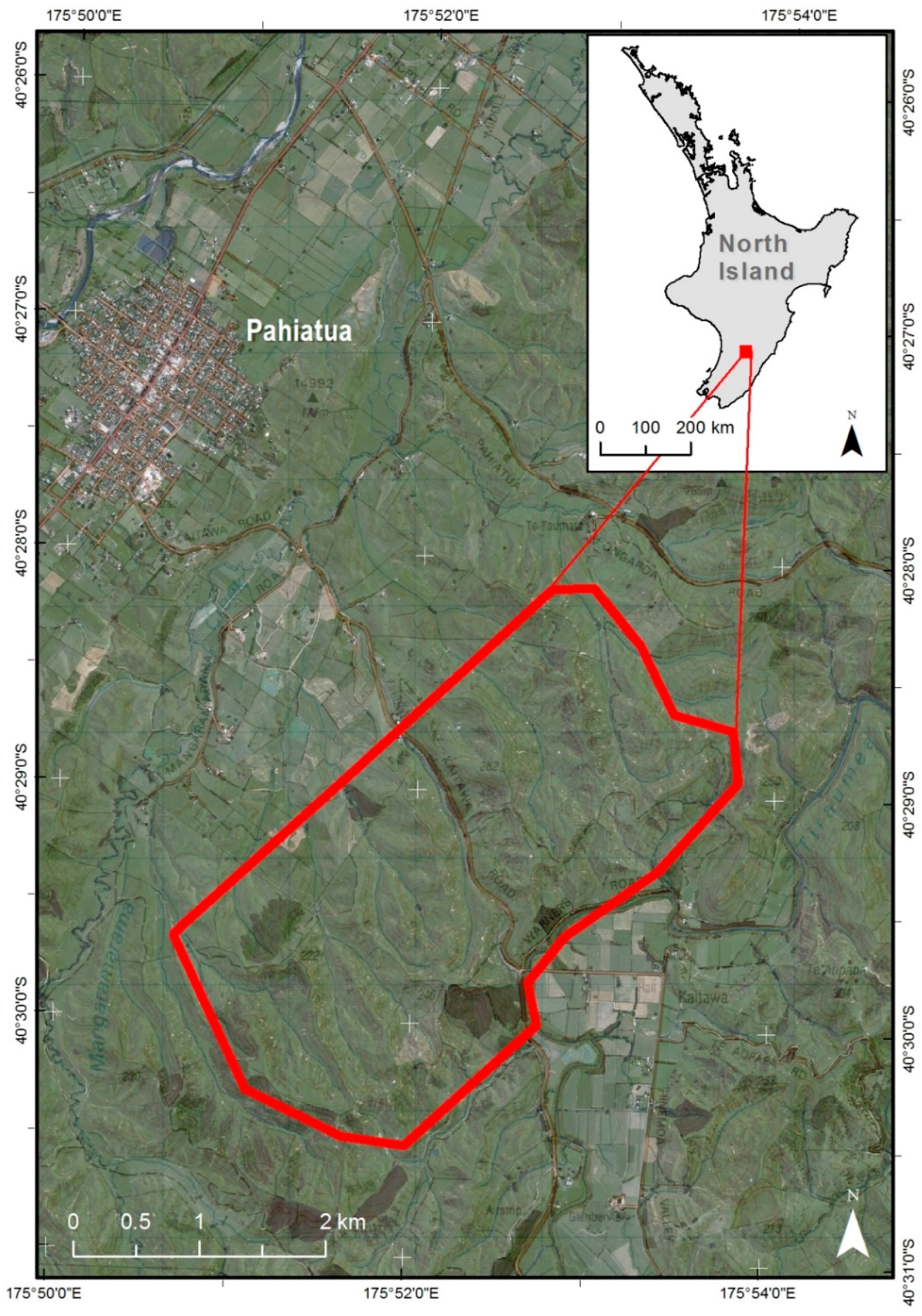
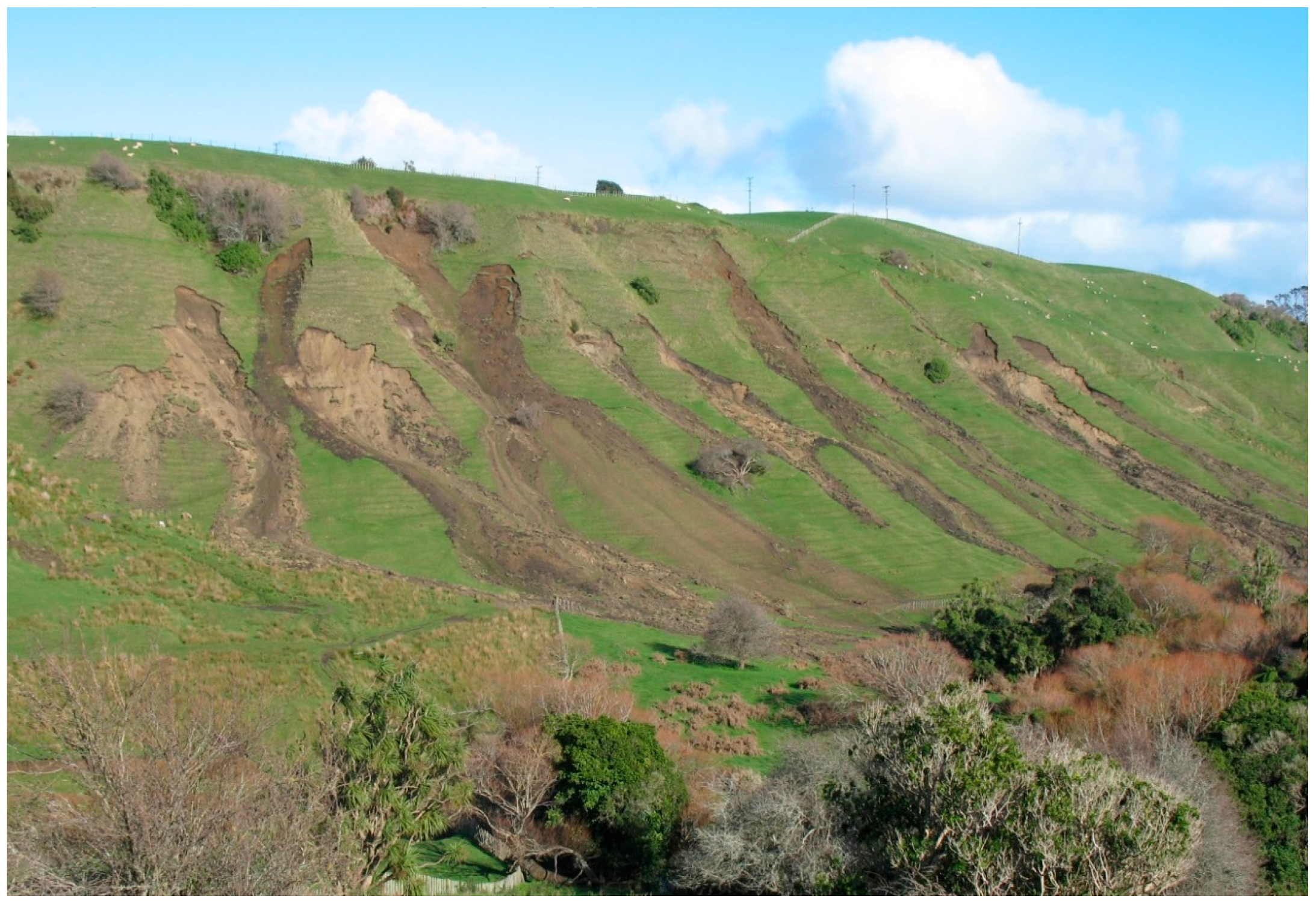
2.1. Study Area

We selected a ~1010 hectare study area located approximately 5 km southeast of the town of Pahiatua, southeastern North Island, New Zealand (Figure 1).
The study site comprises pastoral hill country on moderately indurated Tertiary sandstone and mudstone, with relief in the order of 100–300 m above sea level and slopes typically in the 16–25 degree range. Most of the area’s indigenous forest cover was cleared following European settlement in the late 1800s and early 1900s and, as a consequence, rain-triggered shallow landslide erosion is common (Figure 2).

2.2. Data

Historical and recent aerial photographs were acquired for five dates ranging from 1944 to 2011 (Table 1) and used for the detection of landslides and identification of spatio-temporal landslide hotspots. Aerial photography was supplied as orthorectified digital images with a nominal positional accuracy of 15 m and a spatial resolution of up to 0.4 m. The photographs from the two most recent dates are available as three-band natural color images (RGB); the older photographs only have a panchromatic band. The photographs from 1944 and 1979 were provided as single mosaicked images; for each of the other dates five tiles were mosaicked into one raster dataset to cover the study area. Additionally, a DEM with 15 m resolution, based on 20 m contour lines available from the Land Information New Zealand (LINZ) [38], was used as ancillary data during landslide mapping, particularly the derived slope information.

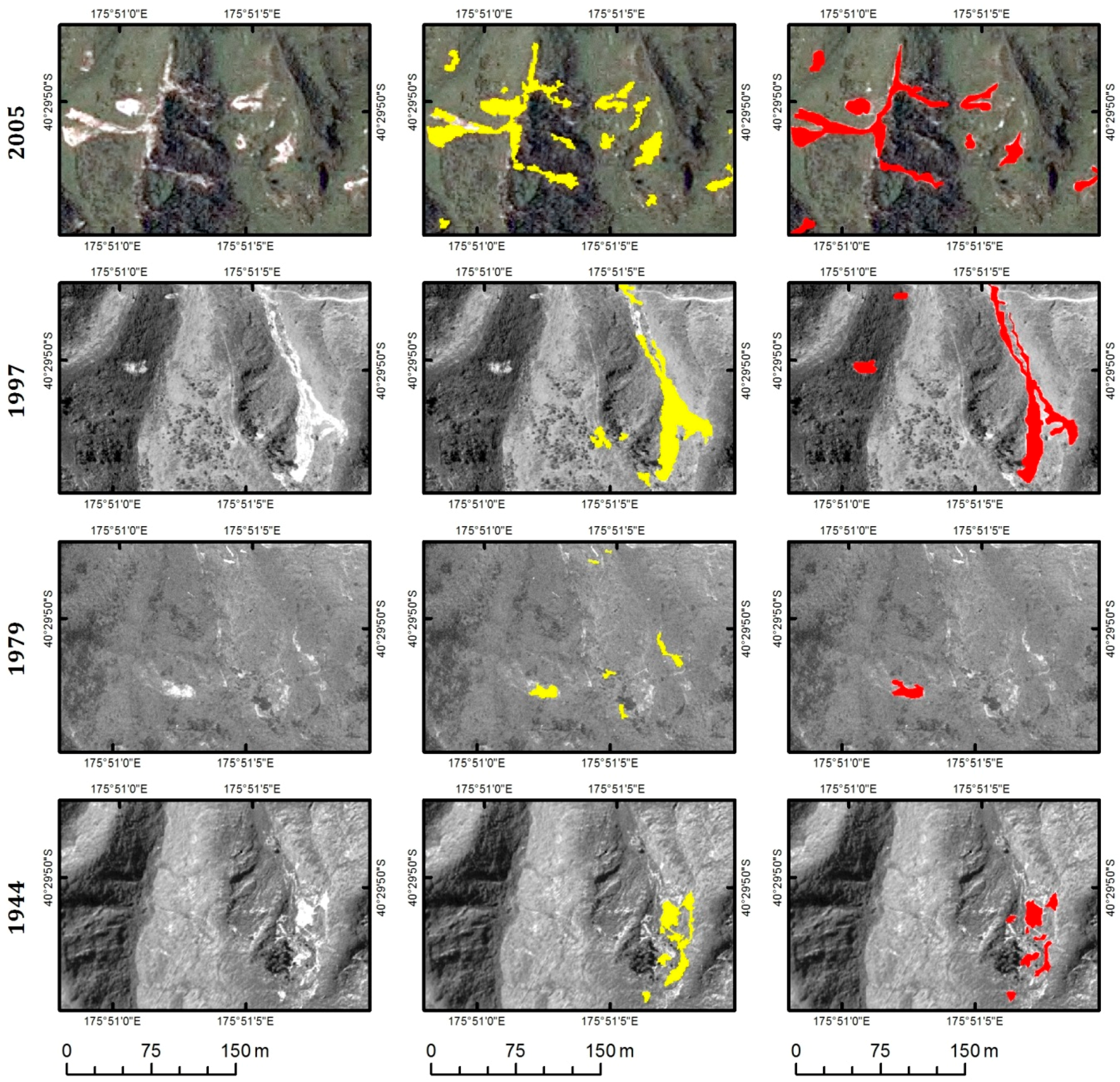
2.3. Visual Landslide Interpretation

Visual landslide interpretation from the orthorectified digital imagery was carried out on-screen using ArcGIS 10.0. Landslides were digitized at scales ranging between 1:600 and 1:1250. Each landslide was then subdivided visually into “scar” and “debris tail” in an effort to separate sediment sources (scars) from areas receiving sediment (debris tails). The aim of the mapping was to identify all landslides that had occurred since the date of the first photography. The mapping results were stored as polygon shapefiles containing delineated landslides, subdivided into scars and debris tails, for each date of photography.

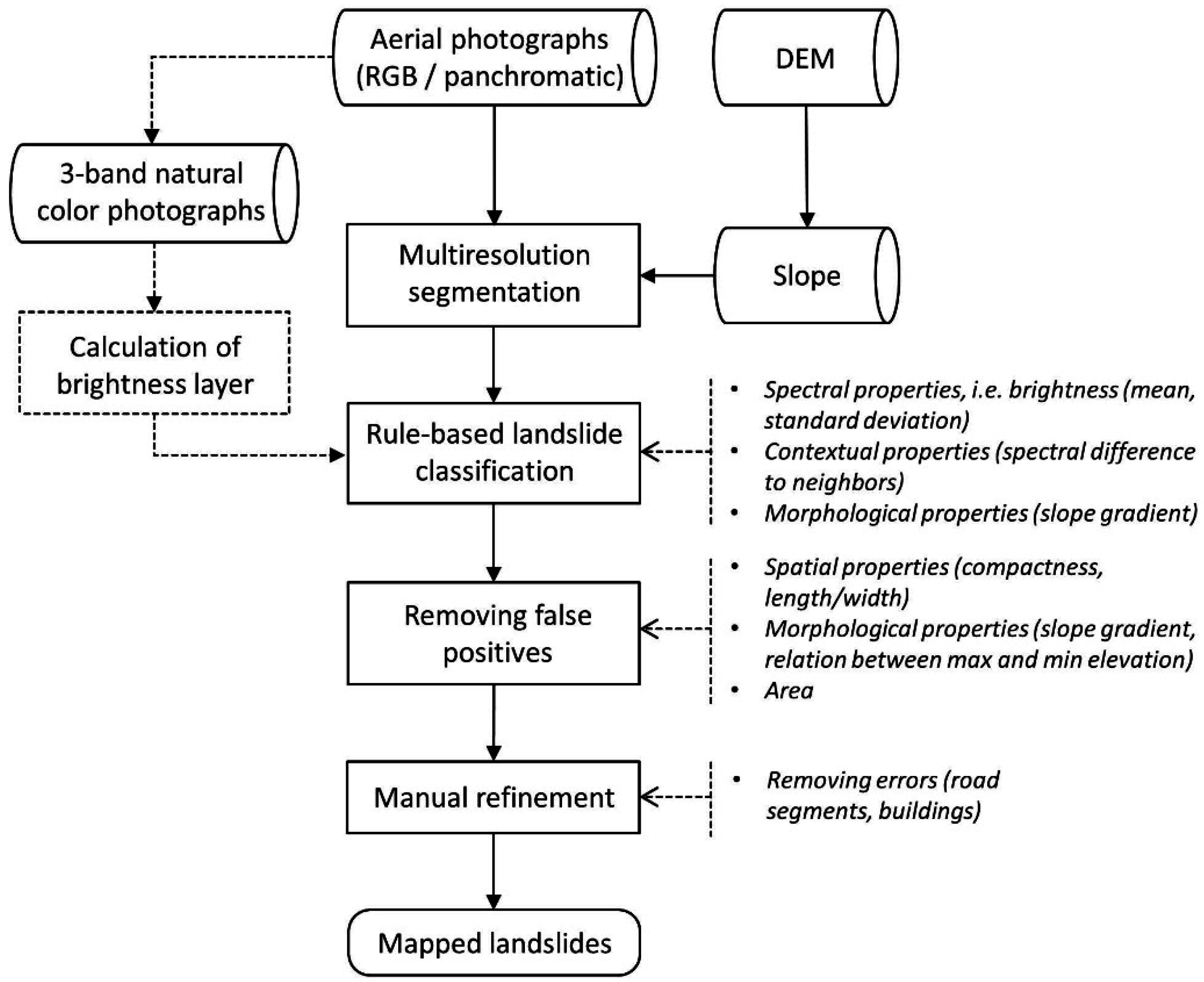
2.4. Semi-Automated Landslide Mapping

For semi-automated landslide mapping, an object-based mapping approach was developed. Analyses were conducted using eCognition (Trimble) software, whereby a set of knowledge-based classification rules were defined. Since aerial photographs from five different points in time were used, major efforts were made to come up with a mapping routine that is applicable to all images. The classification ruleset was developed using the most recent image from 2011 and subsequently transferred to the other aerial photographs. The landslide mapping workflow is shown in Figure 3.
As a first step, the multiresolution segmentation algorithm [39] was applied to create initial image objects that serve as basic units for the classification. Spectral information (panchromatic band or RGB bands, respectively) and the slope layer were considered for image segmentation. Spectral, spatial, morphological, and contextual parameters of image objects were used to classify landslides. However, the spectral values of the RGB bands available for the aerial photographs from 2011 and 2005 were deliberately omitted during rule-based classification. Instead, an average or “panchromatic” brightness layer was calculated for the multispectral images by dividing the sum of the three spectral bands by three. This was done to increase the transferability of the method across the panchromatic images from 1997, 1979, and 1944. For the detection of potential landslide objects, this brightness/panchromatic layer was mostly used, since landslides usually appear brighter than their immediate surroundings on optical images due to the exposure of bare ground [4,33,40]. Next to the mean brightness values of the image objects, the spectral difference between landslide objects and their neighbors was considered. Slope gradient thresholds were always applied in conjunction with other parameters, such as the brightness/panchromatic information, to avoid the classification of image objects with similar spectral characteristics. For example, bright image objects with a mean slope below 5 degrees were excluded from the initial classification of target areas.
To remove false positives from the initial landslide classification, spatial properties of image objects such as compactness (product of the length and the width, divided by the number of pixels) or length/width ratio together with slope gradient thresholds, ranging between <15 and <30 degrees, were used. These parameters were applied since landslide objects appeared to be more compact but at the same time more elongated than false positives. It is hardly possible to define a fixed slope gradient threshold at which a landslide occurs as slope failure has in some cases been observed on gentle slopes of 1–2 degrees [41]. Therefore, next to the varying slope gradients, the relation between the maximum elevation and minimum elevation within an image object also proved to be useful for the elimination of misclassified objects. Finally, after merging the classified landslide objects, very small (<10 m²) or very large polygons (e.g., large quarries) were eliminated. The classified objects were merged to more easily remove some of the remaining false positives afterwards. Apart from the visual interpretation, it was not possible to effectively differentiate between scars and debris tails. Thus, only the landslide-affected area was semi-automatically mapped.
This approach was then transferred to the other aerial photographs, whereby only minor adaptations of thresholds and small changes regarding the usage of specific image properties were necessary. Some remaining errors (e.g., road segments, buildings) were removed manually in a final step, whereby this concerned only the obvious misclassifications and took less than 10 min for each date.

2.5. Identification of Landslide Hotspots

To facilitate a visual comparison of the manually mapped landslides and the landslides mapped with OBIA, hotspot maps were created. The landslide features were rasterized at 1 m cell size and aggregated to 25 m pixel resolution by calculating the sum of 1 m landslide pixels per 25 m cell. The resulting map is a landslide cover map which can also be interpreted as a density map, as it displays the proportion of landslide area covering each pixel (625 m2) in percent. A bilinear interpolation is used to create a smoother representation of the results. Hotspot maps have the advantage that areas most affected by landslides can be immediately identified. The maps also provide a more appropriate scale for comparing results as the general distribution of landslides is more pronounced.

3. Results

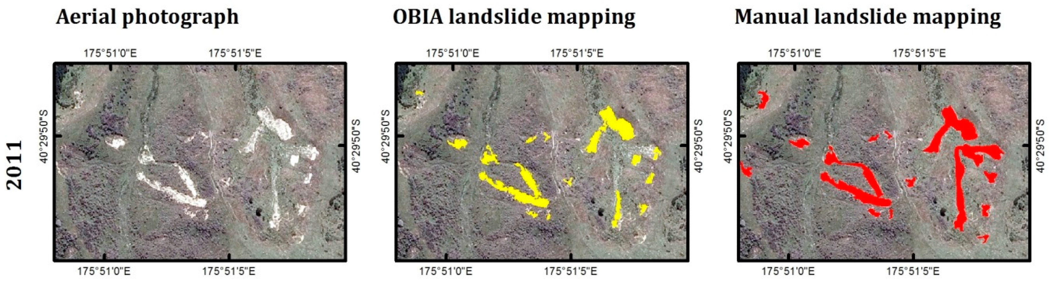
3.1. Landslide Mapping Results

Visual mapping identified a total of 2703 landslide scars and 2343 landslide tails over the five dates of photography mapped. Fewer landslide tails than scars were mapped, as tails had frequently grassed over prior to aerial photography being captured, whereas scars tended to take longer to revegetate owing to a lack of remaining soil on the scar faces. The cumulative area covered by landslide scars was considerably less than that covered by tails, reflecting the fact that sediment generated from even small scars is often spread over a relatively large downslope area.
In contrast to the manual mapping, no differentiation between scars and tails was done during semi-automated mapping. Furthermore, due to the variability of landslides appearance it was hardly possible to delineate single landslides as single objects semi-automatically and thus to identify the number of mapped landslides (see also the Discussion section). For both approaches, most landslides were detected based on the data from 2005, since the imagery were taken after a large storm event that triggered a lot of landslides. Figure 4 shows the semi-automated and the manual mapping results for 2005. A subset with the mapping results from each date of the aerial photography is shown in Figure 5.

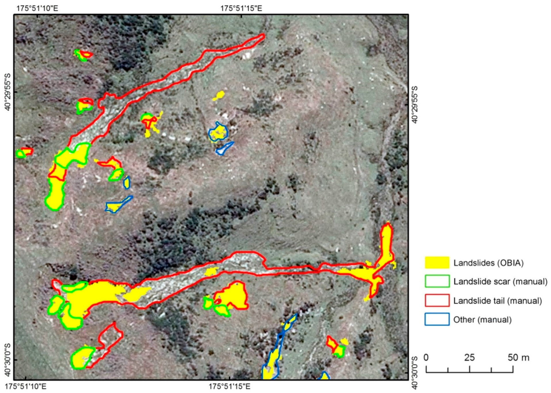
Comparison of Semi-Automated Mapping with Visual Interpretation

For assessing the classification accuracy, the semi-automated OBIA results have been compared to the respective results from visual landslide interpretation, which were used as reference data. To do so, the amount of overlapping area was calculated. Based on this overlapping area the respective producer’s and user’s accuracies were computed [42] (Table 2). The producer’s accuracy was calculated by dividing the correctly classified landslides area (overlap area) by the total area of manually mapped landslides (i.e., the reference data). The user’s accuracy was computed by dividing the correctly classified landslides area (overlap area) by the total landslide area mapped by OBIA.
The (at first glance) moderate accuracy values can be explained by several reasons. The semi-automated detection of landslides with OBIA relies mainly on spectral differences of the landslide body to the surrounding areas (i.e., landslides appear brighter on the aerial photographs). This works well for the landslide source areas, but with limited accuracy for landslide tails, considering the fact that data with limited spectral information was available and only the brightness was used (neither other spectral values nor spectral indices were used). A number of landslide tails were identified during visual interpretation that require a trained eye for detection—a capability that can hardly be directly transferred into computer-based classification rules. Figure 6 shows an example where landslides’ source areas were well detected by the object-based approach, but where several landslide tails were missed due to a lack of distinct spectral, spatial, or morphological characteristics. This also becomes evident when comparing the overall mapped area between the OBIA classification and the manual mapping (Table 2). Apart from the result for 1997, the total area of landslides mapped was less with OBIA. The difference of total area mapped can be explained by the large landslide tails (Figure 6), which were more difficult to identify. The small landslides were more reliably automatically detected with OBIA.
Usually, manual mapping results produced by local experts are often the only reference available, but they cannot constitute a completely true reference as their generation depends on various factors [6]. This should be considered when interpreting the accuracy values.
When not comparing the overlapping area, but rather evaluating whether a manually digitized landslide polygon is only intersected to some extent by any semi-automatically mapped landslide, we observe that for the two natural-color images the landslide detection rate is 83% for 2011 and 93% for 2005; for the panchromatic images the values are slightly lower (67% for 1997, 74% for 1979, and 72% for 1944). Consequently, it can be stated that a large percentage of landslides have been correctly detected by OBIA, but the actual delineation of the landslides varies between the two methods.

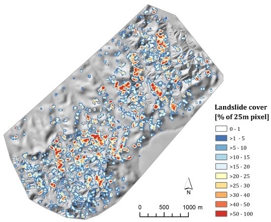
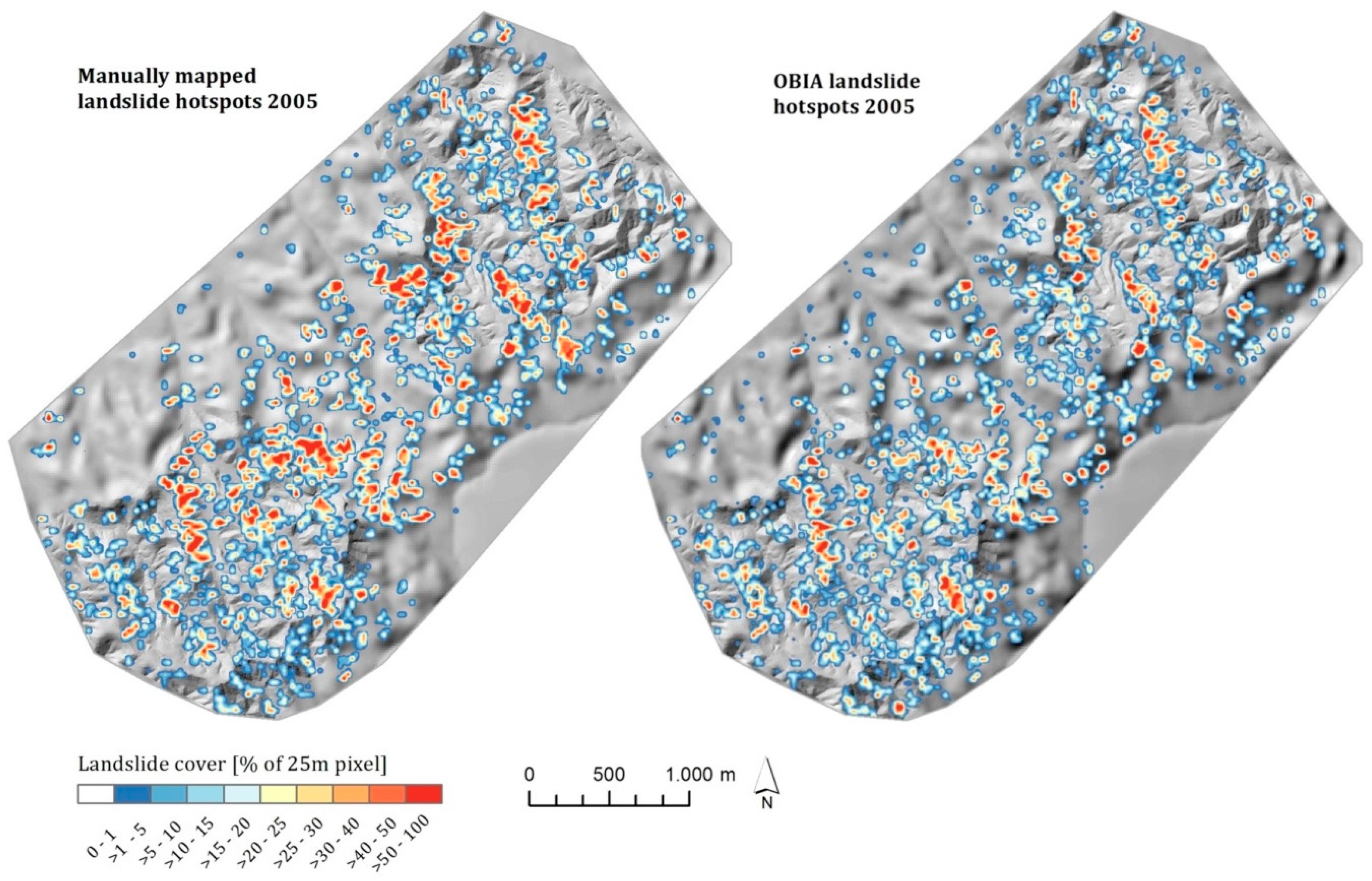
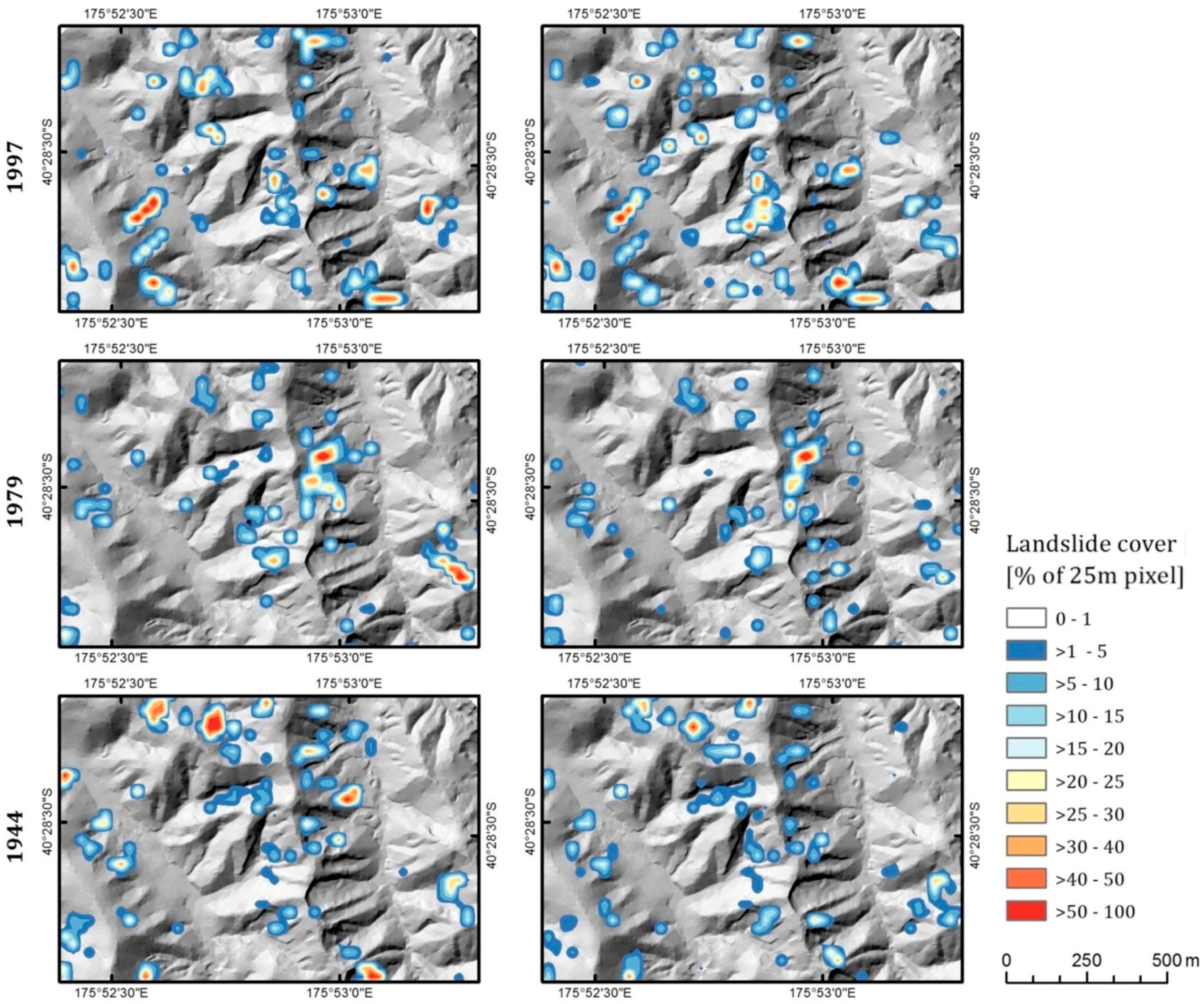
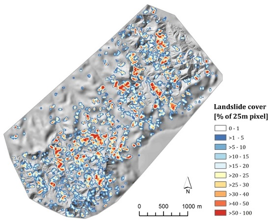
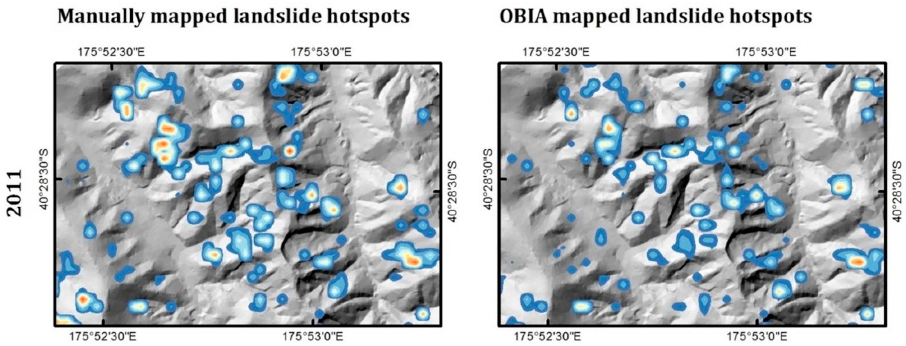
3.2. Landslide Hotspots

A comparison of the landslide hotspot maps (Figure 7 and Figure 8) shows that the distribution of the manually identified landslides and those mapped with OBIA is very similar for all periods. The major difference, which is particularly well observed in the hotpots maps of 2005 (Figure 7), is the proportion that landslides cover an affected area. As stated above, one explanation is the fact that the total area of landslides identified using manual mapping techniques is greater than that detected by OBIA since the detection of landslide tails is a challenging task with a semi-automated approach. A closer inspection of the 2005 results not only shows this to be true, but offers an explanation for the difference of total area mapped. Eighty-five percent of the manually mapped landslide area that does not overlap with the OBIA landslides is classified as landslide tails. These non-overlapping segments of landslides are generally located at lower ends of long narrow debris tails where the grass cover is more quickly restored. Though the OBIA landslides in 2005 are fairly evenly distributed over the scar and tail areas (47.8% to 52.2%, respectively), our results show that mapping lower ends of landslide tails generally requires visual interpretation. However, the hotspot maps confirm that the two different methods of landslide detection render consistently comparable results and that OBIA can be employed to gain rapid insights into the distribution and intensity landslide-affected areas.

4. Discussion

Visual interpretation enables landslide scars and debris tails to be differentiated. It is worth noting that fewer landslide tails than scars were mapped, because tails had frequently grassed over prior to aerial photography being captured, whereas scars tend to take longer to revegetate owing to a lack of remaining soil on the scar faces. On the other hand, the cumulative area covered by landslide scars was considerably less than that covered by tails, reflecting the fact that sediment generated from even small scars is often spread over a relatively large downslope area.
Such a differentiation of landslide scars and debris tails could not be done with OBIA, because the debris tails did not show distinct spectral characteristics that would have facilitated their reliable detection. Semi-automated (OBIA) mapping results would be sensitive to the length of time elapsed between a landslide triggering event and the next available image (Table 3). Imagery taken immediately after a heavy rainfall is ideal for capturing the full extent of landslides, and is a significant reason for the large area of landslides mapped in 2005 following the storm event in 2004. In contrast, no large rainfall event precedes the 2011 photography, which may indicate that old landslide scars from the 2004 event have been captured. An accurate differentiation of the actual source areas (scars) and deposition areas (tails) by OBIA may be facilitated with additional imagery taken a number of weeks after an event when the depositional tails will have started to revegetate, whilst the scars would still be clearly visible.
The manual mapping approach shows advantages over the semi-automated method for delineating single landslides or splitting up compound landslide complexes into separate landslides [43]. Since segmentation-derived image objects rarely correspond to single landslides due to over- or undersegmentation and the variability inherent to landslides, the exact demarcation of objects that represent single landslides is a major challenge and further research is needed in this direction. Advanced algorithms for object boundary refinement (e.g., split and merge based on specific conditions) could be used to improve the delineation of single landslides. However, the creation of “meaningful” objects with regard to a particular context or aim can be very complex [25]. Thus, only landslide-affected areas and not the number of landslides were mapped by OBIA.
Guzzetti et al. [7] review conventional methods for the production of landslide inventory maps and examine the role of new techniques based on modern technologies. The review discusses the value and limitations of geomorphological field mapping and the interpretation of stereoscopic aerial photographs and evaluates semi-automatic approaches for the recognition of landslides, including the OBIA method. Guzzetti et al. [7] conclude that the systematic use of semi-automatic techniques limits subjectivity and can contribute to improving the reproducibility of landslide maps.
Manual mapping, while generally more accurate than semi-automated methods, is also a very time-consuming process, and any large-scale mapping task would presumably benefit from a degree of automation [30]. A hybrid approach that combines both semi-automated feature delineation and manual interpretation could improve the whole mapping process and can lead to acceptably accurate mapping results with the potential to greatly reduce the time and effort needed for generating landslide inventories. For example, the initial delineation of areas of bare ground (i.e., the rapid identification of target areas) could be automated, followed by a manual refinement by an experienced interpreter.
The produced landslide hotspot maps show that the distribution of the manually identified landslides and those mapped with OBIA is very similar for all periods. Hotspot maps have the advantage that areas most affected by landslides can be immediately identified, even if the accuracy of the actually mapped landslides is limited. Hotspots maps created on the basis of OBIA mapping results can be produced very quickly and thus might be particularly valuable for the rapid information provision after landslide triggering events.

5. Conclusions

Findings from the analysis of recent and historical images can provide useful information for predicting unstable areas prone to erosion and landslides, and thus can serve as input for spatial planning, risk zone identification, and hazard mitigation. Therefore, improving our capability to map landslides and to identify spatio-temporal landslide hotspots has considerable practical implications and socio-economic importance. While landslide erosion is already a problem in many areas under present-day climate regimes, future climate change is likely to cause significant environmental changes which may lead to even more frequent landslide triggering events (heavy rainstorms). With this in mind, the significance of (semi)-automated and reliable methods that are widely applicable for monitoring landscape changes becomes evident.

Acknowledgments

This research has been partly supported by the Austrian Research Promotion Agency FFG in the Austrian Space Applications Program (ASAP 11) through the project “Land@Slide” (contract no: 847970). We would like to thank Graeme Vial and Peter Hewitt who kindly allowed us to access their Pahiatua properties to carry out field work. New Zealand Aerial Mapping Limited, Aerial Surveys Ltd. and Horizons Regional Council (Manawatu, New Zealand) are thanked for supplying us with aerial imagery. The New Zealand mapping was funded in part by a subcontract from AgResearch as part of the Clean Water Productive Land Research programme funded by the New Zealand Ministry of Business, Innovation and Employment contract C10X1006.

Author Contributions

Daniel Hölbling did the object-based landslide mapping and the accuracy assessment. Harley Betts performed the visual landslide interpretation, DEM analyses, and the pre-processing of the aerial photographs. Raphael Spiekermann was responsible for the landslide hotspot analysis. Daniel Hölbling, Harley Betts, and Raphael Spiekermann wrote the different sections of the paper. Chris Philips provided valuable background information and revised the manuscript.

Conflicts of Interest

The authors declare no conflict of interest. The founding sponsors had no role in the design of the study; in the collection, analyses, or interpretation of data; in the writing of the manuscript, and in the decision to publish the results.

Abbreviations

The following abbreviations are used in this manuscript:
DEMDigital Elevation Model
HRHigh Resolution
LINZLand Information New Zealand
OBIAObject-based Image Analysis
PSIPersistent Scatterer Interferometry
RGBRed, Green, Blue
SARSynthetic Aperture Radar
VHRVery High Resolution

References

  1. De Rose, R.C.; Trustrum, N.A.; Blaschke, P.M. Post-deforestation soil loss from steepland hillslopes in Taranaki, New Zealand. Earth Surf. Proc. Land 1996, 18, 131–144. [Google Scholar] [CrossRef]
  2. Dymond, J.R.; Ausseil, A.-G.; Shepherd, J.D.; Buettner, L. Validation of a region-wide model of landslide susceptibility in the Manawatu-Wanganui region of New Zealand. Geomorphology 2006, 74, 70–79. [Google Scholar] [CrossRef]
  3. Basher, L.R.; Betts, H.D.; De Rose, R.C.; Lynn, I.H.; Marden, M.; McNeill, S.J.; Sutherland, A.; Willoughby, J.; Page, M.J.; Rosser, B. Accounting for the Effects of Mass-movement Erosion on Soil Carbon Stocks in the Soil Carbon Monitoring System: A Pilot Project, Landcare. Research Contract Report LC 288; Landcare Research: Lincoln, New Zealand, 2011; p. 89. [Google Scholar]
  4. De Rose, R.C. Slope control on the frequency distribution of shallow landslides and associated soil properties, North Island, New Zealand. Earth Surf. Proc. Land 2013, 38, 356–371. [Google Scholar] [CrossRef]
  5. Galli, M.; Ardizzone, F.; Cardinali, M.; Guzzetti, F.; Reichenbach, P. Comparing landslide inventory maps. Geomorphology 2008, 94, 268–289. [Google Scholar] [CrossRef]
  6. Hölbling, D.; Friedl, B.; Eisank, C. An object-based approach for semi-automated landslide change detection and attribution of changes to landslide classes in northern Taiwan. Earth Sci. Inform. 2015, 8, 327–335. [Google Scholar] [CrossRef]
  7. Guzzetti, F.; Mondini, A.C.; Cardinali, M.; Fiorucci, F.; Santangelo, M.; Chang, K.-T. Landslide inventory maps: New tools for an old problem. Earth-Sci. Rev. 2012, 112, 42–66. [Google Scholar] [CrossRef]
  8. Guzzetti, F.; Cardinali, M.; Reichenbach, P.; Carrara, A. Comparing Landslide Maps: A Case Study in the Upper Tiber River Basin, Central Italy. Environ. Manag. 2000, 25, 247–263. [Google Scholar] [CrossRef]
  9. Mondini, A.C.; Viero, A.; Cavalli, M.; Marchi, L.; Herrera, G.; Guzzetti, F. Comparison of event landslide inventories: The Pogliaschina catchment test case, Italy. Nat. Hazards Earth Syst. Sci. 2014, 14, 1749–1759. [Google Scholar] [CrossRef]
  10. Van Westen, C.J.; Asch, T.W.J.; Soeters, R. Landslide hazard and risk zonation—Why is it still so difficult? Bull. Eng. Geol. Environ. 2005, 65, 167–184. [Google Scholar] [CrossRef]
  11. Mantovani, F.; Soeters, R.; van Westen, C.J. Remote sensing techniques for landslide studies and hazard zonation in Europe. Geomorphology 1996, 15, 213–225. [Google Scholar] [CrossRef]
  12. Van Westen, C.J.; Castellanos, E.; Kuriakose, S.L. Spatial data for landslide susceptibility, hazard, and vulnerability assessment: An overview. Eng. Geol. 2008, 102, 112–131. [Google Scholar] [CrossRef]
  13. Dikau, R.; Brunsden, D.; Schrott, L.; Ibsen, M.L. Landslide Recognition: Identification, Movement and Causes; Wiley & Sons: Chichester, UK, 1996; p. 274. [Google Scholar]
  14. Singhroy, V. Remote sensing of landslides. In Landslide Hazard and Risk; Glade, T., Anderson, M.G., Crozier, M.J., Eds.; Wiley & Sons: West Sussex, UK, 2005; pp. 469–492. [Google Scholar]
  15. Michoud, C.; Abellan, A.; Derron, M.H.; Jaboyedoff, M. SafeLand Deliverable 4.1. Review of Techniques for Landslide Detection, Fast Characterization, Rapid Mapping and Long-Term Monitoring. 2010, p. 401. Available online: https://www.google.at/url?sa=t&rct=j&q=&esrc=s&source=web&cd=3&cad=rja&uact=8&ved=0ahUKEwi9lcr1p_3PAhUMDcAKHXdnCLEQFggkMAI&url=https%3A%2F%2Fwww.geologie.ac.at%2Fuploads%2Ftx_lumophpinclude%2FfileOutput.php%3Fid%3D726&usg=AFQjCNH8h3smmwM-1wRwAYM1HfTRkqDedA&bvm=bv.136811127,d.bGg (accessed on 31 October 2016).
  16. Coblentz, D.; Pabian, F.; Prasad, L. Quantitative Geomorphometrics for Terrain Characterization. Int. J. Geosci. 2014, 5, 247–266. [Google Scholar] [CrossRef]
  17. Moosavi, V.; Talebi, A.; Shirmohammadi, B. Producing a landslide inventory map using pixel-based and object-oriented approaches optimized by Taguchi method. Geomorphology 2014, 204, 646–656. [Google Scholar] [CrossRef]
  18. Heleno, S.; Matias, M.; Pina, P.; Sousa, A.J. Semiautomated object-based classification of rain-induced landslides with VHR multispectral images on Madeira Island. Nat. Hazards Earth Syst. Sci. 2016, 16, 1035–1048. [Google Scholar] [CrossRef]
  19. Hölbling, D.; Füreder, P.; Antolini, F.; Cigna, F.; Casagli, N.; Lang, S. A Semi-Automated Object-Based Approach for Landslide Detection Validated by Persistent Scatterer Interferometry Measures and Landslide Inventories. Remote Sens. 2012, 4, 1310–1336. [Google Scholar] [CrossRef] [Green Version]
  20. Kurtz, C.; Stumpf, A.; Malet, J.-P.; Gançarski, P.; Puissant, A.; Passat, N. Hierarchical extraction of landslides from multiresolution remotely sensed optical images. ISPRS J. Photogramm. 2014, 87, 122–136. [Google Scholar] [CrossRef]
  21. Lahousse, T.; Chang, K.-T.; Lin, Y. Landslide mapping with multiscale object-based image analysis—A case study in the Baichi watershed, Taiwan. Nat. Hazards Earth Syst. Sci. 2011, 11, 2715–2726. [Google Scholar] [CrossRef] [Green Version]
  22. Lu, P.; Stumpf, A.; Kerle, N.; Casagli, N. Object-oriented change detection for landslide rapid mapping. IEEE Geosci. Remote Sens. 2011, 8, 701–705. [Google Scholar] [CrossRef]
  23. Martha, T.R.; Kerle, N.; van Westen, C.J.; Jetten, V.; Vinod Kumar, K. Object-oriented analysis of multi-temporal panchromatic images for creation of historical landslide inventories. ISPRS J. Photogramm. 2012, 67, 105–119. [Google Scholar] [CrossRef]
  24. Stumpf, A.; Kerle, N. Object-oriented mapping of landslides using Random Forests. Remote Sens. Environ. 2011, 115, 2564–2577. [Google Scholar] [CrossRef]
  25. Blaschke, T.; Hay, G.J.; Kelly, M.; Lang, S.; Hofmann, P.; Addink, E.; Queiroz Feitosa, R.; van der Meer, F.; van der Werff, H.; van Coillie, F.; et al. Geographic Object-Based Image Analysis—Towards a new paradigm. ISPRS J. Photogramm. 2014, 87, 180–191. [Google Scholar] [CrossRef] [PubMed]
  26. Chen, G.; Hay, G.J.; Carvalho, L.; Wulder, M.A. Object-based change detection. Int. J. Remote Sens. 2012, 33, 4434–4457. [Google Scholar] [CrossRef]
  27. Blaschke, T. Object based image analysis for remote sensing. ISPRS J. Photogramm. 2010, 65, 2–16. [Google Scholar] [CrossRef]
  28. Drăguţ, L.; Blaschke, T. Automated classification of landform elements using object-based image analysis. Geomorphology 2006, 81, 330–344. [Google Scholar] [CrossRef]
  29. Strahler, A.H.; Woodcock, C.E.; Smith, J.A. On the nature of models in remote sensing. Remote Sens. Environ. 1986, 20, 121–139. [Google Scholar] [CrossRef]
  30. Hölbling, D.; Betts, H.; Spiekermann, R.; Phillips, C. Semi-automated landslide mapping from historical and recent aerial photography. In Proceedings of the 19th Agile 2016 Conference on Geographic Information Science, Helsinki, Finland, 14–17 June 2016; p. 5.
  31. Moine, M.; Puissant, A.; Malet, J.-P. Detection of landslides from aerial and satellite images with a semi-automatic method. Application to the Barcelonnette basin (Alpes-de-Hautes-Provence, France). In Proceedings of the Landslide Processes: From Geomorphological Mapping to Dynamic Modelling, Strasbourg, France, 6–7 February 2009; pp. 63–68.
  32. Rau, J.-Y.; Jhan, J.-P.; Rau, R.-J. Semiautomatic object-oriented landslide recognition scheme from multisensor optical imagery and DEM. IEEE Trans. Geosci. Remote Sens. 2014, 52, 1336–1349. [Google Scholar] [CrossRef]
  33. Blaschke, T.; Feizizadeh, B.; Hölbling, D. Object-Based Image Analysis and Digital Terrain Analysis for Locating Landslides in the Urmia Lake Basin, Iran. IEEE J. Sel. Top. Appl. 2014, 7, 4806–4817. [Google Scholar] [CrossRef]
  34. Earthquakes without Frontiers. Nepal: UPDATED (28 May) Landslide Inventory Following 25 April Nepal Earthquake. Available online: http://ewf.nerc.ac.uk/2015/05/28/nepal-updated-28-may-landslide-inventory-following-25-april-nepal-earthquake (accessed on 5 October 2016).
  35. Bianchini, S.; Cigna, F.; Righini, G.; Proietti, C.; Casagli, N. Landslide hotspot mapping by means of Persistent Scatterer Interferometry. Environ. Earth Sci. 2012, 67, 1155–1172. [Google Scholar] [CrossRef]
  36. Lu, P.; Casagli, N.; Catani, F.; Tofani, V. Persistent Scatterers Interferometry Hotspot and Cluster Analysis (PSI-HCA) for detection of extremely slow-moving landslides. Int. J. Remote Sens. 2012, 33, 466–489. [Google Scholar] [CrossRef]
  37. Lu, P.; Bai, S.; Casagli, N. Investigating Spatial Patterns of Persistent Scatterer Interferometry Point Targets and Landslide Occurrences in the Arno River Basin. Remote Sens. 2014, 6, 6817–6843. [Google Scholar] [CrossRef]
  38. Land Information New Zealand (LINZ). NZ Contours (Topo, 1:50k). Available online: https://data.linz.govt.nz/layer/768-nz-contours-topo-150k (accessed on 5 October 2016).
  39. Baatz, M.; Schäpe, A. Multiresolution Segmentation—An optimization approach for high quality multi-scale image segmentation. In Angewandte Geographische Informationsverarbeitung XII; Strobl, J., Blaschke, T., Griesebner, G., Eds.; Wichmann: Heidelberg, Germany, 2000; pp. 12–23. [Google Scholar]
  40. Behling, R.; Roessner, S.; Kaufmann, H.; Kleinschmit, B. Automated Spatiotemporal Landslide Mapping over Large Areas Using RapidEye Time Series Data. Remote Sens. 2014, 6, 8026–8055. [Google Scholar] [CrossRef]
  41. Highland, L.M.; Bobrowsky, P. The Landslide Handbook—A Guide to Understanding Landslides; U.S. Geological Survey: Reston, VA, USA, 2008; p. 129.
  42. Congalton, R.G. A review of assessing the accuracy of classification of remotely sensed data. Remote Sens. Environ. 1991, 37, 35–46. [Google Scholar] [CrossRef]
  43. Betts, H.D.; Basher, L.R.; Dymond, J.D.; Herzig, A.; Marden, M.; Phillips, C.J. Landslide-slope relationships in New Zealand hill country—Application to a sediment budget model. Environ. Model. Softw. 2016. under review. [Google Scholar]
Figure 1. Location of the study area in southeastern North Island, New Zealand.
Geosciences 06 00048 g001
Figure 2. Landslides caused by a heavy rainstorm in June 2015 (Photo © Harley Betts).
Geosciences 06 00048 g002
Figure 3. Object-based landslide mapping workflow. DEM, digital elevation model; RGB, red, green, blue.
Geosciences 06 00048 g003
Figure 4. Semi-automatically mapped landslides using the object-based image analysis (OBIA) approach (in yellow color) and manually mapped landslides (in red color) for the aerial photograph from 2005 for the whole study area (below). The results show that, apart from the northeastern part, the study area is heavily affected by landslides. A subset showing the two mapping results for a couple of landslides is shown above. The black rectangular indicates the location of the subset.
Geosciences 06 00048 g004
Figure 5. Subset from the southwestern part of the study area showing the aerial photographs (left), the OBIA (middle) and manual (right) landslide mapping results for each date. The figure shows how this sub-area is affected by landslides over time. Most landslides disappeared when comparing an aerial photography to the subsequent one, since vegetation started to grow again. The distribution of the detected landslides is very similar for both methods.
Geosciences 06 00048 g005aGeosciences 06 00048 g005b
Figure 6. Manually identified landslide scars and debris tails compared to OBIA mapping results for a subset of the aerial photograph from 2011. Landslide source areas (scars) were well detected by the object-based approach, but several landslide tails were missed due to a lack of distinct spectral, spatial, or morphological characteristics that could have been used during semi-automated mapping.
Geosciences 06 00048 g006
Figure 7. Comparison of landslide hotspot maps based on the manual landslide mapping results (left) and on the OBIA results (right) for 2005 displayed on a shaded relief.
Geosciences 06 00048 g007
Figure 8. Comparison of landslide hotspot maps based on the manual landslide mapping results (left) and on the OBIA results (right) for the years 2011, 1997, 1979, and 1944 displayed on a shaded relief for a subset from the northwestern part of the study area.
Geosciences 06 00048 g008aGeosciences 06 00048 g008b
Table 1. Aerial photographs for the study area.
Acquisition DateSpatial Resolution (m/pixel)Spectral Resolution
25/01/20110.40three-band natural color
16/01/20050.75three-band natural color
01/05/19970.40panchromatic
17/12/19790.40panchromatic
31/03/19440.40panchromatic
Table 2. OBIA and manual mapping results, difference between OBIA and manual mapping results, overlapping area, and producer’s and user’s accuracy for each image acquisition date.
Aerial PhotographOBIA Mapping (ha)Manual Mapping (MM) (ha)Difference OBIA—MM (%)Overlap Area (ha)Producer’s Accuracy (%)User’s Accuracy (%)
20119.5212.71−25.106.5751.6568.96
200544.6656.63−21.1534.5961.0877.46
199710.498.34+25.754.6655.8544.41
19794.744.82−1.682.2947.5748.38
19447.189.28−22.684.3546.8660.60
Table 3. Time lag between recorded rainfall events (Eastry Station—NZTM 1841003 E 5501939 N) and next available photography.
Date of Rainfall Event >100 mm/DayMax Daily Rainfall (mm)Next Available Photography (Date)Lag between Storm and Photography (Years)
--25/01/2011-
16/02/2004105.816/01/20050.9
11/04/1991105.401/05/19976.1
18/02/1991102.3--
01/01/1980106.4--
03/02/1967115.317/12/197912.9
04/05/1941170.931/03/19442.9

