Article

Analysis of Climate and Topography Impacts on the Spatial Distribution of Vegetation in the Virunga Volcanoes Massif of East-Central Africa

by
Alphonse Kayiranga
1,2,3,*,
Felix Ndayisaba
1,2,3,
Lamek Nahayo
1,2,3,
Fidele Karamage
1,2,3,
Jean Baptiste Nsengiyumva
1,2,3,
Christophe Mupenzi
1,2,3 and
Enan Muhire Nyesheja
1,2,3
1
State Key Laboratory of Desert and Oasis Ecology, Xinjiang Institute of Ecology and Geography, Chinese Academy of Sciences, 818 South Beijing Road, Urumqi, Xinjiang 830011, China
2
University of Chinese Academy of Sciences (UCAS), Beijing 100049, China
3
Faculty of Environmental Studies, University of Lay Adventists of Kigali, P.O Box 6392 Kigali, Rwanda
*
Author to whom correspondence should be addressed.
Geosciences 2017, 7(1), 17; https://doi.org/10.3390/geosciences7010017
Submission received: 17 January 2017 / Revised: 17 March 2017 / Accepted: 19 March 2017 / Published: 22 March 2017
(This article belongs to the Special Issue Geosciences and Future Earth)

Abstract

:
This paper aimed to investigate the influence of climatic and topographic factors on the distribution of vegetation in the Virunga Volcanoes Massif using GIS and remote sensing techniques. The climatic variables considered were precipitation, Land Surface Temperature (LST), and evapotranspiration (ET), whereas the topographic factors considered were elevation and aspect. The dataset consisted of MODIS NDVI data, satellite-delivered precipitation, ET, and the LST. A 2014 Landsat 8 OLI image was used to produce a vegetation map of the study area, while DEM was used to derive the elevation attributes and to calculate the aspect angles. Moran’s I and Geographically Weighted Regression (GWR) Model was used to analyze the relationships between the climatic factors and NDVI changes over elevation and aspect. The results indicated that among the nine vegetation types inventoried in the area, the Mean NDVI varied from 0.33 to 0.59 and the optimal vegetation growth was found at an elevation between 2000 and 3900 m, with mean NDVI values larger than 0.50. The peak mean NDVI value of 0.59 was found at the elevation from 2100 to 2800 m. Vegetation growth was found to be more sensitive to elevation, as NDVI values were more varied at a lower elevation (<4000 m) than at a higher elevation (>4000 m). Considering the aspect, the greater vegetation growth was found in SE (132°, 148°), SW (182°, 186°), and NW (309.5°–337.5°), with mean NDVI values larger than 0.56. This indicated that vegetation was susceptible to better growth conditions in the lower elevation ranges and in shady areas. The vegetation NDVI in this study area was mostly uncorrelated with precipitation (R2 = 0.34), but was strongly correlated with LST (R2 = 0.99) and ET (R2 = 98). LST (≥18 °C) and ET (1286 mm/year−1) were found to provide optimal conditions for vegetation growth in the Virunga Volcanoes Massif. Empirically, the results concluded that elevation, aspect, LST, and ET are the main factors controlling the spatial distribution and vegetation growth in this area. This information is significantly helpful for biodiversity conservation and constitutes a valuable input to environmental and ecological research.

1. Introduction

The importance of vegetation cover in ecological processes, especially in forests located in mountainous areas, cannot be overstated [1]. Vegetation plays an invaluable role in protecting the environment and its living species against the negative effects linked to climate change [2]. The dependencies on vegetation cover are always expanding from local to global, where millions of people and animal species depend on forest and plants [3], particularly in mountain areas. Vegetation cover protects people and animals against natural hazards such as rockfall events, landslides, and debris flows, while considering its particular role in carbon dioxide (CO2) sequestration [3,4]. In mountainous regions, settlements and infrastructure developments located at the foot of mountains mainly depend on the protective effects of vegetation cover [5]. Therefore, understanding the growth and spatial patterns of vegetation in high topographic areas has been suggested by many researchers [6,7,8].
Climatic and topographical factors are the principal elements controlling vegetation change, soil, and the amount of rainfall, by determining the precipitation and runoff at hill slopes [9]. Topographic attributes such as elevation and aspect have been revealed to have a great influence on the patterns and distribution of vegetation in mountainous areas [10,11]. Therefore, it is of great importance to evaluate the role of climate and topography in shaping the spatial distribution of vegetation at high altitudes, with respect to different vegetation cover types [12].
Remote sensing has long been considered an ideal technology for quantifying the magnitude of the impacts of climate and topography on the spatial patterns of vegetation [13,14], because it makes it possible to study a large area at a high temporal resolution [15]. Vegetation dynamics and phenometrics of different vegetation types can be extracted from vegetation indices derived from a Moderate-Resolution Imaging Spectroradiometer (MODIS), an Advanced Very High Resolution Radiometer (AVHRR), and Landsat sensors such as the Operational Land Imager (OLI) [16]. The normalized difference vegetation index (NDVI) was chosen for this study over other vegetation indices because it has been found to be less sensitive to topographic variation in areas with a rugged topography [17]. NDVI derived from reflectance measurements in the visible and near-infrared portions of the electromagnetic spectrum, has been widely used to measure vegetation greenness to describe the relative amount of green biomass from one area to another [18]. Additionally, it has been found to be a good indicator of photosynthetic activity in plants and has been widely used to study vegetation phenology [19]. Moreover, NDVI has been employed to quantify vegetation changes [20] and vegetation cover [21,22].
Several studies applying remote sensing technologies have been carried out in the Virunga Volcanoes. One can note, for instance, the studies carried out by Sheil, D. et al., Galbany, J. et al., [23,24], and Smets, B. et al., [25]. Most of these studies, however, focused on volcanic eruption processes and their impacts, the conservation of gorillas, food security, and biodiversity in the Virunga Volcanoes [26]. Only a handful of studies considered the elevation, slope, and relief [27,28]. Additionally, little is known on the way in which climatic and topographical factors influence the distribution of vegetation in this region.
Therefore, this study focuses on the effect of topography and climate on the distribution of vegetation in the Virunga Volcano massifs of East-Central Africa. Specifically, the objectives of this study are to: (1) analyze the growth and spatial patterns of vegetation; (2) explore the responses of NDVI with respect to the geographic directional distribution (vertically and horizontally); and (3) investigate the relationships between vegetation distribution and topographic/climatic factors.

2. Materials and Method
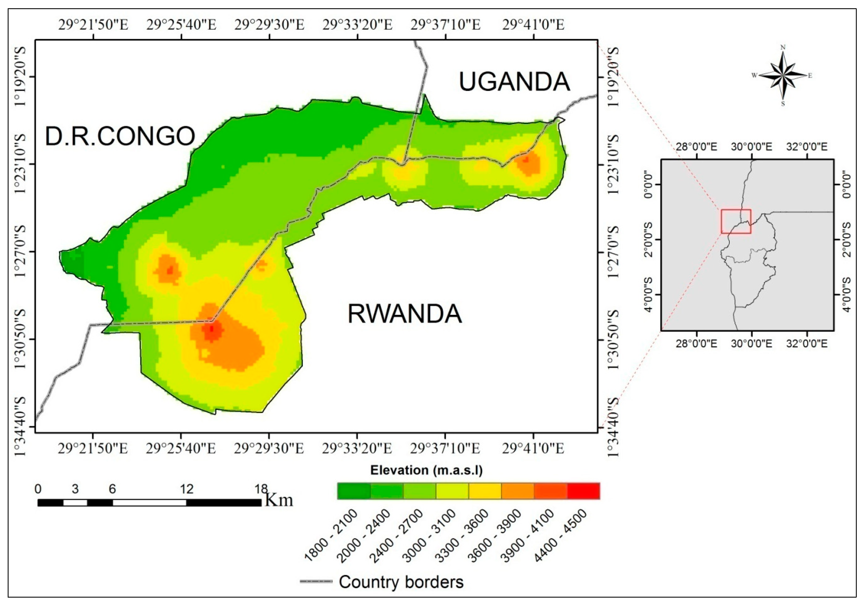
2.1. Study Area

The Virunga Volcanoes Massif is located in East-central Africa and lies within the border between Rwanda, the Democratic Republic of Congo (DRC), and Uganda [27]. This area is split into three National parks, namely the Volcanoes National Park (VNP) in Rwanda, the Mgahinga National Park in Uganda, and the Parc National des Virunga (NPVi) in DRC [29].
It is composed of a chain of five volcanoes covering a surface of 45,600 hectares (ha) (Figure 1) [23]. The topography is very steep with an elevation ranging from 1800 to 4500 m (Figure 1) [30] and the climate is characterized by a tropical climate [31]. Topographical complexity in this area results in diverse weather patterns which exert important influences on soil development and vegetation growth [32].
This study area has four climatic seasons in which long rainy (from February to May) and short rainy seasons (end-September to December) alternate, with two dry seasons known as long dry (from June to September) and short dry (Mid-December to Mid-February) [16]. The two rainy seasons correspond to the agricultural seasons, season A (September to December) and season B (January to May), respectively. Under normal circumstances, much rainfall is expected during the long rainy season [16].
This area is one with a rich biodiversity and is the unique home of rare mountain gorillas (Gorilla beringeri beringeri) and other apes. A census carried out in 2010 estimated that there were about 880 individual gorillas and showed that their numbers have been increasing at an annual rate of 3.7% since 2003 [33]. Vegetation cover forms a gorilla’s daily food intake and is used to create their nests. Moreover, vegetation in this area plays a primordial role in the local water cycle and this, in turn, affects the hydrological filtering and runoff processes.

2.2. Datasets

The spatial and temporal variations seen for vegetation growth are mainly monitored by means of Vegetation Indices (VI) and influences from various factors [34]. In this case, an evaluation of the effects of climatic and topographic factors on vegetation growth was assessed based on the relationship between these factors and NDVI, as illustrated in Table 1. The choice of these factors depended on the direct physical nature, size, and environmental nature of the Virunga Volcanoes Massif area.
MODIS NDVI, Landsat 8 Operational land imager (OLI) images, a Digital Elevation Model (DEM), global precipitation, and evapotranspiration (ET) were used as the primary data to compute the factors and indices listed in Table 1. The acquired MODIS NDVI data were 16-day composites with a 250 m spatial resolution. These NDVI data were freely available from NASA’s Terra satellite [35], for the acquisition period ranging from 2000 to 2014. Thus, 120 MODIS NDVI images (each year produced eight images) for the growing season A (from September to December) [36], over a period of 15 years, were used, given that season A is the most productive period of vegetation during the year. NDVI values of these four months of the growing season are enough to potentially show the patterns of the vegetation cover in this area [37].
Due to the insecurity in the region, there are few meteorological data available, and even when these data are available, they are often incomplete, as shown by the diagram of station data issued by the Rwanda Meteorological Agency [38]. In this case, we have utilized the satellite-derived precipitation data from 2000 to 2014, which were produced by the Global Precipitation Climatology Centre, available from the Earth System Research Laboratory with a 0.5 km spatial resolution [39].
MODIS global terrestrial evapotranspiration products indexed as NASA MOD16A2/A3 were downloaded from the University of Montana NTSG Lab’s website [40]. This dataset was calibrated to obtain land surface evapotranspiration values which accounted for all of the transpiration by vegetation and all of the evaporation from the canopy and soil surface. In addition, Landsat 8 OLI images acquired in 2014 at a 30 m resolution were downloaded from the USGS Earth Explorer (path: 172; row: 62) [41]. And were used to classify different vegetation types and to compute and estimate the Land Surface Temperature (LST), which was necessary to analyze the relationship between LST-emissivity, and vegetation growth and distribution in this area.
ASTER-derived DEM data, downloaded at a 30 m spatial resolution from USGS Earth Explorer [42], were used to estimate the elevation and to calculate aspect attributes. A shape file delimiting the study area was produced by the United Nations Environment Programme (UNEP) and was downloaded from Protected Planet website [43].

2.3. Data Processing

2.3.1. Data Pre-Processing

MODIS datasets, such as NDVI (MOD13Q1, 16-days composites) and ET (MOD16 A3) for the period from 2000 to 2014, and Landsat images were processed using ENVI software version 5.3 (Exelis Visual Information Solutions, Inc., a subsidiary of Harris Corporation, Boulder, CO, USA) and ArcGIS software version 10.2 (Environment Systems Research Institute (Esri) Inc., Redlands, CA, USA). The following steps were undertaken for data quality improvement: the downloaded MODIS NDVI and Global annual ET images were geographically reprojected to WGS_1984_UTM_zone_35S, which is the proper spatial reference of the study area.
Furthermore, these products were resampled and interpolated to match with the other datasets acquired at a 30 m spatial resolution, such as Landsat and DEM data, and to avoid pixel deterioration while clipping over the shape file. The MODIS NDVI data were then filtered using the Savitzky-Golay filtering method, to eliminate the effects from cloud contamination and residual atmospheric conditions [44]. Additionally, three steps were applied to improve the quality of Landsat data: (1) a radiometric calibration process was employed to account for sensor degradation; (2) FLAASH atmospheric correction was used to adjust the influence of water vapor, aerosols, ozone, and Rayleigh scattering; and (3) geometric correction using a registration image was applied to correct the images affected by the Scan Line Corrector (SCL-Off) [45].

2.3.2. Data Analysis

ArcGIS software version 10.2 (Environment Systems Research Institute (Esri) Inc., Redlands, CA, USA) was used for all analyses and calculations discussed herein. The mean values of NDVI were firstly calculated to form monthly averages, and thereafter, the calculated monthly NDVI values were used to calculate the annual mean NDVI. For climatic factors, the annual mean precipitation values were obtained by averaging the monthly data for each year, and the same process was applied to calculate the annual mean ET from 2000 to 2014. Additionally, all ET values were multiplied by 0.1, to obtain the real mean ET values in mm per year (mm/year), as suggested by Mu et al. [40]. The elevation was directly obtained from DEM data, while aspect values were derived from DEM data by using the Spatial Analyst tool in ArcGIS.The Maximum Likelihood supervised classification method using ENVI software version 5.3 (Exelis Visual Information Solutions, Inc., a subsidiary of Harris Corporation, Boulder, CO, USA) was applied, to produce the Land cover map for the Volcanoes massif region. During the classification process, to analyze the vegetation cover types of the Virunga Volcanoes Massif, we independently referred to 100 points provided by the Karisoke Research Center’s (KRC) botanical office, in order to classify and map vegetation types [28]. Eleven land cover classes were designed, of which nine were vegetation types, namely: bamboo, Hagenia-hypericum, Bush-ridge, Neubutonia, Alpine, Mimulopsis, Herbaceous, Meadow/savannah, and mixed forest respectively, followed by water, forming a crater lake on top of the Bisoke Volcano, and clouds. Since this area is the most cloud prone [46], persistent cloud cover has been designed as clouds during image processing.
Thereafter, we masked the no-vegetation covers (water and clouds), in order to check the important vegetation type distribution in this area. A total of 500 ground reference points acquired from field plotting sample points using a Global Positioning System (GPS: Garmin Map629sc with typical accurate to within 10 m) and Google earth (GE) were considered, to assess the accuracy of the classified land cover map of our study area. Out of the 500 ground truth points used, 430 of them were taken by GPS, while the 70 Ground Points taken from the inaccessible areas like on top of the volcanoes, in deep slopes, and those of water on top of the Bisoke volcano, were obtained from high resolution Google Earth (GE) images, conforming to the rule of thumb of at least 50 ground points per class using multinomial distribution observations [47].
The LST was calculated using a Landsat 8 OLI image of 2014, and the bands TIRS 10 and 11 were used to estimate the brightness temperature by applying the following mathematical equations with split-windows algorithms. The LST is equivalent to the difference between the land surface emissivity and brightness temperature, as suggested by Rozenstein, Q. et al. and Rajeshwani, A. et al. [48,49]. In this case, the Top of Atmospheric (TOA) spectral radiance (Lλ) was determined by multiplying multiplicative rescaling factors (3.342 × 10⁻⁴), in addition to the additive rescaling factor (0.1) of both TIR bands, which were provided in the metadata file as shown in Equation (1).
L λ = M L × Q cal + A L
where L λ is the Top of Atmospheric (TOA) spectral radiance in Watts/ (m2·srad·μm); M L is the band-specific multiplicative rescaling factors of TIR bands 10 and 11; Q cal is the band 10/11 image; and A L represents the additive rescaling factors for bands 10 and 11 [50].
The next process was to determine the Brightness Temperature (TB), which is the radiation of the radiance of the top of earth atmosphere. This calibration process was used to convert the thermal Digital Numbers (DN) of the thermal bands of TIR, to TB. The TB for both TIR bands was calculated by adopting the following formula:
TB = K 2 ln ( K 1 L λ + 1 )
where K 1 and K 2 are the thermal conversion constant and variables for both TIR of the bands, respectively. The K1 for band 10 is equal to 1321.08, whereas the K1 for Band11 is equal to 1201.14. The K2 values are 777.89 and 480.89 for band 10 and Band 11, respectively.
L λ represents the Top of Atmospheric spectral radiance.
The Land Surface Emissivity (LSE) was calculated and estimated by using the NDVI thresholds method (Formula (3), as follows:
LSE = ε s ( 1 FVC ) + ε v   ×   FVC
ε s and ε v are the soil and vegetation emissivity of the TIR bands, where the ε s value for band 10 is equal to 0.971 and is equal to 0.977 for band 11, and the ε v value for band 10 is 0.987 and 0.989 for band 11. FVC stands for the fractional vegetation cover, which was estimated for each pixel [51]. FVC was calculated as follows:
FVC = NDVI NDVIs NDVIv NDVIs
where NDVIs stands for the reclassified NDVI for Soil and NDVIv stands for the reclassified NDVI for Vegetation. In this case, we have used the mean NDVI calculated from 2000 to 2014.
Finally, the LST was calculated by applying the following formula:
LST = TB 10 + C 1 ( TB 10 TB 11 ) + C 2 ( TB 10 TB 11 ) 2 + C 0 + ( C 3 + C 4 W ) ( 1 ε ) + ( C 5 + C 6 W ) Δ ε
where LST is the Land Surface Temperature in degree Kelvin, multiplied by 273.15 to convert Kelvin to Celsius [52]; C0 to C6 represent the Split-Window Coefficient values (Table 2), as illustrated by Skokovic et al. [53] in their research; TB10 and TB11 are the Brightness Temperatures for Bands 10 and 11 in Kelvin; ε is the mean LSE of the TIR bands; W is the Atmospheric Water Vapor content; and Δ ε is the difference in the LSE.

2.3.3. Statistical Analysis and Relationship Calculations

The statistical values used to analyze changes in the NDVI in relation to elevation and aspect, were derived from the processed MODIS NDVI data using spatial analyst and spatial statistics tools in ArcGIS software. Therefore, the grid cells were used to depict the spatial patterns of NDVI, precipitation, LST, and ET towards the Virunga Volcanoes Massif, by creating a fishnet shapefile with 120 m grid cells. Then, NDVI, precipitation, LST, and ET maps were converted to 120 m grid cell maps. The values of each variable were intersected with the fishnet grid cells, and were dissolved to depict spatial patterns and effectively evaluate the spatial correlation between NDVI and the climatic factors (precipitation, LST, and ET) using the Geographically Weighted Regression (GWR) model.
In this case, the Moran’s Index was also employed to identify the existence and the intensity of the spatial autocorrelation of variables, while the GWR model explored and evaluated the important variations in spatial distribution and the relationship between spatial patterns of vegetation and climatic factors [54]. Thus, the GWR model indicated the spatial correlations between the variables by generating a series of location-specific parameters to visualize geographical interactions [54,55]. OriginPro version 9.0 (OriginLab, Northampton, MA, USA), a data analysis and graphing software, was used to graphically represent the results from an analysis of the variables.

3. Results

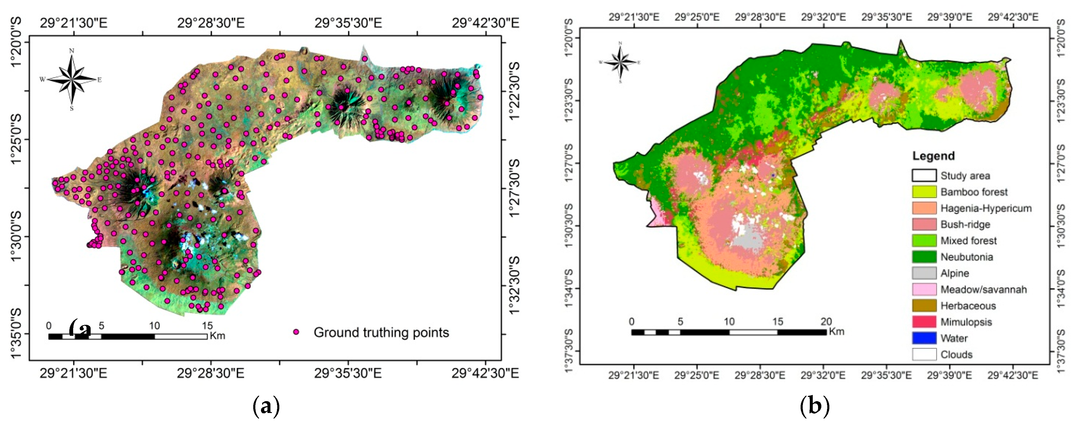
3.1. Vegetation Distribution over Virunga Volcanoes Massif

In order to estimate the vegetation distribution in the Virunga Volcanoes Massif, it is important to determine the vegetation types available, based on a land cover map. The image classification in the Virunga Volcanoes massif resulted in eleven land cover classes; nine of which were vegetation types, as shown in Figure 2b.
The classification accuracy assessment showed that the overall accuracy and Kappa coefficients of the LCLU map were 88% and 0.86%, respectively. Figure 2 shows the spatial distribution of the nine vegetation cover types in the Virunga Volcanoes massif. Statistically, the results indicate that Neubutonia occupies a preponderant place among all vegetation types, with a percentage area of 34.4%, while Meadow-Savannah extends over the smallest area (Table 3).

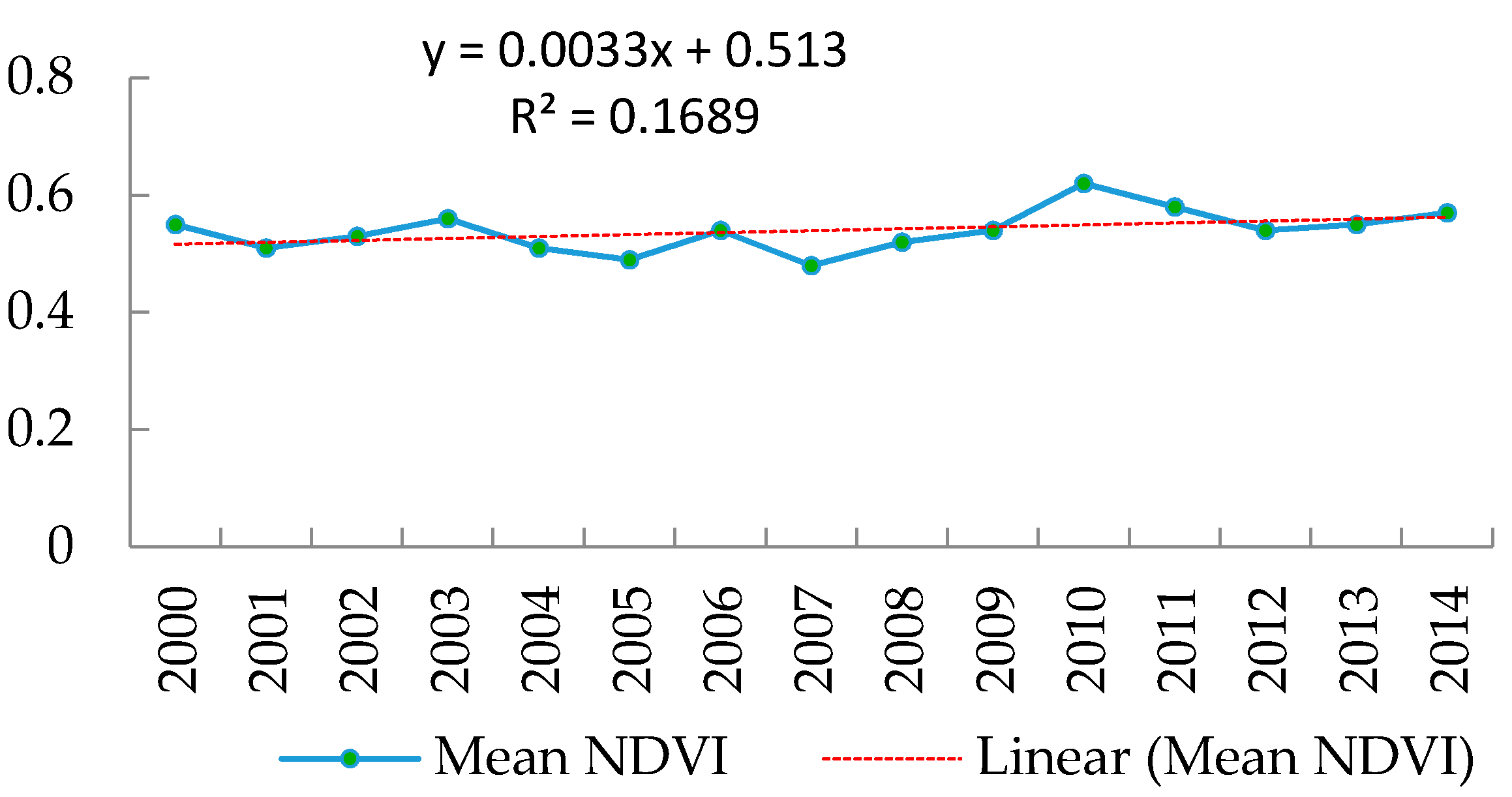
3.2. Vegetation Growth Analysis in Virunga Volcanoes Massif

The analysis of the general trend of vegetation changes from 2000 to 2014 in this area was performed by using NDVI. A one-dimensional linear regression method was used to analyze the changes. To avoid the influence of water bodies on the statistical averages, the negative pixel values were excluded from the calculations. Generally, negative NDVI values are found over water bodies which absorb the maximum portion of the Near Infrared light that falls on them [21,22]. The statistical evolution of NDVI values in the Virunga Volcanoes Massif indicated that the Mean NDVI from 2000 to 2014 varied between 0.48 and 0.62. A high vegetation growth was found in 2010 and 2011 at the maximum mean NDVI values of 0.62 and 0.58, respectively, while the minimum value recorded in 2007 was 0.48 (Figure 3).

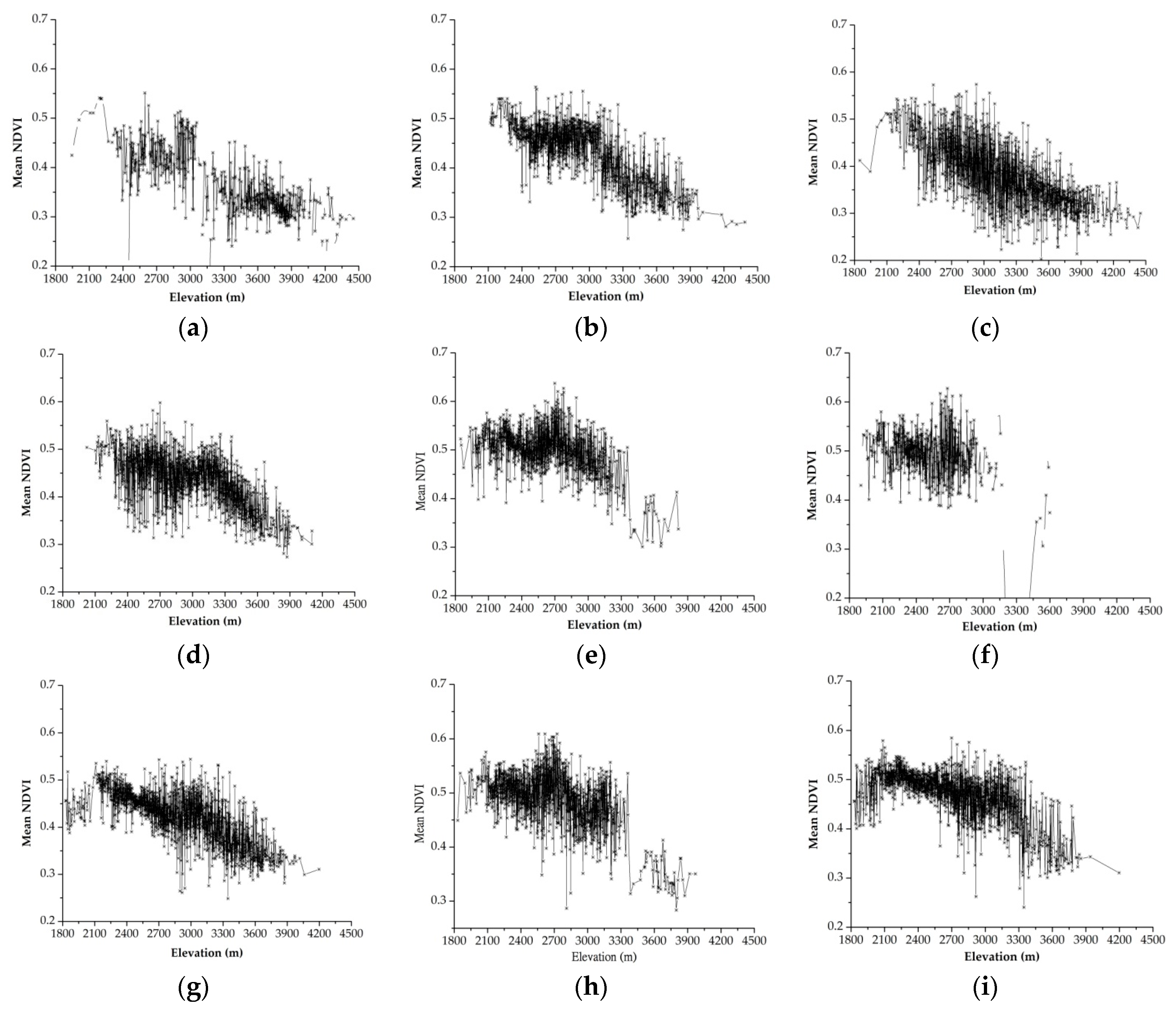
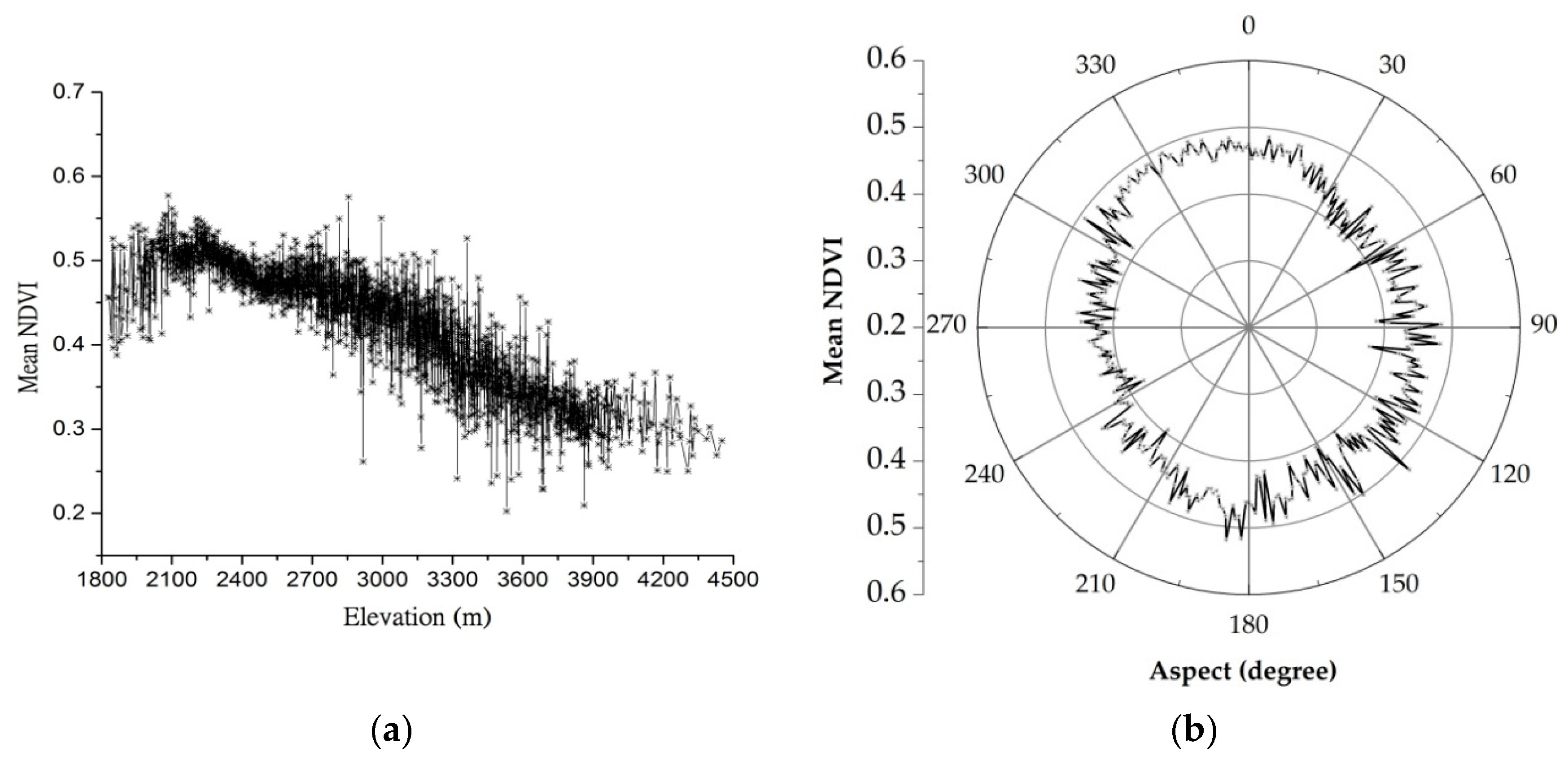
3.3. Geographical Distribution of Vegetation in the Virunga Volcanoes Massif

The geographical distribution of vegetation was analyzed by considering the topography with respect to two positions: (1) the vertical position that represents the spatial distribution of vegetation per elevation (in meters above sea level); and (2) the horizontal position that represents the spatial distribution of vegetation per aspect (in degrees). We divided elevation into a total of nine intervals of 300 m and aspect into 12 intervals of 30 degrees. A spatial analysis tool was used to match NDVI values with their corresponding elevation and aspect, in order to analyze their effects on vegetation dynamics in this mountainous area.
The results indicated that the high vegetation density was located at an elevation ranging from 2000 to 3900 m, while the lowest density was found at an elevation greater than 3900 m and less than 2000 m. Higher mean NDVI values were found at the elevation ranging from 2000 to 2400 m, while lower values were found at the top of the mountains (elevation ≥ 4000 m). These results indicate that the more the elevation increases, the more the mean NDVI decreases (Figure 4a). Also, the results highlighted that a high vegetation density was found in the North-East (22.5°–67.5°), from East (67.5°–112.5°) to South-East (112.5°–157.5°), and in the West (247.5°–292.5°). The highest mean NDVI values were located in the South-East (132°, 148°), South-West (182°, 186°), and North-West (309.5°–337.5°). The lowest were located in the North-East (60°), South-East (99°), South-West (243°–246°), and North-East (38°–47°), respectively (Figure 4b).

3.4. Analysis of Changes in Vegetation Growth and Spatial Distribution per Vegetation Types

The flux of vegetation density and spatial distribution per vegetation type was investigated. The results indicated that, for all types of vegetation, the highest vegetation growth was found at an elevation ranging from 1929 to 4200 m, whilst individually, Alpine vegetation varies from 2400 to 3000 m and from 3300 to 4000 m; Bamboo (2100–3900 m); Bush-ridge (2300–4000 m); Hagenia-Hypericum (2400–3900 m); Herbaceous (1900–3300 m); Meadow-savannah (1829–3000 m); Mimulopsis (1832–3900 m); and Mixed-forest (1829–4200 m).
The vegetation growth analysis per elevation (vertical) highlighted that Herbaceous vegetation had the highest mean NDVI (0.55–0.59) at an elevation ranging between 2600 and 2700 m, followed by Mimulopsis and Neubutonia, whose maximum mean NDVI was estimated from 0.55 to 0.59, at an elevation from 2650 to 2700 m. All others represented a mean NDVI maximum of up to 0.50, except for the Alpine and Bush-ridge, which exhibited lower mean NDVIs, as shown in Figure 5a–i.
The results revealed that the NW was the region characterized by optimal vegetation growth, where almost all the vegetation types had maximum mean NDVI values, as illustrated in Table 4. The findings indicated that, with respect to aspect, the vegetation growth for all vegetation types was found as being optimal towards Na, NW, and Nb directions. Therefore, it can be concluded that the vegetation types in the Virunga Volcanoes Massif represent absolute dependencies on the change in geographical positions in consideration with the changes in sun light angles, whereby higher mean NDVI values were located in the NW (337.5°) and N (356.5°) (Table 4).

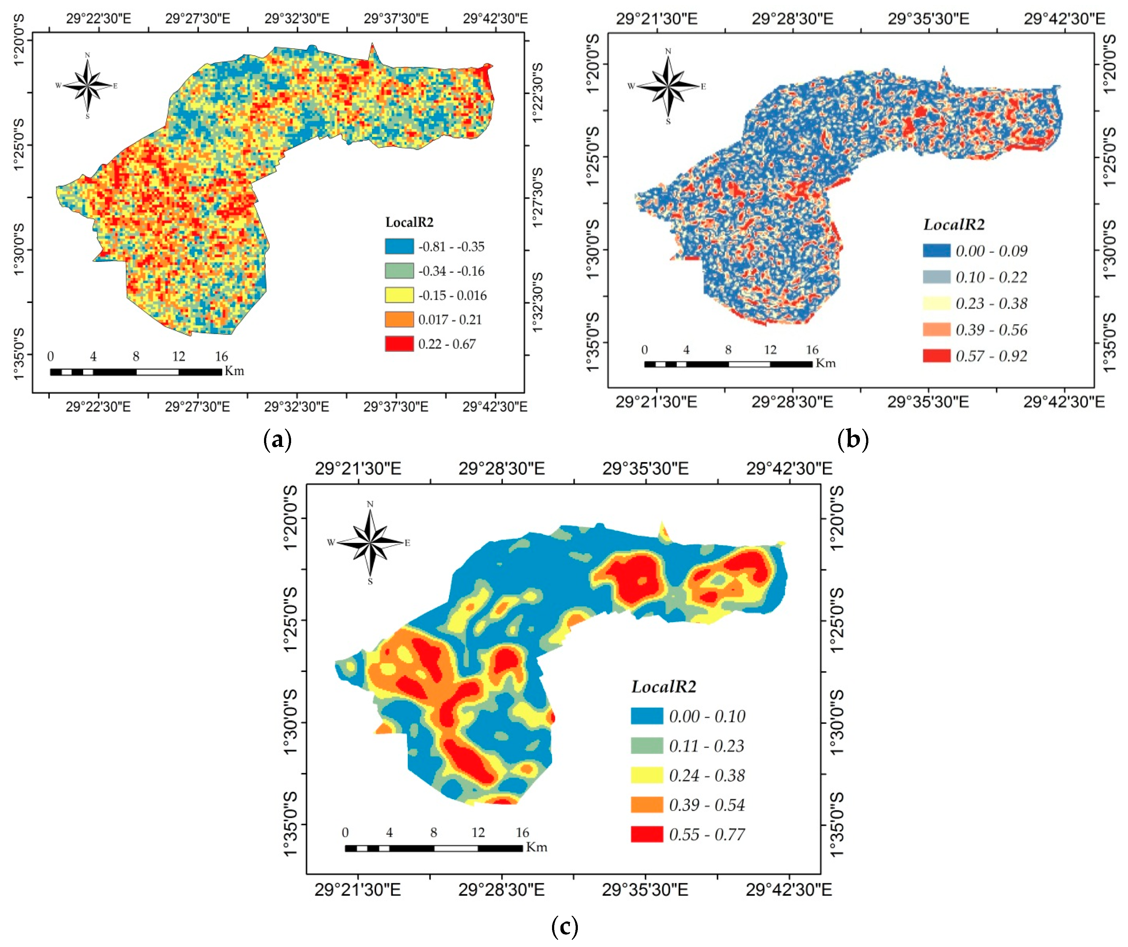
3.5. Analysis of Correlation between NDVI and Climatic Factors (Precipitation, LST and ET) in Virunga Volcanoes Massif

The Moran’s Index was employed to further understand the existence and integrity of the statistical autocorrelation between NDVI and climatic factors (precipitation, LST, and ET). The results revealed a high autocorrelation between NDVI and LST (Moran’s I = 0.99), and between NDVI and ET (Moran’s I = 0.96), at a 5% significance level (p-value < 0.05). The Moran’s I of 0.44 found between NDVI and precipitation indicated that precipitation was not correlated with NDVI in this area. The relationship between NDVI and climatic factors was also investigated using the GWR model, by focusing on their spatial distribution and local level spatial statistics. Therefore, the calculated grid cells were counted for about 31,737 for the entire area. For the GWR model, as a set of parameters [55], a local R squared parameter was chosen, among others, to evaluate the model’s performance. Thus, local R squared values were used to map the relationships between NDVI-Precipitation, NDVI-LST, and NDVI-ET (Figure 6).
The results showed that 22.03% of this area’s NDVI was not correlated with precipitation (absence of correlation), 67.44% indicated a negative correlation, while a positive correlation between the NDVI and precipitation was only found for about 10.6% of the entire Virunga Volcanoes Massif (Figure 6a).
The findings pointed out a significant correlation between NDVI and the LST with R2 = 81 and an adjusted R2 of 0.80. The results also indicated that over 42.75% of the Virunga Volcanoes Massif area’s NDVI was not correlated with LST, while a positive correlation was found over approximately 57.24% of the area, of which 23% had a weak correlation, 16.34% was fairly correlated, 11.08% was significantly correlated, and 6.82% was strongly correlated (Figure 6b).
In Figure 6c, the analysis of the correlation between the NDVI values and ET in the Virunga Volcanoes Massif indicated that an estimated 40.4% of the area’s vegetation was not correlated with ET, while about 59.6% was positively correlated with ET (R2 = 0.82 and R2 adjusted = 0.81). A total of 19% indicated a weak correlation, 15.22% showed a fair correlation, 14.05% showed a significant correlation, and 11.33% of the study area’s NDVI was strongly correlated with ET (Figure 6c).

4. Discussion

Vegetation growth and distribution has been studied and evaluated in this high altitude area by several researchers, such as Verbeken et al. [56], W. Robyns [57], and J. Lebrun and C. Marius [57], but different results and conclusions have been drawn. Referring to the results and conclusions established by Verbeken et al. [56] considering the climate, relief, soil, and volcanic activities, vegetation growth and distribution were influenced by topographical conditions. It was revealed that particular vegetation species were located in particular spots. Thus, the results indicated no growth of vegetation types at an elevation of less than 2100 m and greater than 3900 m, due to a lower temperature.
This was confirmed by the NDVI values represented by Alpine (Max mean NDVI of 0.32), with its density located at an elevation greater than 3600 m (Figure 5a), while the other vegetation types were characterized by an optimal vegetation growth of a mean NDVI greater than 0.59 at the elevation ranging from 2100 to 3300 m, except Meadow/savannah which varied in elevation range between 2100 to 3000 m (Figure 5). The evaluation for individual vegetation types according to aspect revealed that high vegetation growth was located in the North from 22.5° to 67.5° and from 337.5° to 359°, and in the NW at degrees from 292.5° and 337.5°.

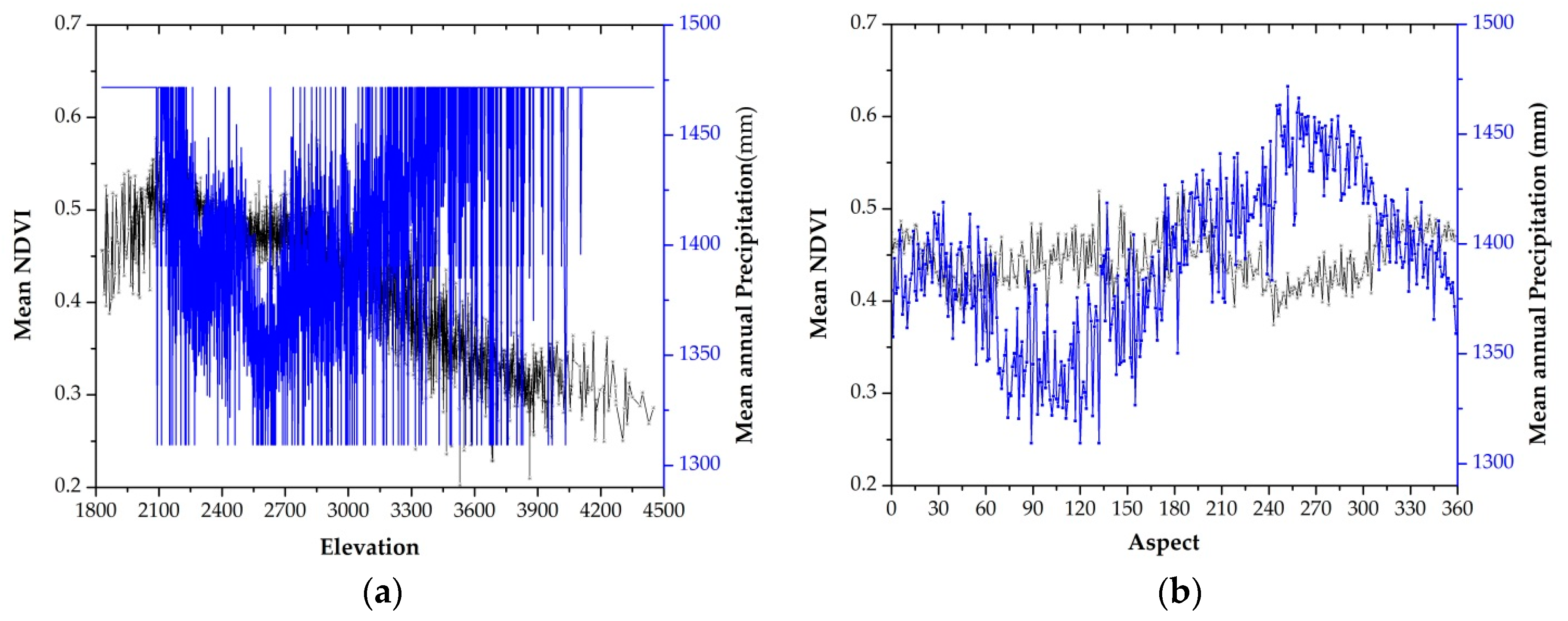
4.1. Impact of Precipitation on Vegetation Dynamics in Virunga Volcanoes Massif

The analysis of the relationship between precipitation and vegetation dynamics was carried out by considering MODIS NDVI and precipitation data from 2000 to 2014, where the mean annual precipitation was 1398.55 mm/year−1. The findings revealed that precipitation does not correlate with NDVI in the Virunga Volcanoes Massif (Figure 6a). It was shown that vegetation growth and distribution do not relate to the changes in precipitation, either vertically (elevation) or horizontally (aspect).

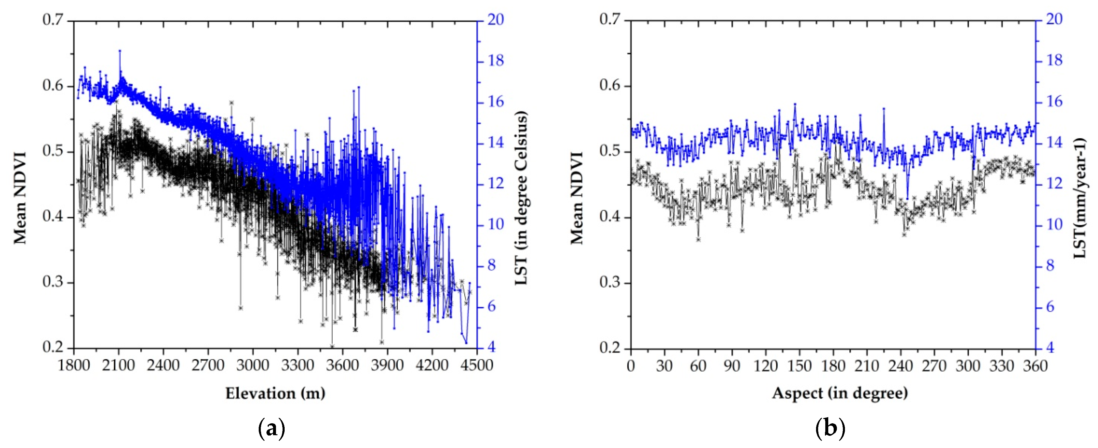
4.2. Impact of Land Surface Temperature (LST) on Vegetation Dynamics in Virunga Volcanoes Massif

Elevation and aspect are the main controllers of the spatial and pattern distribution of vegetation in the Virunga Volcanoes Massif. Nevertheless, the topographic factors and natural factors (precipitation & temperature) are included in this study to analyze their relationship and implications on vegetation growth and pattern distribution in this high altitude region. The LST was considered as an important microclimate factor to be used in our analysis and was well fitted with NDVI (R2 = 0.99 (Figure 6b)).
In this analysis, it was found that NDVI values vary with LST on elevation and aspect. The lowest mean LST (4 °C) was found at a top elevation of 4500 m and the highest (18.54 °C) was found at a middle elevation (2109 m) (Figure 7a). NDVI increases with LST along the decrease of elevation and reaches its peak (0.67) at 19 °C and 2100 m of elevation, before decreasing with the decrease in LST as the elevation contrarily increases. Thus, better vegetation growth was found in warm areas over the Virunga Volcanoes Massif (LST ≥ 18 °C), meaning that the shaded areas of the SE, SW, and NW were found to be the best to characterize the high vegetation growth (Figure 7b).

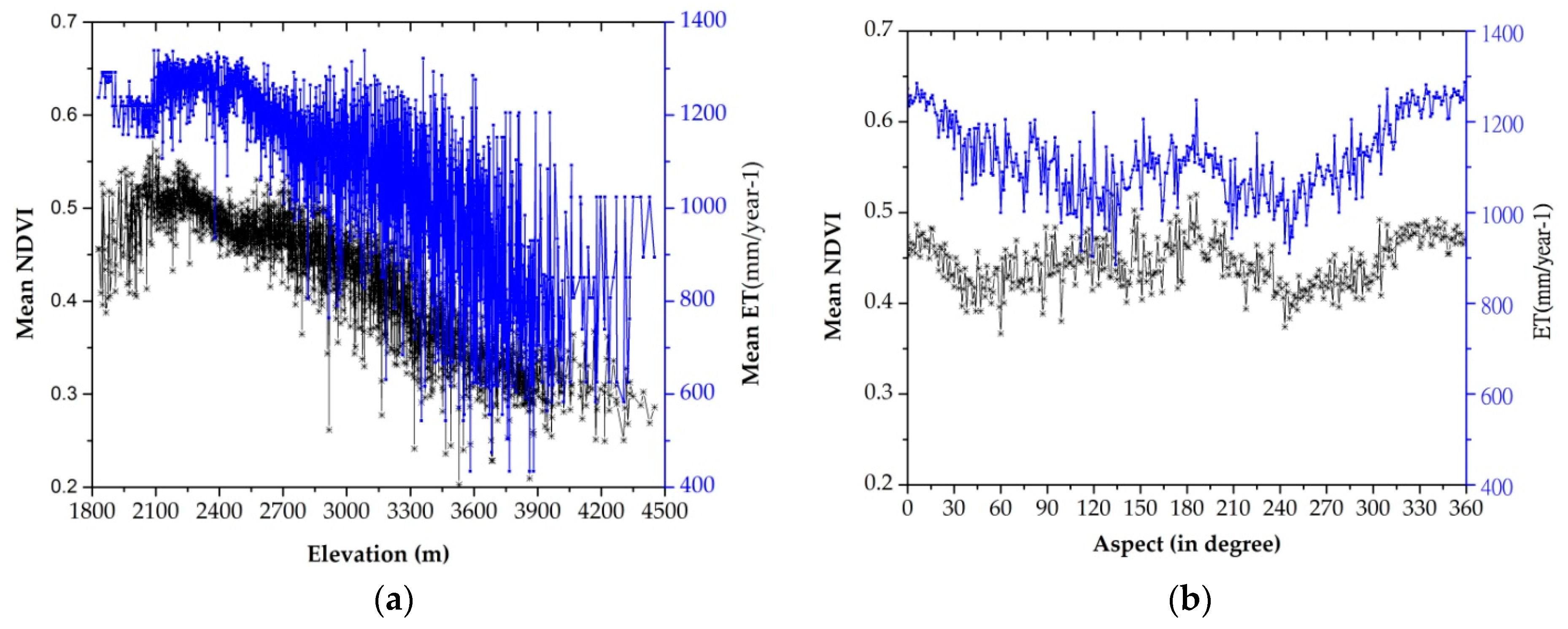
4.3. Impact of Evapotranspiration (ET) on Vegetation per Elevation and Aspect

The analysis of the variation of ET with the NDVI at a high altitude was found as a very important tool to evaluate the vegetation dynamics. The results obtained from the analysis showed that, in the Virunga Volcanoes Massif, NDVI changes were governed by changes in ET. Thus, the increase of NDVI is proportional to the increase of ET over elevation and aspect. In this area, ET varies with elevation and a higher ET was concentrated at a lower elevation. Additionally, both the highest annual mean ET and NDVI values were located between 2100 and 2500 m (Figure 8a). This is emphasized by the results reported earlier on the ET and NDVI relationship per aspect, where we found that the increase in NDVI was related to the increase in ET. Meanwhile, the increased ET in the shaded area was the most important factor for vegetation growth in the Virunga Volcanoes Massif area. Thus, the maximum NDVI (>0.6) was found where the mean ET was maximal (1286 mm/year−1), specifically in the North (356°–359°) (Figure 8b). This phenomenon proved the high correlation between ET and NDVI.
Owing to its geographical position, the Virunga Volcanoes massif area holds an equatorial climate which implies a moderate temperature >25 °C and high amount of rainfall, with an annual mean of about 1398.55 mm/year−1. Heavy rainfall occurs twice a year in April and October, as reported by Verbeken et al. [56], where the mean annual precipitation varies from 1300 to 1471 mm/yr−1. Consequently, the vulnerability of vegetation to excessive rainfall is very high. This increased vulnerability is translated into the fact that changes in vegetation growth were not associated with changes in precipitation R2 = 0.34 (Figure 6a). This was also suggested by D.P. Watts [58] in his results on seasonality in the ecology and life styles of mountain gorillas (Gorilla gorilla beringei), stating that no correlation was found between vegetation change and rainfall in this area (R2 = 0.48). The variation in the NDVI values was totally independent from the variations in precipitation at all levels of elevation and aspect angles (Figure 7).
On the contrary, vegetation growth and distribution were highly linked with LST (R2 = 99) and evapotranspiration (R2 = 96). The LST varies from 4 to 24.5 °C, while the evapotranspiration from soil evaporation and plants’ transpiration in this area varies from 400 to 1370 mm/year−1. These results highlighted that the peak mean NDVI value (0.59) was found at the peak value of the mean LST (19 °C) (Figure 8). The maximum mean NDVI values (>0.55) were found where the ET was greater than 1300 mm/year−1 (Figure 9).
The analysis highlighted that the NDVI increases with the climatic factors (LST and ET) and decreases with the increase of elevation. Both the NDVI and climatic factors (ET, precipitation, and LST) manifested trends of increase in the SE, SW, and NW, as can be seen in Figure 8 and Figure 9. It was clearly shown that greater NDVI values or better growth conditions for vegetation occurred in places where the land surface temperature fell within the range of 10 °C to 18 °C. High levels of associability between the land surface temperature and vegetation were detected at an elevation between 2100 and 3900 m and in the shady area (SE, SW, and NW).
Among the climate factors, precipitation and temperature were regarded as the two most important climatic factors controlling the differences in the Earth’s vegetation cover, by affecting the growth rate and plant reproduction, in combination with evapotranspiration [59]. In this study, however, only LST was found to be the most determinant factor, driving vegetation dynamics in the Virunga Volcanoes Massif region. In other areas, Hemp, A. reported that soil moisture was the most controlling climatic factor in the lower to middle altitudes of mount Kilimanjaro [60].
Similar works were conducted in arid and semi-arid regions, such as the Qilian mountain in China [61] and the Darab mountain in Iran [62], and found that in arid/semi-arid zones, vegetation growth and distribution highly depend on the amount of precipitation, while in the Tropical zone, vegetation does not depend on precipitation. Commonly, vegetation change depends on temperature and is controlled by elevation and aspect. The more that the vegetation increases, the more that it is exposed to high evaporation and transpiration from the soil moisture; which tends to explain why optimal vegetation growth can been seen in the SE (132°, 148°), SW (182°, 186°), and NW (309.5°–337.5°), in the shady areas. Therefore, it can be inferred that vegetation increases with the increase of evapotranspiration, due to poor sun light reflectance.

5. Conclusions

This study evaluated the vegetation growth patterns and the spatial distribution in the Virunga Volcanoes Massif by means of remotely sensed data, by considering the vegetation cover types. The growing season (season A) was considered as the optimal period to indicate the change of vegetation in this area. Basing on the results obtained from the analysis of NDVI variability per vegetation type within the last 15 years, it is indicated that elevation and aspect were the main controllers of vegetation growth and spatial distribution, along with the variation in precipitation, LST, and ET. It was found that the optimal vegetation growth occurred at an elevation between 2000 to 3900 m, with mean NDVI values higher than 0.5 at around 2100 and 2800 m. The greater vegetation growth with (NDVI ≥ 0.56) was found in the SE (132°, 148°), SW (182°, 186°), and NW (309.5°–337.5°) (Figure 4b). Thus, it was found that better vegetation growth occurs over lower elevation ranges and shady areas.
The analysis revealed that vegetation growth is more sensitive to elevation in this area and the rate change in mean NDVI values varies more gently in lower-to-mid elevation areas (at elevation between 2000 and 3000 m) than in higher elevation (at <4000 m). The annual mean precipitation (1398.55 mm/year−1), LST (≥18 °C), and ET (1286 mm/year−1) were found to provide optimal conditions for vegetation growth in the Virunga Volcanoes Massif. Except for precipitation, LST and ET were found to be the main climatic factors controlling vegetation dynamics in this area. It was found that vegetation dynamics in the Virunga Volcanoes Massif were more driven by the solar radiation cumulates or the differences in LST and land surface evaporation, and transpiration from the plants’ canopy. The findings provided the current state of vegetation growth and spatial distribution, while helping to disentangle the impacts of climatic and topographical factors’ interactions on vegetation. This information is significantly helpful to the Virunga, Mgahinga, and Volcanoes National Parks management in terms of wildlife conservation, vegetation, and environmental regeneration, as well as for species analysis and ecological research.

Acknowledgements

We would like to thank the United States Geological Survey and the NASA team for the provision of data. The authors would like also to thank the anonymous reviewers and Editor whose constructive comments and suggestions have helped to improve the quality of this manuscript.

Author Contributions

Alphonse Kayiranga designed the research, processed data, and wrote the manuscript; Christophe Mupenzi, Fidele Karamage, Felix Ndayisaba, Lamek Nahayo, Jean Baptiste Nsengiyumva, and Enan Muhire Nyesheja provided technical assistance. All authors contributed to the completion of this research by contributing valuable ideas.

Conflicts of Interest

The authors declare no conflict of interest.

References

  1. Hong, W.; Jiang, R.; Yang, C.; Zhang, F.; Su, M.; Liao, Q. Establishing an ecological vulnerability assessment indicator system for spatial recognition and management of ecologically vulnerable areas in highly urbanized regions: A case study of shenzhen, China. Ecol. Indic. 2016, 69, 540–547. [Google Scholar] [CrossRef]
  2. Chan, K.M.; Shaw, M.R.; Cameron, D.R.; Underwood, E.C.; Daily, G.C. Conservation planning for ecosystem services. PLoS Biol. 2006, 4, e379. [Google Scholar] [CrossRef] [PubMed]
  3. Ribeiro, E.; Santos, B.A.; Arroyo-Rodríguez, V.; Tabarelli, M.; Souza, G.; Leal, I.R. Phylogenetic impoverishment of plant communities following chronic human disturbances in the brazilian caatinga. Ecology 2016, 97, 1583–1592. [Google Scholar] [CrossRef] [PubMed]
  4. Singh, P.; Kainthola, A.; Panthee, S.; Singh, T. Rockfall analysis along transportation corridors in high hill slopes. Environ. Earth Sci. 2016, 75, 1–11. [Google Scholar] [CrossRef]
  5. Brang, P.; Schonenberger, W.; Ott, E.; Gardner, B. 3: Forests as Protection from Natural Hazards; John Wiley & Sons, Inc.: New York, NY, USA, 2001. [Google Scholar]
  6. Suding, K.N.; Farrer, E.C.; King, A.J.; Kueppers, L.; Spasojevic, M.J. Vegetation change at high elevation: Scale dependence and interactive effects on niwot ridge. Plant Ecol. Divers. 2015, 8, 713–725. [Google Scholar] [CrossRef]
  7. Bai, Y.; Broersma, K.; Thompson, D.; Ross, T.J. Landscape-level dynamics of grassland-forest transitions in british columbia. J. Range Manag. 2004, 57, 66–75. [Google Scholar] [CrossRef]
  8. Jin, X.; Zhang, Y.; Schaepman, M.; Clevers, J.; Su, Z. Impact of elevation and aspect on the spatial distribution of vegetation in the qilian mountain area with remote sensing data. Int. Arch. Photogramm. Remote Sens. Spat. Inf. Sci. 2008, 37, 1385–1390. [Google Scholar]
  9. Bachmair, S.; Weiler, M. Hillslope characteristics as controls of subsurface flow variability. Hydrol. Earth Syst. Sci. 2012, 16, 3699–3715. [Google Scholar] [CrossRef] [Green Version]
  10. Wood, S.W.; Murphy, B.P.; Bowman, D.M. Firescape ecology: How topography determines the contrasting distribution of fire and rain forest in the south-west of the tasmanian wilderness world heritage area. J. Biogeogr. 2011, 38, 1807–1820. [Google Scholar] [CrossRef]
  11. Hwang, T.; Song, C.; Vose, J.M.; Band, L.E. Topography-mediated controls on local vegetation phenology estimated from modis vegetation index. Landsc. Ecol. 2011, 26, 541–556. [Google Scholar] [CrossRef]
  12. Hession, S.; Moore, N. A spatial regression analysis of the influence of topography on monthly rainfall in east africa. Int. J. Climatol. 2011, 31, 1440–1456. [Google Scholar] [CrossRef]
  13. Couteron, P.; Hunke, P.; Bellot, J.; Estrany, J.; Martínez-Carreras, N.; Mueller, E.N.; Papanastasis, V.P.; Parmenter, R.R.; Wainwright, J. Characterizing patterns. In Patterns of Land Degradation in Drylands; Springer: New York, NY, USA, 2014; pp. 211–245. [Google Scholar]
  14. Purkis, S.J.; Klemas, V.V. Remote Sensing and Global Environmental Change; John Wiley & Sons: New York, NY, USA, 2011. [Google Scholar]
  15. Yang, X.; Chen, L. Using multi-temporal remote sensor imagery to detect earthquake-triggered landslides. Int. J. Appl. Earth Obs. Geoinf. 2010, 12, 487–495. [Google Scholar] [CrossRef]
  16. Ndayisaba, F.; Guo, H.; Bao, A.; Guo, H.; Karamage, F.; Kayiranga, A. Understanding the spatial temporal vegetation dynamics in rwanda. Remote Sens. 2016, 8, 129. [Google Scholar] [CrossRef]
  17. Matsushita, B.; Yang, W.; Chen, J.; Onda, Y.; Qiu, G. Sensitivity of the enhanced vegetation index (EVI) and normalized difference vegetation index (NDVI) to topographic effects: A case study in high-density cypress forest. Sensors 2007, 7, 2636–2651. [Google Scholar] [CrossRef]
  18. De Jong, R.; de Bruin, S.; de Wit, A.; Schaepman, M.E.; Dent, D.L. Analysis of monotonic greening and browning trends from global ndvi time-series. Remote Sens. Environ. 2011, 115, 692–702. [Google Scholar] [CrossRef] [Green Version]
  19. Motohka, T.; Nasahara, K.N.; Oguma, H.; Tsuchida, S. Applicability of green-red vegetation index for remote sensing of vegetation phenology. Remote Sens. 2010, 2, 2369–2387. [Google Scholar] [CrossRef]
  20. Jia, K.; Liang, S.; Wei, X.; Yao, Y.; Su, Y.; Jiang, B.; Wang, X. Land cover classification of landsat data with phenological features extracted from time series modis ndvi data. Remote Sens. 2014, 6, 11518–11532. [Google Scholar] [CrossRef]
  21. Dulamsuren, C.; Khishigjargal, M.; Leuschner, C.; Hauck, M. Response of tree-ring width to climate warming and selective logging in larch forests of the mongolian altai. J. Plant Ecol. 2014, 7, 24–38. [Google Scholar] [CrossRef]
  22. Yospin, G.I.; Wood, S.W.; Holz, A.; Bowman, D.M.; Keane, R.E.; Whitlock, C. Modeling vegetation mosaics in sub-alpine tasmania under various fire regimes. Model. Earth Syst. Environ. 2015, 1, 1–10. [Google Scholar] [CrossRef]
  23. Sheil, D.; Ducey, M.; Ssali, F.; Ngubwagye, J.M.; van Heist, M.; Ezuma, P. Bamboo for people, mountain gorillas, and golden monkeys: Evaluating harvest and conservation trade-offs and synergies in the virunga volcanoes. For. Ecol. Manag. 2012, 267, 163–171. [Google Scholar] [CrossRef]
  24. Galbany, J.; Imanizabayo, O.; Romero, A.; Vecellio, V.; Glowacka, H.; Cranfield, M.R.; Bromage, T.G.; Mudakikwa, A.; Stoinski, T.S.; McFarlin, S.C. Tooth wear and feeding ecology in mountain gorillas from volcanoes national park, rwanda. Am. J. Phys. Anthropol. 2016, 159, 457–465. [Google Scholar] [CrossRef] [PubMed]
  25. Smets, B.; Kervyn, M.; d’Oreye, N.; Kervyn, F. Spatio-temporal dynamics of eruptions in a youthful extensional setting: Insights from Nyamulagira Volcano (DR Congo), in the western branch of the East African Rift. Earth-Sci. Rev. 2015, 150, 305–328. [Google Scholar] [CrossRef]
  26. Owiunji, I.; Nkuutu, D.; Kujirakwinja, D.; Liengola, I.; Plumptre, A.; Nsanzurwimo, A.; Fawcett, K.; Gray, M.; McNeilage, A. The Biodiversity of the Virunga Volcanoes; Unpublished Report; Wildlife Conservation Society: Bronx, NY, USA, 2005. [Google Scholar]
  27. Van Gils, H.; Kayijamahe, E. Sharing natural resources: Mountain gorillas and people in the Parc National Des Volcans, Rwanda. Afr. J. Ecol. 2010, 48, 621–627. [Google Scholar] [CrossRef]
  28. Kayijamahe, E. Spatial Modelling of Mountain Gorilla (Gorilla Beringei Beringei) Habitat Suitability and Human Impact. Master’s Thesis, International Institute of Geo-Information Science and Earth Observation, Enschede, The Netherlands, 2008. [Google Scholar]
  29. Maekawa, M.; Lanjouw, A.; Rutagarama, E.; Sharp, D. Mountain gorilla tourism generating wealth and peace in post-conflict Rwanda. In Natural Resources Forum; Wiley Online Library: Hoboken, NJ, USA, 2013; pp. 127–137. [Google Scholar]
  30. Plumptre, A.J.; Kujirakwinja, D.; Treves, A.; Owiunji, I.; Rainer, H. Transboundary conservation in the greater Virunga landscape: Its importance for landscape species. Biol. Conserv. 2007, 134, 279–287. [Google Scholar] [CrossRef]
  31. Musana, A.; Mutuyeyezu, A. Impact of Climate Change and Climate Variability on Altitudinal Ranging Movements of Mountain Gorillas in Volcanoes National Park, Rwanda; Externship Report; The International START Secretariat: Washington, DC, USA, 2011. [Google Scholar]
  32. Karamage, F.; Zhang, C.; Ndayisaba, F.; Shao, H.; Kayiranga, A.; Fang, X.; Nahayo, L.; Muhire Nyesheja, E.; Tian, G. Extent of cropland and related soil erosion risk in Rwanda. Sustainability 2016, 8, 609. [Google Scholar] [CrossRef]
  33. Gray, M.; Roy, J.; Vigilant, L.; Fawcett, K.; Basabose, A.; Cranfield, M.; Uwingeli, P.; Mburanumwe, I.; Kagoda, E.; Robbins, M.M. Genetic census reveals increased but uneven growth of a critically endangered mountain gorilla population. Biol. Conserv. 2013, 158, 230–238. [Google Scholar] [CrossRef]
  34. Dobos, E.; Micheli, E.; Baumgardner, M.F.; Biehl, L.; Helt, T. Use of combined digital elevation model and satellite radiometric data for regional soil mapping. Geoderma 2000, 97, 367–391. [Google Scholar] [CrossRef]
  35. NDVI Data from NASA’s Terra Satellite. Available online: http://ladsweb.nascom.nasa.gov/data/html (accessed on 15 September 2016).
  36. Diao, X.; Hazell, P.B.; Resnick, D.; Thurlow, J. The Role of Agriculture in Development: Implications for Sub-Saharan Africa; International Food Policy Research Institute: Washington, DC, USA, 2007; Volume 153. [Google Scholar]
  37. Pettorelli, N.; Vik, J.O.; Mysterud, A.; Gaillard, J.-M.; Tucker, C.J.; Stenseth, N.C. Using the satellite-derived ndvi to assess ecological responses to environmental change. Trends Ecol. Evol. 2005, 20, 503–510. [Google Scholar] [CrossRef] [PubMed]
  38. Agency, R.M. Climatology of Rwanda. Available online: http://www.meteorwanda.gov.rw/index.php?id=2 (accessed on 15 September 2016).
  39. Global Precipitation Climatology Centre, E.S.R.L. Global precipitation data. Available online: www.esrl.naoo.gov (accessed on 16 September 2016).
  40. Mu, Q.; Zhao, M.; Running, S.W. Improvements to a modis global terrestrial evapotranspiration algorithm. Remote Sens. Environ. 2011, 115, 1781–1800. [Google Scholar] [CrossRef]
  41. USGS. USGS global visualization viewer: Earth resources observation and science center (eros). Available online: http://www.glovis.usgs.gov/index.shtml (accessed on 20 September 2016).
  42. USGS. U.S. Geological survey earthexplorer (ee) tool. Available online: http://www.earthexplorer.usgs.gov/ (accessed on 21 September 2016).
  43. Protected Planet. Available online: http://www.protectedplanet.net (accessed on 15 September 2016).
  44. Piao, S.; Mohammat, A.; Fang, J.; Cai, Q.; Feng, J. NDVI-based increase in growth of temperate grasslands and its responses to climate changes in China. Glob. Environ. Chang. 2006, 16, 340–348. [Google Scholar] [CrossRef]
  45. Kayiranga, A.; Kurban, A.; Ndayisaba, F.; Nahayo, L.; Karamage, F.; Ablekim, A.; Li, H.; Ilniyaz, O. Monitoring forest cover change and fragmentation using remote sensing and landscape metrics in Nyungwe-Kibira park. J. Geosci. Environ. Prot. 2016, 4, 13. [Google Scholar] [CrossRef]
  46. Basnet, B.; Vodacek, A. Tracking land use/land cover dynamics in cloud prone areas using moderate resolution satellite data: A case study in Central Africa. Remote Sens. 2015, 7, 6683–6709. [Google Scholar] [CrossRef]
  47. Congalton, R.G.; Green, K. Assessing the Accuracy of Remotely Sensed Data: Principles and Practices; CRC Press: Boca Raton, FL, USA, 2008. [Google Scholar]
  48. Rozenstein, O.; Qin, Z.; Derimian, Y.; Karnieli, A. Derivation of land surface temperature for landsat-8 TIRS using a split window algorithm. Sensors 2014, 14, 5768–5780. [Google Scholar] [CrossRef] [PubMed]
  49. Rajeshwari, A.; Mani, N. Estimation of land surface temperature of dindigul district using landsat 8 data. Int. J. Res. Eng. Technol. 2014, 3, 122–126. [Google Scholar]
  50. Yu, X.; Guo, X.; Wu, Z. Land surface temperature retrieval from landsat 8 TIRS—Comparison between radiative transfer equation-based method, split window algorithm and single channel method. Remote Sens. 2014, 6, 9829–9852. [Google Scholar] [CrossRef]
  51. Zhang, X.; Liao, C.; Li, J.; Sun, Q. Fractional vegetation cover estimation in arid and semi-arid environments using HJ-1 satellite hyperspectral data. Int. J. Appl. Earth Obs. Geoinf. 2013, 21, 506–512. [Google Scholar] [CrossRef]
  52. Rogan, J.; Ziemer, M.; Martin, D.; Ratick, S.; Cuba, N.; DeLauer, V. The impact of tree cover loss on land surface temperature: A case study of central massachusetts using landsat thematic mapper thermal data. Appl. Geogr. 2013, 45, 49–57. [Google Scholar] [CrossRef]
  53. Skoković, D.; Sobrino, J.; Jimenez-Munoz, J.; Soria, G.; Julien, Y.; Mattar, C.; Cristóbal, J. Calibration and Validation of Land Surface Temperature for Landsat8-TIRS Sensor. 2014. Available online: https://earth.esa.int/documents/700255/2126408/ESA_Lpve_Sobrino_2014a.pdf (accessed on 22 March 2017).
  54. Abliz, A.; Tiyip, T.; Ghulam, A.; Halik, Ü.; Ding, J.-L.; Sawut, M.; Zhang, F.; Nurmemet, I.; Abliz, A. Effects of shallow groundwater table and salinity on soil salt dynamics in the Keriya Oasis, Northwestern China. Environ. Earth Sci. 2016, 75, 1–15. [Google Scholar] [CrossRef]
  55. Maimaitijiang, M.; Ghulam, A.; Sandoval, J.O.; Maimaitiyiming, M. Drivers of land cover and land use changes in st. Louis metropolitan area over the past 40 years characterized by remote sensing and census population data. Int. J. Appl. Earth Obs. Geoinf. 2015, 35, 161–174. [Google Scholar] [CrossRef]
  56. Verbeken, J.; De Temmerman, L.; Goossens, R.; De Maeyer, P.; Lavreau, J. Classification of the vegetation in the Virunga National Park (DR Congo) by integrating past mission reports into landsat-TM and terra aster sensors. In Proceedings of the 24th EARSeL Symposium ‘New Strategies for European Remote Sensing’, Dubrovnik, Croatia, 24–27 May 2004; pp. 11–16.
  57. Robijns, W. Vegetatiebeelden der Nationale Parken van Belgisch Congo. Serie 1. Het Nationaal Albert Park; Instituut der National Parken van Belgisch Congo: Brussels, belgium, 1937. [Google Scholar]
  58. Watts, D.P. Seasonality in the ecology and life histories of mountain gorillas (gorilla gorilla beringei). Int. J. Primatol. 1998, 19, 929–948. [Google Scholar] [CrossRef]
  59. Wang, J.; Price, K.; Rich, P. Spatial patterns of NDVI in response to precipitation and temperature in the central great plains. Int. J. Remote Sens. 2001, 22, 3827–3844. [Google Scholar] [CrossRef]
  60. Hemp, A. Continuum or zonation? Altitudinal gradients in the forest vegetation of mt. Kilimanjaro. Plant Ecol. 2006, 184, 27–42. [Google Scholar] [CrossRef]
  61. Jin, X.; Wan, L.; Zhang, Y.-K.; Hu, G.; Schaepman, M.; Clevers, J.; Su, Z.B. Quantification of spatial distribution of vegetation in the Qilian mountain area with MODIS NDVI. Int. J. Remote Sens. 2009, 30, 5751–5766. [Google Scholar] [CrossRef]
  62. Mokarram, M.; Sathyamoorthy, D. Modeling the relationship between elevation, aspect and spatial distribution of vegetation in the Darab mountain, Iran using remote sensing data. Model. Earth Syst. Environ. 2015, 1, 1–6. [Google Scholar] [CrossRef]
Figure 1. A map showing the location of the study area.
Geosciences 07 00017 g001
Figure 2. (a) Landsat image of the Virunga Volcanoes massif displayed in bands 4 (Near Infrared), 5 (SW Infrared), and 2 (Green), respectively. (b) Land cover map representing vegetation cover types and distribution within the Virunga Volcanoes massif.
Geosciences 07 00017 g002
Figure 3. Growing Season mean NDVI changes in the Virunga Volcanoes massif from 2000 to 2014.
Geosciences 07 00017 g003
Figure 4. Scatter plot (spline connected) showing the Variation of NDVI (a) per elevation (Vertical) and (b) a Rose chart showing the variation of NDVI per aspect (horizontal) in the Virunga-Volcanoes massif.
Geosciences 07 00017 g004
Figure 5. The scatter plots (spline connected) show the density and distribution of each vegetation type per elevation over the Virunga Volcanoes Massif; (a) Alpine; (b) Bamboo; (c) Bush-ridge; (d) Hagenia-Hypericum; (e) Herbaceous; (f) Meadow-Savannah; (g) Mixed-forest; (h) Mimulopsis; and (i) Neubutonia.
Geosciences 07 00017 g005
Figure 6. Spatial variability of the GWR model output, the coefficient of determination (Local R2), results: (a) Relationship between NDVI and precipitation; (b) NDVI and LST; and (c) NDVI and ET.
Geosciences 07 00017 g006
Figure 7. Scatter plot (spline connected) showing the change of NDVI with the mean annual precipitation per elevation (a) and per aspect (b).
Geosciences 07 00017 g007
Figure 8. Scatter plot (spline connected) showing the change of NDVI with the annual LST and averaged per elevation (a) and per aspect (b).
Geosciences 07 00017 g008
Figure 9. Scatter plot (spline connected) showing the change of NDVI with the mean annual ET per elevation (a) and per aspect (b).
Geosciences 07 00017 g009
Table 1. Factors and vegetation index considered in this study.
Climate FactorsTopography Vegetation Indices (VIs)
Precipitation (Rainfall)Aspect calculated from DEMNormalized Difference Vegetation-
Land Surface Temperature ElevationIndex (NDVI)
Evapotranspiration--
Table 2. Split-Window Coefficient values
C0C1C2C3C4C5C6
−0.2681.3780.18354.3−2.238−129.216.4
Table 3. Vegetation types in the Virunga Volcanoes and their specific area of coverage.
Vegetation Types%Area (Sq.km)
Bamboo Forest10.774894.81
Hagenia-Hypericum11.175075.98
Bush ridge14.586626.79
Mixed forest15.527053.04
Neubutonia33.9715,442.10
Alpine1.91869.77
Meadow/savannah1.08491.14
Herbaceous5.152339.76
Mimulopsis3.871758.71
Table 4. Change of mean and standard deviation of NDVI per aspect and per vegetation cover type.
Veg. TypeNDVINaNEESESSWWNWNb
BambooMean0.510.480.450.440.470.430.450.520.52
Std0.090.110.10.130.090.090.120.10.06
AlpineMean0.330.320.320.290.290.250.230.30.35
Std0.110.110.120.110.110.080.080.060.15
Bush-RidgeMean0.410.380.370.350.340.350.390.420.37
Std0.160.160.140.170.10.150.180.150.17
HageniaMean0.490.440.430.410.410.440.490.530.54
Std0.090.120.10.130.070.110.110.10.1
HerbaceousMean0.570.520.490.510.480.510.540.590.58
Std0.090.080.10.10.070.080.140.070.06
MeadowMeannonenone0.480.50.60.370.550.550.53
Stdnonenone0.040.0800.050.080.080.05
MimulopsisMean0.590.540.420.440.430.430.560.580.58
Std0.070.070.130.090.050.10.090.080.07
Mixed-forestMean0.490.460.420.420.430.440.470.490.50
Std0.070.110.120.130.110.110.10.080.07
NeubutoniaMean0.560.540.490.460.50.480.530.580.57
Std0.060.090.10.080.110.130.150.070.06
Std: Standard deviation, Na: North (0°–22.5°), NE: North-East (22.5°–67.5°), E: East(67.5°–112.5°), SE: South-East (112.5°–157.5°), S: South (157.5°–202.5°), SW: South-West (202.5°–247.5°), W: West(247.5°–292.5°), NW: North-West (292.5°–337.5°), Nb: North (337.5°–360°) (292.5°–337.5°).

