Article

Characterizing Degradation Gradients through Land Cover Change Analysis in Rural Eastern Cape, South Africa

1
Department Geography and Environmental Studies, Stellenbosch University, Stellenbosch 7602, South Africa
2
Department of Construction and Surveying, School of Engineering and the Built Environment, Glasgow Caledonian University, Glasgow G4 0BA, UK
3
Institute for Water Research, Rhodes University, Grahamstown 6140, South Africa
4
Agricultural Research Council-Animal Production Institute, Grahamstown 6140, South Africa
*
Author to whom correspondence should be addressed.
Geosciences 2017, 7(1), 7; https://doi.org/10.3390/geosciences7010007
Submission received: 16 November 2016 / Accepted: 3 February 2017 / Published: 10 February 2017

Abstract

:
Land cover change analysis was performed for three catchments in the rural Eastern Cape, South Africa, for two time steps (2000 and 2014), to characterize landscape conversion trajectories for sustained landscape health. Land cover maps were derived: (1) from existing data (2000); and (2) through object-based image analysis (2014) of Landsat 8 imagery. Land cover change analysis was facilitated using land cover labels developed to identify landscape change trajectories. Land cover labels assigned to each intersection of the land cover maps at the two time steps provide a thematic representation of the spatial distribution of change. While land use patterns are characterized by high persistence (77%), the expansion of urban areas and agriculture has occurred predominantly at the expense of grassland. The persistence and intensification of natural or invaded wooded areas were identified as a degradation gradient within the landscape, which amounted to almost 10% of the study area. The challenge remains to determine significant signals in the landscape that are not artefacts of error in the underlying input data or scale of analysis. Systematic change analysis and accurate uncertainty reporting can potentially address these issues to produce authentic output for further modelling.

1. Introduction

Landscape units or land cover (LC) types encountered in the mesic regions of South Africa are diverse, comprising inter alia irrigation agriculture, dryland cultivation, extensive rangeland and forests, as well as low-density urban areas. Driven by critical water security issues in the country, noteworthy progress has been made towards establishing links between catchment health and especially the effects of invasive alien plants (IAPs) and the provision of hydrological services [1,2] within landscape units. While direct habitat destruction remains the primary threat to biodiversity, IAPs pose an increasing challenge both locally and globally [3] and can adversely affect the primary productivity of the natural grasslands in South Africa used for livestock farming [3,4]. The reduction in biodiversity heightens ecosystem susceptibility to biological invasions that, in turn, erode ecosystem services [5]. Landscape change, by IAPs and other land use approaches, may contribute to land degradation and the reduction of water and other available resources to native species and rural inhabitants [1,2,3]. Therefore, one of the fundamental requirements necessary for evaluating the merit of any land use activity is the ability to accurately quantify ecosystem services associated with such activity [6].
LC reflects the state of the landscape at a particular point in time [7] arising from processes operating at the terrestrial surface representing elements determined both by natural conditions, as well as by human influence [8]. LC change (LCC) involves alterations in biogeochemical cycles, climate and the hydrology of ecosystems [9] from anthropogenic actions. LC dynamics have important consequences for natural resources as drivers of change in ecosystems and their services [9,10], and determining LCC can provide information about these processes [7]. LCC analysis identifies the difference between LC categories in maps of different time points [7,11,12] and draws conclusions about landscape conversion [13,14,15]. The ability to quantify the rates and extents of LCC and develop models that relate changes in LC to underlying land use processes and environmental effects depends on accurate observations of landscape change [7,16]. LCC provides information about processes in the landscape and allows change trajectories to be identified relating to processes within the landscape [7]. The occurrences and mechanisms of these LCC processes may be difficult to analyse due to a lack of empirical ecological and geospatial data correctly representing the variables driving these changes [14]. Therefore, to ensure sustained landscape health, change analysis of landscape activities needs to be performed to enable the quantification of the derived benefits to humans occupying the catchment [17].
Satellite-based Earth observation and geographic information systems (GIS) have been established as the best tools for observation, measurement and monitoring of LCC [18,19,20]. Earth observation data provide large area coverage of features on the face of the Earth at near real time. The historical archive of such imagery provides multi-temporal monitoring capability and is therefore well suited to generate LC maps for change analysis. Useful information is derived from electromagnetic radiation reflected or emitted from the Earth’s surface captured in satellite images, by systematically employing image analysis [21,22]. Independent classification of remote sensing images from two or more different dates is the most common method of generating a multi-temporal series of maps for landscape pattern analysis [23]. A traditional pixel-based or an object-based approach [21] can be followed where classes or categories are assigned to each pixel (or object). Common image classification techniques include unsupervised and supervised classification. Various classification algorithms are available, with the most used algorithm being the maximum likelihood classifier (MLC) [24]. However, traditional supervised classifiers are often outperformed by more elaborate classification methods, such as artificial neural networks, expert systems and decision trees (DT) [25].
Accurately generating an LC map and quantifying the extent of a LC class or its change over time require careful selection of reference data for use in both training and validation [26,27,28,29]. The accuracy of training data will influence the success of the classification, while the validation data, assumed to be correct, are used to perform accuracy assessment [28,29].
When using LC data products created using differing input datasets, methodologies and legend categories, post-classification editing can be carried out when executing LCC analysis to improve classification accuracies and the correction of minor inconsistencies that would impede direct comparison [30]. This is especially the case when using nationally-produced LC data products, such as are available in the United Kingdom [31], the United States of America [30] and South Africa [19,32]. If exact locations of map errors are known, LC maps can be rectified through post-classification editing to minimize error propagation prior to LCC analysis. However, error can be introduced during sampling if inaccurate LC classes are assigned or through misclassification during image analysis [33,34].
The accuracy of LCC modelling is directly dependent on the accuracy of the input LC data [16,19], and thus, classification errors in the independently-generated maps of LC derived using different methodologies are compounded in an LCC analysis, possibly leading to spurious results in landscape change [16]. For any LCC analysis, the reliability of the LCC detected should therefore be assessed in order to explain the certainty with which the change can be considered real or spurious [26,31,35,36]. A single-date sample-based error matrix, often the endpoint of accuracy assessment prior to LCC analyses, provides insufficient information to assess the accuracy of gross change [26,35]. To address the errors introduced by comparison of erroneous input maps, Fuller et al. [31] proposed a method to measure the level of change with 75% reliability as a function of the accuracy of each input LC map, the number of classes mapped and the percentage of change detected, while Pontius et al. [33,37] describe measures to determine the probability of error in predicted land change based on erroneous input maps.
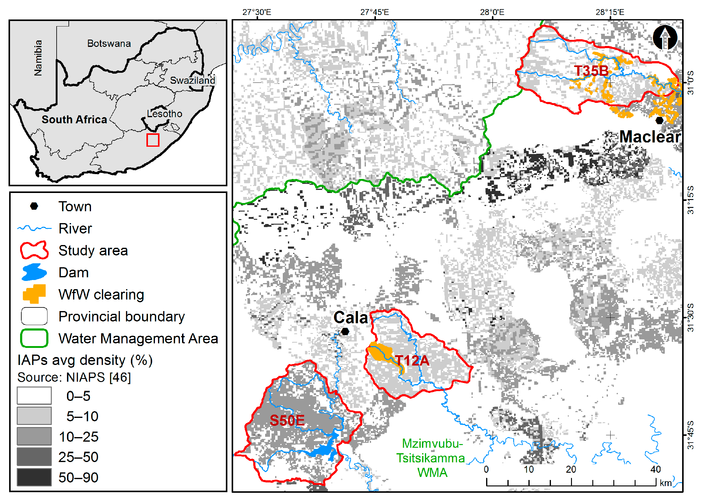
This paper describes the use of independent LC maps for change analysis in a grassland-dominated landscape in the Eastern Cape of South Africa to delineate LCC trajectories that are crucial to accurately quantify water and carbon fluxes. Invasion by woody plants is a driver of grassland transformation, which influences ecosystem services provided by rangelands, such as forage production, water supply, habitat, biodiversity, carbon sequestration and recreation [38]. Therefore, from a rangeland management perspective, understanding the LC trajectories relating to grass production would be important for local farmers [38]. In addition, the success of the Working for Water (WfW) programme [2], which uses labour-intensive methods to clear invasive woody plants while supporting job creation [3], can be evaluated. As IAPs are reported to have a high total incremental water use compared with indigenous vegetation [39], clearing could salvage a significant proportion of water to maintain other ecosystem services [40,41].
The objectives of the paper include: (1) the post-classification editing and accuracy assessment of the existing national LC product [32]; (2) deriving and validating a second LC map [42] to facilitate change analysis; (3) performing LCC analysis on these datasets; and (4) delineating important LCC trajectories.

2. Materials and Methods

2.1. Study Area

Three quaternary catchments (labelled T35B, T12A and S50E in Figure 1) situated in the Mzimvubu-Tsitsikamma Water Management Area (WMA) in the Eastern Cape of South Africa were selected for investigation. The vegetation of the study area is best described as grassland interspersed with thicket, formal plantations and IAPs [43]. Grassland is the second largest biome in South Africa comprising almost 29% of the total area [44], of which about 30% has been permanently modified [43]. The grasslands comprise not only grass species, but also bulbous perennials that reappear annually [45]. Invasion by woody plants has transformed the grassland, which influences rangeland production. Vegetation diversity and richness have also been degraded by poor farming practices, such as overgrazing, burning and wood felling. The soils comprise mostly deep clayey loams to rocky soils.
In this rural landscape, communal farming is practiced alongside a strong commercial livestock sector. Grazing and crop cultivation are noticeable as the main land use practices [47,48]. The area consists of three different land tenure units, namely former commercial farms and traditional and betterment villages, predominantly in T12A and S50E, and former Transkei rural areas [48,49]. Major users of water and carbon in this socio-ecological system are livestock and alien trees. The local district municipality (Chris Hani) and Working for Water (WfW) Alien Plant Clearing Programme have been clearing IAPs in these catchments for the past twelve years, with the primary motivation of water saving [50]. The location of WfW clearings digitized for the WfW programme [3] can be seen in Figure 1 within T12A and south of T35B [46].
S50E (31°45′ S 27°30′ E; 44,760 ha), the southernmost catchment, represents an area with high grazing potential under communal tenure of the local headman with an eight percent density of different IAP species [46]. Within the catchment lies the Ncora Dam supplied by the Tsomo River. In close proximity to the east of S50E lies T12A (31°30′ S 27°45′ E; 27,870 ha). Further north, catchment T35B (31° S 28°15′ E; 39,550 ha) represents commercial/freehold land with many different land usages, including forestry, mixed livestock and crop production.
Rainfall in the study area occurs predominantly in summer with the highest rainfall measured in January. Figure 2 illustrates the annual rainfall variation in the study area derived from Tropical Rainfall Measuring Mission (TRMM) satellite data [51,52] validated with complete weather station data from Cala and Maclear (see Figure 1) with the median of approximately 680 mm. Over the study period, rainfall varied between a low of ~450 mm per annum in 2003 and a high of almost 950 mm in 2006, a year of extreme rainfall in all of the catchments [53]. The rainfall for the two years selected for landscape comparison displays significantly different (p < 0.05) precipitation volumes, with 2000 being a relatively wet year with ~850 mm, in contrast to 2014, when the area received only ~600 mm.

2.2. Data Selection

Two time steps (T1 and T2) were selected for analysis. The first time step (T1) was selected to describe the landscape in 2000 and coincided with the date of the South African National Land Cover (NLC) dataset [32], which is commonly applied in studies requiring LC as input [54,55,56,57,58,59,60]. This LC map was classified from multi-temporal Landsat 7 Enhanced Thematic Mapper imagery using primarily conventional per-pixel classifiers based on 2000–2001 conditions [32] with a minimum mapping unit of 1–2 ha [60] and 45 classes [32]. The year 2000 also corresponds to the launch of the Moderate Resolution Imaging Spectroradiometer (MODIS) satellites (Terra and Aqua) providing science quality data with high temporal and spectral resolution and intermediate spatial resolution [61] used in other modelling and comparison studies in this project [38].
In the interest of comparing compatible classes between LC datasets T1 and T2, a revised LC legend comprising eight classes (Table 1) was developed for this study aggregating detailed classes [62,63] under a number of conceptually broader classes [64] to create a common LC scheme before comparison.
For this study, the conceptual class “cultivated and managed terrestrial, primarily vegetated areas” was divided into “cultivated” (cultivated lands (CLs)) and “managed” (forest plantations (FPs)) vegetation, while “natural and semi-natural terrestrial primarily vegetated areas” was separated into grassland and low shrubs (unimproved grassland (UG)) and wooded vegetation (forest indigenous, thicket bushlands (FITBs)) based on the original NLC legend (Table 1). Due to the low reported overall accuracy (65.8%) of the selected T1 dataset [32], it was systematically updated using the revised legend (Table 1) with aggregated LC classes, subsequently referred to as Edited National Land Cover (ENLC) 2000 for T1. Some tracts, labelled “degraded unimproved (natural) grassland”, were recognized as subsistence farming and re-allocated to “CLs”, while some parcels were re-allocated to “urban/built-up (UrBu)” after identification as rural villages. Accuracy assessment was performed on the edited dataset using stratified random sample points (10137) generated using ArcGIS 10.3 (Environmental Systems Research Institute (Esri), Redlands, CA, USA). Classes were assigned from aerial photography (dated July 2000: Chief Directorate: National Geospatial Information (CD: NGI)) using the eight-class LC legend (Table 1). In addition, a new LC dataset was generated through image processing to represent the second time step (T2) for 2014, 15 years later [42], corresponding to the collection of field data [38].

2.3. Image Processing

Various steps were taken to complete the image processing to generate the LC dataset for 2014 (T2). These included developing supplementary datasets, image pre-processing and image classification [42]. An object-oriented supervised approach using geographic object-based image analysis (GEOBIA) was selected for classification of Landsat 8 imagery in eCognition Developer (Trimble, Munich, Germany) [65]. To categorize object-features into respective classes, a rule-based decision tree classification with defining threshold conditions was implemented.
To inform the DT classification, various supplementary datasets were developed. Stratified random sample points were generated from the existing LC map (NLC 2000) and buffered by 30 m to capture LC areas. A new class was then assigned to the area from aerial photographs for 2014 according to the new eight-class LC legend (Table 1). Field data (in situ) collected during field visits in 2014 (less than 100 points) were also included in these training data. In excess of 5000 points were used per catchment, with more points selected for LC classes with greater geographical extent, e.g., UG. To delineate urban areas (UrBu), density estimation was performed on the Spot Building Count (ESKOM, South African Electricity Supply Commission SBC) [66] data. Digitized boundaries of cultivated land (for CLs) and forest plantations (FP) were rasterized, and slope was derived from a digital elevation model (SUDEM, Stellenbosch University digital elevation model) [67].
Two suitable cloud-free Landsat 8 images (scenes LC81690812014121LGN00 and LC81700822014160LGN00, dated 1 May 2014 and 9 June 2014, respectively) covering the spatial extent of the study area were downloaded for analysis. Images for the dryer winter season were selected to enhance the possibility of detecting greener IAPs within dry grasslands [10]. The Landsat scenes were atmospherically corrected by normalizing the solar radiance through conversion of spectral radiance to atmospheric reflectance. This was done in ATCOR 2 (ReSe Applications Schläpfer, Wil, Switzerland) [68] using the radiance conversion to top of atmosphere (ToA) reflectance model by converting digital numbers (DN) to radiance using the gain and bias values found in the metadata of each image file. The Landsat scenes had little or no cloud cover. Haze removal was done using the ToA reflectance correction method to eliminate the atmospheric effect that can cause image contamination and obscure ground features [68], followed by scene sharpening in PCI Geomatica (PCI Geomatics, Markham, Ontario, Canada) [69] to improve the spatial resolution of the multi-bands in order to separate interspersed land cover classes by extracting small feature objects [70].
Spectral and vegetation indices were prepared from the stacked Landsat dataset to improve the decision tree (DT) construction. These included the Normalized Difference Vegetation Index (NDVI), Enhanced Vegetation Index (EVI), Normalized Difference Water Index (NDWI), Soil Adjusted Vegetation Index (SAVI) and tasselled cap brightness. NDVI was selected to separate indigenous forest from grasslands. To address the limitations of NDVI that is affected by soil brightness [71] and saturates in high biomass areas [72,73], EVI was calculated, as it shows greater sensitivity to vegetation change and reduces atmospheric effects on vegetation index values [73]. NDWI was used to improve delineation of wetlands as a result of its sensitivity to changes in liquid water content of vegetation canopies [74]. SAVI [75] was computed as a corrective index on soil brightness for areas with low vegetation cover (<40%) and exposed soil surface. The brightness algorithm [76,77] was calculated to represent the reflectance intensity of bare rocks and soils among other features sharing similar spectral radiance.
Image pixels with relative homogeneity were clustered using the multi-resolution segmentation (MRS) algorithm [78,79]. MRS is an ascending area-merging technique where smaller objects are progressively merged into larger objects controlling the advancement in heterogeneity with three input parameters: scale, shape and compactness [70]. Shape and compactness were weighted at 0.1 and 0.5, respectively. Scale, referred to as the “window of perception” [80], is a unit-less parameter that regulates the size and homogeneity of image objects. Scale was set to two due to land cover heterogeneity in the study area. All layers were given equal importance in the segmentation settings, except near infrared and red bands, which received double weighting to increase their response signal to vegetation greenness. A bottom-up, region-growing segmentation approach was used to produce consistent results across the relatively large and heterogeneous study area. A minimum mapping unit of 1825 m2 (3 × 3 pan-sharpened pixels [21,27]) was selected to capture small fragmented LC classes.
A decision tree (DT) is defined as a classification procedure that recursively partitions a dataset into smaller subdivisions according to a decision framework defined by a tree structure [81]. Not only are DTs nonparametric and do not require assumptions regarding the distributions of the input data, but the classification structure is explicit and easy to interpret, making the method intuitive. Using training classes derived from aerial photographs with eight land cover classes (Table 1), a preliminary DT was generated in the classification and regression trees (CART) software [82] from which the final rule-set for the LC mapping was constructed [70]. The shadows class from the classified LC maps was incorporated into the surrounding vegetative cover class, validated by visual assessment from aerial photographs. The LC maps were combined into a single dataset referred to as Derived Land Cover (DLC) 2014 (T2).

2.4. Accuracy Assessment

Since accuracy measures estimated from a sample are subject to uncertainty [26,35,83], a more robust approach is to report the estimated error matrix in terms of the proportion of the area and the estimates of overall accuracy, user’s accuracy and producer’s accuracy based on the population [83] along with an associated confidence interval, providing a range of values for the reported parameter, which takes the uncertainty of the sample-based estimate into account. Accuracy assessment of both ENLC 2000 for T1 and DLC 2014 for T2 was performed by cross tabulation of the estimated area of observed reference classes vs. predicted classes. Stratified random sample points were generated per LC class using ArcGIS 10.3 (Esri, Redlands, CA, USA) and classes assigned from aerial photography of the same year. The estimated proportion of area for each cell of the error matrix was calculated and the error matrix of the estimated proportions constructed [26]. Accuracy measures calculated from this error matrix include the proportion correctly classified or overall accuracy, producer’s accuracy and user’s accuracy [84] with the 95% confidence interval computed from the standard error of the estimated area [35].

2.5. Change Analysis

The most commonly-used LCC detection method is the comparative approach, whereby categorical LC maps generated independently at different time steps are compared using a transition matrix to identify the most important transitions [83,85]. The basis for this method is an accurate LC map at each time step. Errors in these LC maps will be propagated to the change map, with expected error greater than in either of the maps from which it originated [11,31,85].
LCC analysis was performed by comparing the reference dataset ENLC 2000 from Time Step 1 (T1) to the classified dataset DLC 2014 from Time Step 2 (T2) in a transition matrix. Rows in the transition matrix represent the LC at T1, while columns represent LC at T2. From the transition matrix, net gain and loss per class can be calculated. The accuracy of the resulting LCC map was quantified from the accuracies of the individual LC maps at T1 and T2 by multiplying the individual accuracies for each classified map [31,33,37,85] since the pattern of error observed in the LCC map reflects the errors in the individual input classified maps and their interactions [16] if the classification errors are independent [31]. This is unlikely, as locations that were difficult to classify correctly at T1 would also be difficult to classify correctly at T2 even if different methodologies are used [84]. The probability of a particular class transition occurring can be calculated from the user’s accuracies for each LC map [33], which give the conditional probability that a pixel transitioned from the LC class in its row to the class in its column. Theoretical (D), upper (U), middle (M) and lower (L) bounds for estimates of change were calculated [33] from the user’s accuracy per LC class for each input map (T1 and T2) and reported in a transition matrix. Matrix D assumes the LC maps from T1 and T2 to be perfectly accurate, while matrix M assumes possible error in all pixels; matrix U considers error only in areas that correspond between T1 and T2, whereas matrix L considers error in places that differ between T1 and T2 and assumes no error in pixels that match [33]. The level of change was measured with 75% reliability (75% of the observed difference between the maps is real change) [31], calculated as a function of the accuracy of each input LC map, the eight classes mapped and the percentage change detected according to Figure 3 [31].

2.6. LCC Trajectories

Seven main flows or trajectories of aggregated LCC were identified [7,12] and are listed in Table 2 (highlighted with grey background). These trajectories include: (1) persistence, where no LCC has occurred; (2) intensification, which represents the transition of a lower intensity to a higher intensity usage; (3) afforestation representing the planting of trees; (4) deforestation, which involves the clearance of trees; (5) extensification where higher intensity usage is converted to a lower intensity usage; (6) natural dynamics to represent seasonal conversions; and (7) exceptionality associated with potential map errors. In the context of this study, these seven categories were subdivided to account for specific changes in this landscape (Table 2). As part of persistence (P), label Pf (FITB persistence) indicates areas where woody vegetation (including indigenous forest and IAPs) has persisted, while label Pu (Urban persistence) describes areas where settlements have persisted over time. Of particular importance are areas where forests (indigenous or alien) and other woody areas have disappeared or been removed (reclamation, deforestation) or another LC has potentially been replaced by IAPs (FITB intensification). Due to the resolution of the satellite imagery used in the generation of the LC classes, it was not possible to determine change in the intensity of agricultural activities, but conversion to agricultural practices can be identified (agricultural intensification). Exceptionality indicates where an improbable conversion occurs, such as to wetland, which may be used to identify classification errors.
The use of an LC conversion label not only allows a thematic representation of the spatial distribution of change [13], but also provides information about the processes (flows) in the landscape [7] that can be represented on a map to simplify the evaluation of LCC. From the intersection of the two LC layers, a square transition matrix was created where rows show the classes from 2000 (T1), columns show the same classes from 2014 (T2) and the table entry indicates the size of the class (in pixels or percentage of study area) at the intersection created by the overlay of the successive LC maps. An LC conversion label from Table 2 was assigned to each intersection representing the process flow depicted in Table 3. This conceptual schema of using LC conversion labels [13] for change analysis was developed to describe patterns and trajectories both qualitatively and quantitatively. The area for each LC conversion label was calculated and expressed as a percentage of the total area of each of the catchments.

3. Results

3.1. Accuracy Assessment of Datasets for T1 and T2

Table 4 presents the accuracy assessment for the LC map ENLC 2000 for Time Step 1 (T1) obtained after updating the existing National Land Cover (NLC) dataset [32] based on sample counts. Rows represent map categories, while reference categories are given in the columns. Table 4 also reports the area for each map category and the percent of the study area to the nearest integer, where a zero means a positive number less than one half and a dash means that no pixels were observed. Table S1 in the Supplementary Material provides the detail at the catchment level. Table 5 illustrates the accuracy of the T1 dataset based on Table 4 data expressed as the estimated percent of the study area (the population). Accuracy measures, overall accuracy (OA), user’s accuracy (UA) and producer’s accuracy (PA) are presented with a 95% confidence interval [26].
Based on the sample counts (Table 4) and estimate of the population (Table 5), the overall accuracy of the T1 dataset (ENLC 2000) is 84% with a 95% confidence interval of 1% based on the calculated standard error. This is almost 20% more than the uncorrected NLC 2000 dataset [32]. A summary of the accuracy assessment performed on the DLC 2014 dataset, which was derived through classification of Landsat 8 imagery for time step T2, based on sample counts, is presented in Table 6. Catchment level results are demonstrated in Table S2. The descriptions for abbreviations used as column headings can be found in Table 1. The rows represent the map categories, while columns represent reference categories. The areas computed from the map categories, as well as the percent of total area are also shown in Table 6. Similar to Table 5, Table 7 illustrates the accuracy of the T2 dataset based on Table 6 data expressed as the estimated proportion of area (the population) reported as the percent, where a zero means a positive number less than one half and a dash means that no pixels were observed.
The producer’s accuracy is a measure of how well a certain area has been classified and indicates the probability of a reference sample being correctly classified (not omitted) [84]. Wetlands (Wl) were poorly predicted with a low producer’s accuracy of 36% based on sample counts, which means that more than sixty percent of the reference samples were omitted from the classification (error of omission). The effect of ignoring the population matrix is clearly illustrated, as the producer’s accuracy calculated from the area proportion is as low as 10% ± 3%, reflecting the uncertainty in the classification. Based on the reference classification, the stratified area for LC class Wl can be calculated as 3981 ± 492 ha, more than seven-times the mapped area. An error-adjusted estimate of the area covered by Wl (±95% confidence interval) confirms the need to adjust the map area obtained from pixel counting to account for the large omission error. FITBs and bare rock and soil (BRS) also showed low producer’s accuracies. The user’s accuracy indicates for a given class how many of the pixels on the map are actually classified correctly and can be computed directly from the sample counts [26]. The FITB class, representing natural wooded areas, including IAPs, produced in the classification showed a user’s accuracy of greater than 90%, but poorer producer’s accuracy of only 55% ± 2%. The overall accuracy based on reference point data, computed as correctly classified divided by the total, ranged between 83% (T35B) and almost 90% (S50E) (Table S2) using sample points (Table 6), but did not differ much when using the proportion of estimated area (Table 7). The overall accuracy for T35B was 83% ± 1% and for S50E slightly lower at 87% ± 1%. The overall accuracy for the study area was calculated as 85% ± 1% (Table 7).

3.2. Land Cover Change: ENLC 2000 vs. DLC 2014

From the LC maps at the two-time steps, a post-classification comparison was made of the overlaid LC maps for 2000 (T1) and 2014 (T2) using a transition matrix. Table 8 shows the transition from one LC class to another as a percent of the study area. Four values are reported per LCC combination: the left entries in the cells represent D, assuming each input LC map to be completely accurate; the upper right entries are the upper bound (U) where error exists in corresponding areas; the middle right entries (M) assume possible error in all pixels; and the lower right entries (L) assume no error in matching pixels. Descriptions of class labels can be found in Table 1. The rows represent the T1 (2000) LC classes, while the T2 (2014) LC classes are found in the columns. The diagonal entries (light grey in Table 8) indicate the persistence of LC classes, while the off-diagonal entries indicate a change from one LC class to a different class. The Total T1 column shows the LC totals at 2000, and the Total T2 row shows the LC totals at 2014 expressed as a percent of the total study area. The column on the right (Loss T1) indicates loss by LC class, and the row at the bottom (Gain T2) indicates gain by LC class. The total change as a proportion of the total study area is given in the entry in the bottom row of column Loss T1. The columns UA and PA reflect the product of the user’s and producer’s accuracy for each individual LC map (T1 and T2) providing a theoretical accuracy for the transition per class.
Grassland (UG) still dominates the study area in 2014 with 68% of the total area still classified as such when measuring change using the T1 and T2 maps without considering error (accuracy 84% × 85% = 71%). Though UG has the highest theoretical producer’s accuracy of 94%, the remaining UG could be as low as 58% when considering possible error in all pixels (matrix M). Net losses were noted for UG and FP, with gains in UrBu. No change was calculated for Wb. For classes FITBs, BRS and CLs, the net gain or loss was dependent on the method for calculating land change (matrix D, M, U or L). CLs showed a net gain of 1% when no error is considered, but up to 2% loss when possible error in all pixels is considered (M). The low PA for CLs of 63% confirms large differences between map and ground conditions. In addition, the theoretical accuracy of the resulting LCC maps, computed as the product of the overall accuracies of the individual LC maps at T1 and T2 [11,31,85], ranged between a low 67% for T35B to 76% for T12A (Table S3). This leaves a hypothetical error in landscape transition of up to 30% based on error propagation from contributing LC maps. The total change, computed from loss at T1 and gain at T2, varies between 18% and 42% calculated from the lower (L) and upper (U) bounds of change (lower right cell, Table 8) with 19% computed from the overlay of the T1 and T2 maps.
Assuming that map errors are independent and changes are mapped correctly within the area of overlap, the accurately-mapped difference due to change (c), as well as those changes that are hidden can be calculated [31]. Areas with no change (persistence) can also be identified. Table 9 assesses the likely differences due to change and those due to error [31]. Where the LCC map reflects the true situation (change or persistence), the cell text in Table 9 is shown in bold; true change hidden by errors is given in italic text; and where the map records a difference (change or error), the cells are shaded.
With the change of 19% calculated from Table 8 and the levels of accuracy estimated for T1 (Table 5) and T2 (Table 7), there would only be a 59% agreement between the two LC maps, and 41% of the combined map area would record differences. Of the 41% difference, ~18% would be real change, and ~23% would have arisen through errors. With a change of 40% (matrix M from Table 8), there would only be an agreement of 45% between the maps and 55% difference. Though there is substantial over-estimation of changed areas in both scenarios, 96% of all change could be mapped.

3.3. Land Cover Conversion Dynamics

Using the conceptual schema of LC conversion labels (Table 2 and Table 3) in analysing the change matrix statistics, quantitative analysis was performed for the landscape transition between the two time periods. Transitions from and to LC classes BRS and Wl were not characterized according to Table 3, but were added to LC conversion label E (exceptionality) due to the low user’s and producer’s accuracy for these two classes. Table 10 summarizes the conversion dynamics by area and percent of catchment area to the nearest integer, where zero indicates a positive number less than one half, and a dash means no transitions were observed. Figure 4 provides the spatial distribution of these LC conversions using the indicator-based approach (LC labels) to visualize change trajectories.
Land use patterns in all three catchments are characterized by persistence (Figure 4 LC labels P, Pu and Pf) with more than 70% of the total area showing no change. Conversions between classes represent small fragmented areas of less than six percent within the catchments. Intensification of woody vegetation where class FITBs have substituted previous LC averaged at four percent, while reclamation (Re) to grassland was four percent over all three catchments. Transitions from plantation, labelled deforestation (D), covered one percent of the study area extent, while afforestation (R) mostly affected T35B. Degradation (De) linked to conversion to bare soil was not represented due to the low accuracy of LC class BRS. Exceptionality (E), indicating possible classification errors and LC classes with high uncertainty (BRS and Wl) represented one percent of land transformation. The highest exceptional trajectories were found in catchment T35B, caused by the high presence of Wl.

4. Discussion

This paper describes the challenges encountered while performing change analysis to determine landscape conversion dynamics between two time steps represented by two datasets derived using different methods. The original input dataset proposed for Time Step 1 (T1) proved unsatisfactory based on overall accuracy and was subsequently improved using manual methods. The T1 dataset was derived from a national level dataset frequently used for studies that require LC as input, such as the quantification of runoff and infiltration for a particular LC unit [58]. Users often do not consider the low reported accuracy. As this dataset coincides with the availability of high temporal resolution MODIS data, it is frequently used as a starting point for area-based spatial analysis studies.
The dataset for Time Step 2 (T2) is the output of the object-based classification of Landsat 8 data. The OBIA approach was able to deal with the problem of the salt-and-pepper effect, common in classification outcomes using traditional per-pixel approaches [21], while the rule-based expert system provided robust LC classifications for highly fragmented catchment landscapes and precision in delineating boundaries of the various vegetation types despite the coarser Landsat 8 resolution [21,86]. The overall accuracy for this LC dataset (T2) using single-date imagery was deemed acceptable based on the overall accuracy value of greater than 85% ± 1% when compared to reference points (Table 7) expressed as the estimated percent of area (the population). Sufficient ground truth data are required for definite mapping of alien plants and other cover classes.
As LC classification is fraught with uncertainty, it is important to accurately report on the uncertainty inherent in data created through spatial modelling [26,35], which starts with an effective sampling design of ground truth data [35]. Estimates of overall accuracy, user’s accuracy and producer’s accuracy based on the population [83] can be reported. A confidence interval can be computed, to describe the uncertainty of the sample-based estimates. In addition, the construction of a meaningful LC legend through categorical aggregation in a manner that gives insights concerning categorical change over time [62] that can accommodate these wooded classes must be investigated. However, it must be noted that category aggregation may decrease the error in the individual LC maps, as well as the difference between LC maps at T1 and T2 [87].
LCC detection was performed using a transition matrix to compare the categorical LC maps from the two time steps. The method (D) assumes that the probability of error in the two independently-classified maps (T1 and T2) is randomly distributed, which is unlikely, as error is affected by autocorrelation [37]. Upper (U), middle (M) and lower bounds of LCC were also reported. Method U assumes that error only exists where LC maps match; therefore, more error is associated with higher estimated change, up to 42% in this study area. Simulated errors cause a shift of values from the diagonal to the off-diagonal entries of the transition matrix [33]. In contrast, method L considers that error exists only in areas of change, therefore more error with less estimated change [33]. As some classes are easier to classify than others, and such regions are frequently clustered [84]; the error may exhibit spatial autocorrelation. This would cause large homogenous classes, such as UG, to exhibit small errors compared to fragmented small classes, such as woody outcrops with many edges around small patches. This is clear from the high producer’s accuracy for the UG class (Table 5 and Table 7) and low producer’s accuracy for FITBs. Error may also be temporally autocorrelated, such as classes on flat slopes that persist over time, which may be easier to classify [37]. Future studies should therefore consider investigating the spatial and temporal correlation of error within the input LC maps prior to LCC analysis, to reduce errorpropagation [34,88]. The accuracy for the LCC map was derived from the overall accuracies of the individual LC maps (84% and 85%, respectively) resulting in a low overall accuracy of 71%. From 
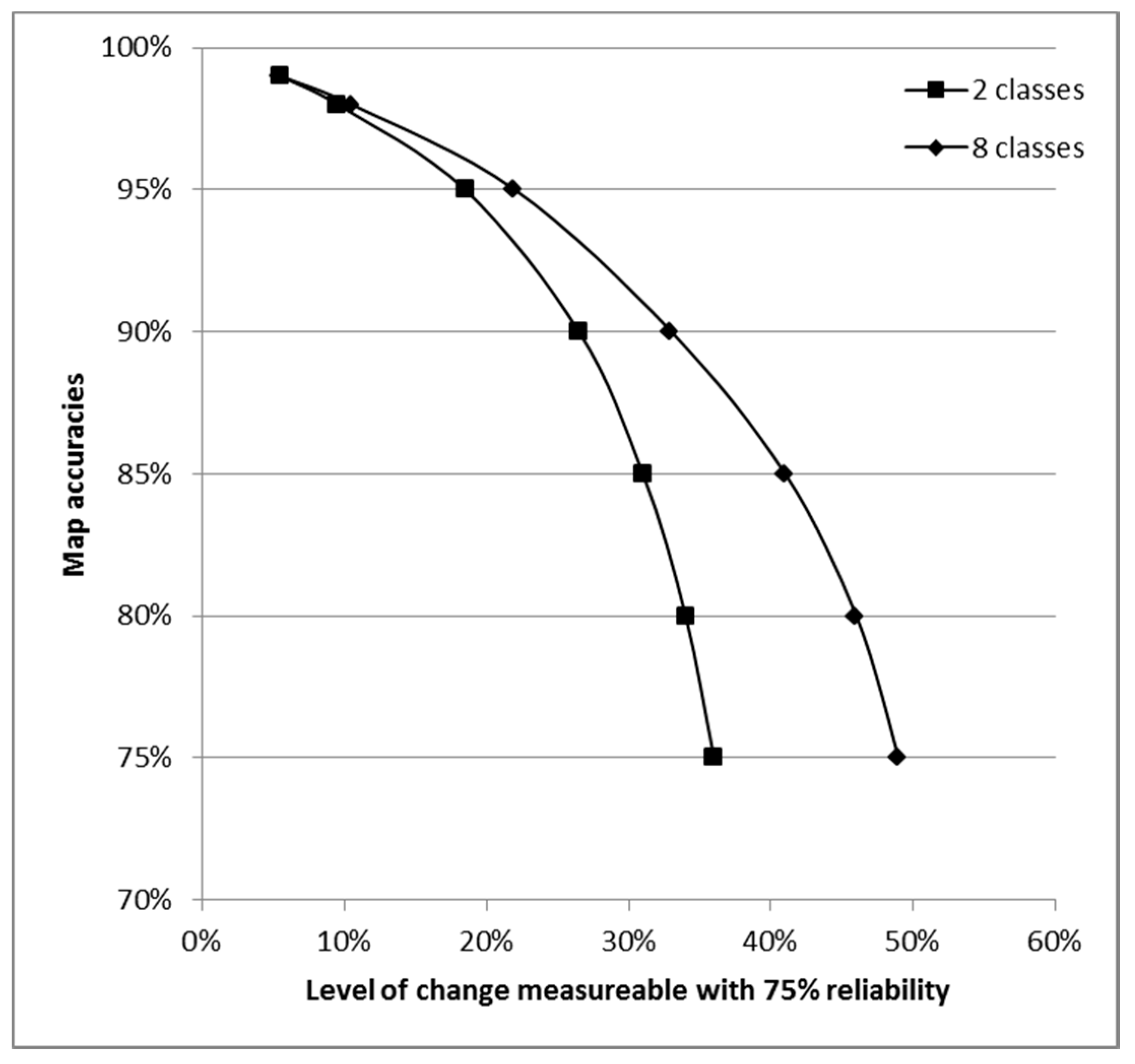
Figure 3, the level of change that can be recorded with 75% reliability on maps with 2, 3, 10 and 30 classes with a particular accuracy can be determined [31]. To map a change such as 19% (Table 8), input LC maps would need to be about 96% accurate, assuming 75% reliability. Should greater reliability be required, map accuracies need to approximate 99% [89], which has become the operational requirement. Theoretical accuracy of greater than 70% was achieved for the LCC maps for the southern catchments (T12A and S50E) with T35B showing greater uncertainty at 67%. Individual classes BRS and Wl displayed low producer’s accuracies, which caused conversion trajectories involving these classes to be flagged as exceptionality and excluded from the trajectory analysis.
This study used a framework for change analysis [7,13,85] based on change trajectories derived from LC labels (Table 3) categorizing combinations of LCC into seven main flows or trajectories. When this framework was applied to the LCC maps, the persistence of LC classes (>70% from 
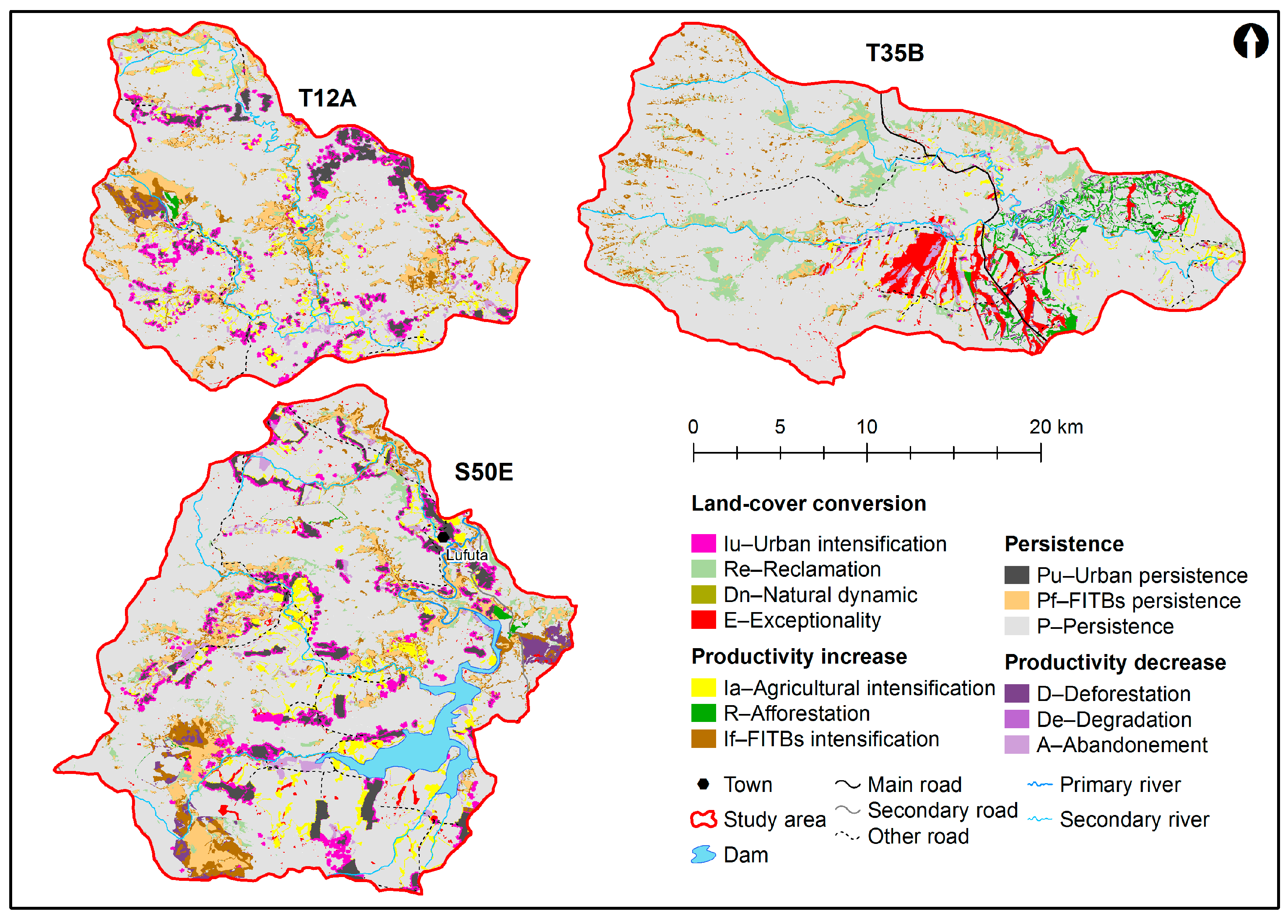
Table 10) was noted with grassland remaining the majority cover in the three catchments. Both urban persistence (Pu) and FITB persistence (Pf) are clearly visible in catchments T12A and S50E (Figure 4) with the expansion of urban areas (Iu, urban intensification) in these two southern catchments predominantly at the expense of grassland (UG) and agriculture (CLs), demonstrating the natural development of urban areas. Urban intensification is also highest in these catchments where subsistence farming is practiced. This apparent intensification may possibly be attributed to the T1 dataset classification strategy, which focused on identifying formal townships and failed to delineate traditional villages practicing subsistence farming, as encountered in these areas. Accordingly, agricultural activities intensified (Ia) by four percent in S50E, attributed to conversion from grassland (UG) when no error is considered, but up to 2% loss when possible error in all pixels is considered (M), associated with low user’s and producer’s accuracies for CLs in LC classification.
Considering that the class FITBs contains indigenous forest, thicket, bushland, bush clumps, high fynbos and alien plants that are spectrally similar and could not be separated using Landsat imagery, it is not surprising that T12A, with persistent remnants of indigenous forest, has the highest percentage of the class FITB persistence (Pf). The high persistence of FITBs (Pf) in S50E is likely attributed to the presence of Pinus spp. [43] on the southwest of the catchment. Interestingly, despite T12A being a focus target for Working for Water (WfW) with the aim of eradicating alien trees in these catchments, there is still a prominent presence. In both the T1 and T2 datasets, the low producer’s accuracy for FITBs highlights the uncertainty associated with this transition. In order to provide a better distinction between different wooded classes, higher spatial resolution data need to be considered to distinguish between spectrally-homogenous vegetation types [72].
Since scientists want to identify the dominant signals of land change, the varying dynamics between the three catchments must be noted. Accounting for approximately four percent of the study extent, agricultural intensification (Ia) and afforestation (R) can be regarded as an increase in the productivity of the landscape, with land use intensification associated with a productivity-driven landscape. Conversely, the persistence and intensification of FITBs (Pf + If) may be regarded as a degradation gradient existing in the landscape, when IAPs included in the FITBs class affect biodiversity and ecosystem services. T12A and S50E have similar trajectories of this degradation gradients (Pf + If), which may reflect real change or be an artefact of the classification and LCC detection. After persistence, this is the strongest conversion trajectory within these two catchments. It can be postulated that the FITB persistence and intensification noticeable in T12A and S50E may be attributed to IAPs, known to affect grassland veld types [45].
The context of reclamation (Re) in this study designates the potential extent of anthropogenic rehabilitation, where areas classified as FITBs (invaded by IAPs and other woody vegetation) have been replaced with grassland and bare rocks. Despite reported WfW activity, reclamation (Re) in T12A and S50E was less than three percent. In T35B, six percent of FITBs have been returned to grassland, an area of almost 2400 ha. This however may be an artefact associated with the low accuracy of the LCC map for T35B (Table S3). Spatial analyses of the locational factors, which may be driving the LCC trajectories [36,89,90,91], are envisaged for future research.

5. Conclusions

This paper has described the use of independent LC maps for change analysis in a grassland-dominated landscape for three catchments in the Eastern Cape of South Africa. Land cover maps were derived from existing national LC dataset data (2000-T1) and through object-based image analysis (2014-T2) of Landsat 8 imagery. A revised LC legend comprising eight classes was developed aggregating detailed classes under a number of conceptually broader classes to create a common LC scheme in the interest of comparing compatible classes between LC datasets T1 and T2.
Accuracy assessment of the independently-created LC maps revealed the overall accuracies to be 83.7% and 85.4% for T1 and T2, respectively. The theoretical accuracy of the resulting LCC maps, ranged between a low 67% for T35B to 72% for S50E and 76% for T12A (Table S3) with a hypothetical error in landscape transition of up to 30% based on error propagation from contributing LC maps. Land use patterns in all three catchments are characterized by persistence with more than 70% of the total area showing no change. However, despite the high accuracies for the independently-mapped LC at T1 and T2, 37% of the combined map area would record differences of which ~19% would be real change and ~19% would have arisen through errors. Through substantial over-estimation of areas’ change, 96% of all change could be mapped.
The LCC analysis has revealed an increase of agricultural intensification, urbanization and infrastructural development across the three catchments over the 15-year period. LC class FITBs in the guise of natural vegetation or alien plants have persisted and intensified chiefly at the periphery of river channels, as well as around agricultural areas and human inhabited regions. While some LC classes, such as grassland and water bodies, have maintained approximate states of persistence, land degradation resulting from land use intensification and FITBs (possibly IAPs) infestations has been identified.
LC classification is fraught with uncertainty; thus, accurate reporting on this inherent uncertainty is needed if water and carbon fluxes are to be properly understood and quantified, especially where future scenarios may be considered. In this study area, it was revealed that at the current level of change, for 75% reliability of results, an overall accuracy of LC maps of 96% would be required. Should higher reliability of change results be required for operational purposes, accuracies of 99% for each independently mapped LC dataset would be required. Achieving these levels of accuracies at Landsat resolution is unlikely, and thus, some uncertainty in both the classification results and the change results must be accepted.
Landscape units associated with clearly identified persistent or degradation trajectories can be used in future studies to characterize water use and carbon fluxes for sustained landscape health from remote sensing products allowing models of ecosystem stress to be developed. The challenge remains to determine significant signals in the landscape that are not artefacts of the underlying input data, different classification schemes and aggregation methods, the experience of classifiers or the scale of analysis. Through systematic analysis of changes and accurate reporting of uncertainty, this can be addressed to produce output that authentically reflects the landscape dynamics in order to accurately quantify the effect of landscape transitions on the ecosystems services in the catchments.

Supplementary Materials

The following are available online at www.mdpi.com/2076-3263/7/1/7/s1: Table S1: Accuracy assessment of the ENLC 2000 (T1) per catchment; Table S2: Accuracy assessment of DLC 2014 (T2) per catchment; Table S3: Theoretical accuracy of LCC analysis.

Acknowledgments

This work was supported by the South African Water Research Commission Project K5/2400/4. Data processing support was provided by the Centre for Geographical Analysis, Stellenbosch University.

Author Contributions

Sukhmani Mantel and Anthony Palmer conceived of the project. Zahn Münch designed the experiments. Perpetua I. Okoye performed the land cover classification. Zahn Münch and Perpetua I. Okoye analysed the data and wrote the paper. Zahn Münch and Lesley Gibson provided editorial support and major revisions.

Conflicts of Interest

The authors declare no conflict of interest.

References

  1. Le Maître, D.C.; Gush, M.B.; Dzikiti, S. Impacts of invading alien plant species on water flows at stand and catchment scales. AoB Plants 2015, 7, plv043. [Google Scholar] [CrossRef] [PubMed]
  2. Turpie, J.K.; Marais, C.; Blignaut, J.N. The working for water programme: Evolution of a payments for ecosystem services mechanism that addresses both poverty and ecosystem service delivery in South Africa. Ecol. Econ. 2008, 65, 788–798. [Google Scholar] [CrossRef]
  3. Driver, A.; Sink, K.J.; Nel, J.N.; Holness, S.; Van Niekerk, L.; Daniels, F.; Jonas, Z.; Majiedt, P.A.; Harris, L.; Maze, K. National Biodiversity Assessment 2011: An assessment of South Africa’s biodiversity and ecosystems. Synthesis Report. South African National Biodiversity Institute and Department of Environmental Affairs: Pretoria, 2012; p. 180. Available online: http://catalog.ipbes.net/system/assessment/195/references/files/570/original/NBA_2011_Synthesis_Report_%28low_resolution%29.pdf?1364385861 (accessed on 11 July 2016).
  4. Lambin, E.; Geist, H. Causes of Land Use and Land Cover Change. 2007. Available online: http://www.eoearth.org/view/article/51cbed2f7896bb431f6905af (accessed on 4 April 2014).
  5. Diaz, S.; Fargione, J.; Chapin, F.S., III; Tilman, D. Biodiversity loss threatens human well-being. PLoS Biol. 2006, 4, e277. [Google Scholar] [CrossRef] [PubMed]
  6. Brown, T.C.; Bergstrom, J.C.; Loomis, J.B. Defining, valuing, and providing ecosystem goods and services. Nat. Resour. 2007, 47, 329–376. [Google Scholar]
  7. Feranec, J.; Jaffrain, G.; Soukup, T.; Hazeu, G. Determining changes and flows in European landscapes 1990–2000 using CORINE land cover data. Appl. Geogr. 2010, 30, 19–35. [Google Scholar] [CrossRef]
  8. Bastian, O.; Krönert, R.; Lipsky, Z. Landscape diagnosis on different space and time scales—A challenge for landscape planning. Landsc. Ecol. 2006, 21, 359–374. [Google Scholar] [CrossRef]
  9. Reyers, B.; O’Farrell, P.J.; Cowling, R.M.; Egoh, B.N.; Le Maitre, D.C.; Vlok, J.H.J. Ecosystem services, land-cover change, and stakeholders: Finding a sustainable foothold for a semiarid biodiversity hotspot. Ecol. Soc. 2009, 14, 38. [Google Scholar] [CrossRef]
  10. Huang, C.Y.; Asner, G.P. Applications of remote sensing to alien invasive plant studies. Sensors 2009, 9, 4869–4889. [Google Scholar] [CrossRef] [PubMed]
  11. Aldwaik, S.Z.; Pontius, R.G., Jr. Map errors that could account for deviations from a uniform intensity of land change. Int. J. Geogr. Inf. Sci. 2013, 27, 1717–1739. [Google Scholar] [CrossRef]
  12. Stott, A.; Haines-Young, R. Linking land cover, intensity of use and botanical diversity in an accounting framework in the UK. In Environmental Accounting in Theory and Practice; Uno, K., Bartelmus, P., Eds.; Kluwer: Dordrecht, The Netherlands, 1998; pp. 245–260. [Google Scholar]
  13. Benini, L.; Bandini, V.; Marazza, D.; Contin, A. Assessment of land use changes through an indicator-based approach: A case study from the Lamone river basin in Northern Italy. Ecol. Ind. 2010, 10, 4–14. [Google Scholar] [CrossRef]
  14. Nagendra, H.; Munroe, D.K.; Southworth, J. From pattern to process: Landscape fragmentation and the analysis of land use/land cover change. Agric. Ecosyst. Environ. 2004, 101, 111–115. [Google Scholar] [CrossRef]
  15. Lambin, E.F.; Geist, H.J.; Lepers, E. Dynamics of land use and land cover change in tropical regions. Annu. Rev. Environ. Resour. 2003, 28, 205–241. [Google Scholar] [CrossRef]
  16. Burnicki, A.C. Spatio-temporal errors in land–cover change analysis: Implications for accuracy assessment. Int. J. Remote Sens. 2011, 32, 7487–7512. [Google Scholar] [CrossRef]
  17. Cowling, R.M.; Egoh, B.; Knight, A.T. An operational model for mainstreaming ecosystem services for implementation. PNAS 2008, 105, 9483–9488. [Google Scholar] [CrossRef] [PubMed]
  18. Szantoi, Z.; Brink, A.; Buchanan, G.; Bastin, L.; Lupi, A.; Simonetti, D.; Mayaux, P.; Peedell, S.; Davy, J. A Simple Remote Sensing Based Information System for Monitoring Sites of Conservation Importance. Remote Sens. Ecol. Conserv. 2016, 2, 16–24. [Google Scholar] [CrossRef]
  19. Schoeman, F.; Newby, T.S.; Thompson, M.W.; Van den Berg, E.C. South African National Land-Cover Change Map. SA J. Geomat. 2013, 2, 94–105. [Google Scholar]
  20. Bodart, C.; Brink, A.B.; Donnay, F.; Lupi, A.; Mayaux, P.; Achard, F. Continental estimates of forest cover and forest cover changes in the dry ecosystems of Africa between 1990 and 2000. J. Biogeogr. 2013, 40, 1036–1047. [Google Scholar] [CrossRef] [PubMed]
  21. Blaschke, T. Object based image analysis for remote sensing. ISPRS J. Photogramm. Remote Sens. 2010, 65, 2–16. [Google Scholar] [CrossRef]
  22. Campbell, J.B.; Wynne, R.H. Introduction to Remote Sensing, 5th ed.; The Guilford Press: New York, NY, USA, 2011. [Google Scholar]
  23. Linke, J.; McDermid, G.J.; Pape, A.D.; McLane, A.J.; Laskin, D.N.; Hall-Beyer, M.; Franklin, S.E. The influence of patch-delineation mismatches on multi-temporal landscape pattern analysis. Landsc. Ecol. 2011, 24, 157–170. [Google Scholar] [CrossRef]
  24. Tseng, M.H.; Chen, S.J.; Hwang, G.H.; Shen, M.Y. A genetic algorithm rule-based approach for land cover classification. ISPRS J. Photogramm. Remote Sens. 2008, 63, 202–212. [Google Scholar] [CrossRef]
  25. Pal, M.; Mather, P.M. An assessment of the effectiveness of decision tree methods for land cover classification. Remote Sens. Environ. 2003, 86, 554–565. [Google Scholar] [CrossRef]
  26. Olofsson, P.; Foody, G.M.; Stehman, S.V.; Woodcock, C.E. Making better use of accuracy data in land change studies: Estimating accuracy and area and quantifying uncertainty using stratified estimation. Remote Sens. Environ. 2013, 129, 122–131. [Google Scholar] [CrossRef]
  27. MacLean, M.G.; Congalton, R.G. Map accuracy assessment issues when using an object-oriented approach. In Proceedings of the American Society for Photogrammetry and Remote Sensing 2012 Annual Conference, Baltimore, MD, USA, 16–19 March 2012; pp. 1–5.
  28. Congalton, R.G.; Green, K. Assessing the Accuracy of Remotely Sensed Data: Principles and Practices, 2nd ed.; CRC Press: Boca Raton, FL, USA, 2009; p. 208. [Google Scholar]
  29. Foody, G.M. Status of land cover classification accuracy assessment. Remote Sens. Environ. 2002, 80, 185–201. [Google Scholar] [CrossRef]
  30. Homer, C.; Dewitz, J.; Yang, L.; Jin, S.; Danielson, P.; Xian, G.; Coulston, J.; Herold, N.; Wickham, J.; Megown, K. Completion of the 2011 National Land Cover Database for the Conterminous United States—Representing a Decade of Land Cover Change Information. Photogramm. Eng. Remote Sens. 2015, 81, 346–354. [Google Scholar]
  31. Fuller, R.M.; Smith, G.M.; Devereux, B.J. The characterisation and measurement of land cover change through remote sensing: Problems in operational applications? Int. J. Appl. Earth Obs. 2003, 4, 243–253. [Google Scholar] [CrossRef]
  32. Van den Berg, E.C.; Plarre, C.; Van den Berg, H.M.; Thompson, M.W. The South African National Land Cover 2000; Unpublished Report No. GW/A/2008/86; Agricultural Research Council-Institute for Soil, Climate and Water: Pretoria, South Africa, 2008. [Google Scholar]
  33. Pontius, R.G., Jr.; Li, X. Land transition estimates from erroneous maps. J. Land Use Sci. 2010, 5, 31–44. [Google Scholar] [CrossRef]
  34. Burnicki, A.C.; Brown, D.G.; Goovaerts, P. Simulating error propagation in land-cover change analysis: The implications of temporal dependence. Comput. Environ. Urban 2007, 31, 282–302. [Google Scholar] [CrossRef]
  35. Olofsson, P.; Foody, G.M.; Herold, M.; Stehman, S.V.; Woodcock, C.E.; Wulder, M.A. Good practices for estimating area and assessing accuracy of land change. Remote Sens. Environ. 2014, 148, 42–57. [Google Scholar] [CrossRef]
  36. Malek, Ž.; Scolobig, A.; Schröter, D. Understanding land cover changes in the Italian Alps and Romanian Carpathians combining remote sensing and stakeholder interviews. Land 2014, 3, 52–73. [Google Scholar] [CrossRef]
  37. Pontius, R.G., Jr.; Lippitt, C.D. Can error explain map differences over time? Cartogr. Geogr. Inf. Sci. 2006, 33, 159–171. [Google Scholar] [CrossRef]
  38. Gwate, O.; Mantel, S.K.; Finca, A.; Gibson, L.A.; Munch, Z.; Palmer, A.R. Exploring the invasion of rangelands by Acacia mearnsii (black wattle): Biophysical characteristics and management implications. Afr. J. Range Forage Sci. 2016, 33, 265–273. [Google Scholar] [CrossRef]
  39. Clulow, A.D.; Everson, C.S.; Gush, M.B. The Long-Term Impact of Acacia Mearnsii Trees on Evapotranspiration, Streamflow and Groundwater Resources; WRC Report No. TT505/11; Water Research Commission: Pretoria, South Africa, 2011. [Google Scholar]
  40. Van Wilgen, B.W.; Reyers, B.; Le Maitre, D.C.; Richardson, D.M.; Schonegevel, L. A biome-scale assessment of the impact of invasive alien plants on ecosystem services in South Africa. J. Environ. Manag. 2008, 89, 336–349. [Google Scholar] [CrossRef] [PubMed]
  41. Meijninger, W.M.L.; Jarmain, C. Satellite-based annual evaporation estimates of invasive alien plant species and native vegetation in South Africa. Water SA 2014, 40, 95–108. [Google Scholar] [CrossRef]
  42. Okoye, P.I. Grassland Rehabilitation after Alien Invasive Tree Eradication: Landscape Degradation and Sustainability in Rural Eastern Cape. Master’s Thesis, Stellenbosch University, Stellenbosch, South Africa, 2016. [Google Scholar]
  43. Mucina, L.; Rutherford, M.C. The Vegetation Map of South Africa, Lesotho and Swaziland. SANBI, Pretoria. 2006. Available online: http://www.sanbi.org/products/publications/stelitzia.htm (accessed on 28 July 2015).
  44. Van Wilgen, B.W.; Forsyth, G.G.; Le Maitre, D.C.; Wannenburgh, A.; Kotzé, J.D.F.; Van den Berg, E.; Henderson, L. An assessment of the effectiveness of a large, national-scale invasive alien plant control strategy in South Africa. Biol. Conserv. 2012, 148, 28–38. [Google Scholar] [CrossRef]
  45. Carbutt, C.; Tau, M.; Stephens, A.; Escott, B. The conservation status of temperate grasslands in southern Africa. Grassroots 2011, 11, 17–23. [Google Scholar]
  46. Kotzé, J.D.F.; Beukes, B.H.; Van den Berg, E.C.; Newby, T.S. National Invasive Alien Plant Survey; Report Number: GW/A/2010/21; Agricultural Research Council: Institute for Soil, Climate and Water: Pretoria, South Africa, 2010. [Google Scholar]
  47. Water Research Commission (WRC). Vulnerability, Adaptation to and Coping with Drought: The Case of Commercial and Subsistence Rainfed Farming in the Eastern Cape. Deliverable 1: Description and Demarcation of Study Area. WRC Project K4/2280. University of Free State, 2013. Available online: http://dimtecrisk.ufs.ac.za/wrc_ec/study_area/WRC_2280_study_area.htm (accessed on 25 July 2016).
  48. Kakembo, V. Trends in vegetation degradation in relation to land tenure, rainfall, and population changes in Peddie District, Eastern Cape, South Africa. Environ. Manag. 2001, 28, 39–46. [Google Scholar] [CrossRef] [Green Version]
  49. Wotshela, L. Land redistribution politics in the Eastern Cape midlands: The case of the Lukhanji municipality, 1995–2006. Kronos 2009, 35, 142–159. [Google Scholar]
  50. Dye, P.J.; Jarmain, C.; Le Maître, D.C.; Everson, C.S.; Gush, M.B.; Clulow, A. Modelling Vegetation Water Use for General Application in Different Categories of Vegetation; Discussion Paper No 1319/1; Water Research Commission: Pretoria, South Africa, 2008. [Google Scholar]
  51. Huffman, G.J.; Adler, R.F.; Bolvin, D.T.; Gu, G.; Nelkin, E.J.; Bowman, K.P.; Hong, Y.; Stocker, E.F.; Wolff, D.B. The TRMM Multi-satellite Precipitation Analysis: Quasi-Global, Multi-Year, Combined-Sensor Precipitation Estimates at Fine Scale. J. Hydrometeorol. 2007, 8, 38–55. [Google Scholar] [CrossRef]
  52. Huffman, G.J.; Adler, R.F.; Bolvin, D.T.; Nelkin, E.J. The TRMM Multi-satellite Precipitation Analysis (TMPA). In Satellite Rainfall Applications for Surface Hydrology; Hossain, F., Gebremichael, M., Eds.; Springer: New York, NY, USA, 2010; pp. 3–22. [Google Scholar]
  53. National Disaster Management Centre (NDMC). Inaugural Annual Report. Financial Year 2006/2007. Department: Provincial and Local Government, Pretoria, South Africa; 2007. Available online: http://www.gov.za/sites/www.gov.za/files/National%20Disaster%20Management%20Centre%20Annual%20Report_complete%200607.pdf (accessed on 19 May 2016). [Google Scholar]
  54. Kahinda, J.M.; Lillie, E.S.B.; Taigbenu, A.E.; Taute, M.; Boroto, R.J. Developing suitability maps for rainwater harvesting in South Africa. Phys. Chem. Earth Pts A/B/C 2008, 33, 788–799. [Google Scholar] [CrossRef]
  55. Maherry, A.; Tredoux, G.; Clarke, S.; Engelbrecht, P. State of Nitrate Pollution in Groundwater in South Africa. CSIR Natural Resources and the Environment: Pretoria, South Africa, 2010. Available online: http://researchspace.csir.co.za/dspace/bitstream/10204/4288/1/Maherry_2010_P.pdf (accessed on 9 January 2017).
  56. Munyati, C.; Ratshibvumo, T. Characterising vegetation cover in relation to land use in the Inkomati catchment, South Africa, using landsat imagery. Area 2011, 43, 189–201. [Google Scholar] [CrossRef]
  57. Ament, J.M.; Cumming, G.S. Scale dependency in effectiveness, isolation, and social-ecological spillover of protected areas. Conserv. Biol. 2016. Available online: https://www.researchgate.net/profile/Graeme_Cumming/publication/292949817_Scale_dependency_in_effectiveness_isolation_and_social-ecological_spillover_of_protected_areas/links/56b34b9108ae3d06a2664243.pdf (accessed on 9 January 2017).
  58. Thomas, A. Modelling of Spatially Distributed Surface Runoff and Infiltration in the Olifants River Catchment/Water Management Area Using GIS. Int. J. Adv. Remote Sens. GIS 2015, 4, 828. [Google Scholar]
  59. Van den Berg, E.C.; Kotze, I.; Beukes, H. Detection, quantification and monitoring of prosopis in the Northern Cape Province of South Africa using remote sensing and GIS. SA J. Geomat. 2013, 2, 68–81. [Google Scholar]
  60. Jewitt, D.; Goodman, P.S.; Erasmus, B.F.; O’Connor, T.G.; Witkowski, E.T. Systematic land-cover change in KwaZulu-Natal, South Africa: Implications for biodiversity. SA J. Sci. 2015, 111, 1–9. [Google Scholar]
  61. Justice, C.O.; Townshend, J.R.G. Special issue on Moderate Resolution Imaging Spectroradiometer (MODIS): A new generation of land surface monitoring. Remote Sens. Environ. 2002, 83, 1–2. [Google Scholar] [CrossRef]
  62. Aldwaik, S.Z.; Onsted, J.A.; Pontius, R.G., Jr. Behavior-based aggregation of land categories for temporal change analysis. Int. J. Appl. Earth Obs. Geoinf. 2015, 35, 229–238. [Google Scholar] [CrossRef]
  63. Petit, C.; Baguette, M.; Dumont, J.P.; Lambin, E.F.; Petit, S. Impact of data integration technique on historical land-use/landcover change: Comparing historical maps with remote sensing data in the Belgian Ardennes. Landsc. Ecol. 2002, 17, 117–132. [Google Scholar] [CrossRef]
  64. Lück, W.; Diemer, N. Land Cover Class Definition Report. Observation Service Centre Report; Version 1.1; Council for Scientific and Industrial Research (CSIR) Satellite Applications Centre: Pretoria, South Africa, 2008. [Google Scholar]
  65. Definiens eCognition User Guide, Version 4.0. 2003. Available online: http://www.definiens-imaging.com (accessed on 18 May 2014).
  66. Mudau, N. Spot building count supporting informed decisions. Position IT 2010, 10, 51–52. [Google Scholar]
  67. Van Niekerk, A. Stellenbosch University Digital Elevation Model (SUDEM). Working Paper 2013 Edition Version 13.24; Centre for Geographical Analysis, Stellenbosch University: Stellenbosch, South Africa, 2013. [Google Scholar]
  68. Richter, R.; Schlapfer, D. Atmospheric/Topographic Correction for Airborne Imagery: ATCOR-4 User Guide; DLR IB 565–02/13; German Aerospace Center (DLR): Wessling, Germany, 2013. [Google Scholar]
  69. Nikolakopoulos, K.G. Comparison of Nine Fusion Techniques for Very High Resolution Data. Photogramm. Eng. Remote Sens. 2008, 74, 647–659. [Google Scholar] [CrossRef]
  70. Laliberte, A.S.; Fredrickson, E.L.; Rango, A. Combining decision trees with hierarchical object-oriented image analysis for mapping arid rangelands. Photogramm. Eng. Remote Sens. 2007, 73, 197–207. [Google Scholar] [CrossRef]
  71. Carlson, T.N.; Ripley, D.A. On the relation between NDVI, fractional vegetation cover, and Leaf Area Index. Remote Sens. Environ. 1997, 62, 241–252. [Google Scholar] [CrossRef]
  72. Wang, Z.; Liu, C.; Huete, A. From AVHRR-NDVI to MODIS-EVI: Advances in vegetation index research. Acta Ecol. Sin. 2002, 23, 979–987. [Google Scholar]
  73. Huete, A.; Didan, K.; Miura, T.; Rodriguez, E.P.; Gao, X.; Ferreira, L.G. Overview of the radiometric and biophysical performance of the MODIS vegetation indices. Remote Sens. Environ. 2002, 83, 195–213. [Google Scholar] [CrossRef]
  74. Gao, B.C. NDWI—A normalized difference water index for remote sensing of vegetation liquid water from space. Remote Sens. Environ. 1996, 58, 257–266. [Google Scholar] [CrossRef]
  75. Haboudane, D.; Miller, J.R.; Pattey, E.; Zarco-Tejada, P.J.; Strachan, I.B. Hyperspectral vegetation indices and novel algorithms for predicting green LAI of crop canopies: Modelling and validation in the context of precision agriculture. Remote Sens. Environ. 2004, 90, 337–352. [Google Scholar] [CrossRef]
  76. Crist, E.P.; Cicone, R.C. A physically-based transformation of Thematic Mapper data—The TM Tasseled Cap. IEEE Trans. Geosci. Remote 1984, 3, 256–263. [Google Scholar] [CrossRef]
  77. Kauth, R.J.; Thomas, G.S. The tasseled cap-A graphic description of the spectral-temporal development of agricultural crops as seen by Landsat. In Proceedings of the Symposium on Machine Processing of Remotely Sensed Data, Purdue University, West Lafayette, Indiana, 9 June–1 July 1976; pp. 4B-41–4B-50.
  78. Jiang, Z.; Huete, A.R.; Didan, K.; Miura, T. Development of a two-band enhanced vegetation index without a blue band. Remote Sens. Environ. 2008, 112, 3833–3845. [Google Scholar] [CrossRef]
  79. Xiaoxiao, L.; Soe, W.M.; Yujia, Z.; Chritopher, G.; Xiaoxiang, Z.; Billie, L.T. Object-based land cover classification for metropolitan Phoenix, Arizona, using aerial photography. Int. J. Appl. Earth Obs. Geoinf. 2014, 33, 321–330. [Google Scholar]
  80. Marceau, D. The scale issue in the social and natural sciences. Can. J. Remote Sens. 1999, 25, 347–356. [Google Scholar] [CrossRef]
  81. Friedl, M.A.; Brodley, C.E. Decision Tree Classification of Land cover from Remotely Sensed Data. Remote Sens. Environ. 1997, 61, 399–402. [Google Scholar] [CrossRef]
  82. Salford System Classification and Regression Trees (CART). Salford Predictive Modeller 7.0. 2014. Available online: http://www.salford-systemm.com (accessed on 18 May 2014).
  83. Pontius, R.G., Jr.; Shusas, E.; McEachern, M. Detecting important categorical land changes while accounting for persistence. Agric. Ecosyst. Environ. 2004, 101, 251–268. [Google Scholar] [CrossRef]
  84. Congalton, R.G. Accuracy assessment and validation of remotely sensed and other spatial information. Int. J. Wildland Fire 2001, 10, 321–328. [Google Scholar] [CrossRef]
  85. Mas, J.F. Monitoring land cover changes: A comparison of changes detection techniques. Int. J. Remote Sens. 1999, 20, 139–152. [Google Scholar] [CrossRef]
  86. Radoux, J.; Defourny, P. A quantitative assessment of boundaries in automated forest stand delineation using very high resolution imagery. Remote Sens. Environ. 2007, 110, 468–475. [Google Scholar] [CrossRef]
  87. Pontius, R.G., Jr.; Malizia, N.R. Effect of category aggregation on map comparison. In Geographic Information Science, Proceedings of Third International Conference, GIScience, Adelphi, MD, USA, 20–23 October 2004; Lecture Notes in Computer Science 3234; Egenhofer, M.J., Freksa, C., Miller, H.J., Eds.; Springer: Berlin Heidelberg, Germany, 2004; pp. 251–268. [Google Scholar]
  88. Burnicki, A.C.; Brown, D.G.; Goovaerts, P. Propagating error in land-cover-change analyses: Impact of temporal dependence under increased thematic complexity. Int. J. Geogr. Inf. Sci. 2010, 24, 1043–1060. [Google Scholar] [CrossRef]
  89. Kiruki, H.M.; Zanden, E.H.; Malek, Ž.; Verburg, P.H. Land cover change and woodland degradation in a charcoal producing semi-arid area in Kenya. Land Degrad. Dev. 2016. [Google Scholar] [CrossRef]
  90. Ariti, A.T.; van Vliet, J.; Verburg, P.H. Land-use and land-cover changes in the Central Rift Valley of Ethiopia: Assessment of perception and adaptation of stakeholders. Appl. Geogr. 2015, 65, 28–37. [Google Scholar] [CrossRef]
  91. MacFadyen, S.; Hui, C.; Verburg, P.H.; Teeffelen, A.J. Quantifying spatiotemporal drivers of environmental heterogeneity in Kruger National Park, South Africa. Landsc. Ecol. 2016, 31, 2013–2029. [Google Scholar] [CrossRef]
Figure 1. Three study sites: S50E, T12A and T35B. WfW, Working for Water; IAP, invasive alien plant, NIAPS, National Invasive Alien Plant Survey [46], WMA, water management area.
Geosciences 07 00007 g001
Figure 2. Rainfall variation in the study area, 2000–2014.
Geosciences 07 00007 g002
Figure 3. The level of change that can be measured with 75% reliability when mapped using pairs of maps with 2 and 8 classes and with map-accuracies ranging from 75%–99%; after [31].
Geosciences 07 00007 g003
Figure 4. Indicator-based approach for land cover conversion.
Geosciences 07 00007 g004
Table 1. Modified LC legend compared to original legends.
Conceptual Class *Final LegendAbbreviation
Natural, terrestrial non-vegetated bare areasBare rock and soil (natural)BRS
Cultivated and managed terrestrial, primarily vegetated areasCultivated land CLs
Forest plantations (clear-felled, pine spp., other/mixed spp.)FPs
Natural and semi-natural terrestrial, primarily vegetated areasUnimproved (degraded/natural) grasslandUG
Forest indigenous, thicket bushlands, bush clumps, high fynbosFITBs
Artificial, terrestrial primarily, non-vegetated areasUrban/built-up (residential, formal township)UrBu
Natural or artificial primarily non-vegetated aquatic or regularly-flooded water bodiesWater bodiesWb
Natural and semi-natural aquatic or regularly-flooded vegetated areasWetlandsWl
* Chief Directorate National Geospatial Information (CD: NGI) hierarchical structure [64].
Table 2. Labels and descriptions for conversion patterns and trajectories. Main trajectories of LCC highlighted with grey background.
LC Conversion LabelDescription
Persistence
P: PersistenceAreas with no change in LC
Pf: FITB persistenceAreas where woody natural and artificial vegetation persists
Pu: Urban persistenceAreas where settlements persist over time
Intensification
If: FITBs intensificationAreas where woody natural and artificial vegetation substitutes previous LC
Iu: Urban intensificationAreas converted to urban
Ia: Agricultural intensificationAreas where agricultural activities substitute previous LC
Afforestation
R: AfforestationAreas where other LC is converted into plantation
Deforestation
D: DeforestationPlantation converted to other LC
Extensification
Re: ReclamationWoody natural and artificial vegetation areas converted to grassland and bare area
De: DegradationShrub areas converted to grassland or bare areas
A: AbandonmentUrban and agricultural areas converted to grassland and bare areas
Natural dynamics
Dn: Natural dynamicAreas where natural changes occurred
Exceptionality
E: ExceptionalityUnusual conversion: not expected/possible misclassification/active intervention
Table 3. LC conversion labels representing conversion trajectories between T1 and T2.
Class Label2014 (T2)
UGFITBsBRSWbWlCLsFPsUrBu
2000 (T1)UGPIFDeDnDnIaRIu
FITBsRePfReE
BRSDnIFP
WbDnPE
WlDnPIu
CLsAAEEP
FPsDDIaP
UrBuAARPu
Table 4. Summarized accuracy assessment of LC map ENLC 2000 (T1) based on sample counts.
ClassUGFITBsBRSWbWlCLsFPUrBuTotalMap Area
ha%
UG35442695913771907160428378,37070
FITBs90136026026310151510,36710
BRS100000001190
Wb100448130045314021
Wl410011556222028114271
CLs7933011714881521165412,08911
FP13253002111251139549914
UrBu681200155141855535063
Total38371927614692531825126550010,137112,172100
Table 5. Summarized accuracy assessment of ENLC 2000 (T1) expressed as the estimated proportion of area.
ClassUGFITBsBRSWbWlCLsFPUrBuTotalUAPAOverall
UG5841013117083 ± 197 ± 184 ± 1
FITBs1800-00-990 ± 260 ± 2
BRS0-------00 ± 500 ± 1
Wb0--100--199 ± 183 ± 4
Wl0--0100-155 ± 634 ± 6
CLs10-0010001190 ± 272 ± 2
FP01--0040481 ± 270 ± 3
UrBu00--0002375 ± 468 ± 4
Total60141121453100
Table 6. Summarized accuracy assessment of LC map DLC 2014 (T2), based on sample counts.
ClassUGFITBsBRSWbWlCLsFPUrBuTotalMap Area
ha%
UG3282363816170641242395775,96868
FITBs7514750119370159898619
BRS512400101321930
Wb420173600018513191
Wl2660171210201725381
CLs913264351577025177013,08912
FP1520000541356141754
UrBu3960025039344570306
Total353718873821133516565924648720112,172100
Table 7. Summarized accuracy assessment of DLC 2014 (T2) expressed as the estimated proportion of area.
ClassUGFITBsBRSWbWlCLsFPUrBuTotalUAPAOverall
UG5660031016883 ± 197 ± 185 ± 1
FITBs08-0000-992 ± 155 ± 2
BRS000--0-0075 ± 1742 ± 17
Wb00-10---194 ± 476 ± 6
Wl00-00-0-070 ± 710 ± 3
CLs1000010-01289 ± 290 ± 2
FP00----40496 ± 290 ± 3
UrBu10--00-6688 ± 386 ± 3
Total58150141246100
Table 8. Transition matrix for the 2000 (T1)–2014 (T2) change. The left entries in the cells represent matrix D, the upper right entries matrix U, the middle right entries matrix M and the lower right entries matrix L. All entries express the percent of the study area. Persistence of LC classes is highlighted in grey on the diagonal, with change on the off-diagonal.
Class2014 (T2)TotalLossUAPA
UGFITBsBRSWbWlCLsFPUrBuT1T1
2000 (T1)UG 42 8 0 0 2 4 1 4 61 19
60423700000223113370609176994
61 2 0 0 0 2 1 2 69 8
FITBs 7 4 0 0 0 0 1 0 13 9
4655000000010100914498333
3 5 0 0 0 0 0 0 10 4
BRS 1 0 0 0 0 0 0 0 1 1
0100000000000000010100
0 0 0 0 0 0 0 0 0 0
Wb 0 0 0 1 0 0 0 0 1 0
000000110000000011009263
0 0 0 1 0 0 0 0 1 0
Wl 2 0 0 0 0 0 0 0 2 2
11000000000000001212393
0 0 0 0 0 0 0 0 1 1
CLs 4 1 0 0 0 7 0 1 13 6
14010000009700011114268064
1 0 0 0 0 9 0 0 11 3
FP 2 0 1 0 0 0 2 0 5 3
121100000000320045237863
1 1 0 0 0 0 3 0 4 2
UrBu 1 0 0 0 0 0 0 2 3 2
010000000000003233026758
0 0 0 0 0 0 0 3 3 0
Total T2 58 13 1 1 3 12 4 7
685891500110412124466
67 9 0 1 1 12 4 6
Gain T2 17 9 1 0 3 5 2 5 42
716410000003341245 1940
6 4 0 0 1 3 1 3 18
Table 9. A comparison of T1 and T2 to assess the differences due to change or error.
Proportiona1 accuracy of T1 (2000)a10.84
Proportiona1 accuracy of T2 (2014)a20.85
Number of classesn8
Indicative proportion of changec
Areas of change (c)c = 0.19c = 0.40
a21 − a2Totalsa21 − a2Totals
a10.140.020.160.290.040.33
0.000.00 0.010.01
1 – a10.020.000.030.050.010.05
0.000.000.000.010.000.01
Totals0.160.030.190.340.060.40
Areas with no change (1 − c)a21 − a2Totalsa21 − a2Totals
a10.580.100.680.430.080.50
1 – a10.110.020.130.080.010.09
0.000.00 0.000.00
Totals0.690.120.810.510.090.60
c = 0.19 c = 0.40
Maps show different classes (sum of shaded cells)41% 55%
Maps show the same classes (sum of unshaded cells)59% 45%
Real change as a proportion of mapped difference40% 54%
Proportion of change which is correctly shown as such96% 96%
Cell text in bold reflects true change or persistence; true change hidden by errors is given in italic text; and cells are shaded where the map records a difference (change or error).
Table 10. LC conversion (area and percentage) described using LC labels.
LC Label (LCC Trajectory)Conversion between Time Step T1 and T2 (2000–2014)
T35BT12AS50EOverall
ha%ha%ha%ha%
Pf: FITB persistence6832198472746654135
If: FITB intensification9162146652066544484
Re: Reclamation2394665221275343214
Pu: Urban persistence280113341892430543
Iu: Urban intensification490158262343539754
P: Persistence31,4888019,3647030,8436981,69473
Ia: Agricultural intensification671286531869434053
R: Afforestation1121354091012651
D: Deforestation35611361572110641
De: Degradation--------
Dn: Natural dynamic779215018709811
A: Abandonment53315552720218082
E: Exceptionality530160015507451

