Assessment of Groundwater Vulnerability to Nitrate Based on the Optimised DRASTIC Models in the GIS Environment (Case of Sidi Rached Basin, Algeria)

Abstract

The DRASTIC model was tested on the Mitidja aquifer to assess vulnerability to nitrate pollution. Vulnerability indexes were obtained from classic DRASTIC (MDC) and pesticide DRASTIC (MDP) coupled with a geographic information system in which the weights of the model’s parameters were calculated using two weighting techniques: analytic hierarchy process (AHP) and single parameter sensitivity analysis (SPSA). The correlations between vulnerability indexes produced by both models and actual nitrate concentration values—measured from 34 system aquifers—show that the best combination is obtained from MDP–AHP (R = 0.72) followed by MDP–SPSA (R = 0.68), MDC–AHP (R = 0.67), MDC–SPSA (R =0.65), MDP (R = 0.64) and lastly MDC (R = 0.60). Pesticide DRASTIC/Analytic hierarchy Process (MDP–AHP) may be recommended as the best model for this case study. This result is important for the spatial analysis of nitrate pollution and will contribute to better management of intensive agricultural plans.

1. Introduction

The geographical context of the study is “Mitidja” (north of Algeria), a populated and economically vivid region where groundwater resources are playing a vital role in meeting urban, agricultural and industrial needs. Located in Mitidja’s western plain, the study has focused on Sidi Rached aquifer where high concentrations of nitrates have been recorded mainly caused by intensive and unsustainable agricultural practice [1,2]. Indeed, a number of studies has established that nitrate concentrations in groundwater were ranging from 20 mg/L to more than 200 mg/L and that the source of this pollution emanates from the leeching of chemical fertilizers (ammonium nitrate, ammonium phosphate and potassium sulphate) [3,4,5]. Nitrogen, in particular in the form of nitrates, being very soluble, generally reaches groundwater dissolved in percolating water and it is the most common aquifer contaminant [6].

Groundwater vulnerability assessments are a means to synthesize complex hydrogeologic information into a form useable by planners and policy makers. Numerous approaches have been used or proposed for assessing ground water vulnerability. They range from sophisticated models of the physical, chemical, and biological processes occurring in the vadose zone and ground water regime (costly), to models that weigh critical factors affecting vulnerability through either statistical methods or expert judgment (inexpensive) [7].

• The numerical models may include analytical solutions (e.g., Dupuit approximations) or numerical computer models (e.g., SAAT, SWAT, APEX, MODFLOW, MIKE-SHE). The APEX (Agricultural Policy Environmental EXtender model) was used to assess the best management practices for reducing off-site N loads in the IRF (Irrigation Return Flow) of three Mediterranean irrigated watersheds (Akarsu in Turkey, La Violada in Spain and Sidi Rached in Algeria) [4]. Overall, APEX simulated that the improvement of irrigation performance was the best management strategy to decrease off-site N pollution.
• Indexing models are very popular because they are available, easy to implement, inexpensive to produce, use readily available data, and often produce categorical results [7], for example, GOD, SI, DRASTIC, SINTACS. The DRASTIC model is considered the most popular [8], the algorithm of which calculates an intrinsic vulnerability index (VI) from the summation of seven weighted parameters [8].

In its standard form, classic DRASTIC has no ability to assess groundwater vulnerability for a specific pollutant or a particular hydrogeological feature, while the pesticide DRASTIC model considers a specific pollutant or land use practice and integrates the corresponding properties in the assessment process. The difference between the two vulnerability indexes resides in the assignment of the weights describing the relative importance of the seven parameters.

DRASTIC has been subject to many adjustments, and the reform faces strong criticism from hydrogeologists. In order to improve this ambiguity, many techniques were proposed and applied:

• a first technique called “Single Parameter Sensitivity Analysis” was proposed [8]. The model requires a geographical information system to identify homogeneous subzones, for which the effective weights of DRASTIC coefficients are calculated [9,10,11];
• another approach based on the hierarchical analysis of process (AHP) was developed [8] in order to optimize the weighting of parameters of the classic DRASTIC [12,13];
• and many other techniques have been proposed for the adjustment of the weighing of DRASTIC parameters in order to establish a more realistic vulnerability map: (i) correlation analysis between factor ratings and nitrate concentrations in local groundwater [14]; (ii) the logistic regression model [15]; (iii) the fuzzy logic approach [16,17]; (iv) non-parametric Wilcoxon test [13]; (v) analysis of correspondences [15,18].

The purpose of this paper is to determine the most adapted model for assessing the vulnerability of groundwater of the study area. Despite the abundance and diversity of studies on the application of the DRASTIC model enhancements, few relevant works are concerned with the improvement of the pesticide DRASTIC model by Single Parameter Sensitivity Analysis technique (SPSA).

No attempt has been made yet to improve the DRASTIC pesticide model by applying the AHP technique. To this avail, the AHP and SPSA are applied for the first time to Intrinsic and specific models (MDC and MDP respectively) in the Sidi Rached basin. Comparisons were made between the adjusted weights of DRASTIC models (MDC and MDP) parameters to the initial weights. In addition to this comparison, all models were made validated by the average nitrate concentration of groundwater to understand if the DRASTIC indexes’ outputs do represent the actual status of groundwater nitrate contamination. However, these results have led to an investigation of the impacts of different models on the vulnerability resulting from the adjustments and they help to determine the most appropriate model for assessing the vulnerability of groundwater to local settings (alluvial aquifer of the Sidi Rached basin—Mitidja, north-west Algeria).

2. Study Area

2.1. Location

The aquifer of the Sidi Rached watershed is located in the north of Algeria (36°25′ N, 2°32′ E), at the extreme west of the Mitidja plain. To the north, the area is bordered by the coast and Tipaza province; to the east, by Attatba and El Affroun cities; to the west, by Hadjout city; to the south, by the Blida Atlas (Figure 1). The last culminates at 600 m and from which starts the flow of water, reaching the drainage outlet at 50 m. The basin of Sidi Rached hosts a vivid agricultural-based economy which is strengthened by its existing water potential and activity provided by the region’s existing potential for water resources and topography features, endowed with vast fertile and gently-sloping lands. It covers an area of 156.4 km² of which 62.36% (97.53 km²) is irrigated, occupied by cereals (45%), vegetables (25%), fruits trees (20%) and other crops (10%). The non-irrigated area part accounts for 37.64% of the study area, consisting of forests, mountains, lands with hydromorphic soils (ex. The Halloula region located at the north-east of the Sidi Rached watershed) and finally roads and agglomerations.

2.2. Climate and Hydrology

A Mediterranean-type climate prevails in the watershed; characterized by hot and dry summers and rainy winters. The yearly average rainfall amounts to 580 mm (north–south) and ranges between 510 and 625 mm (east to west). Erratic rainfall and its ill-distribution lead to a severe soil moisture deficit during cropping seasons, particularly the spring–summer period during which there is a need for irrigation. The yearly average air temperature at Sidi Rached is 18.5 °C, with 11.5 °C and 26.8 °C the averages of the coldest month (January) and the hottest month (July), respectively. The annual rate of evapotranspiration is 1173 mm and this is double the rate of the precipitation. The monthly averages for precipitation, temperature and evapotranspiration are shown in Figure 2. Sidi Rached, Bourkika and Ahmar el Ain are small rural towns within and around the study area. The hydrology of the basin is characterised by a set of running streams (watercourses) that drain alluvium outcroppings; they are drained mainly by the two great tributaries of the wadi Mazafran: Wadi Djer in the centre and Wadi Bouroumi in the east.

2.3. Hydrogeology

Geophysical studies conducted in 1973 revealed the existence of two superimposed aquifers under the plain of Mitidja: (i) the aquifer of Pliocene (Astian) is a confined aquifer formed by the sandstone and sandy limestones of the Pliocene. Its substratum is composed of the blue marls of the pleostene age and its roof is composed of semi permeable yellow marls named marls of El Harrach. This aquifer is very deep, generally located between 250 and 300 m below ground in the major part of the plain (Figure 3); (ii) the quaternary alluvial aquifer is based on of Pliocene age overlying of almost the entire basin. It is mainly composed of sand, gravel and rollers alternating with silts and clays. Apart from the zone of Mazafran, this aquifer is entirely unconfined and based on the yellow marls of El Harrach. Its thickness varies from 100 to 200 m. Its eastern and western limit is ensured by the rise of the blue marls of the Pliocene (Figure 3 and Figure 4). The depth of the water table ranges between 4 and 30 m. For irrigation and the drinking water supply, the aquifer is exploited by more than 200 boreholes and wells.

Groundwater recharge is done essentially by rainfall but also by an underground supply sourced from the Blidean Atlas. Agriculture which is the region’s main economic activity is impacting the quality of groundwater, particularly through the leaching of nitrate and pesticides. Nitrate (NO₃⁻) content exceeded 50 mg/L in water samples from many boreholes during the last years [19].

3. Materials and Methods

3.1. Data Acquisition

The parameters used by the DRASTIC method were extracted from the documents available either at ANRH (National Agency of Hydraulic Resources) or DHWT (Hydraulic Direction) of Tipaza (

Table 1. Data and sources of information used in the present study.

Parameters	Source of Information	Summary of Process Followed	Units
Depth to water	Profiles of the borehole reported by ANRH (National Agency of Hydraulic Resources) showing static and dynamic levels of the water table within the study area Topograohic map to the scale of 1/50,000 of Marengo N°62-B5-C15 and Tipaza N°40-B4-C15.	Static levels were interpolated using Arcgis 10 for the area of the study area.	Meters
Net Recharge	Geology map, hydrogeological study [20] and study of hydroagricultural development of the plain of Mitidja [21].	Net recharge was estimated by geology as a function of precipitation.	Millimetres’ per year
Aquifer Media	Geologic map to the scale of 1/50,000, geophysical map of Algiers and lithologic drill cuttings (National Agency of Hydraulic Resources and DHW of Tipaza).	The rock which serves as aquifer, pores or fractures related to the vulnerability to pollution.	Lithology
Soil	Soil Map. Local soil taxonomy and textures [22].	Soil taxonomy subgroups were linked to texture and translated into vulnerability ratings.	Texture
Topography	Contour lines of Mitidja (ASTER GDEM version 2 of 30 m resolution—NASA and METI).	Contour lines were processed into a Global Digital Elevation Model. Using ArcGis 10, slope was calculated and translated to vulnerability ratings.	Slope (%)
Impact of the vadose zone	Profiles of the borehole provided by ANRH and geologic map of Mitidja.	Reading of profiles from ANRH and confirmation with geology map.	Lithology
Hydraulic conductivity	Direct data from works reporting local values and Geophysical prospecting [23].	The values of the hydraulic conductivity were interpolated using Arcgis 10 for the study area.	Meters/day

), namely: topographic map to the scale of 1/50,000 of Marengo N°62-B5-C15 and Tipaza N°40-B4-C15; geophysical map of Algiers (1964); geologic map to the scale of 1/50,000 of Tipaza; hydrogeologic map to the scale of 1/25,000 of the plain of Mitidja (1992); the stratigraphic logs for 34 boreholes and rainfall data. The groundwater level was measured from field surveys conducted from 34 boreholes during 2009/2010. Weighting factors (rate and weight) of the seven parameters were determined depending on the location’s hydrogeological properties (

Table 2. Original DRASTICs (MDC and MDP) rate and weight [24]. MDC: classic DRASTIC model; MDP: pesticide DRASTIC model.

Parameters	Range	Rating	Parameters	Range	Rating
Depth to Water (m)	0–2	10	Aquifer media	Karsts limestone	10
	2–4	9		Basalt	9
	4–6	8		Sand and gravel	8
	6–8	7		Massive limestone	6
	8–11	6		Massive sandstone limestone	6
	11–14	5		Bedded sandstone	6
	14–18	4		Glacial till	5
	18–25	3		Weathered morphic igneous	4
	25–33	2		Metamorphic/igneous	3
	>33	1		Massive shale	2
	W(MDC = 5)			W(MDC = 3)
	W(MDP = 5)			W(MDP = 3)
Net Recharge (mm)	0–5	1	Soil media	Thin or absent	10
	5–10	3		Gravel	10
	10–15	6		Sand	9
	15–25	8		Peat	8
	>25	9		Shinking clay	7
	W(MDC = 4)			Sandy loam	6
	W(MDP = 4)			Loam	5
				Silty loam	4
				Clay loam	3
				Muck	2
				No shinking clay	1
				W(MDC = 2)
				W(MDP = 5)
Topography (%)	0–2	10	Impact of vadose zone	Karsts limestone	10
	2–6	9		Basalt	9
	6–12	5		Sand and gravel	8
	12–18	3		Sand and gravel	6
	>18	1		W. silt
	W(MDC = 1)			Bedded limestone sandstone	6
	W(MDP = 3)			Sandstone	6
				Limestone	3
				Shale	3
				Silty clay	3
				Confining layer	1
				W(MDC = 5)
				W(MDP = 4)
Hydraulic conductivity (m/s)	>9.4 × 10−4	10
	4.7 × 10−4–9.4 × 10−4	8
	32.9 × 10−5–4.7 × 10−5	6
	14.7 × 10−5–32.9 × 10−5	4
	4.7 × 10−5–14.7 × 10−5	2
	4.7 × 10−7–4.7 × 10−5	1
	W(MDC = 3)
	W(MDP = 2)

). A database was established and registered as data layers with a common coordinate system. Qualitative parameters such as D, R and C were interpreted by the kriging method in order to infer values at the unsampled locations. The data set has been formed from them to produce thematic maps, including the overall study area vulnerability map. Data and their sources are presented in Table 1. Finally, in order to validate the results from MDC and MDP models, thirty-four samples were selected to determine the nitrate concentration in the study area. These data sets are for boreholes in the shallow unconfined aquifer, and have been obtained from the same sources as for the hydrogeological data sets. Each water sample was georeferenced and characterized according to the small variation in slope, the land use, the rate of fertilizer application and soil characteristics.

3.2. Methodology Used

Adjustments were performed on the weights of the seven parameters by the application of two adjustment techniques: (i) analysis hierarchic process (AHP) and (ii) single-parameter sensitivity analysis (SPSA). The modified weights calculated by these two techniques are expressed on different scales and for that reason all modified weights were harmonized to an interval from 1 to 5 according to the relative importance of the parameters (the original DRASTIC interval) so that a correct comparison can be made. Vulnerability indexes of different models were evaluated and maps were established. Comparisons were made between the vulnerability indexes of the two original models (MDC and MDP) and the four resulting models from the adjustments after having them normalized from 0% to 100%. Another comparison was made between the weights estimated by the two techniques (SPSA and AHP) relative to the original DRASTIC values in order to determine the most appropriate vulnerability model for the Sidi Rached area (west Mitidja). The classic DRASTIC and pesticide DRASTIC models (MDC and MDP) were tested. Water samples taken from 34 boreholes were analyzed for nitrate content and the basic statistical parameters have been calculated. The co-ordinates of the sample locations were recorded by global positioning system (GPS) (Garmin eTrex Legend) and thereafter were exported into ArcGis 10 software (ESRI: Environmental Systems Research Institute, Redlands, CA, USA) to produce a map of the sampling locations. The correlations between the nitrate concentrations of the groundwater samples and the different indexes were made by the Pearson’s correlation coefficient. Figure 5 illustrates the adopted methodological stages. Each water sample was georeferenced and characterized according to the small variation in slope, the land use, the rate of fertilizer application and soil characteristics. The geostatistical extension “spatial analyst” of Arc GIS 10 was used for the interpolation estimation in this study.

3.3. The DRASTIC Approach

A DRASTIC model applied in a GIS environment was used to evaluate the vulnerability of the Mitidja (Sidi Rached) aquifer. The DRASTIC model was developed by the U.S. Environmental Protection Agency (EPA) to evaluate the groundwater pollution potential for the entire United States [24]. It was based on the concept of the hydrogeological setting that is defined as the composite description of all the major geologic and hydrologic factors that affect and control the groundwater movement into, through and out of the area [4]. The acronym DRASTIC stands for the seven parameters used in the model which are Depth to water (D), net Recharge (R), Aquifer media (A), Soil media (S), Topography (T), Impact of vadose zone (I) and hydraulic Conductivity (C) (Table 2).

The model yields a numerical index that is derived from the ratings and weights assigned to the seven model parameters. The significant media types or classes of each parameter represent the ranges, which are rated from 1 to 10 based on their relative effect on the aquifer vulnerability. The seven parameters are then assigned weights ranging from 1 to 5 reflecting their relative importance. The DRASTIC Index is then computed applying a linear combination of all factors according to the following equation:

VI = Dr × Dw + Rr × Rw + Ar × Aw + Sr × Sw + Tr × Tw + Ir× Iw + Cr × Cw

(1)

where D, R, A, S, T, I, and C are the seven parameters and the subscripts “r” and “w” are the corresponding rating and weights respectively. The VI score is relative with no unit. The total scores for two or more settings can only be compared if all of the parameters have been similarly evaluated, and the weighting of each parameter is the same for each calculation. The site with the highest VI is considered the most likely to become contaminated. Pesticide DRASTIC is a special case of the DRASTIC Index, which is designed to be used when the activity of concern is the application of pesticides to an area. The difference between the two indexes is in the assignment of relative weights for the seven DRASTIC factors. The classic DRASTIC is applied to generic municipal and industrial contaminants, whereas the pesticide DRASTIC is applied for agricultural pesticides. Due to the presence of municipal and agricultural activities in the study area, the Classic DRASTIC and Pesticide DRASTIC GIS-based models were used in the present work for vulnerability assessment of the Sidi Rached Quaternary aquifer.

3.4. Single-Parameter Sensitivity Analysis (SPSA)

This technique consists of assessing the impact of each parameter in calculating the vulnerability index by comparing the calculated weight of the input parameter in each polygon with the theoretical weight assigned by the analytical model [25]. It provides helpful information on the influence of the rating and weighting values assigned to each variable and assists the analyst in judging the significance of subjective elements [26,27]. The authors must identify unique condition subareas, which are parcels of the study area characterized by a specific combination of weights (wi) and ratings (xi). Then, the effective or modified weight (Wj) of factor j is given by:

$$\mathrm{Wj}=\frac{{{\displaystyle \sum }}_{\mathrm{i}=1}^{\mathrm{n}}\frac{\mathrm{wixi}}{\mathrm{vi}}}{\mathrm{n}}$$

(2)

where vi is the vulnerability index at location i, wi and xi are the weight and rate for each parameter at location i and Wj is the modified weight of factor j.

3.5. Analytic Hierarchy Process (AHP)

Analytic Hierarchy Process (AHP) is one Multi Criteria decision making method that was originally developed by Prof. Thomas L. Saaty [12]. It is an effective tool for dealing with complex decision making, and may aid the decision maker to set priorities and make the best decision. By reducing complex decisions to a series of pair wise comparisons, and then synthesizing the results, the AHP helps to capture both subjective and objective aspects of a decision. In addition, the AHP incorporates a useful technique for checking the consistency of the decision maker’s evaluations, thus reducing the bias in the decision-making process. The AHP modelling process includes four steps, namely: (i) The first step aims to decompose a decision problem into its constituent parts. In its simplest form, this structure comprises a goal or focus at the topmost level, criteria (and sub criteria) at the intermediate levels, while the lowest level contains the options; (ii) priority setting of the criteria by pair wise comparison, for each pair of criteria. Rating the relative “priority” of the criteria is done by assigning a weight between 1 (equal importance) and 9 (extreme importance) to the more important criterion, whereas the reciprocal of this value is assigned to the other criterion in the pair. The weightings are then normalized and averaged in order to obtain an average weight for each criterion; (iii) pair wise comparison of the options on each criterion (scoring). For each pairing within each criterion, the better option is awarded a score, again, on a scale between 1 (equally good) and 9 (absolutely better), whilst the other option in the pairing is assigned a rating equal to the reciprocal of this value. Afterwards, the ratings are normalized and averaged.

Comparisons of the elements in pairs require that they are homogeneous or close with respect to the common attribute; otherwise, significant errors may be introduced into the measurement process [12]; (iv) in a final step, the option scores are combined with the criterion weights to produce an overall score for each option. The extent to which the options satisfy the criteria is weighed according to the relative importance of the criteria. This is done by simple weighted summation.

Saaty (1990) proposed utilizing the consistency index (CI) and consistency ratio (CR) to verify the consistency of the comparison matrix. CI and RI are defined as follows:

$$\mathrm{CR}=\frac{\mathrm{CI}}{\mathrm{RI}}$$

(3)

where CI is given by:

$$CI=\frac{{\mathsf{\lambda }}_{\max }-n}{\mathrm{n}-1}$$

(4)

where RI is the average value of CI obtained from 500 positive reciprocal pair wise comparison matrices whose entries were randomly generated using the 1 to 9 scale. Saaty considers that a value of CR under 0.10 indicates that the decision maker is sufficiently consistent.

Table 4. Summary statistics of parameters data (D, R and C).

Parameters	Depth to water (m)	Net Recharge (mm/year)	Hydraulic Conductivity (m/s)
Minimum	0.69	30	0.36 × 10−5
Maximum	74.6	125	18.23 × 10−5
Mean	27.89	78.88	3.43 × 10−5
First quartile	22.45	68	1.49 × 10−5
Third quartile	37.3	91	4.54 × 10−5
Standard error	1.14	1.54	0.93 × 10−5
Average deviation	12.69	17.2	3.20 × 10−5
Standard deviation	12.69	17.19	3.19 × 10−5
Coefficient of variation	0.455	0.218	0.93
Skew	0.316	−0.44	2.49
Kurtosis	3.652	3.15	10.76

gives values of the average RI for different values of n. In this study, the AHP technique has been used to compute the weights of all parameters used in the classic DRASTIC and pesticide DRASTIC, in order to improve the initial weight factors participating in the assessment of the vulnerability equation. The other VI was calculated using new weight values for each of the seven parameters and two new vulnerability maps were prepared using the DRASTIC and AHP models with the GIS techniques mentioned previously.

For this study, CR = 0.04 for classic DRASTIC; and 0.02 for pesticide DRASTIC. In the final stage, the local ratings were then multiplied by the weights of the criteria and aggregated to determine global ratings [28]. The Random index was determined from

Table 3. Random consistency Index [12].

Number of Criteria	2	3	4	5	6	7	8	9	10
Random index (RI)	0.00	0.58	0.90	1.12	1.24	1.32	1.41	1.45	1.49

.

4. Results and Discussion

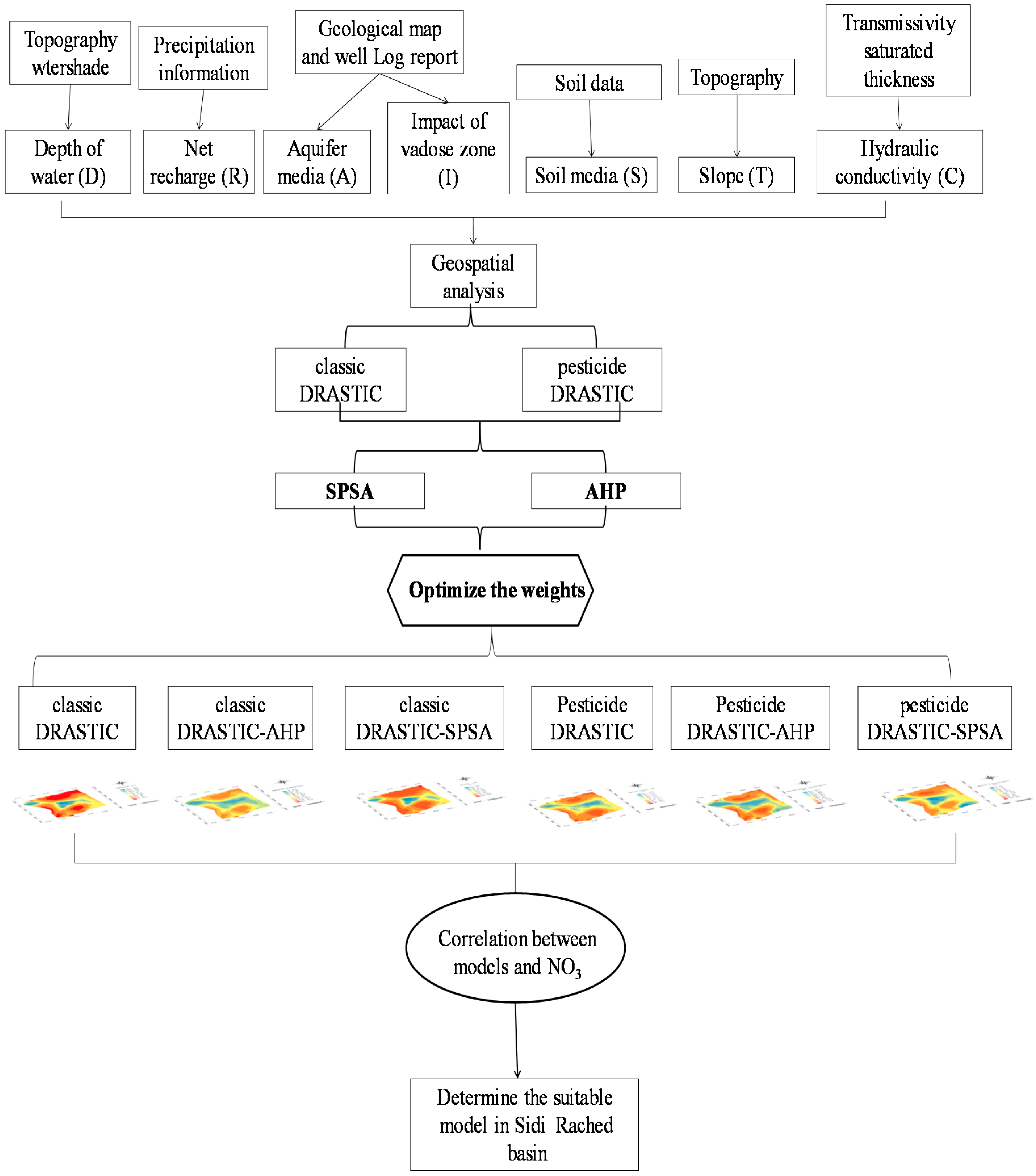
4.1. Preparation and Processing of Data

The DRASTIC model with its seven parameters was derived from several data sets, the sources of which are presented in Table 2.

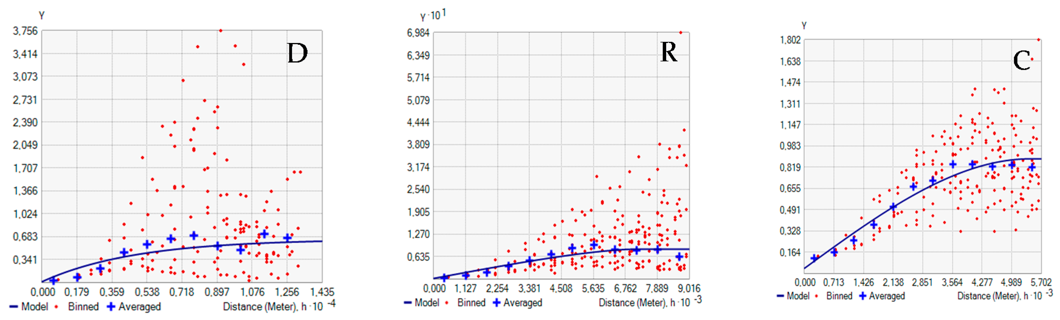
Depth to water: Water table depths were obtained from boreholes provided by National Agency of Hydraulic Resources (ANRH). Data was extrapolated to the whole study area by using the kriging ordinary technique from the geostatistical extension “spatial analyst” of ArcGIS 10. The choice of the best surface was made based on the comparison of the different interpolation methods by the application of the cross-validation technique. The evaluation criteria are based on Mean Error (ME ≅ 0) values and root-mean square standardized error (RMSE ≅ 1) values. The exponential semivariogram model was the best-fitting model (Figure 6 and

Table 5. Summary of the best-fit models for parameters Depth to water, net Recharge and hydraulic Conductivity.

Parameter	Model	Nugget Effect	Sill (C0 + C)	Mean	RMS	RMSS
D (m)	Exponential	0.012	0.519	0.0016	0.428	1.19
R (mm/year)	Circular	0.002	0.078	0.0011	0.073	0.67
C (m/s)	Spherical	0.039	0.842	0.0015	0.384	0.98

RMS: Root mean square, RMSS: Root mean square standardized.

). A raster with the depth to water of the study area was reclassified into vulnerability values according to each height. The values range between 0.7 and 74.6 m. The average depth to water of the study area is 27.89 m (a shallow groundwater system), with a standard deviation of 12.69 m (Table 4). Moreover, in Table 4, the skew value is equal to 0.316, indicating that the distribution is moderately skewed with an asymmetric tail extending toward positive values. The calculated kurtosis value (3.052) is approximately 3, indicating that the distribution is normal. The parameters used in the interpolation and the associated semivariogram are shown in Table 5 and Figure 6.

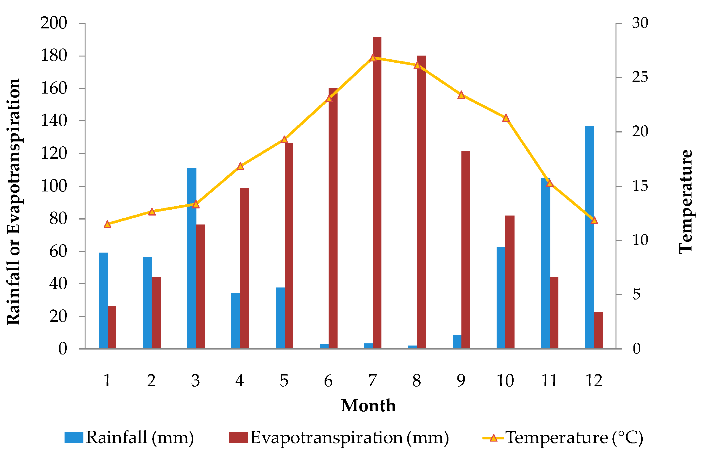
Net recharge: Net recharge (R) represents the amount of water per unit area of land which penetrates the ground surface and reaches the water table. This recharge water is thus available to transport a contaminant vertically to the water table and horizontally within the aquifer [24]. In addition, the quantity of water available for dispersion and dilution of the contaminant in the vadose zone and in the saturated zone is controlled by this parameter [9]. Net recharge values were estimated based on precipitations by applying the model established by Mac Donald (1992) as a result of the hydroagricultural study of Mitidja plain, as follows: R = (P − RT) × RP. This net recharge data was then extrapolated to the whole watershed area by using the kriging ordinary technique from Arcgis10. The best-fitting theoretical models and related semivariogram parameters were chosen to obtain the most accurate estimation, by evaluating eleven different models. The cross-validation was undertaken and estimated the net recharge values in the aquifer, and the circular semivariogram model was the best-fitting model (Figure 6 and Table 5). The cross-validation, which represents the accuracy of the predictions, shows that the mean error is close to 0 (0.0011) and that the standardized root mean square is close to one. The average annual net recharge values fluctuate considerably from one borehole to another, varying between an interval of 30 mm and 125 mm. The study area is characterized by an annual average rainfall ranging from 500 to 600 mm. More than 60% of the study area has low groundwater recharge rates (30–90 mm/year). The average annual net recharge of the study area is 78.88 mm with a coefficient of variation of 0.218 and a standard deviation of 17.19 mm (Table 4). A skewness and kurtosis test were applied to characterize the net recharge (R) frequency and its distribution shape; the skew value obtained is equal to 0.44, indicating that the distribution is moderately skewed with an asymmetric tail extending toward positive values. The calculated kurtosis value is 3.02, indicating that the distribution is normal. The parameters used in the interpolation and the associated semivariogram are shown in Table 5 and in Figure 6.

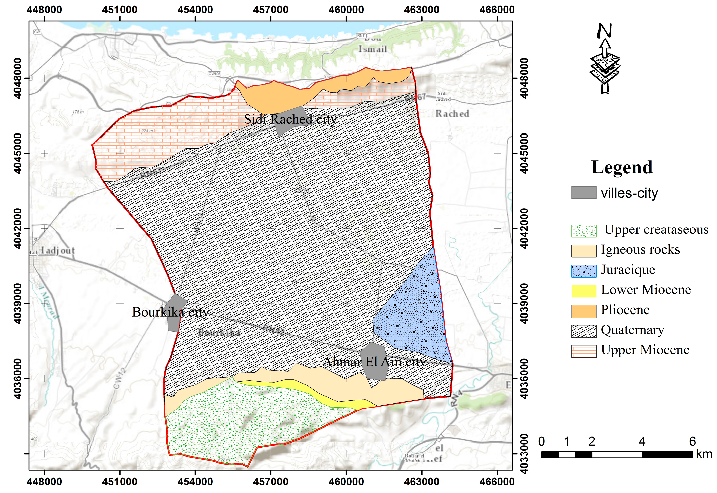
Aquifer Media: This parameter represents the geological formation of the aquifer in the upper layer; it is prepared from the hydrogeological map and profiles of the boreholes. It governs the time and path followed by the contaminant to reach the water table; various formations have different degrees of permeability of the aquifer. The aquifer of Sidi Rached consists mainly of gravel and clay, clay and gravel, alluvium (mixture of clay, sand and gravel) of sand and limestone–marl and marl and clay. Index values were determined according to the classes reported in Table 2.

Soil: The soil has a considerable impact on groundwater contamination by pollutants from the surface. It can reduce, delay or accelerate the spread of pollutants to the aquifer. The more soil is rich in clay, the more absorption of pollutants is important, and the more protection of groundwater is high. The information gathered from studies and soil maps has defined the nature of the soil. Index values were determined according to the classes reported in Table 2. The distribution of soil taxonomy was obtained from digitalized soil maps of the Sidi Rached basin. Moreover, each soil subgroup was related to its texture according to study carried out in the area. The texture of subgroups was translated to DRASTIC ratings using Table 2 [24].

Topography: Topography is represented in DRASTIC by the slope of the land surface. At steep slopes, contaminants tend to move with the runoff water and therefore there is less pollutant retention and in turn little infiltration of contaminants will take place. On the other hand, shallow slopes have more potential for pollutant retention and in turn infiltration of contaminants. Then, the slope index was reclassified and converted into grid coverage and multiplied by the topographic weight. A model of the digital elevation study area ASTER GDEM version 2 of 30 m resolution was used in this study to calculate the percent slope. The slope was then classified according to the ranges criteria in Table 2 via the ArcGIS 10. The topography map displayed a gentle slope (less than 6%) over most of the study area. The slope increases strongly in the south of the study area near the Blidean mounts.

Impact of the vadose zone: The vadose zone is defined as that above the water table which is unsaturated or discontinuously saturated. The nature of this area is an important parameter in the assessment of vulnerability, because it affects the speed of propagation of pollutants to the aquifer similar to the aquifer media (A). Its impact is determined from the lithology of land that constitutes it. The process of calculation and mapping theme “I” is the same as that of the saturated zone (A). It is obtained by the correlation of drill data and digitization of the geological map (scale 1/50,000). Different classes thus obtained are weighted from 1 to 9 by the DRASTIC model, with different degrees of vulnerability.

Hydraulic conductivity: The hydraulic conductivity values used to calculate the degree of vulnerability in our study area are obtained from pumping tests (are available as transmissivity). This net recharge data was then extrapolated to the whole watershed area by using the kriging ordinary technique from Arcgis10. The interpolation of the hydraulic conductivity calculated by Equation (3) allowed us to map the “C” parameter. The cross-validation was undertaken and the spherical semivariogram model was the best-fitting model (Figure 6 and

Table 6. Rating and weighting values used in the MDC, MDP, MDC–SPSA, MDP–SPSA, MDC–AHP and MDP–AHP models.

Parameters	Sub Parameters	r	MDC						MDP
			MDC		MDC-SPSA		MDC-AHP		MDP		MDP-SPSA		MDP-AHP
			w	Total	w	Total	w	Total	w	Total	w	Total	w	Total
Depth to water (m)	0–2	10		50		35		50		50		27		50
	2–6	9		45		31.5		45		45		24.3		45
	6–12	5	5	25	3.5	17.5	5	25	5	25	2.7	13.5	5	25
	12–18	3		15		10.5		15		15		8.1		15
	>18	1		5		3.5		5		5		2.7		5
Net Recharge (mm)	0–50	1		4		3.8		3		4		2.9		2.5
	50–100	3	4	12	3.8	11.4	3	9	4	12	2.9	8.7	2.5	7.5
	100–178	6		24		22.8		18		24		17.4		15
Aquifer Media	Alternating of gravel and clay	7		21		32.9		12.6		21		23.8		9.8
	Alluvium (mixture of clay, sand and gravel)	6	3	18	4.7	28.2	1.8	10.8	3	18	3.4	20.4	1.4	8.4
	Limestone clay and sand	4		12		18.8		7.2		12		13.6		5.6
	Clay and gravel	3		9		14.1		5.4		9		10.2		4.2
	Marl and clay	2		6		9.4		3.6		6		6.8		2.8
Soil Media	Non clay	1		2		2.2		1.2		5		3.7		5
	Clay-loam	3		6		6.6		3.6		15		11.1		15
	Clay-silty limestone	5	2	10	2.2	11	1.2	6	5	25	3.7	18.5	5	25
	Silt-clay limestone	6		12		13.2		7.2		30		22.2		30
	Alluvial calcareous and stones	7		14		15.4		74		35		25.9		35
Topography (%)	0–2	10		10		25		10		30		50		14
	2–6	9		9		22.5		9		27		45		12.6
	6–8	8		8		20		8		24		40		11.2
	8–10	7	1	7	2.5	17.5	1	7	3	21	5	35	1.4	9.8
	10–12	5		5		12.5		5		15		25		7
	12–18	3		3		7.5		3		9		15		4.2
	>18	1		1		2.5		1		3		5		1.4
Impact of vadose zone	Clay and little sandstone	1		5		5		5		4		3		2.5
	Clay at low percentage of gravel	2	5	10	5	10	5	10	4	8	3	6	2.5	5
	Clay and gravel	4		20		20		20		16		12		10
	Sandstone and clay	6		30		30		30		24		18		15
Hydraulic Conductivity (m/s)	0.047 × 10−5–4.7 × 10−5	1		3		1		1.8		2		1		1
	4.7 × 10−5–14.7 × 10−5	2	3	6	1	2	1.8	3.6	2	4	1	2	1	2
	14.7 × 10−5–32.9 × 10−5	4		12		4		7.2		8		4		4

). The cross-validation, which represents the accuracy of the predictions, shows that the mean error of hydraulic conductivity is close to 0 (0.0015) and that the standardized root mean square is close to one (0.98). Three classes of hydraulic conductivity were distinguished and indexed according to the DRASTIC model. A class of low values (0.36 × 10⁻⁵ to 4.71 × 10⁻⁵ m/s) is located to the north-east of the basin and represents only 2.24% of the total area; another class of mean values (4.7 × 10⁻⁵ and 14.7 × 10⁻⁵ m/s). Furthermore, a last class of high values is located north-west and south-west of the study area. The average hydraulic conductivity of the study area is 3.43 × 10⁻⁵ m/s with a coefficient of variation of 0.933 and a standard deviation of 3.197 × 10⁻⁵ m/s (Table 4).

4.2. Classic DRASTIC and Pesticide DRASTIC Models

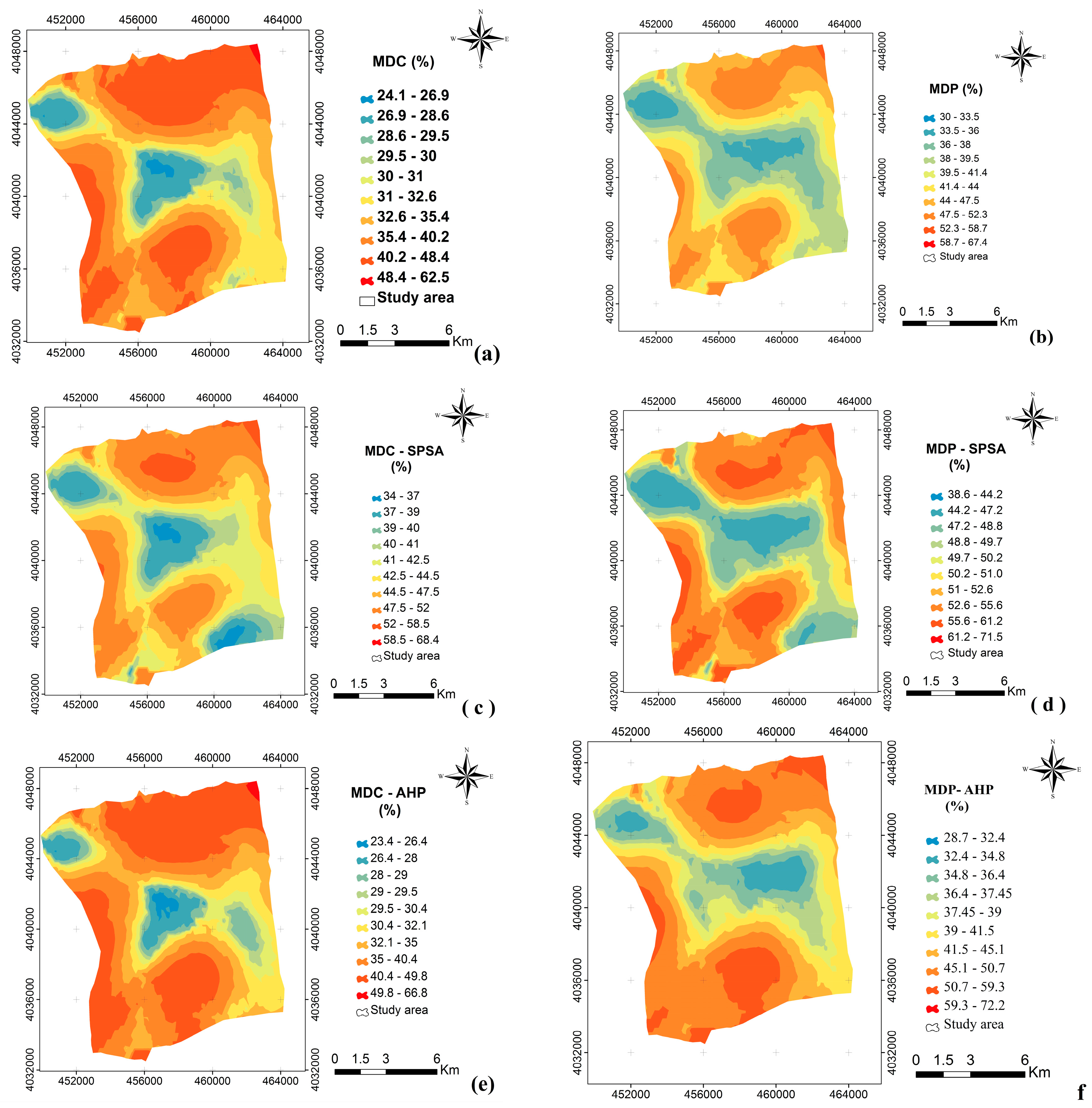
The ratings were attributed to the parameters taking into account their information and data which are presented in Table 2 and are depicted in Table 6. The vulnerability index of classic DRASTIC obtained was between 72 and 150; the spatial distribution is illustrated in Figure 7a. Three (03) classes of vulnerability were identified: (i) a class of low vulnerability occupying 65.4% of the total area of basin, located in the centre of the basin, northwest of the Sidi Rached city and southeast of the study area. That may be explained by the low permeability (0.4–2 × 10⁻⁵ m/s) and low recharge (50–80 mm/year) in the centre and by the soil type (clay–loam–calcareous) and impact of the vadose zone (clay and sandstone) in the extremities of the basin area (northwest and southeast); (ii) a second class of medium vulnerability to pollution, occupying 32.1% of the study area; (iii) and a third class of high vulnerability, located near the city of Sidi Rached, Bourkika and Ahmar El Ain, representing 2.5% of the study area. The high vulnerability may be explained by the low depth to water (0.6–4 m) at the nearest city of Sidi Rached, by the high recharge (90–125 mm/year) and by the fact that agriculture is familiar, extensively using nitrogen fertilization.

The pesticide DRASTIC model uses the same thematic maps and the same grading as MDC but the weights of assigned parameters correspond to the MDP model [24] (Table 2). The vulnerability indexes of the pesticide DRASTIC model thus obtained were between 95 and 181 (Figure 7b). This later allowed the definition of (03) three vulnerability classes: (i) a class of low vulnerability occupying 50% of the basin and located in its central part, northwest of the Sidi Rached city and at the southeast of the study area; (ii) a medium class occupying 38% of the study zone; and (iii) a high vulnerability class, occupying 12% of the global surface of the basin. It can be seen that the results are similar for both models except that values of the medium and high classes yielded by the pesticide DRASTIC model were superior to those of the classic DRASTIC model. This indicates the good capacity of the MDP model for diagnosing vulnerable areas and confirms the existence of a rural population in this part of the basin.

4.3. Optimized DRASTIC Models

In order to put forward a more realistic method to classify the groundwater vulnerability, the weights of the parameters of the classic DRASTIC and pesticide DRASTIC models were modified using two techniques: single parameter sensitivity analysis (SPSA) and Analytic hierarchic process (AHP). The weights of the parameters, thus obtained (

Table 7. The weights of the parameters obtained by SPSA and AHP. SPSA: Single-Parameter Sensitivity Analysis, AHP: Analytic Hierarchy Process.

Weights of the Parameters	D	R	A	S	T	I	C
MDC–SPSA	0.15	0.17	0.21	0.10	0.11	0.22	0.04
MDP–SPSA	0.12	0.13	0.16	0.18	0.25	0.14	0.02
MDC–AHP	0.31	0.16	0.08	0.04	0.02	0.31	0.08
MDP–AHP	0.30	0.13	0.06	0.30	0.06	0.13	0.03

), were introduced into Equation (3) to calculate the vulnerability index (MDC–SPSA, MDC–AHP, MDP–SPSA and MDP–AHP).

According to these results, the impact of the vadose zone and the topography are the most important factors of vulnerability obtained by the application of the SPSA technique for the MDC and MDP respectively, while the hydraulic conductivity is the least important for both models (see Figure 7c,d). According to the results of the AHP adjustment, the depth of the aquifer and the impact of the vadose zone are the parameters which have the highest weight for the MDC, whereas for the MDP, it is the impact of the vadose zone, type of soil (S) and the depth of the water which have the highest weights. On the other hand, the lowest parameters are the type of soil and the hydraulic conductivity for the MDC and MDP respectively (see Figure 7e,f). The weight of the hydraulic conductivity factor (MDC–SPSA, MDP–SPSA and MDP–AHP) and type of soil (MDC–AHP) are rather small so the impact of this parameter in the related vulnerability index is residual. According to some authors [19,29], the redundant parameters must be eliminated from the vulnerability equations because it simplifies vulnerability assessments. However, this reasoning was not followed because we seek a comparison of the parameters’ weights resulted from the two adjustment techniques. The coefficients of Table 7 are harmonized in a range of 1 to 5 (

Table 8. Models and harmonized weights.

Factors and Index	Model and Harmonized Weights
	Classic DRASTIC (MDC)			Pesticide DRASTIC (MDP)
	MDC	MDC–SPSA	MDC–AHP	MDP	MDP–SPSA	MDP–AHP
D	5	3.5	5.0	5	2.7	5.0
R	4	3.8	3	4	2.9	2.5
A	3	4.7	1.8	3	3.4	1.4
S	2	2.2	1.2	5	3.7	5
T	1	2.5	1	3	5.0	1.4
I	5	5.0	5.0	4	3	2.5
C	3	1	1.8	2	1	1
Minimal index	72	91	58	95	96	61
Maximal index	150	159.3	129.5	181	159	136

).

The vulnerability index derived from the adjustment of the MDC and MDP parameters are listed in Table 5 and comply with the following intervals: 72 ≤ MDC ≤ 150; 91 ≤ MDC–SPSA ≤ 159.3; 58 ≤ MDC–AHP ≤ 129.96; 95 ≤ MDP ≤ 181; 96≤ MDP–SPSA ≤ 159 and 61 ≤ MDP–AHP ≤ 136. In both cases, SPSA predicts the highest vulnerabilities and AHP the lowest. The corresponding vulnerability maps are illustrated in Figure 7c–f.

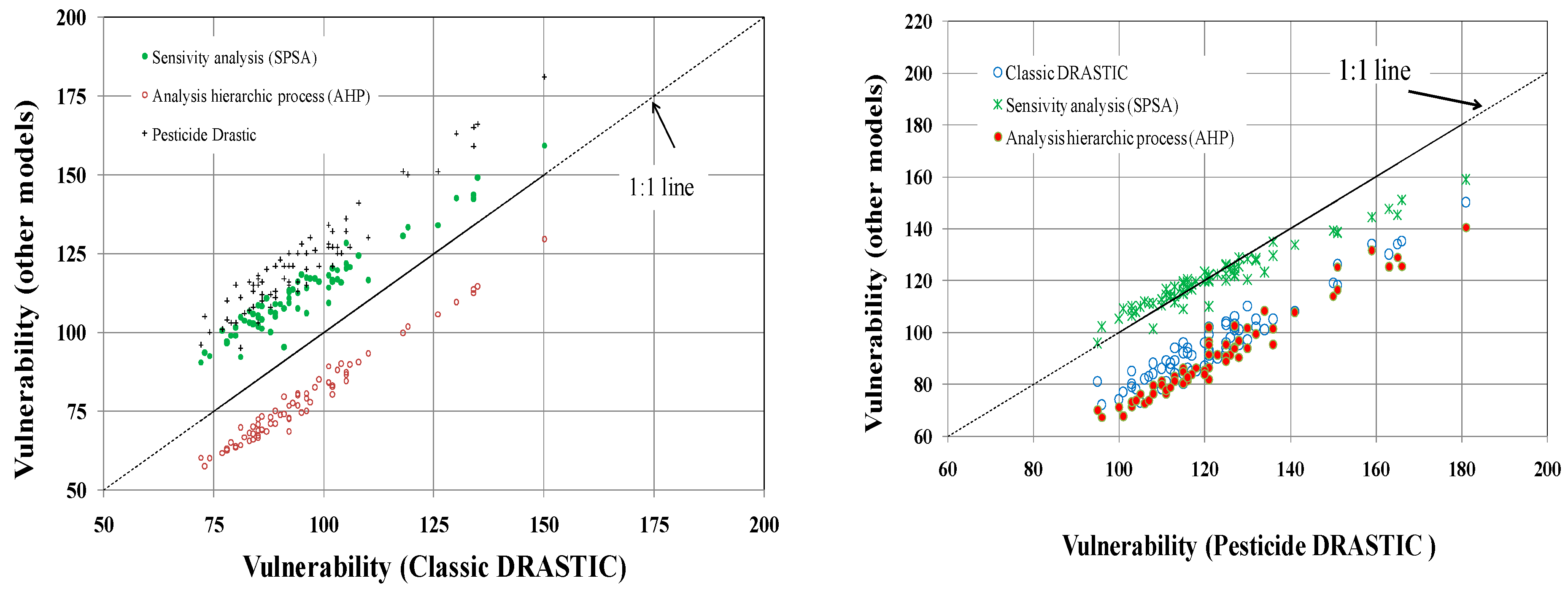
4.4. Comparison between Vulnerability Indexes

Comparisons of the indexes arising from the adjustments applied to the parameters of MDC and MDP, with regard to the original (MDC and MDP), were performed (Figure 8). The results show that the new MDC indexes estimated by the hierarchical analysis (AHP) deviate from the 1:1 line towards lower values with a rate that varies from 6% to 11%, and the indexes estimated by the single-parameter sensitivity analysis (SPSA) deviate towards higher values with a rate ranging from 3% to 13%. These adjustments are not constant but depend linearly on the MDC (Figure 8).

MDC (SPSA) = 0.8 MDC + 35 (R = 0.93) and MDC (AHP) = 0.9 MDC − 8.8 (R = 0.97). However, the MDP index moves from the line 1:1 with a constant average margin of 25 points, because the confidence line adjusted to the dispersion points is parallel to the line 1:1, where the relationship between MDC and MDP is as follows: MDP = MDC + 25 (R = 0.92).

The MDP–AHP indexes deviate from the line 1:1 to lower values with a rate that varies from 15 to 33% (Figure 7). However, the MDP–SPSA indexes deviate slightly from the line 1:1 (+ 8% to −12%). These adjustments depend linearly on the MDP (pesticide DRASTIC model): MDP (SPSA) = 0.66 MDP + 41 (R = 0.94), MDP (AHP) = 0.9 MDP − 21 (R= 0.95) and MDC = MDP − 25 (R = 0.92). Globally, the vulnerability indexes estimated by the models arising from weighting adjustments in the study zone deviate from the line 1:1 (MDC or MDP) with an average value of 20 points for a maximum value of 41 points. These differences represent an uncertainty of one to two classes of vulnerability, which are 20 points wide (Figure 8). They can be explained by the difference of a model compared to the original models (MDC and MDP), and they pose the problem of consistency between the different techniques.

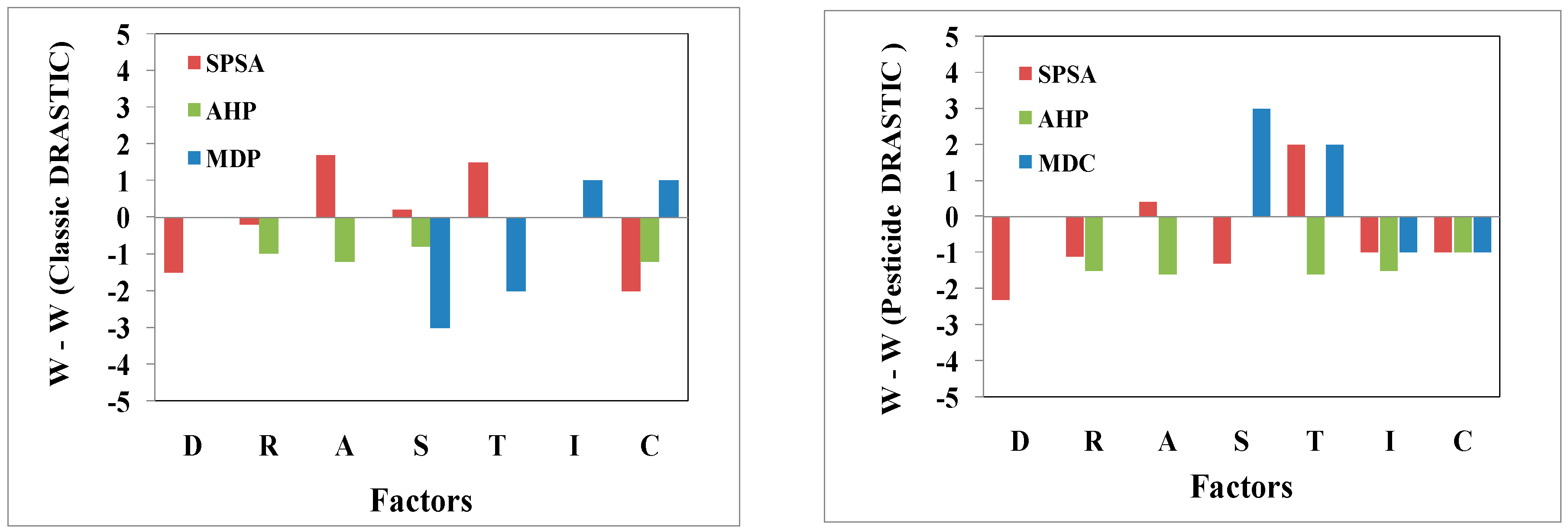
4.5. Comparisons among Weights

The variations in the weights estimated by Sensitivity Analysis and AHP, relative to the original DRASTIC values, were deduced from the data in Table 6 and summarized in Figure 9a,b. The largest difference in weight was observed between the MDC and MDP at the level of WS (around 3). The results obtained by the AHP process are either equal (WD, T and WI) or much lower than those obtained with the classic DRASTIC model (varies between −1.2 and −0.8); the underestimated parameter weights are WR, WA, WS and WC. Furthermore, the parameters that have the highest weights (=5) were not modified, namely D and I. The AHP technique retains the major importance of WD, WI and WT with slight reductions of other factors. Similar results were obtained by other authors [13,30,31]. However, the weights resulting from the sensitivity analysis are different from the DRASTIC weights (MDC) except for WI (=5). Several studies have led to the same conclusions [10,14,32].

A comparison of the parameters’ weights of classic DRASTIC with the harmonized weights resulting from the application of the adjustment techniques AHP and the sensitivity analysis was performed (Figure 9). The results show that the WD, WI, and the WD, WT are almost unchanged, contrary to the residual variations in the other parameters (

Table 9. Correlation coefficients between the various indexes of vulnerabilities and the nitrates (Boldface coefficients are significant for p < 0.05).

	NO3−	MDC	MDC–SPSA	MDC–AHP	MDP	MDP–SPSA	MDP–AHP
NO3−	1.00
MDC	0.60	1.00
MDC–SPSA	0.65	0.96	1.00
MDC–AHP	0.67	0.97	0.92	1.00
MDP	0.64	0.96	0.95	0.92	1.00
MDP–SPSA	0.68	0.89	0.95	0.83	0.97	1.00
MDP–AHP	0.72	0.94	0.89	0.90	0.97	0.91	1.00

). WI and the WD, WT have practically not changed; on the other hand, the weights of the other parameters have undergone changes of 0.2 to 2. The indexes calculated by AHP are highly correlated (R = 0.98 and 0.97 respectively for the MDC and MDP) compared with those calculated by the sensitivity analysis (R = 96 and R = 97 respectively for the MDC and MDP). The results obtained with the AHP technique on classic DRASTIC are significantly lower than those obtained by the pesticide DRASTIC model, except for WD and WS, or their initial weights were kept. The AHP technique maintains the importance of the highest parameters of both cases MDC (D and I) and MDP (D and S). Slight decreases were observed in the other parameters. The weights obtained by the sensitivity analysis technique were significantly lower than those of MDP except for WA and WT weights where we note an increase of 1.7 and 1.5 respectively. A final comparison between the original models (MDC and MDP) and the models resulting from weightings adjustment was carried out by calculating the correlation coefficients between the vulnerability indexes (Table 9) where a good correlation between the different indexes of vulnerability was found (0.89 ˂ r ˂ 0.98).

4.6. Validation of the Vulnerability Index

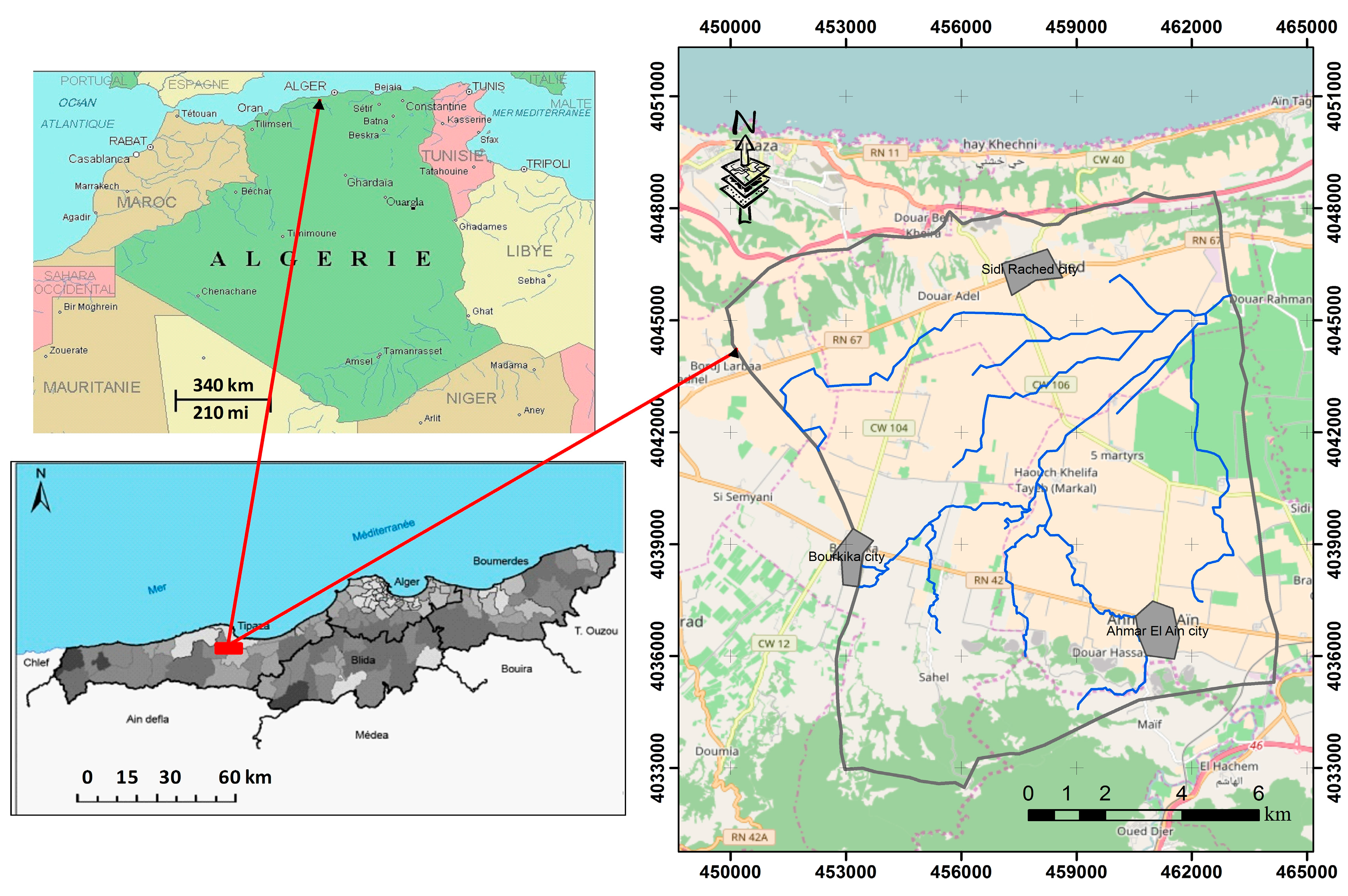
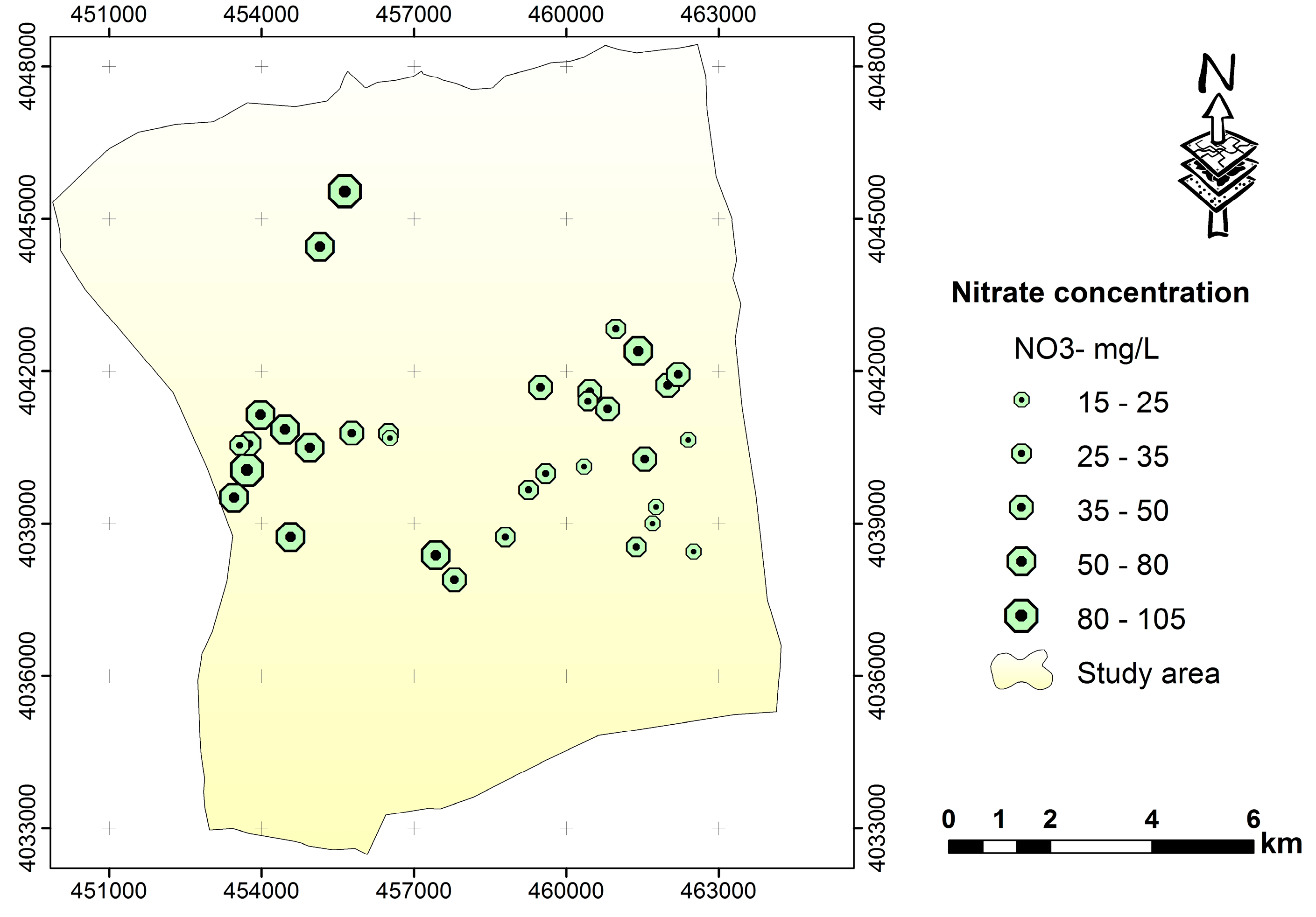
The nitrate concentration was selected as the main parameter of the initial contamination to validate the original DRASTIC (MDC and MDP) models and the models resulting from the adjustment (SPSA–MDC, MDC–AHP, SPSA–MDP and MDP–AHP). Nitrate has been chosen because the study area is characterized by active agriculture, it is a good indicator for groundwater quality and its data is available. Data on the nitrate concentration refers to three measuring years: 2007, 2008 and 2009. 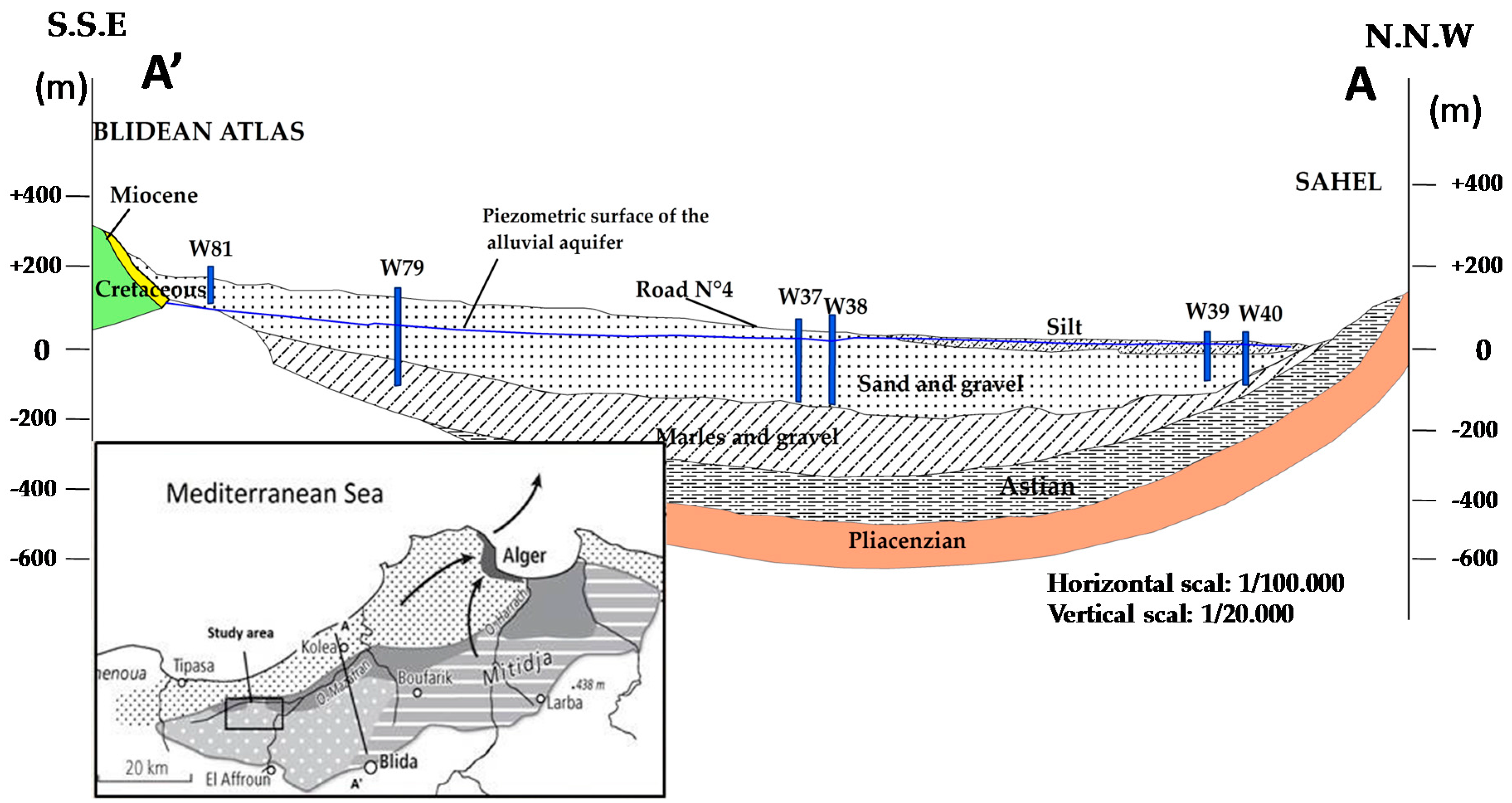A total of 34 boreholes that existed in the study area (Sidi Rached plain) are selected as sampling locations for the Nitrates analysis (Figure 10). They are located in the aquifer alluvial quaternary (unconfined aquifer) with variable depths ranging from 50 to 100 m; this is in order to avoid intra-borehole artificial mixing which can often occur in wells, masking the real geochemistry of the aquifer. This phenomenon especially increases in the presence of old groundwater residing below younger groundwater in thick aquifers or oxidoreducing environments. The samples were collected with great care during low-flow pumping, in order to obtain samples with minimum disturbance from the in situ geochemical and hydrogeological conditions. In the case of the Sidi Rached plain where the study area is located, the wells are usually shallow so the assumption of homogeneity within the screen can be considered acceptable for a large-scale study. In addition, these boreholes have between two to five screens located at different levels depending on the constituents of the aquifer, the length of which varies from 6 to 20 m. Consequently, a uniform stratigraphic exists across these screened intervals. The samples collected were preserved in polyethylene bottles at low temperature and transferred to the laboratory ANRH (National Agency for Water resources) for the analysis.

Fundamental Statistics tests for nitrate concentrations were applied to characterize the location and variability of a data set (

Table 10. Summary statistics of nitrate data.

Parameters	NO3− (mg/L)
Minimum	15.1
Maximum	104.6
Mean	44.4
First quartile	28.6
Third quartile	59.2
Standard error	3.7
Variance	448.7
Average deviation	17.0
Standard deviation	21.2
Coefficient of variation	0.5
Skew	1.0
Kurtosis	0.6
Kolmogorov–Smirnov (K–S) stat	0.2
Critical K–S stat, alpha = 0.5	0.2

); as can be seen, the nitrate concentration values fluctuate from one borehole to another varying between intervals of 15 and 104.6 mg/L. The average nitrate concentration in the study area is 44.4 mg/L, with a coefficient of variation of 0.5 and a standard deviation of 21.2 mg/L at the confidence interval of 0.95. The computed Kolmogorov–Smirnov test value (K–S = 0.2) at null hypothesis was less than the corresponding critical value of significance (p = 0.654). Thus, the hypothesis regarding the distributional shape is not rejected, as the K–S value is smaller than the critical value of significance. In addition, as can be seen in Table 10, the skew value is equal to 1.0, indicating that the distribution is moderately skewed with an asymmetric tail extending toward positive.

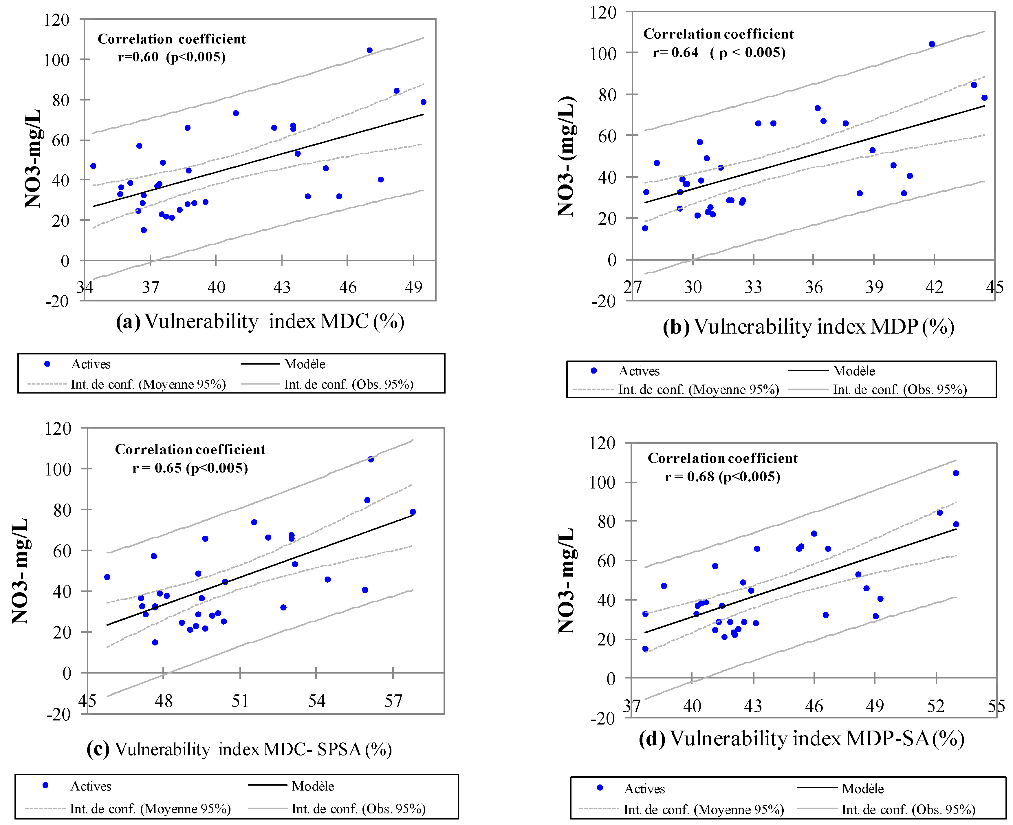
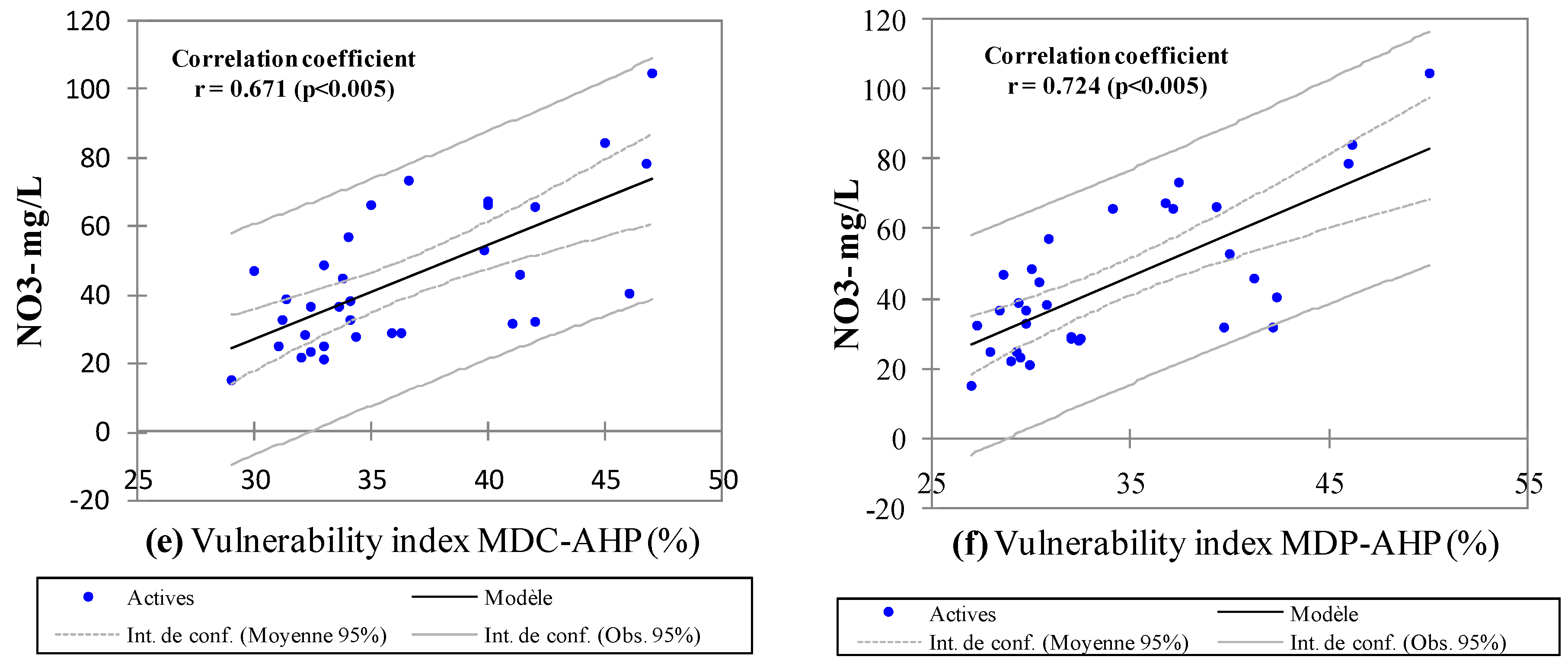
The correlations between the parameters are developed based on Pearson’s correlation method. The vulnerability indexes MDC–SPSA, MDP–SPSA, MDC–AHP and MDP–AHP are correlated with the nitrate concentrations of ground waters; we obtained 0.65, 0.68, 0.67 and 0.724 respectively. A significant improvement in the values of the correlation coefficient (R) was detected (Figure 11), with regard to the original DRASTIC models MDC and MDP, which were of 0.60 and 0.64 respectively.

The best correlation is that of MDP–AHP (R = 0.724) followed by MDP–SPSA (R = 0.68). This shows that the MDP model best explains the vulnerability index which coincides with other studies. Nitrate concentrations were found to be in the range of 15–104.6 mg/L and the average is close to the allowed limit (44.4 mg/L). The vulnerability index values of the corresponding points were determined from vulnerability index maps (Figure 7a–f). Calculated coefficient values are always much greater than Pearson’s critical value. Therefore, correlations are highly significant at the 1% probability level. The selection of a model to quantify the vulnerability in a region is not a straightforward task, requiring expertise and additional information to be set satisfactorily because one bad choice may lead to excessive constraints in regions forecasted as highly vulnerable.

Our choice was made according to two criteria: (i) have a better correlation between the vulnerability index and nitrate concentrations; (ii) weights must be proportional to the range of the ratings [33]. In this case, the recommended model to quantify the vulnerability in the study area (Sidi Rached) would be MDP–AHP.

5. Conclusions

Although there are several different models to assess groundwater vulnerability, there is no universal model for groundwater vulnerability assessment. The selection of models with which the groundwater vulnerability is going to be assessed depends mainly on the hydrogeological settings of the natural system and on data availability. The DRASTIC index is the most popular index method used to assess groundwater vulnerability to pollutions. However, it is also the method which is subjected to different forms of adjustment, and therefore constitutes a target for the strongest criticism among hydrogeologists. The Classic DRASTIC model has no ability to assess groundwater vulnerability for a specific pollutant or a particular hydrogeological feature; that is why an assessment of the vulnerability to nitrate of the Mitidja aquifer was conducted by applying two models: classic DRASTIC (MDC) and pesticide DRASTIC (MDP). Moreover, a modification of the original MDC and MDP algorithms was introduced. Thus, the new values of the weights of seven parameters forming the MDC and MDP were calculated using two weighting techniques, namely: Analysis Hierarchic Process (AHP) and Sensitivity Analysis (SPSA). The resulting models were MDC–SPSA, MDP–SPSA, MDC–AHP and MDP–AHP. Classic DRASTIC vulnerabilities ranged from 72 (low) to 150 (high), whereas the pesticide DRASTIC vulnerability ranged from 95 (low) to 181 (high).

The adjustment of the weights of the classic DRASTIC and pesticide DRASTIC models by Sensitivity Analysis (SPSA) resulted in vulnerability indexes that were on average 12.7% higher than the original DRASTIC values, and a reduction of 7% for the pesticide DRASTIC model. However, the adjustment of the weights by AHP resulted in vulnerability indexes that were on average 12.7% and 25% lower than the original DRASTIC values for MDC and MDP respectively. This reduction can be explained by the modifications made in the weighting factors (w). Parameters’ weights adjustment by the AHP technique, in the case of pesticide DRASTIC, produced highly correlated results (%) better than classic DRASTIC. AHP retains the highest weight of/for (D) and (I) factors and the lowest weights for the remaining factors. The sensitivity analysis reduced the importance of the weight factors of D (1.5) and C (2), and increased the importance of the weight factors of A (1.7) and T (1.5) qualified by the classic DRASTIC model, while other weights (R, S and I) remained almost unchanged. Similar results have been previously reported in other regions. The correlation coefficients between the original vulnerability index and nitrate concentrations were 0.60 and 0.64 for MDC and MDP respectively, while the correlations resulting from the four adjustment models ranged between 0.65 and 0.72 (Table 9). The calculations showed that the best model resulted from the MDP–AHP combination followed by MDC–AHP, MDP–SPSA, MDC–SPSA, MDP and finally MDC. In conclusion, this work demonstrated that the MDP–AHP vulnerability map constitutes an excellent decision-making and space analysis help tool for feasibility study projects and the development of agricultural and environmental activities in the study area (Sidi Rached basin). Also, these results can be exploited in similar areas such as some parts of the Middle East and North Africa “MENA”.

References

1. Boudjellal, A.A.; Bekkar, Y.; Kuper, M.; Errahj, M.; Hammani, A.; Hartani, T. Analyse des arrangements informels pour l’accès à l’eau souterraine sur les périmètres irrigués de la Mitidja (Algérie) et du Tadla (Maroc). Cah. Agric. 2011, 20, 85–91. (In French) [Google Scholar]
2. Rached, S. Hydrologie de la Nappe de la Mitidja (Algérie): Etude Hydrodynamique des Champs Captants de la Ville d’Alger. Ph.D. Thesis, Géologie Appliquée, Université Scientifique et Médicale de Grenoble Français, Grenoble, France, 1986. [Google Scholar]
3. Imerzoukene, S. Hydrogeochemie et Simulation de l’Ecoulement des eaux Souterraines et de la Position de l’Interface eau Douce-Eau Salée dans la Partie Est de la Plaine de la Mitidja (Algérie). Ph.D. Thesis, Katholieke Universiteit Leuven, Leuven, Belgium, 1995; p. 273. [Google Scholar]
4. Cavero, J.; Barros, R.; Sellam, F.; Topcu, S.; Isidoro, D.; Hartani, T.; Lounis, A.; Ibrikci, H.; Cetin, M.; Williams, J.-R.; et al. APEX simulation of best irrigation and N management strategies for off-site N pollution control in three Mediterranean irrigated watersheds. Agric. Water Manag. 2012, 103, 88–99. [Google Scholar] [CrossRef]
5. Frink, C.R. Estimating Nutrient Exports to Estuaries. J. Environ. Qual. 1991, 20, 717–724. [Google Scholar] [CrossRef]
6. Novotny, V. Diffuse pollution from agriculture in the world. In Proceedings of the International Workshop on Where do Fertilizers Go? Belgirate, Italy, 28–29 June 2005. [Google Scholar]
7. Focazio, M.J.; Reilly, T.E.; Rupert, M.G.; Helsel, D.R. Assessing Ground-Water Vulnerability to Contamination: Providing Scientifically Defensible Information for Decision Makers; U.S. Geological Survey Circular-1224; USGS: Reston, VA, USA, 2002; p. 33.
8. Sinan, M.; Razack, M. An extension to the DRASTIC model to assess groundwater vulnerability to pollution: Application to the Haouz aquifer of Marrakech (Morocco). Environ. Geol. 2009, 57, 349–363. [Google Scholar] [CrossRef]
9. Napolitano, P.; Fabbri, A.-G. Single parameter sensitivity analysis for aquifer vulnerability assessment using DRASTIC and SINTACS. In Proceedings of the Hydro GIS: Application of Geographical Information Systems in Hydrology and Water Resources Management, Vienna, Austria, 16–19 April 1996; Kovar, K., Nachtnebel, H.P., Eds.; IAHS Publication: Wallingford, UK, 1996; Volume 235, pp. 559–566. [Google Scholar]
10. Almasri, M.-N. Assessment of intrinsic vulnerability to contamination for Gaza coastal aquifer, Palestine. J. Environ. Manag. 2007, 88, 577–593. [Google Scholar] [CrossRef] [PubMed]
11. Neshat, A.; Pradhan, B.; Dadras, M. Groundwater vulnerability assessment using an improved DRASTIC method in GIS. Resour. Conserv. Recycl. 2014, 86, 74–86. [Google Scholar] [CrossRef]
12. Saaty, T.-L. The Analytic Hierarchy Process; McGraw-Hill: New York, NY, USA, 1980. [Google Scholar]
13. Sener, E.; Davraz, A. Assessment of groundwater vulnerability based on a modified DRASTIC model, GIS and an analytic hierarchy process (AHP) method: The case of Egirdir Lake basin (Isparta, Turkey). Hydrogeol. J. 2013, 21, 701–714. [Google Scholar] [CrossRef]
14. Neshat, A.; Pradhan, B.; Piraste, S.; Shafri, H.-Z.-M. Estimating groundwater vulnerability to pollution using a modified DRASTIC model in the Kerman agricultural area, Iran. Environ. Earth Sci. 2014, 71, 19–31. [Google Scholar] [CrossRef]
15. Neshat, A.; Pradhan, B.; Shafri, H.-Z.-M. An integrated GIS based statistical model to compute groundwater vulnerability index for decision maker in agricultural area. J. Indian Soc. Remote Sens. 2014, 76, 543–563. [Google Scholar] [CrossRef]
16. Pacheco, F.; Pires, L.-M.-G.-R.; Bessa Santos, R.; Sanches Fernandes, L.-F. Factor weighting in DRASTIC modeling. Sci. Total Environ. 2014, 505, 474–486. [Google Scholar] [CrossRef] [PubMed]
17. Afshar, A.; Marino, M.; Ebtehaj, M.; Moosavi, J. Rule based fuzzy system for assessing ground-water vulnerability. J. Environ. Eng. 2007, 133, 532–540. [Google Scholar] [CrossRef]
18. Bojórquez-Tapia, L.-A.; Cruz-Bello, G.-M.; Luna-González, L.; Juáre, L.; Ortiz-Pérez, M.-A. V-DRASTIC: Using visualization to engage policymakers in groundwater vulnerability assessment. J. Hydrol. 2009, 373, 242–255. [Google Scholar] [CrossRef]
19. Pacheco, F.-A.-L.; Sanches Fernandes, L.-F. The multivariate statistical structure of DRASTIC model. J. Hydrol. 2013, 476, 442–459. [Google Scholar] [CrossRef]
20. Achi, K.; Salem, A.; Combes, P.; Couchot, A.; Grenet, B.; Pradines, D. Carte hydrogéologique d’Algérie 1/200.000; ANRH (Agence Nationale des Ressources Hydrauliques): Alger, Algeria, 1973. (In French) [Google Scholar]
21. Mac Donald, M. et Partners Limited. Etude de l’aménagement hydro-agricole de la plaine de Mitidja. Analyse des ressources en sol/ AGID; Alger. 1991-92-93.-4B.A, ill; 30cm. Available online: http://mree.gov.dz/wp-content/uploads/2016/10/CATALOGUE-ETUDES-1.pdf (accessed on 30 March 2017).
22. Ecrement, Y.; Seghir, B. Etude agro pédologique de la Mitidja; ANRH (Agence Nationale des Ressources Hydrauliques): Alger, Algeria, 1971. (In French) [Google Scholar]
23. Compagnie Générale de Géophysique (CGG). Etude géophysique par prospection électrique dans la plaine de Nador, Tipaza; General Company of Geophysics, DMRH (Direction des études de milieu et de la recherche Hydraulique): Alger, Algeria, 1967. (In French) [Google Scholar]
24. Aller, L.; Lehr, J.-H.; Petty, R.-J.; Hackett, G. Drastic: A Standardized System for Evaluating Ground Water Pollution Potential Using Hydrogeologic Settings. Available online: http://rdn.bc.ca/cms/wpattachments/wpID3175atID5999.pdf (accessed on 24 March 2017).
25. Yin, J.-Y.; Long, X.-P.; Yuan, C.; Sun, M.; Zhao, G.-C.; Geng, H.-Y. A Late Carboniferous–Early Permian slab window in the West Junggar of NW China: Geochronological and geochemical evidence from mafic to intermediate dikes. Lithos 2013, 175, 146–162. [Google Scholar] [CrossRef]
26. Gogu, R.-C.; Hallet, V.; Dassargues, A. Comparison of aquifer vulnerability assessment techniques. Application to the Ne’blon river basin (Belgium). Environ. Geol. 2003, 44, 881–892. [Google Scholar] [CrossRef]
27. Huan, H.; Wang, J.; Teng, Y. Assessment and validation of groundwater vulnerability to nitrate based on a modified DRASTIC model: A case study in JilinCity of northeast China. Sci. Total Environ. 2012, 440, 14–23. [Google Scholar] [CrossRef] [PubMed]
28. Bhushan, N.; Rai, K. Strategic decision making. In Applying the Analytic Hierarchy Process; Springer: New York, NY, USA, 2004. [Google Scholar]
29. Journel, A.J.; Huijbregts, C.J. Mining Geostatistics; Academic Press: New York, NY, USA, 1978. [Google Scholar]
30. Zhang, Q.; Yang, X.; Yan, Z.; Ming, Z. Risk Assessment of Groundwater Contamination: A Multilevel Fuzzy Comprehensive Evaluation Approach Based on DRASTIC Model. Sci. World J. 2013, 2013, 610390. [Google Scholar] [CrossRef] [PubMed]
31. Akbari, G.-H.; Rahimi-Shahrbabakia, M. Sensitivity analysis of water at higher risk subjected to soil contaminations. Comput. Methods Civ. Eng. 2011, 2, 83–94. [Google Scholar]
32. Tirkey, P.; Gorai, A.-K.; Iqbal, J. AHP-GIS Based DRASTIC Model For Groundwater Vulnerability To Pollution Assessment: A Case Study Of Hazaribag District, Jharkhand, India. Int. J. Environ. Prot. 2013, 2, 20–31. [Google Scholar]
33. Malczewski, J. GIS and multicriteria decision analysis. Int. J. Geogr. Inf. Sci. 1999, 20, 703–726. [Google Scholar] [CrossRef]
Figure 1. Location map of the Sidi Rached plain.
Geosciences 07 00020 g001
Figure 2. Figure 2. Monthly averages of precipitation, temperature and evapotranspiration.
Geosciences 07 00020 g002
Figure 3. The geological map of the study area.
Geosciences 07 00020 g003
Figure 4. Geological cross section of Sahel and the Blidean Atlas (AA’) [20].
Geosciences 07 00020 g004
Figure 5. The flowchart of the methodology. SPSA: Single-Parameter Sensitivity Analysis, AHP: Analytic Hierarchy Process.
Geosciences 07 00020 g005
Figure 6. Adjusted theoretical variogram analysis for the Depth to water (D), net Recharge (R) and hydraulic Conductivity (C).
Geosciences 07 00020 g006
Figure 7. Vulnerability maps (af) based on various weighting factor methods (MPC, MDP, MDC–SPSA, MDP–SPSA, MDC–AHP and MDP–AHP).
Geosciences 07 00020 g007
Figure 8. Comparison of vulnerability indexes (adjusted models versus the MDC and MDP models).
Geosciences 07 00020 g008
Figure 9. Plot of the difference between classic DRASTIC and pesticide DRASTIC weights and homologous values estimated by the different adjustment techniques (SPSA and AHP).
Geosciences 07 00020 g009
Figure 10. The spatial distribution of the boreholes and their nitrate concentration.
Geosciences 07 00020 g010
Figure 11. Correlation between vulnerability indexes and nitrate concentration; (a) MDC–NO3; (b) MDP–NO3; (c) MDC–SPSA–NO3; (d) MDP–SPSA–NO3; (e) MDC–AHP–NO3 and (f) MDP–AHP–NO3.
Geosciences 07 00020 g011aGeosciences 07 00020 g011b