
Evaluation of Near-Surface Gases in Marine Sediments to Assess Subsurface Petroleum Gas Generation and Entrapment

Energy Futures Lab, Imperial College London, London SW7 2AZ, UK
Geosciences 2017, 7(2), 35; https://doi.org/10.3390/geosciences7020035
Submission received: 30 December 2016
/
Revised: 27 March 2017
/
Accepted: 10 April 2017
/
Published: 4 May 2017
(This article belongs to the Special Issue Natural Gas Origin, Migration, Alteration and Seepage)
Abstract
:Gases contained within near-surface marine sediments can be derived from multiple sources: shallow microbial activity, thermal cracking of organic matter and inorganic materials, or magmatic-mantle degassing. Each origin will display a distinctive hydrocarbon and non-hydrocarbon composition as well as compound-specific isotope signature and thus the interpretation of origin should be relatively straightforward. Unfortunately, this is not always the case due to in situ microbial alteration, non-equilibrium phase partitioning, mixing, and fractionation related to the gas extraction method. Sediment gases can reside in the interstitial spaces, bound to mineral or organic surfaces and/or entrapped in carbonate inclusions. The interstitial sediment gases are contained within the sediment pore space, either dissolved in the pore waters (solute) or as free (vapour) gas. The bound gases are believed to be attached to organic and/or mineral surfaces, entrapped in structured water or entrapped in authigenic carbonate inclusions. The purpose of this paper is to provide a review of the gas types found within shallow marine sediments and examine issues related to gas sampling and extraction. In addition, the paper will discuss how to recognise mixing, alteration and fractionation issues to best interpret the seabed geochemical results and determine gas origin to assess subsurface petroleum gas generation and entrapment.
1. Introduction
Seabed surface geochemical surveys are undertaken to investigate evidence of subsurface petroleum generation and entrapment [1,2]. The near-surface sediment gases can be derived from multiple sources including shallow microbial activity, thermal cracking of organic matter and inorganic materials or magmatic-mantle degassing. Gases derived from these different processes will display a distinctive hydrocarbon and non-hydrocarbon composition and compound-specific isotopic signature. Examination of seabed geochemical signatures from worldwide surveys suggest the near-surface sediment gas and isotopic signatures are different than expected due to in situ microbial alteration, partitioning between vapour, solute, and sorbed phases, mixing with gases from multiple origins, degassing fractionation from sample collection and fractionation related to the gas extraction method [2,3].
Sediment gases can reside in the interstitial spaces, bound to mineral or organic surfaces, and/or entrapped in carbonate inclusions [2,3]. The interstitial sediment gases are those gases contained within the sediment pore space, either dissolved in the pore waters (solute) or as free gas (vapour) [4]. The amount of gas dissolved in the pore waters or as a free phase vapour depends on pore water salinity, in situ temperature and pressure conditions and gas type (relative amount of non-hydrocarbon component and methane to ethane, propane, butane and pentane). The volume of gas dissolved in the pore waters or free as a vapour phase can be calculated using Henry’s law constant and an equation of state [4].
The bound gases are believed to be attached to organic and/or mineral surfaces, entrapped in structured water or entrapped in authigenic carbonate inclusions [3,5,6,7]. Horvitz [6,8] pioneered the concept of bound sediment gas analysis with his acid extraction adsorbed gas analysis. It was Horvitz’s belief that migrated thermogenic hydrocarbon gases readily bind to near-surface fine grained sediments (clays) due to the highly adsorptive nature of the clays towards hydrocarbons [6,8]. He also believed there was a preferential adsorption of the migrating thermogenic hydrocarbons relative to the in situ derived microbial gases [8,9]. Others have suggested that the binding process is related to structured water [7]. Whiticar [7] describes how structured water creates a relatively impermeable membrane of organised water molecules that entrap the migrated thermogenic gases and the in situ generated interstitial microbial gases will have little or no exchange with the entrapped/sorbed phase. He describes a contiguous coating or network of structured water whereby thermogenic hydrocarbons will migrate vertically within the sedimentary column in a contiguous structured water network known as “handshake migration” [7].
There are multiple protocols to collect, prepare, extract and analyse near-surface gases from marine sediments [3,10]. Many of the sediment gas extraction procedures currently used by industry were based on sampling and laboratory protocols designed for well cuttings and not rigorously tested to evaluate their effectiveness with unconsolidated marine sediments. Numerous publications have shown that different sediment gas extraction procedures provide different results on replicate samples [1,3,5,6,8,11]. Few of these published studies compare the surface sediment gas compositions and compound-specific isotopes to the subsurface reservoir gases or conducted laboratory experiments to test their effectiveness. In order to better understand the published results, and determine which sediment gas extraction methods best characterise migrated near-surface sediment gases, a series of laboratory experiments and field studies were conducted by the University of Utah’s Energy and Geoscience Institute [3,12,13]. These laboratory and field studies confirmed the published empirical observations: different methods provide different results, but provided calibration data to better understand the compositional and isotopic differences.
This paper provides a review of the different types of gas found in shallow marine sediments as well as how best to collect, extract and analyse the sediment gases. The paper also discusses how to recognise mixing, alteration and fractionation issues to best interpret the geochemical results and determine gas origin with a focus on petroleum exploration.
2. Origin of Near-Surface Marine Sediment Gases
2.1. Shallow Microbial Activity
The generation of microbial gas, also known as biogenic gas, in shallow marine sediments is the result of a succession of interacting microbial organisms and their physical environment related to oxygen conditions and competitive substrates [14]. The first marine sediment biosystem is just below the water–sediment interface, where sufficient oxygen is present for aerobic respiration (Aerobic Zone); CH2O + O2→CO2 + H2O. As oxygen is depleted, nitrate, iron and manganese reduction occurs within the Suboxic Zone when these substrates are present: NO3−→N2; Fe3+→Fe2+; and Mn4+→Mn2+. After oxygen is fully consumed by aerobic respiration, sulphate reduction becomes the dominant form of respiration (Sulphate Reduction Zone); 2CH2O + SO42−→H2S + 2HCO3−. Sulphate-reducing bacteria metabolise available labile carbon. Once available dissolved sulphate is exhausted, generally at a depth of 1 to 4 m (varies by ocean conditions and sedimentation rate), methanogenesis starts using competitive substrates.
Methane generation will occur only after sulphate in sediment pore water is depleted (Methanogenic Zone). Carbonate reduction becomes the dominant methanogenic pathway under marine conditions because methanogenic substrates such as acetate are depleted and bicarbonate is available [14]. The reduction of CO2 by hydrogen (electrons) forms methane by the anaerobic oxidation of organic matter; CO2 + 4H2→CH4 + CO2. Methane can also be generated by fermentation but this is more common in fresh water systems; CH3COOH→CH4 + CO2. Microbial gas is generated in anaerobic, sulphate-free sediments by communities of microbes that include fermentative bacteria, acetogenic bacteria, and a group of Archaea called methanogens. Refer to [15] for greater detail on the systematics of microbial formation and oxidation of methane.
Oremland’s and Whiticar’s work also show that other methyl precursors are possible: methylamine, methanol and methyl sulphides in specific environments [16]. Chemotrophic methane oxidation is an important process that appears to be widespread in anaerobic environments, which could include oil seeps [17].
2.2. Thermal Cracking of Organic Matter
Progressive burial of marine sediments containing organic rich materials proceeds in the direction of gradual equilibration with increasing in situ temperature and pressure. This process is divided into three stages of organic matter modification: diagenesis (physical and chemical changes occurring during the conversion of sediment to sedimentary rock), catagenesis (a thermal cracking process that results in the conversion of organic kerogens into hydrocarbons) and metagenesis (high-temperature cracking of generated hydrocarbons), each resulting in distinctive chemical and physical changes over time. The hydrocarbon and non-hydrocarbon gases generated during each of these phases result in gases of distinctive compositional and isotopic character.
The gas composition and isotopic ratio will be a function of the original source material (organic matter type) and maximum thermal stress (level of organic maturity) [18,19,20]. Gases derived from hydrogen rich marine organic materials from phytoplankton (kerogen Type II) will have a higher proportion of wet gases (ethane, propane, butane and pentane) relative to methane. Gas derived from hydrogen poor terrestrial plant matter such as higher plant material (kerogen Type III) will have a lower proportion of wet gases relative to methane. Gases derived from terrestrial plant matter will have heavier stable carbon isotopic ratios compared to marine sourced gases at the same level of organic maturity.
As the level of maturity increases, the gases will undergo fundamental changes [18,19,20,21]. The gases will become drier (lower proportion of wet gases relative to methane) and the isotopic ratios of each gas component will become heavier (less negative) with increasing maturity. The isotopic separation between each gas components will become less with increasing maturity [18,19].
The non-hydrocarbon gases such as nitrogen, carbon dioxide and hydrogen sulphide can be significant in selected high temperature systems. For example, sediments with elevated CO2 could be from the thermal decarboxylation of vitrinite-rich coals or organic enriched materials. Most of the deep thermally derived CO2 is thought to dissolve in water and eventually precipitate as carbonate cements in pore spaces. Elevated nitrogen in near-surface sediments can be from the high-temperature breakdown of selected terrestrial dominated organic matter. Stable carbon and nitrogen isotopes can be used to help determine the non-hydrocarbon gas origin [22].
2.3. Thermal Cracking of Inorganic Material
The same process of gradual equilibration with in situ temperature and pressure conditions results in modification by diagenesis, catagenesis and metagenesis for the inorganic material within the sedimentary column. For example, calcium carbonate will decompose with high temperature from regional and contact metamorphism into calcium oxide and carbon dioxide when heated: CaCO3→CaO + CO2. The following papers have more details on the origin of carbon dioxide from the thermal breakdown of carbonates in sedimentary basins: Giggenbach [23], Imbus et al. [22], and Wycherley et al. [24].
2.4. Magmatic and Mantle Degassing
The major components of mantle and mantle degassing that impact near-surface marine sediments gases include CO2. As the magma and mantle degassing rises to the earth’s surface, the pressure is lowered; this enables dissolved CO2 and other gases to come out of solution and migrate to near the surface as a free gas. The CO2 originating from magma degassing is emitted through volcanoes and associated fissures, hydrothermal sites or deep-seated faults rooted in the lower crust providing a migration pathway to the near-surface. See Sherwood and Ballentine [25] for more details on deep seated gases.
3. Near-Surface Seep Distribution and Activity
3.1. Seepage Activity: Active versus Passive
All petroleum-bearing basins exhibit some type of near-surface geochemical expression. The rate and volume of hydrocarbon seepage to the near-surface sediments will vary based on the Petroleum Seepage System, defined as “the inter-relationships of total sediment fill (sedimentation/burial rate), regional tectonics (cross-stratal breaks providing migration pathways), hydrocarbon generation (volume and type of hydrocarbon), regional fluid flow (pressure regime and hydrodynamics), and near-surface processes (zone of maximum disturbance)” [2].
Seepage activity was first defined by Abrams [6] as the “qualitative expression of relative leakage rates with no specific relationship to a migration mechanism”. Abrams [1,2,10] noted offshore Gulf of Mexico seepage was extremely prolific with large volumes of hydrocarbons contained within the near-surface sediments and ocean water column, as well as on the ocean surface. The large volumes and relatively consistent leakage resulted in massive seep zones, extensive chemosynthetic communities, significant hydrates zones and ocean surface slicks [26]. This type of seepage was called Active seepage [10]. Other basins with similar active seepage include offshore Nigeria [27]; offshore South Caspian Basin [28]; offshore Angola [29]; and Black Sea [30,31]. In areas of active seepage, hydrocarbon movement to the near-surface is not always continuous, but can be episodic [32,33,34,35,36].
Not all seepage is active like the offshore Gulf of Mexico and West Africa. Seepage activity can also be Passive, slow subtle leakage from subsurface to near-surface sediments. The offshore Navarin and Saint George Basins (Bering Sea, Alaska) are examples of passive seepage [10]. In these areas the seepage can only be found 5 to 6 m below the water sediment interface. There are no major seep zones, chemosynthetic communities or ocean surface slicks. Other basins with similar passive seepage include offshore Chukchi and Beaufort Seas [37].
3.2. Seepage Type: Macro versus Micro
The seepage type defined as “the concentration of migrating thermogenic hydrocarbons relative to in situ recent organic material” [38]. The concentration of hydrocarbon and non-hydrocarbon gases in near-surface marine sediments can vary greatly [2,38]. The variability is related to seep rates, local generation, location relative to leak point, and shallow processes (physical and biological), which can potentially alter or block the leakage. The in situ material includes recent organic matter (ROM) derived from pelagic, or reworked material from land-based sources.
The terms used to define seepage type by Abrams [38] are Macroseepage and Microseepage. Macroseepage refers to large concentrations of hydrocarbons that are generally visible and/or easily detected by standard geochemical extraction methods. Macroseepage interstitial gas concentrations are in excess of 100,000 ppm (parts per million by volume) of total gas and 100 ppm of hydrocarbon sediment solvent extract [2]. Microseepage refers to low concentrations of hydrocarbons, not visible, but detectable with sediment extraction analytical procedures [2]. Microseepage interstitial gas concentrations are generally greater than 10,000 ppm of total gas and 10 ppm of hydrocarbon sediment solvent extract [2].
Macroseepage is found in petroleum seepage systems with active seepage. The active seepage is from buoyancy and pressure driven bulk fluid flow associated with major cross-stratal migration pathways capable of moving significant volumes of gas and liquids [2,39]. Microseepage is found in petroleum seepage system with limited migration pathways relying more on invasion percolation, in which flow is controlled by capillary forces. Microseepage can also occur in areas of active seepage when the core sample is not collected within the active seep zone.
3.3. Near-Surface Alteration Processes
Near-surface processes (physical and biological) can potentially alter or block the petroleum seepage signals. The Zone of Maximum Disturbance, known as ZMD, is the near-surface zone where pore water flushing; partitioning between vapour, solute and sorbed phases; microbial processes; and in situ hydrocarbon generation have altered most of the migrating thermogenic hydrocarbon signatures beyond recognition [38] (Figure 1). Additionally, shallow migration barriers such as hydrates, permafrost and cohesive shales can partially block the migrating hydrocarbons acting as local seals [37].
4. Sediment Sample Collection
4.1. Targeted Sampling (Site-Specific)
Seabed cores for the purpose of surface geochemical studies are commonly collected using an open barrel gravity or piston corer depending on the sediment type and seabed conditions [4]. These devices can obtain sediment samples up to 6 m in length with the exception of the Maxi–Piston corer, which can collect sediment samples in excess of 30 m depending on local sediment conditions [40,41]. Near-surface sediment samples can also be collected at near in situ hydrostatic pressure using a Dynamic Autoclave Piston Corer (DAPC) [42]. The DAPC consists of a gas-tight pressure chamber and a core cutting barrel (2.65 m in length). Seabed pressure cores are not commonly used in industry surface geochemical surveys due to the added costs and shallower core recoveries.
The vertical and horizontal distribution of thermogenic hydrocarbons seepage in surficial marine sediments demonstrates the importance of major deep seated and near-surface migration pathways to focus the seabed leakage and enhance the geochemical signal [1,38]. Examination of whole extract gas chromatograms from the Bering Sea with passive seepage demonstrated cores collected more than 15 m from the leaky fault would not have detected the migrated oil signature [10]. Collecting sediment samples as close as possible to the leak point will provide samples more likely to reflect the migrated hydrocarbon composition [39,43,44]. Core targets should initially be based on seismic acoustic anomalies such as amplitude anomalies, gas chimneys, water column anomalies, bottom simulating reflectors (BSR) and velocity slowdowns [1,36]. Seabed morphology features that may indicate migrated hydrocarbons from thermogenic sources include pockmarks, hard ground and mud volcanoes [45,46]. Real-time seismic target imaging such as via a hull-mounted Chirp sub-bottom profiler is important to confirm targeted features and obtain updated target coordinates [13].
4.2. Sub-Sample Collection
Interstitial gases sampled at different depths below the water–sediment interface display significant differences in hydrocarbon gas concentrations and compositional character [1]. Offshore Gulf of Mexico core samples collected within an active seep zone contained total interstitial hydrocarbon gas (∑C1 to C5) concentrations in excess of 100,000 ppm from just below the water sediment interface to the bottom of the core (500 cm) (Figure 2a). Samples collected near the active seep zone did not contain large concentrations of total interstitial hydrocarbon gas until you reached approximately 200 cm below the water sediment interface (Figure 2a). The wet gas fraction for micro (10,000 to 100,000 ppm) and macro (greater than 100,000 ppm) seepage is less than 0.01 (1%) for the gas samples from depths greater than 200 cm below water sediment interface and greater than 0.01 (1%) up to 0.8 (8%) for samples above 200 cm with a few minor exceptions (Figure 2b).
Similar observations have been made with sediment gases from basins with passive seepage [1,38]. The key difference is that anomalous seepage is not found above 400 to 600 cm below the water–sediment interface [1,38]. These differences can be explained by physical and biological processes within the ZMD shallow surficial sediment zone.
The changes in total interstitial sediment gas concentration and character (wet gas fraction) with depth below water sediment interface demonstrates the importance of collecting samples below the ZMD. Samples collected below the ZMD will avoid or minimise these alteration issues. Collecting samples from multiple depth intervals will assist in determining the ZMD basal depth in your study area. The samples from multiple depths will also provide additional information to ground-truth the background versus anomalous and fractionation issues.
5. Sediment Gas Analysis
The sediment gas extraction methods can be sub-divided based on the gas phase (vapour, dissolved or bound) and sediment extraction mechanics (non-mechanical, mechanical or chemical enhancement).
5.1. Interstitial
The most common method currently used by the petroleum industry to extract interstitial gases from near-surface sediments is the non-mechanical method known as Headspace Gas Analysis [4]. Near-surface marine sediments are at minimum 80% water, thus most of the interstitial gases are dissolved in the pore waters, with some partitioned into the vapour phase depending on in situ pressure and temperature conditions. The elevated hydrostatic pressures related to the overlying water column allow for greater amounts of interstitial gases to be dissolved in the pore waters. The partition coefficients for each of the hydrocarbon and non-hydrocarbon gases are well known, thus the sediment gas concentration, composition and phase calculations can be easily calculated.
The headspace gas analysis utilises a high-speed shaking process to release sediment interstitial gases into the vapour phase, which then equilibrates with the sample container headspace [4]. The sediment sample is prepared in the field by placing a designated aliquot of sediment in a non-coated metal container with distilled or filtered water, and air or inert gas (helium or nitrogen). The relative amounts of sediment, water and gas headspace within the sample container are based on studies undertaken as part of Bernard’s PhD thesis [4]. According to Bernard, there are two competing issues: the need to keep the sediment–water mixture thin enough to enhance equilibrium partitioning and minimise the fraction of gas dissolved in the water [4]. His studies suggested 1/3 sediment, 1/3 water, and 1/3 inert gas headspace would capture at least 85% of the soluble gases with agitation and heating [4]. The container with marine sediment sample and processed water is frozen prior to analysis. The sample is thawed for 24 h prior to analysis, heated to 40 °C for 4 h, and shaken vigorously using a conventional paint shaker. The headspace gas is sampled through a silicone septum placed on the can lid with a syringe and injected in the gas chromatograph for compositional analysis. Headspace gas concentration is reported in ppm (parts per million) by volume; microlitres per litre wet sediment [4]. See Bernard [4] and Abrams and Dahdah [3] for more details.
The interstitial gases can also be captured using a mechanical breakup process to release interstitial gases that may not be captured by simple shaking. Abrams [1,38] indicated that simple shaking may not allow all the interstitial gases to properly partition within the container headspace. The mechanical breakup methods include Blender, Disrupter and Ball Mill. The blender gas method utilises a specially modified blender to mechanically break apart an aliquot of sediment and release the interstitial gases contained within unconsolidated marine sediments [2,38]. The method is similar to the blender method used at the rig site for cuttings gas analysis. Note that the blender protocol uses sediments removed from the sample container after headspace gas processing [8]. The released sediment gas is sampled through a septum on top of the blender.
The disrupter gas extraction protocol was developed as part of the University of Utah’s Surface Geochemistry Calibration research project [3]. The disrupter method was designed as a laboratory procedure that could break apart the sediment and remove all the interstitial sediment gases for headspace partitioning without having to open the container and transfer the sediment sample. This will minimise potential sample evaporative fractionation as a result of sample transfer. The disrupter chamber with a fixed internal blade breaks sediment apart, releasing a more complete interstitial gas component without crushing. The disrupter system has a screw cap compared to the conventional headspace compression metal lid, and replaceable septum built into the plastic cap to access the headspace gas with minimal leakage issues. The disrupter method uses a 165-mL sediment sample that is placed in a 500-mL disrupter chamber with 165 mL of saturated salt brine solution and remaining volume air headspace. The disrupter with sample is frozen in the field, then shipped and stored frozen until analysis. The disrupter is thawed to room temperature 24 h before analysis and shaken for 5 min using a high-speed unidirectional paint can shaker. A 0.2-mL disrupter headspace sample is collected by a syringe through the disrupter cap septum at room temperature and injected into the gas chromatograph inlet. See Abrams and Dahdah [3] for more details.
The ball mill sediment gas extraction method utilises a steel ball within a stainless steel container to mechanically break apart a measured aliquot of unconsolidated sediments [5]. The ball mill device is shaken in a high-speed shaker where the steel ball pulverises the sediment sample, releasing interstitial sediment gas into the ball mill container’s headspace. The released gases are collected from the ball mill container’s headspace through a septum.
Sediment gas can be extracted from the pore fluids using an onboard gas extraction system, as described by [47]. The gases and fluids are removed while the sediment resides in the core liner using a vacuum extraction process. The samples are stored in special containers for later laboratory analysis. This method is not currently used by industry for petroleum seabed geochemical surveys.
5.2. Bound
The bound gases are believed to be attached to organic and/or mineral surfaces, entrapped in structured water or entrapped in authigenic carbonate inclusions [3,5,6,7,8,48], and thus require a more rigorous analytical procedure to extract. The bound gas analysis procedures include Adsorbed Acid Extraction, Sorbed Microdesorption, Vacuum Desorption and Alkaline Extraction.
The Horvitz’s adsorbed acid extraction gas method requires the removal of the coarse-grained fraction (greater than 63 μm) by wet sieving 300 to 1000 g of a bulk sediment sample (open system) [6]. The fine-grained portion (63 μm or smaller) is heated in phosphoric acid in a partial vacuum to remove the bound hydrocarbon gas (see Horvitz [6] for additional details).
The Horvitz adsorbed gas method described above has been modified by Whiticar [7] known as sorbed microdesorption. The bulk sediment sample is placed in a sealed vessel (closed system) and mixed with a saline solution. Disaggregation boiling beads within the sealed vessel are used to break apart the sediments and release the interstitial gases into the vessel headspace. A vacuum is used to remove the interstitial gases. There is no transfer of the interstitial degassed sediments to the adsorbed gas removal chamber (open system) as is the case with Horvitz’s method [6]. Acid is then injected into the water–sediment slurry, mixed using the mixing beads, and then the acid-released bound gases are removed for analysis.
The bound gas extraction method was also modified by Zhang [49]. The vacuum desorption method developed by Zhang [49] does not use acid to assist in the release of bound hydrocarbons. Zhang [49] believes the acid extraction procedure releases gases entrapped in authigenic carbonates, whereas the thermal and vacuum process extract gases preferentially sorbed on to the clay fraction. Zhang’s study [49] suggests that a cleaner clay sorbed gas signal will be achieved by eliminating the acid extraction procedure.
A new method introduced in a biogeochemical study uses an alkaline extraction protocol called alkaline extraction [50]. A 3-mL sediment sample is mixed with 5 mL of 1 N NaOH in a 20-mL glass vial to inhibit biological activity. Argon gas is used to flush the headspace before crimping the vial tightly and extracting the dissolved gas phase. The sediment sample is allowed to equilibrate with the headspace of the gas-tight glass vial while the vials are shaken for 8 h and allowed to sit for additional 16 h. After alkaline extraction of dissolved hydrocarbon gases, the exposure of sediment samples to 1 N NaOH is continued to destroy clay minerals and release bound hydrocarbons [50].
5.3. Impact of Sediment Gas Extraction
All sediment gas extraction protocols have uncertainty in recovery and may alter the in situ gas (migrated or locally derived) molecular and isotopic composition [3]. Numerous seabed geochemical surveys have demonstrated different sediment gas extraction protocols will provide different results [2,4,5,8,11,13,51,52] and references therein. The bound adsorbed acid extraction sediment gas compositions commonly contain elevated wet gas fraction and heavier isotopes when compared to replicate interstitial headspace gases [6]. The interstitial blender and ball mill extracted sediment gases consistently have a higher wet gas fraction when compared with replicate headspace extracted gases [38,53].
Abrams [6] examined methane carbon isotopes from both interstitial headspace and bound adsorbed acid extraction on sediment sample splits from an area of active gas seepage in offshore Malaysia. Surface sediment adsorbed methane carbon isotopes matched the subsurface hydrocarbons (approximately δ13C1 −34.0‰), whereas the interstitial methane carbon isotopic ratios ranged from δ13C1 −34.0‰ to −50.0‰. Horvitz (1972) made similar observations in his studies and suggested the shallow microbial gas would be retained in the interstitial portion of sediments, whereas the thermogenic gases preferentially bound to the clays. Horvitz [6] did not provide studies to support his working hypothesis of thermogenic preferential sorption.
Studies suggested the adsorbed sediment gas is trapped in carbonate mineral fluid inclusions [1]. Similar conclusions were reached by Pflaum [54] in his PhD studies. Horvitz and Ma [55] ground the coarse-grained fraction and extracted the sediment gas using the standard adsorbed extraction process. They found the gas chemistry to be similar to the fine-grained fraction. These studies suggest that the clay fraction may not be the adsorbing medium, as Horvitz originally believed, but that the hydrocarbon gases may be trapped in authigenic carbonate fluid inclusions formed as a direct result of the seepage [1]. Hinrichs et al. [50] proposed that gas–sediment sorption is a reversible process and is heavily impacted by locally derived microbial gas [48]. Horvitz [8] and references therein] and Whitticar [7] argue that gas dissolved in pore water and sorbed gases are separated from each and exchange between sorbed and dissolved gas is not possible. There is no direct proof that either of these concepts are in fact true. What we do know is that sorbed and interstitial sediment gas extraction yield different abundances, quantitative compositions and isotopic compositions.
Marine sediment hydrocarbon gas charge and extraction experiments undertaken in Abrams and Dahdah [3], and subsequent offshore Gulf of Mexico field calibration studies [13], provide additional information to assist in understanding the differences noted between interstitial and bound extraction methods. The laboratory results reported in Abrams and Dahdah [3] suggest that the adsorbed wet gas enrichment and heavier methane isotopic values may be the result of fractionation related to pre-analysis open system processing, sample transfer (after interstitial gas analysis) and/or washing to remove the interstitial gas. The Sorbed Microdesorption and Alkaline Extraction interstitial gas removal is undertaken within a sealed chamber, avoiding the traditional adsorbed acid extraction open system volatile loss. The compositional and isotopic differences noted from replicate samples using a closed system bound gas analysis relative to interstitial could be related to the pre-processing flushing and/or incomplete re-equilibration. If the bound gases are authigenic carbonate fluid inclusions, then the fractionation related to sample transfer, washing or flushing would not impact the bound gas analysis results.
The interstitial mechanical breakup methods utilise blades (blender) or steel spheres (ball mill) within an enclosed chamber to assist in the release of interstitial sediment gases. The blender interstitial gas method, also known as loosely bound or cuttings gas, utilises a specially modified blender to mechanically break apart an aliquot of sediment and release interstitial gases within unconsolidated sediments [10]. The traditional blender technique uses sediments collected from the container after the headspace gas processing. Comparison of interstitial headspace and blender sediment gas compositions from replicate samples found the wet gas fraction was always higher in the blender samples [6]. Horvitz [8] and Abrams [1,6,10] believed the blender break-up process released interstitial gases not captured by the simple headspace shaking technique. Later studies by Abrams and Dahdah [3] suggested sample transferring from the original sample container after the conventional headspace gas analysis resulted in compositional fractionation which would explain the blender gas enhanced wetness. Bandeira, et al. [53] examined the blender gas extraction method and concluded results varied with blade RPM (revolutions per minute) and length of blender times. Similar observations were made by Gulf Oil Research according to Dr Victor Jones (Personal communication). All these observations suggest that the sample protocols have a significant impact on the extracted gas composition.
The above laboratory and field studies also demonstrated that the interstitial ball mill sediment gas extraction method resulted in wet gas enrichment and heavier isotopic measurements relative to the charge and reservoir gases [3]. The ball mill physically crushes the sediment grains with elevated chamber temperatures related to frictional heat. The ball mill method may release bound gases and possibly generate gases during the extraction process in addition to the extracted interstitial gases [2,3].
6. Interpretation of Seabed Gases
6.1. Defining Background and Anomalous Sediment Gases
All marine sediments contain low-level background concentrations of hydrocarbon and non-hydrocarbon gases. Identifying background versus anomalous signatures for near-surface gas measurements is relatively straightforward. An anomalous population is defined as a group of samples with total gas concentrations significantly above the established background. Surface geochemical measurements rarely follow a normal distribution but tend to be a log normal distribution [2]. The application of normal distribution descriptors such as mean, standard deviation and variance has no statistical validity in a log normal surface geochemical dataset. Graphical data analysis provides a simple and visual process to evaluate sample distribution and assist in the identification of multiple populations. The two most common graphical methods best suited for surface geochemical datasets include frequency histograms and cumulative frequency. Both methods provide the interpreter with a quantitative method to identify the presence of an anomalous population [2].
Interstitial sediment gases extracted using standard headspace gas analysis reported in the literature range from 1 to greater than 600,000 ppm by volume [13,14,56]. Examination of sediment interstitial headspace hydrocarbon gas data from numerous worldwide seabed geochemical surveys suggest background samples are less than 1000 ppm; and anomalous samples are greater than 10,000 ppm with most samples in excess of 100,000 ppm [2]. Areas with active seepage display a bi-modal distribution with a very clear background and anomalous total hydrocarbon gas populations [2,13]. The differences between the background and anomalous populations are usually orders of magnitude different [2].
The bound gases are reported by weight in ppb (parts per billion by weight) or nmol/gm. The adsorbed acid extraction total hydrocarbon gas range reported in the literature range from 4 to 6605 ppb (Table 1). Most of the samples fall within the 50 to 1000 ppb range with no bi-modal distribution. The maximum bound hydrocarbon concentrations may in part be due to the maximum adsorption capabilities of the sorption medium. This may explain the lower maximums reported in the literature.
6.2. Determination of Gas Origin
Conventional interpretation parameters developed for well head hydrocarbon gas samples may not be as effective with near-surface interstitial sediment gases. Unfortunately, marine seeps are commonly fractionated (in situ, during near-surface migration, or sampling), partitioned (based on properties of hydrocarbon compound and physical environment), altered (microbial) and/or mixed (in situ recent generated hydrocarbon gases), rendering conventional reservoir gas interpretation schemes problematic with sediment gases. Natural gases are characterised using two sets of data:
- Gas composition: C1 to C5 and non-hydrocarbon components such as CO2, O2, and N2;
- Compound-specific carbon isotopic ratio (δ13Cn) and hydrogen isotopic ratio (δDCH4).
6.2.1. Gas Composition
Hydrocarbon Gases: The relative amounts of methane, ethane, ethene, propane, propene, iso & normal butane and iso & normal pentane are commonly used to help distinguish microbial versus thermogenic derived gases. Methane can be sourced from either thermogenic or microbial processes. The normal alkane wet gases (ethane, propane, butane and pentane) are generally assumed to be derived from thermogenic processes only. Ethene (ethylene) and propene (propylene) belong to a class of hydrocarbons known as olefins. These compounds are derived primarily from microbial processes and not from conventional thermogenic and catagenic reactions [63,64,65].
Gases with elevated Wet Gas Fraction (∑C2–C5/∑C1–C5), greater than 0.05, are generally assumed to be thermogenic using the conventional gas interpretation charts provided by Bernard [4], Schoell [20], and Whiticar [15]. These conventional gas interpretation charts were developed for reservoir gases and may not work as well with sediment gases, as noted above [2]. Abrams [2,41] developed a sediment gas interpretation chart to evaluate gas composition from interstitial headspace gas analysis that recognises issues related to sediment gases from fractionation, alteration and mixing (Figure 3). The chart plots total interstitial headspace hydrocarbon gas concentration (∑C1–C5) versus Wet Gas Fraction on semi-log cross plot. Three groups are identified:
Background: Samples with low total hydrocarbon gas concentration and Wet Gas Fraction suggesting locally derived low level in situ gases.
Fractionated: This group of samples also has low total hydrocarbon gas concentrations but with elevated Wet Gas Fraction.
Anomalous: The anomalous group has total hydrocarbon gas concentrations orders of magnitude greater than background with variable Wet Gas Fraction.
Specific cut-offs for these three groups will vary by petroleum seepage type, local seabed conditions, and laboratory protocols [2].
Interstitial Gases
Examination of interstitial headspace sediment gases from offshore Gulf of Mexico with active seepage [13] displays these three groupings (Figure 4a):
- Group 1:
- Low total interstitial headspace hydrocarbon gas concentrations (∑C1–C5 less than 1000 ppm) with low Wet Gas Fraction (less than 0.05).
- Group 2:
- Very low total interstitial headspace hydrocarbon gas concentrations (∑C1–C5 less than 100 ppm) with elevated Wet Gas Fraction (greater than 0.05).
- Group 3:
- Very high total interstitial headspace gas concentrations (∑C1–C5 greater than 10,000 ppm) with variable Wet Gas Fraction (less than 0.01 to 0.14).
Group 1 are Background samples. This type of signature is common in marine sediments and represents normal background gases [2]. Group 2 are Fractionated background gases. These samples would appear to be thermogenic based on the elevated Wet Gas Fraction but in reality are low-concentration samples that have been altered via differential evaporative fractionation or selected microbial alteration (e.g., the anaerobic oxidation of methane). The methane is preferentially lost either in situ or during sampling, leaving the remaining sediment gases with enhanced ethane, propane, butane and pentane relative to the methane. This type of signature is common in marine sediments and often mistaken as thermogenic gas [2]. Group 3 are the Anomalous samples. This group has hydrocarbon concentrations much greater than background, hence defined as anomalous, and most likely represent migrated thermogenic hydrocarbons [2]. Additional data such as compound-specific carbon isotopes and solvent extract gas chromatography (examine higher molecular weight hydrocarbons) will be needed to confirm the thermogenic interpretation.
Examination of unpublished interstitial headspace sediment hydrocarbon gas data from offshore Australia with limited evidence of seepage based on geophysical and high molecular weight hydrocarbon analysis also displays the three major groups (Figure 4b):
- Group 1:
- Low total interstitial headspace gas hydrocarbon concentrations (∑C1–C5 less than 1000 ppm) with low Wet Gas Fraction (less than 0.05).
- Group 2:
- Very low total interstitial headspace hydrocarbon gas concentrations (∑C1–C5 less than 100 ppm) with elevated Wet Gas Fraction (greater than 0.05).
- Group 3:
- Elevated total interstitial headspace hydrocarbon gas concentrations (∑C1–C5 greater than 10,000 ppm) with very low Wet Gas Fraction (less than 0.01).
Group 1 is the Background and Group 2 Fractionated, similar to what was noted in the previous example. Group 3 has elevated total interstitial headspace hydrocarbon gas concentrations but with a low Wet Gas Fraction. This gas signature is characteristic of microbial or very high maturity derived gas. The methane isotopic data will be required to determine whether the sediment gas is microbial or thermogenic. In this case, the methane carbon isotopes ranged from δ13C1 −95‰ to −92‰, consistent with microbial sourced gases.
Not all marine sediments will have all three groups. In areas with no seepage and a very low background, you may only find the Background and Fractionated groups. Figure 4c illustrates an example from Offshore Australia with no geophysical or geochemical evidence of active seepage, and no Anomalous or Background samples. The background gases have low concentrations and they are all fractionated.
Bound Gases
Attempts to use a similar approach to evaluate bound adsorbed acid extraction or sorbed microdesorption sediment gases did not provide similar results. A total bound microdesorption hydrocarbon gas concentration (∑C1–C5) versus Wet Gas Fraction (∑C2–C5/∑C1–C5) on a similar semi-log cross plot from replicate offshore Gulf of Mexico active seepage samples [11] did not display similar Background, Fractionated and Anomalous groupings (Figure 5a). There is no clear background and anomalous separation with orders of magnitude differences as noted with the interstitial sediment gases. Three higher concentration samples display an elevated Wet Gas Fraction greater than 0.50 (Figure 5a).
In an example from offshore North Sea published data [44] with petroleum generation and known seepage, the bound adsorbed acid extraction also did not display similar groupings, as noted with interstitial sediment gases (Figure 5b). There is no clear breakout of background and anomalous gases. There are samples with elevated Wet Gas Fraction up to 0.42, suggesting fractionation or preferential sorption on clay (Figure 5b).
Empirical observations from these two and other published datasets (Table 1) indicate that bound gases do not display similar orders of magnitude differences between background and anomalous, thus making the differentiation between these two groups difficult. The two datasets in Figure 5 do have samples that appear to be fractionated (a very high Wet Gas Fraction). This is an interesting observation since theoretically there should be no exchange of the bound gases (see previous discussion) and hence compound fractionation should not occur.
Significance of Wet Gases
Many interpreters have used the presence of the wet gases (ethane, propane, butane and pentane) as direct evidence of thermogenic origin. Laboratory studies as well as empirical observations show that traces of the wet gases (ethane and propane) can be produced via biological processes and a number of the organisms responsible have been identified [15,16,62,66,67]. Using the presence of ethane and propane, no matter how low the concentration, as an indicator of thermogenic sourcing is not correct. All sediment gases will have some level of wet gases present and should not be used as the only indicator of thermogenic origin. Using the relative amounts of each gas compound will assist in defining the origin but one must always recognise that there will be sediment gas samples with elevated wet gas fraction not related to the source but to compound fractionation [3].
Ethene and Propene
Ethene and propene are normally found in trace amounts within surface sediment gases [4]. These compounds contain one double bound and are rapidly hydrogenated via near-surface anaerobic microbial processes. Ethene and propene are believed to be derived primarily from microbial processes, not conventional thermogenic and catagenic reactions [4]. The ratio of ethane (thermogenic) to ethene (microbial) and propane (thermogenic) to propene (microbial) in combination with the isotopic ratio of methane has been used by Bernard et al. [63] to evaluate thermogenic contribution. Given that the olefins are more readily altered via microbial processes and their concentrations are low in marine sediments, one must use the ethane/ethane and propane/propene with great caution.
Non-Hydrocarbon Gas—Carbon Dioxide
Non-hydrocarbon gases are not commonly examined as part of most petroleum-related surface geochemical surveys since the primary goal is to evaluate subsurface petroleum generation and accumulation. Carbon dioxide (CO2) is the most common non-hydrocarbon gas examined in marine sediment surveys. Potential origins for near-surface anomalous carbon dioxide include microbial activity, decarboxylation of vitrinite-rich coals with elevated maturity, thermal alteration carbonates from metamorphism and magmatic/mantle degassing. Carbon dioxide stable carbon isotopes can be used to assist in determining origin [15,68,69]: thermal alteration of coals δ13CCO2 −10‰ to −25‰, thermal alteration of carbonates δ13CCO2 +2‰ to −4‰, kerogen maturation δ13CCO2 −10‰ to −25‰, mantle degassing δ13CCO2 −3‰ to −8‰, and shallow microbial activity δ13CCO2 −10‰ to +20‰. There is sufficient overlap of the carbon isotopes from the different sources to make CO2 source interpretation difficult.
In cases where seabed geochemical signature is being used to evaluate subsurface charge risks, the concern is not the origin of CO2, but the relative volumes in the reservoir. An offshore Malay Basin example demonstrates how sediment seep gases can be used to evaluate CO2 risk [4]. Seabed cores were collected based on a large gas chimney with seismic velocity pulldowns in association with abundant shallow seismic seep gas features that included shallow bright spots and wipeouts, water column anomalies (haloes) and seabed pockmarks. The sediment interstitial headspace gas contained approximately 70% to 80% CO2 by volume. The prospect was drilled and tested. The reservoir gases contained approximately 60% CO2 by volume. Although not exactly the same, the seabed sediment interstitial gases predicted that the reservoir would contain significant CO2. The higher CO2 found in the near-surface sediments relative to the reservoir could be due to the higher carbon dioxide solubility and/or a contribution from locally microbial derived CO2.
In another example, initial Norton Sound Alaska seep studies identified a submarine seep with an unusual mixture of petroleum-like, low-molecular-weight hydrocarbons [70]. Later, more detailed analysis that included non-hydrocarbon gases showed that the petroleum seep was actually only about 0.04% hydrocarbons, with the dominant gas being carbon dioxide (98%). The isotopic compositions of carbon dioxide were determined to be δ13CCO2 −2.7‰, pointing to geothermal processes [71].
6.2.2. Compound-Specific Isotopes
Compound-specific isotopes from the continuous flow Isotope Ratio Gas Chromatography/Mass Spectrometry (IR-GC/MS) have evolved as a critical tool in surface geochemistry surveys. IR-GC/MS allows compound-specific isotopic measurements in sediments with relatively small gas concentrations. Early studies relied only on methane carbon isotopes due to equipment limitations [9,13,72].
Thermogenic methane is enriched in 13C compared to microbially derived methane, with values ranging from δ13C1 −50‰ to −30‰ [20,73]. The ethane, propane and butane carbon isotopes, as well as the separation between the wet gas components, are additional information to evaluate sediment gas origin [18]. The ethane, propane and butane compound-specific carbon isotopic ratios (δ13Cn) are most helpful in evaluating gases with thermogenic and microbial mixtures. Identification of a microbial gas contribution can be examined since the ethane plus hydrocarbons are derived primarily from thermogenic sources, thus the isotopic separations between ethane, propane and butane will not be significantly impacted by a microbial gas contribution. The relative microbial gas contribution can be determined using the Chung plot, which graphically compares methane and wet gas isotopic separation [74].
Secondary alteration such as microbial activity produces methane enriched in 13C. The resulting methane has an isotopic ratio very similar to thermogenic derived methane [1,6]. Note that propane is highly susceptible to microbial attack, which will result in an anomalously heavy isotopic value [32,75,76].
Hydrogen isotopes provide additional information that can help sort out a complex history and microbial gas origin [15]. The hydrogen isotopic ratios (δDCH4) differentiate microbial methane gas from thermogenic sources. Methanogens derive a significant proportion of their hydrogen from interstitial water during methane formation by carbonate reduction [15]. The δDCH4 for methane is derived from microbial carbonate reduction and ranges from −150‰ to −250‰ (SMOW).
Sediment gas compound-specific isotopic data plotted on a methane carbon isotope versus ethane–propane isotopic separation (in absolute value) chart (Figure 6) will assist in evaluating gas origin. Methane carbon isotopes are a function of original source (organic matter type) and organic maturity (temperature) as well as microbial gas mixing [18]. The ethane–propane isotopic separation is a function of maturity, which will not be significantly impacted by microbial gas contribution [19]. The gas interpretation windows; Microbial, Early Mature, Mature, Late Mature, and Super Mature are based on the original isotopic separation work undertaken by James [18,19]. Note that James’ gas maturity calibration work was undertaken on Type II marine kerogen-derived reservoir gases. Most marine-derived gases will fall within the maturity trend boxes. If the gases are derived from a more terrestrial Type III kerogen, the methane carbon isotopes will shift to the heavier (more positive) due to the source organic material. If the gases have a microbial contribution, then the methane carbon isotopes will shift to the lighter (more negative). Keep in mind that these interpretation boxes are guidelines, not absolutes. Fractionation from secondary alterations and sampling as well as complex mixing contributions will impact where a sediment gas plots on the author’s gas chart.
Compound-specific isotopic data from offshore Gulf of Mexico seabed interstitial hydrocarbon gases classified as Anomalous (see Figure 4a) provide critical information on origin. Selected samples with high concentration were analysed and plotted on the author’s methane carbon isotope versus ethane–propane isotopic separation chart. The offshore Gulf of Mexico samples plot close to the Microbial area (Figure 7a), similar to the reservoir gases. This demonstrates that seabed interstitial gases collected within active seep zones can provide compound-specific isotopic data similar to reservoir gases at depth (10,000 ft. plus).
In another offshore example, compound-specific isotopic analysis on the sediment interstitial headspace gases from 92 cores display significant variation as well as anomalous ethane–propane separations (Figure 7b). The methane carbon isotopes (δ13C1) range from −80‰ to −33‰, ethane carbon isotopes (δ13C2) −95‰ to −18‰, and propane carbon isotopes (δ13C3) −51‰ to +15‰. The ethane-propane separations range from 0 to 99. The ethane–propane separation should be a function of gas maturity if no alteration and/or mixing is present. Ethane–propane separations less than 6 indicate thermogenic gas, whereas separations greater than 6 indicate microbial gas. Over 50% of the interstitial headspace gases in this survey have ethane–propane separation in excess of 10. The very heavy propane carbon isotopes and large separations indicate that many of these samples have had propane microbial alteration. Examination of sampling depth versus interstitial headspace ethane–propane separation indicates separations in excess of 10 are found in both the shallowest and deepest samples (Figure 7c). Samples with ethane–propane separation less than 10 most likely have minimal alteration and should provide reliable information on gas origin. Samples with little or no propane alteration fall within the Microbial and Early Mature zones (Figure 7b). There are a few samples with ethane–propane separations, suggesting high maturity (less than 2.5), but the methane stable carbon isotopes are very light (δ13C1 −50‰ to −65‰) (Figure 7b). This is not uncommon with marine sediment gases, where you can have samples with varying amounts of shallow gas mixed with migrated thermogenic gases (6).
Examination of bound microdesorption gases collected from sample splits for the same offshore Gulf of Mexico survey reported in Abrams and Dahdah [3] display a wide range of results. The methane carbon isotopes vary from −46‰ to −64‰ (microbial to thermogenic) with ethane–propane isotopic separations ranging 0.3 (Super Mature) to 9.3 (Microbial) (Figure 8a). Examination of total bound microdesorption gas does not suggest the highly variable compound-specific isotopic results is related to gas concentration, as has been noted in previous studies [77] (Figure 8b). Most of the bound microdesorption gases do not provide compound-specific isotopic data, similar to reservoir gases.
Published bound acid extraction compound-specific isotopic data from offshore India [61], Lapev Sea [60] and the Barents Sea [62] have been plotted on the author’s methane carbon isotope versus ethane–propane isotopic separation chart (Figure 8c). The Barents Sea samples plot within the Early Mature to Mature region with a few having heavier methane isotopes suggestive of a terrestrial sourcing component. The single offshore India sample plots in the Late Mature zone. Lastly, the Laptev samples plot within the Mature zone. The publications did not provide reservoir gas isotopic data to calibrate the near-surface bound gas results.
7. Discussion
The literature and the discussion in this paper demonstrate that sediment gases have multiple potential origins and different collection and extraction methods can provide different results. In addition, secondary alterations and complex mixtures can further change the sediment gas compositions and compound-specific isotopes. The result is a set of sediment gas geochemistry data that can be challenging to interpret. Most seabed geochemical surveys are designed to evaluate near-surface hydrocarbons as indicators of subsurface hydrocarbon generation and entrapment. Despite the above challenges, properly collected gases (within seep zones and below the ZMD) with minimal volatile loss during sampling and field preparation, and sediment gas extraction that minimises fractionation can be used to evaluate regional and prospect petroleum systems.
Empirical observations from multiple surveys cores within both active and passive seep zones demonstrate the importance of collecting samples as close as possible to the near-surface leak point. In addition, these studies show the impact of shallow processes within the Zone of Maximum Disturbance that can alter or block the migrated hydrocarbon signal.
Laboratory and field studies suggest that interstitial gas samples will provide the best representation of migrated thermogenic hydrocarbons. There are a few examples where bound hydrocarbons match the subsurface hydrocarbons, but there are also many examples where the bound gases are highly variable with mixed results. Theoretically bound gases have, in contrast to interstitials, the power to provide information on past seepage. Given that we do not fully understand what bound hydrocarbons measure and when they work best, the most reliable method to evaluate seabed gases is interstitial.
Correctly identifying background from anomalous sediment gases is critical. Understanding that the sediment gases will not be exactly like the reservoir gases due to collection losses during recovery and issues related to gas extraction is important. The presence of wet gases by themselves is not conclusive evidence that the sediment gases have a thermogenic component. Recognising that low-concentration sediment gases can easily be fractionated, resulting in sediment gases with elevated wet gas fraction, is also important. Near-surface microbial activity can preferentially alter specific gas compounds, impacting the wet gas fraction measurement, ethane/ethene ratios, and compound-specific carbon isotopes. The interpretation should not be based on gas composition alone, compound-specific carbon isotopes and other supporting data (i.e., the presence of high molecular hydrocarbons and seismic data) are required to provide a fully integrated sediment gas interpretation.
Despite all these issues, we can correctly identify gas origin and mixtures. Sediment gas surveys, when undertaken and interpreted properly, can be an effective tool to evaluate regional petroleum systems, prospect high grading, non-hydrocarbon gas risks or mantle-igneous activity.
8. Conclusions
- Gases contained within near-surface marine sediments can be derived from multiple sources: shallow microbial activity, thermal cracking of organic matter and inorganic materials or magmatic-mantle degassing.
- Not all gas seepage is alike; seep type and activity will have an impact on the near-surface signal and the best way to collect, extract, analyse and interpret results.
- Sediment gas concentration and character will change with depth below the water sediment interface and proximity to the near-surface migration pathways.
- Near-surface alteration from microbial activity and pore water flushing will impact sediment gas concentration and composition as well as compound-specific isotopes.
- Sediment gases can reside in the interstitial spaces, bound to mineral or organic surfaces and/or entrapped in carbonate inclusions.
- The interstitial sediment gases are those gases contained within the sediment pore space, either dissolved in the pore waters (solute) or as free gas (vapour).
- The bound gases are believed to be attached to organic and/or mineral surfaces, entrapped in structured water or entrapped in authigenic carbonate inclusions.
- There are different sediment gas extraction methods to remove the interstitial and bound sediment gases, each providing different results.
- The differences could be related to gas origin (thermogenic versus microbial), storage (bound vs. interstitial) and/or the sediment gas extraction process.
- Interstitial sediment gases will be impacted by degassing during core retrieval from deep water, resulting in compound fractionation (preferential loss of methane).
- Interstitial and bound sediment gases can be impacted by compound fractionation during field sub-sampling and preparation.
- Interstitial or bound sediment gases are different from the gases collected at the well head and thus require a different interpretation approach.
- Examination of the interstitial gas concentration versus wet gas fraction is required to help define background, fractionated and anomalous (migrated) populations.
- Compound-specific isotopes on anomalous interstitial sediment gas samples will provide the most reliable isotopic data to evaluate gas origin.
- The sorption process and how best to remove the bound gases are not well understood.
- Laboratory and field studies suggest that the bound gases do not always reflect the migrated thermogenic hydrocarbons, in part due to fractionation related to sample preparation and the desorption process, in situ re-equilibration with locally derived microbial gases, and possible reworking of gas inclusions.
- Given the complexities of bound gases, the author recommends a simple headspace interstitial gas analysis to evaluate anomalous near-surface sediment gases.
- Gas interpretation should not be based on gas composition alone; compound-specific carbon isotopes and other supporting data are required to provide a fully integrated sediment gas interpretation.
- Non-hydrocarbon sediment gases such as carbon dioxide can provide critical information on the potential for reservoirs with elevated CO2 if there is good communication between the subsurface and near-surface sediments.
Acknowledgments
I would like to thank many of the geochemists and surface geochemical experts who have provided support and mentorship over the years: Leo Horvitz (deceased), Deet Schumacher (consultant), Neil Piggott (Hess), Al James (retired Exxon) and Al Young (retired Exxon). I would also like to thank the companies and researchers who supported my University of Utah Energy and Geoscience Institute Surface Geochemistry Calibration (SGC) research project: Ger van Graas (retired Statoil), Dennis Miller (Petrobras), Harry Dembicki (retired Anadarko), Neil Frewin (Shell), Andy Bishop (retired Shell), Brad Huizinga (retired ConocoPhillips), Angelo Riva (ENI), Owen BeMent (retired Shell) and Peter Eisenach (Wintershall). Funding from Geoscience Australia and support from Graham Logan and his team is greatly appreciated. Additional data and support from Jim Brooks and Bernie Bernard with TDI-Brooks were most helpful. I would like to thank Nick Dahdah and Janice Erickson for laboratory assistance with the SGC experiments and sample analysis. I would like to acknowledge the excellent post-submittal reviews by Alexei Milkov (Colorado School of Mines) and two unnamed Geosciences reviewers.
Conflicts of Interest
The author declares no conflict of interest.
References
- Abrams, M.A. Distribution of subsurface hydrocarbon seepage in near-surface marine sediments. In Hydrocarbon Migration and Its Near Surface Effects; Schumacher, D., Abrams, M.A., Eds.; American Association Petroleum Geology Memoir No. 66; American Association of Petroleum Geologists: Tulsa, OK, USA, 1996; pp. 1–14. [Google Scholar]
- Abrams, M.A. Significance of hydrocarbon seepage relative to sub-surface petroleum generation and entrapment. Mar. Pet. Geol. Bull. 2005, 22, 457–478. [Google Scholar] [CrossRef]
- Abrams, M.; Dahdah, N. Surface sediment gases as indicators of subsurface hydrocarbons—Examining the record in laboratory and field studies. Mar. Pet. Geol. 2010, 27, 273–284. [Google Scholar] [CrossRef]
- Bernard, B.D. Light Hydrocarbons in Marine Sediments. Ph.D. Thesis, Texas A & M University, College Station, TX, USA, 1978; p. 144. [Google Scholar]
- Bjoroy, M.; Ferriday, I. Surface geochemistry as an exploration tool: A comparison of results using different analytical techniques. In Proceedings of the American Association Petroleum Geology Hedberg Conference “Near-Surface Hydrocarbon Migration: Mechanisms and Seepage Rates”, Vancouver, BC, Canada, 16–19 September 2001. [Google Scholar]
- Horvitz, L. Vegetation and geochemical prospecting for petroleum. Am. Assoc. Pet. Geol. Bull. 1972, 56, 925–940. [Google Scholar]
- Whiticar, M.J. Characterization and Application of Sorbed Gas by Microdesorption CF-IRMS. In Proceedings of the Near-Surface Hydrocarbon Migration: Mechanisms and Seepage Rates, American Association Petroleum Geology Hedberg Conference, Vancouver, BC, Canada, 7–10 April 2002. [Google Scholar]
- Horvitz, L. Geochemical exploration for petroleum. Science 1985, 229, 812–827. [Google Scholar] [CrossRef] [PubMed]
- Horvitz, L. Hydrocarbon prospecting after forty years. In Unconventional Exploration for Petroleum and Natural Gas II; Gottlieb, B.M., Ed.; Southern Methodist University Press: Dallas, TX, USA, 1981; pp. 83–95. [Google Scholar]
- Abrams, M.A.; Segall, M.P.; Burtell, S.G. Best practices for detecting, identifying, and characterizing near-surface migration of hydrocarbons within marine sediments. In Proceedings of the 2001 Offshore Technology Conference, Houston, TX, USA, 30 April–3 May 2001. OTC Paper No. 13039. [Google Scholar]
- Abrams, M.A. Interpretation of surface methane carbon isotopes extracted from surficial marine sediments for detection of subsurface hydrocarbons. Assoc. Pet. Geochem. Explor. Bull. 1989, 5, 139–166. [Google Scholar]
- Abrams, M.A. Surface geochemical calibration research study: An example of research partnership between academia and industry. In Proceedings of the New Insights into Petroleum Geoscience Research through Collaboration between Industry and Academia, Geological Society, London, UK, 8–9 May 2002. [Google Scholar]
- Abrams, M.A.; Dahdah, N.F. Surface sediment hydrocarbons as indicators of subsurface hydrocarbons—Field calibration of existing and new surface geochemistry methods in the Marco Polo Area Gulf of Mexico. Am. Assoc. Pet. Geol. Bull. 2011, 95, 1907–1935. [Google Scholar] [CrossRef]
- Whiticar, M.J.; Faber, E.; Schoell, M. Biogenic methane formation in marine and freshwater environments: CO2 reduction vs. acetate fermentation—Isotope evidence. Geochim. Cosmochim. Acta 1986, 50, 693–709. [Google Scholar] [CrossRef]
- Whiticar, M.J. Carbon and hydrogen isotope systematics of bacterial formation and oxidation of methane. Chem. Geol. 1999, 161, 291–314. [Google Scholar] [CrossRef]
- Oremland, R.S.; Whiticar, M.J.; Strohmaier, F.F.; Kliene, R.P. Bacterial ethane formation from reduced, ethylated sulfur compounds in anoxic sediments. Geochim. Cosmochim. Acta 1988, 51, 1895–1904. [Google Scholar] [CrossRef]
- Larter, S.; Koopmans, M.P.; Head, I. Biodegradation rates assessed geologically in a heavy oilfield—Implications for a deep, slow (largo) biosphere. In Proceedings of the GeoCanada 2000—The Millennium Geosciences Summit, Calgary, AB, Canada, 29 May–2 June 2000. [Google Scholar]
- James, A.T. Correlation of natural gas by use of carbon isotopic distribution between hydrocarbon components. Am. Assoc. Pet. Geol. Bull. 1983, 67, 1176–1191. [Google Scholar]
- James, A.T. Correlation of reservoired gases using the carbon isotopic composition of wet gas components. Am. Assoc. Pet. Geol. Bull. 1990, 74, 1441–1448. [Google Scholar]
- Schoell, M. Genetic classification of natural gases. Am. Assoc. Pet. Geol. Bull. 1983, 67, 2225–2238. [Google Scholar]
- Stahl, W. Carbon isotope ratios of German natural gases in comparison with isotope data of gaseous hydrocarbons from other parts of the worlds. Adv. Org. Geochim. 1973, 12, 453–462. [Google Scholar]
- Imbus, S.; Katz, B.; Urwongse, T. Predicting CO2 occurrence on a regional scale: Southeast Asia example. Org. Geochem. 1998, 29, 325–346. [Google Scholar] [CrossRef]
- Giggenbach, W.F. Relative importance of thermodynamic and kinetic processes in governing the chemical and isotopic composition of carbon gases in high heat flow sedimentary basins. Geochim. Cosmochim. Acta 1997, 61, 3763–3785. [Google Scholar] [CrossRef]
- Wycherley, H.; Fleet, A.; Shaw, H. Some observations on the origins of large volumes of carbon dioxide accumulations in sedimentary basins. Mar. Pet. Geol. 1999, 16, 489–494. [Google Scholar] [CrossRef]
- Sherwood Lollar, B.; Ballentine, C.J. Insights into deep carbon derived from noble gases. Nat. Geosci. 2009, 2, 543–547. [Google Scholar] [CrossRef]
- MacDonald, I.R.; Reilly, J.F.; Best, S.E.; Venkataramaiah, R.; Sassen, R.; Guinasso, N.L.; Amos, J. Remote sensing inventory of active oil seeps and chemosynthetic communities in the Northern Gulf of Mexico. In Hydrocarbon Migration and Its Near Surface Effects; Schumacher, D., Abrams, M.A., Eds.; American Association of Petroleum Geologist Memoir No. 66; American Association of Petroleum Geologists: Tulsa, OK, USA, 1996; pp. 27–39. [Google Scholar]
- Cameron, N.R.; Brooks, J.M.; Zumberge, J.E. Deepwater Petroleum Systems in Nigeria: Their identification and characterisation ahead of the drill bit using SGE technology. In Proceedings of the IBC Nigeria Energy Summit, London, UK, 15–16 June 1999; p. 20. [Google Scholar]
- Van Graas, G.; Abrams, M.A.; Bilbo, M.; Narimanov, A.A. The use of integrated seepage detection tools in the South Caspian. In Proceedings of the American Association Petroleum Geology International Regional Conference Abstracts, Oil and Gas Business of the Greater Caspian Area—Present and Future Exploration and Production Operations, Istanbul, Turkey, 9–12 July 2000. [Google Scholar]
- Serie, C.; Huuse, M.; Schødt, N.H.; Brooks, J.M.; Williams, A. Subsurface fluid flow in the deep-water Kwanza Basin, offshore Angola. Basin Res. 2016, 29, 1–31. [Google Scholar] [CrossRef]
- Kessler, J.D.; Reeburgh, W.S.; Southon, J.; Seifert, R.; Michaelis, W.; Tyler, S.C. Basin-wide estimates of the input of methane from seeps and clathrates to the Black Sea. Earth Planet. Sci. Lett. 2006, 243, 366–375. [Google Scholar] [CrossRef]
- Reeburgh, W.S.; Ward, B.B.; Whalen, S.C.; Sandbeck, K.A.; Kilpatrick, K.A.; Kerkhof, L.J. Black Sea methane geochemistry. Deep-Sea Res. 1991, 38, S1189–S1210. [Google Scholar] [CrossRef]
- James, A.T.; Burns, B.J. Microbial alteration of subsurface natural gases accumulations. Am. Assoc. Pet. Geol. Bull. 1984, 68, 957–960. [Google Scholar]
- Hovland, M.; Judd, A.G. Seabed Pockmarks and Seepages: Impact on Geology, Biology and the Marine Environments; Graham & Trottman: London, UK, 1988. [Google Scholar]
- MacDonald, I.; Buthman, D.B.; Sager, W.W.; Peccini, M.B.; Guinasso, N.L., Jr. Pulsed oil discharge from a mud volcano. Geology 2000, 28, 907–910. [Google Scholar] [CrossRef]
- Quigley, D.; Hornafius, J.S.; Luyendyk, B.P.; Francis, R.D.; Clark, J.; Washburn, L. Decrease in natural marine hydrocarbon seepage near Coal Oil Point, California, associated with offshore oil production. Geology 1999, 27, 1047–1050. [Google Scholar] [CrossRef]
- Roberts, H.; Carney, R.S. Evidence of episodic fluid, gas, and sediment venting on the northern Gulf of Mexico continental slope. Econ. Geol. 1997, 92, 863–879. [Google Scholar] [CrossRef]
- Piggott, N.; Abrams, M.A. Near surface coring in the Beaufort and Chukchi Seas. In Hydrocarbon Migration and Its Near Surface Effects; Schumacher, D., Abrams, M.A., Eds.; American Association of Petroleum Geologist Memoir No. 66; American Association of Petroleum Geologists: Tulsa, OK, USA, 1996; pp. 385–400. [Google Scholar]
- Abrams, M.A. Geophysical and geochemical evidence for subsurface hydrocarbon leakage in the Bering Sea, Alaska. Mar. Pet. Geol. Bull. 1992, 9, 208–221. [Google Scholar] [CrossRef]
- Macgregor, D.S. Relationships between seepage, tectonics, and subsurface petroleum reservoirs. Mar. Pet. Geol. 1993, 10, 606–619. [Google Scholar] [CrossRef]
- Bernard, B.B.; Brooks, J.M.; Orange, D.L.; Decker, J. Interstitial Light Hydrocarbon Gases in Jumbo Piston Cores Offshore Indonesia: Thermogenic or Biogenic? In Proceedings of the 2013 Offshore Technology Conference, Houston, TX, USA, 6–9 May 2013. Document ID—24228-MS. [Google Scholar]
- Abrams, M.A. Best Practices for the Collection, Analysis, and Interpretation of Seabed Geochemical Samples to Evaluate Subsurface Hydrocarbon Generation and Entrapment. OTC-24219 2013. Available online: http://www.apachecorp.com/resources/upload/file/innovation/abrams-best-practices_for_the_collection_analysis_and_interpretation_of_seabed_geochemical_samples.pdf (accessed on 19 April 2017).
- Pape, T.; Bahr, A.; Klapp, S.A.; Abegg, F.; Bohrmann, G. High-intensity gas seepage causes rafting of shallow gas hydrates in the southeastern Black Sea. Earth Planet. Sci. Lett. 2011, 307, 35–46. [Google Scholar] [CrossRef]
- Abrams, M.A.; Boettcher, S.B. Mapping migration pathway using geophysical data, seabed core geochemistry, and submersible observations in the central Gulf of Mexico. In Proceedings of the Annual AAPG Convention, New Orleans, LA, USA, 16–19 April 2000; American Association Petroleum Geology Convention Abstracts. Volume 41, p. 7. [Google Scholar]
- Bolchert, G.; Weimer, P.; McBride, B.C. Structural and stratigraphic controls on petroleum seeps, Green Canyon and Ewing Bank, Northern Gulf of Mexico: Implications for petroleum migration. Gulf Coast Assoc. Geol. Soc. Trans. I 2000, 50, 65–74. [Google Scholar]
- Dembicki, H., Jr.; Samuels, B.M. Identification, characterization, and groundtruthing of deep-water thermogenic hydrocarbon macroseepage utilizing high- resolution AUV geophysical data. In Proceedings of the Offshore Technology Conference, Houston, TX, USA, 30 April–3 May 2007; OTC Paper 18556. p. 11. [Google Scholar]
- Dembicki, H., Jr.; Samuels, B.M. Improving the detection and analysis of seafloor macro-seeps: An example from the Marco Polo Field. In Proceedings of the Gulf of Mexico: Inter- national Petroleum Research Conference, Kuala Lumpur, Malaysia, 3–5 December 2008. IPTC Paper 12124. [Google Scholar]
- Toki, T.; Maegawa, K.; Tsunogai, U.; Kawagucci, S.; Takahata, N.; Sano, Y.; Ashi, J.; Kinoshita, M.; Gamo, T. Gas chemistry of pore fluids from Oomine Ridge on the Nankai accretionary prism. In Accretionary Prisms and Convergent Margin Tectonics in the Northwest Pacific Basin; Ogawa, Y., Anma, R., Dilek, Y., Eds.; Springer: Heidelberg, Germany, 2011; Volume 8, pp. 247–262. [Google Scholar]
- Ertefai, T.F.; Heuer, V.B.; Prieto-Mollar, X.; Vogt, C.; Sylva, S.P.; Seewald, J.; Hinrichs, K.-U. The biogeochemistry of sorbed methane in marine sediments. Geochim. Cosmochim. Acta 2010, 74, 6033–6048. [Google Scholar] [CrossRef]
- Zhang, L. Vacuum desoprtion of light hydrocarbons adsorbed on soil particles: A new method in geochemical exploration for petroleum. Am. Assoc. Pet. Geol. Bull. 2003, 87, 89–97. [Google Scholar]
- Hinrichs, K.U.; Hayes, J.M.; Bach, W.; Spivack, A.J.; Hmelo, L.R.; Holm, N.G.; Johnson, C.G.; Sylva, S.P. Biological formation of ethane and propane in the deep marine subsurface. Proc. Natl. Acad. Sci. USA 2006, 103, 14684–14689. [Google Scholar] [CrossRef] [PubMed]
- Faber, E.; Berner, U.; Hollerbach, A.; Gerling, P. Isotope geochemistry in surface exploration for hydrocarbons. Geol. Rund. 1997, D103, 103–127. [Google Scholar]
- Woltemate, I. Isotopische Untersuchungen zur bak- Teriellen Gasbildung in Cinem SuBwasseree. Diploma–beit, Universitat Clausthal, Clausthal Zellerfeld, Germany, 1982; p. 90. [Google Scholar]
- Badeira de Mello, C.S.; Goncalves, R.C.S.; Miller, D.J.; Francolin, J.B.L. Blender: A surface geochemistry tool to sample interstitial hydrocarbons in soils and piston core sediments. In Proceedings of the IMOG 2005 Meeting, Seville, Spain, 12–16 September 2005. [Google Scholar]
- Pflaum, R.E. Gaseous Hydrocarbons Bound in Marine Sediments. Ph.D. Thesis, Texas A&M University, College Station, TX, USA, 1989; p. 156. [Google Scholar]
- Horvitz, E.P.; Ma, S. Hydrocarbons in near-surface sand, a geochemical survey of the Dolphin field in North Dakota. Assoc. Pet. Geochem. Explor. Bull. 1988, 4, 30–46. [Google Scholar]
- Cole, G.; Yu, A.; Peel, F.; Requejo, R.; DeVay, J.; Brooks, J.; Bernard, B.; Zumberge, J.; Brown, S. Constraining source and charge risk in deepwater areas. World Oil 2001, 222, 69–77. [Google Scholar]
- Faber, E.; Stahl, W. Geochemical surface exploration for hydrocarbons in the North Sea. Assoc. Pet. Geol. Bull. 1984, 68, 363–386. [Google Scholar]
- Faber, E.; Stahl, W.J.; Whiticar, M.J.; Lietz, J.; Brooks, J.M. Thermal Hydrocarbons in Gulf Coast Sediments. In Gulf Coast Oils and Gases: Their Characteristics, Origin, Distribution, and Exploration and Production Significance, Proceedings of the 9th Annual Research Conference, Gulf Coast Section, Society of Economic Paleontologists and Mineralogists Foundation; Earth Enterprises: New York, NY, USA, 1990; pp. 297–308. [Google Scholar]
- Knies, J.; Damm, E.; Gutt, J.; Mann, U.; Pinturier, L. Near-surface hydrocarbon anomalies in shelf sediments off Spitsbergen: Evidences for past seepages. Geochem. Geophys. Geosyst. 2004, 5, Q06003. [Google Scholar] [CrossRef]
- Cramer, B.; Franke, D. Indications for an active petroleum system in the Laptev Sea, NE Siberia. J. Pet. Geol. 2005, 28, 369–384. [Google Scholar] [CrossRef]
- Patil, D.J.; Mani, D.; Madhavi, T.; Sudarshan, V.; Srikarni, C.; Kalpana, M.S.; Sreenivas, B.; Dayal, A.M. Near surface hydrocarbon prospecting in Mesozoic Kutch sedimentary basin, Gujarat, Western India—A reconnaissance study using geochemical and isotopic approach. J. Pet. Sci. Eng 2013, 108, 393–403. [Google Scholar] [CrossRef]
- Blumenberg, M.; Lutz, R.; Schlömer, S.; Krüger, M.; Scheeder, G.; Berglar, K.; Heyde, I.; Weniger, P. Hydrocarbons from near-surface sediments of the Barents Sea north of Svalbard—Indication of subsurface hydrocarbon generation? Mar. Pet. Geol. Bull. 2016, 76, 432–443. [Google Scholar] [CrossRef]
- Bernard, B.B.; Brooks, J.M.; Zumberge, J. Determining the origin of gases in near- surface sediments. In Proceedings of the Near-Surface Hydrocarbon Migration: Mechanisms and Seepage Rates AAPG Hedberg Conference, Vancouver, BC, Canada, 16–19 September 2001; pp. 16–19. [Google Scholar]
- Ullom, W.L. Ethylene and propylene in soil gas: Occurrences: Sources, and impact on interpretation of exploration geochemical data. Assoc. Pet. Geochem. Explor. Bull. 1988, 4, 62–81. [Google Scholar]
- Vogel, T.M.; Oremland, R.S.; Kvenvolden, K.A. Low-temperature formation of hydrocarbon gases in San Francisco bay sediment (California USA). Chem. Geol. 1982, 37, 289–298. [Google Scholar] [CrossRef]
- Davis, J.B.; Squires, R.M. Detection of Microbially Produced Gaseous Hydrocarbons Other than Methane. Science 1954, 119, 381–382. [Google Scholar] [CrossRef] [PubMed]
- Oremland, R.S. Microbial formation of ethane in anoxic estuarine sediments. Appl. Environ. Microbiol. 1981, 42, 122–129. [Google Scholar] [PubMed]
- Clayton, C.J. Controls on the carbon isotope ratio of carbon dioxide in oil and gas fields. In Organic Geochemistry: Developments and Applications to Energy, Climate, Environment and Human History, Proceedings 17th International Meeting on Organic Geochemistry, San Sebastian, Spain, 4–8 September 1995; Grimalt, J.O., Dorronsoro, C., Eds.; AIGOA: San Sebastián, Spain, 1995; pp. 1073–1074. [Google Scholar]
- Cooper, B.A.; Raven, M.J.; Samuel, L.; Hadjono; Satoto, W. Origin and geological controls on subsurface CO2 distribution with examples from Western Indonesia. In Proceedings of the International Conference on Petroleum Systems of SE Asia and Australasia, Jakarta, Indonesia, 21–23 May 1997; pp. 877–892. [Google Scholar]
- Kvenvolden, K.A.; Vogel, T.M.; Gardner, J.V. Geochemical prospecting for hydrocarbons in the outer continental shelf, Southern Bering Sea, Alaska. J. Geochem. Explor. 1981, 14, 209–219. [Google Scholar] [CrossRef]
- Kvenvolden, K.A.; Weliky, K.; Nelson, H.; DesMarais, D.J. Submarine seep of carbon dioxide in Norton Sound. Alsk. Sci. 1979, 205, 1264–1266. [Google Scholar] [CrossRef] [PubMed]
- Faber, E.; Stahl, W. Analytical procedure and results of an isotope geochemical surface survey in an area of the British North Sea. Geol. Soc. Lond. Spec. Publ. 1983, 11, 51–63. [Google Scholar] [CrossRef]
- Milkov, A.V. Worldwide distribution and significance of secondary microbial methane formed during petroleum biodegradation in conventional reservoirs. Org. Geochem. 2011, 42, 184–207. [Google Scholar] [CrossRef]
- Chung, H.M.; Gormly, J.R.; Squires, R.M. Origin of gaseous hydrocarbons in subsurface environments: Theoretical considerations of carbon isotope distribution. Chem. Geol. 1988, 71, 97–103. [Google Scholar] [CrossRef]
- Quistada, S.D.; Valentine, D.L. Anaerobic propane oxidation in marine hydrocarbon seep sediments. Geochim. Cosmochim. Acta 2011, 75, 2159–2169. [Google Scholar] [CrossRef]
- Kniemeyer, O.; Musat, F.; Sievert, S.M.; Knittel, K.; Wilkes, H.; Blumenberg, M.; Michaelis, W.; Classen, A.; Bolm, C.; Joye, S.B.; et al. Anaerobic oxidation of short-chain hydrocarbons by marine sulphate-reducing bacteria. Nature 2007, 449, 898–902. [Google Scholar] [CrossRef] [PubMed]
- Abrams, M.A. Modifications for Increasing Recovery and Penetration in an Open Barrel Gravity Corer; OCEANS 82 Conference Record; 82CH18 27.5; IEE/MTS: Washington, DC, USA, 1982; pp. 661–666. [Google Scholar]
Figure 1.
Zone of maximum disturbance (ZMD).

Figure 2.
Interstitial sediment gas versus depth below water–sediment interface: (a) Depth (cm) below water sediment interface versus total interstitial gas concentrations (ppm) for offshore Gulf of Mexico samples; (b) depth (cm) below water–sediment interface versus interstitial wet gas fraction for offshore Gulf of Mexico samples.
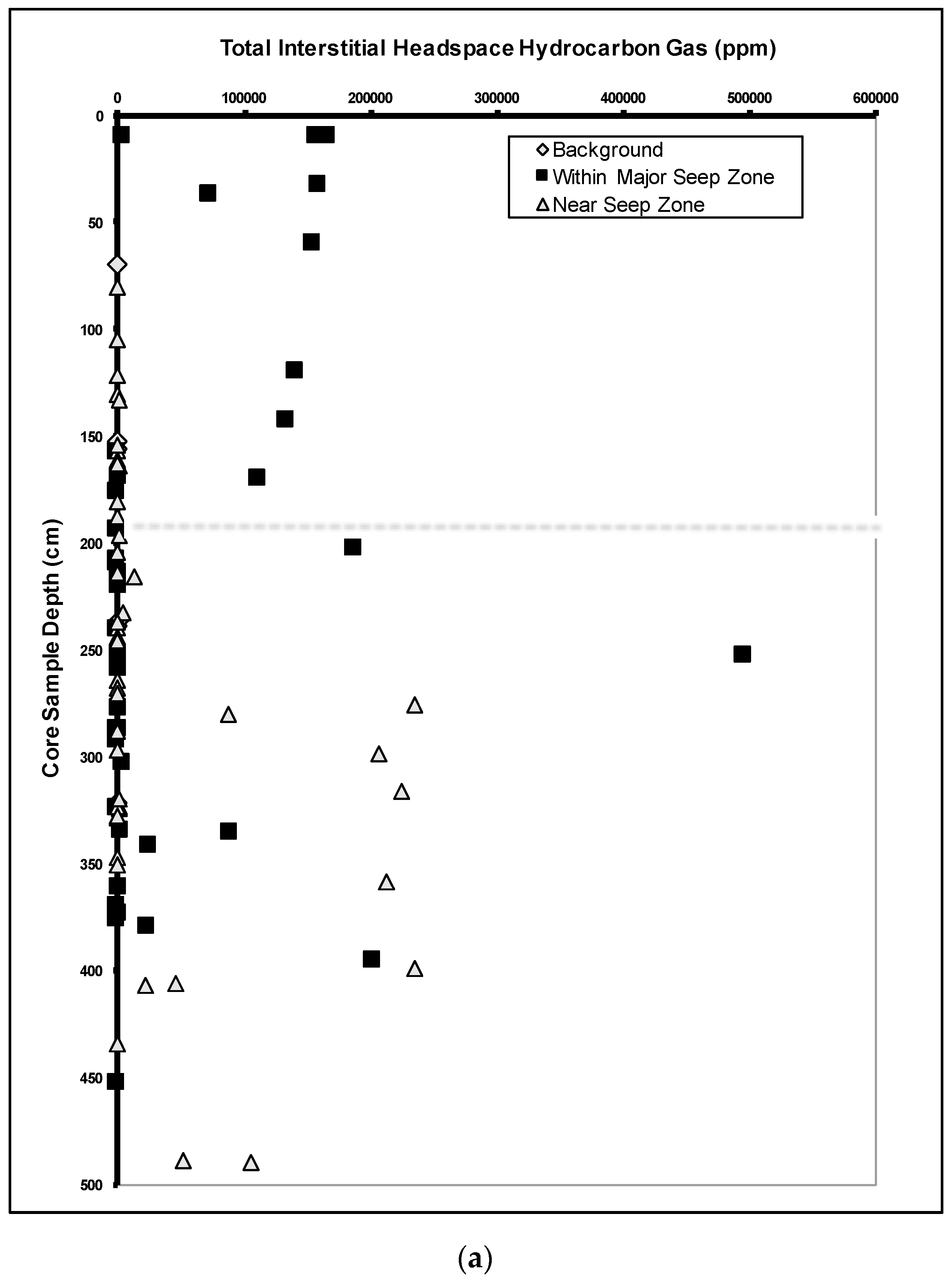

Figure 3.
Hydrocarbon gas composition interpretation chart: Total interstitial gas concentrations (ppm) versus wet gas fraction.
Figure 3.
Hydrocarbon gas composition interpretation chart: Total interstitial gas concentrations (ppm) versus wet gas fraction.

Figure 4.
Total interstitial headspace hydrocarbon gas concentrations (ppm) versus Wet Gas Fraction (∑C2–C5/∑C1–C5): (a) Offshore Gulf of Mexico with active seepage based on seismic and high molecular weight hydrocarbon analysis. Three groups of samples: Group 1 (Background) low concentration and low wet gas fraction; Group 2 (Fractionated) low concentration and enhanced wet gas fraction; and Group 3 (Anomalous) elevated concentrations with highly variable wet gas fraction. Anomalous samples in Group 3 with elevated wet gas fraction indicate thermogenic hydrocarbon seepage is present; (b) Offshore Australia with no geophysical or other geochemical evidence of seepage. Three group of samples: Group 1 (Background) low concentration and low wet gas fraction; Group 2 (Fractionated) low concentration and enhanced wet gas fraction; and Group 3 (Anomalous) elevated concentrations with low wet gas fraction. Anomalous samples in Group 3 with low wet gas fraction indicate seepage of microbial gas is present; (c) Offshore Australia with no geophysical or other geochemical evidence of seepage. No Group 1 (Background) or Group 3 (Anomalous) samples. Only low concentration samples with elevated wet gas fraction (Group 2). The Group 2 (Fractionated) samples indicate no seepage is present.
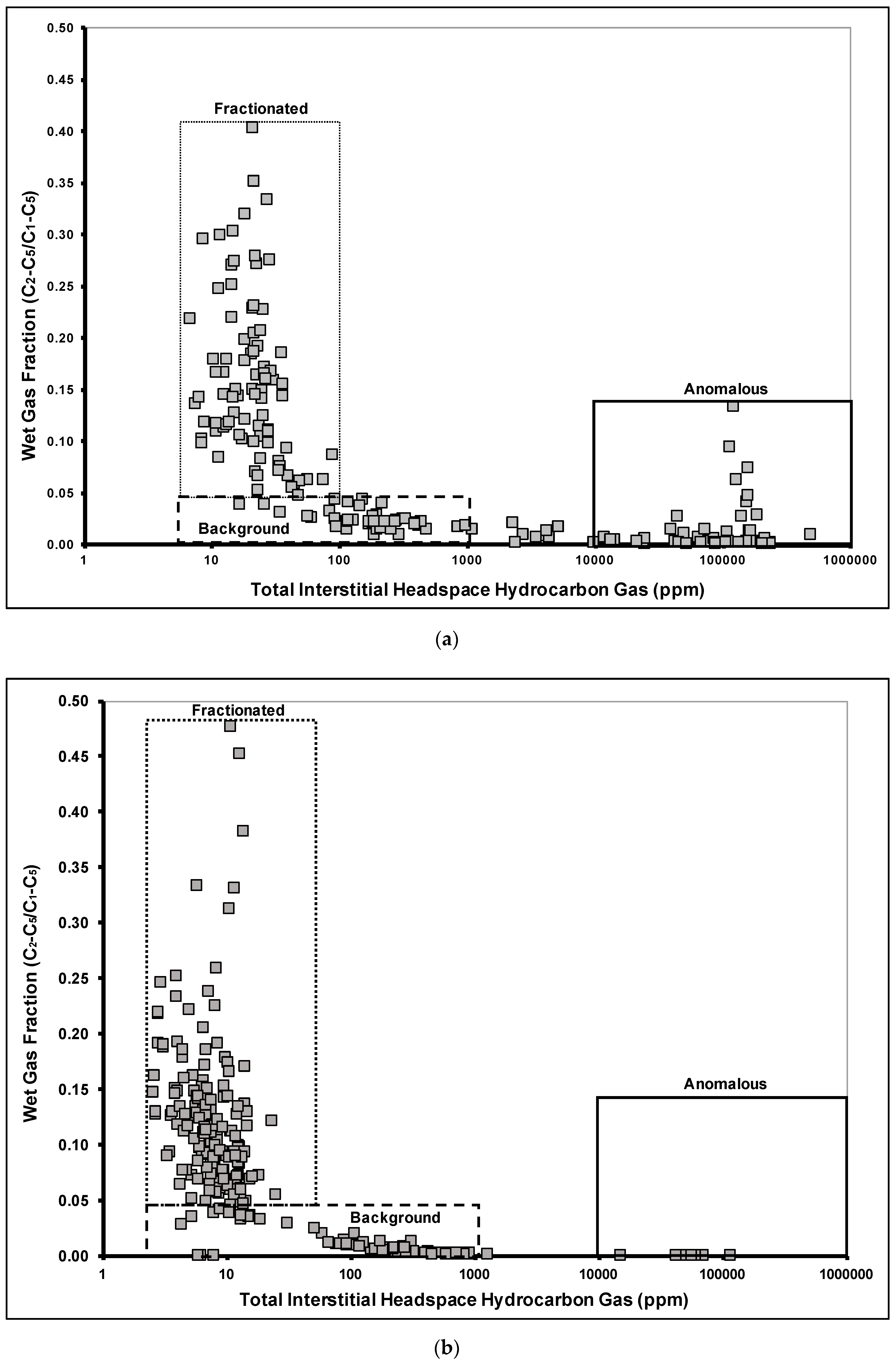

Figure 5.
Total bound hydrocarbon gas concentrations (ppm) versus Wet Gas Fraction (∑C2–C5/∑C1–C5): (a) Offshore Gulf of Mexico samples from area of active seepage based on seismic and high molecular weight hydrocarbon analysis. Total microdesorption bound hydrocarbon gas concentrations versus Wet Gas Fraction cross plot do not display similar Background, Fractionated and Anomalous groupings as was the case with the interstitial gases from replicate samples; (b) Offshore North Sea with active seepage based on seismic and high molecular weight hydrocarbon analysis. Microdesorption bound gases do not display similar background, fractionated, and anomalous groupings as was the case with the interstitial gases (data from Faber and Stahl [57]).
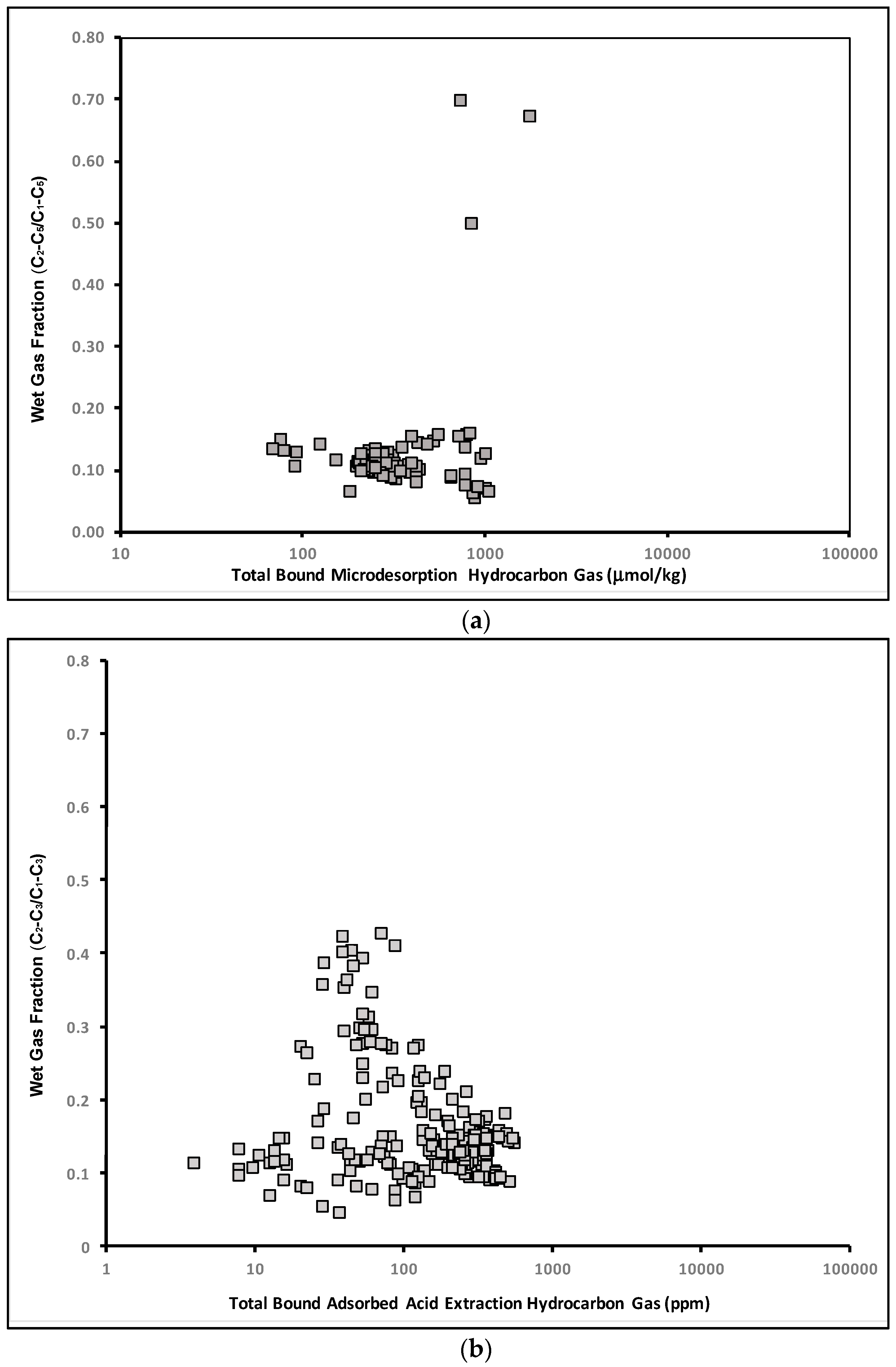
Figure 6.
Compound-specific carbon isotopic analysis interpretation chart; methane carbon isotope (δ13C1‰) versus ethane–propane separation in absolute value [(δ13C2)−(δ13C3)].
Figure 6.
Compound-specific carbon isotopic analysis interpretation chart; methane carbon isotope (δ13C1‰) versus ethane–propane separation in absolute value [(δ13C2)−(δ13C3)].

Figure 7.
Selected interstitial headspace samples with compound-specific carbon isotopic data plotted on a methane carbon isotope versus ethane–propane isotopic separation chart: (a) Offshore Gulf of Mexico interstitial headspace compound-specific isotopic dataset—microbial [35]; (b) Offshore interstitial headspace compound-specific isotopic dataset—microbial and thermogenic (data courtesy of TDI-Brooks); (c) Ethane–propane isotopic separation versus sampling depth interstitial headspace compound-specific isotopic dataset (data courtesy of TDI-Brooks).

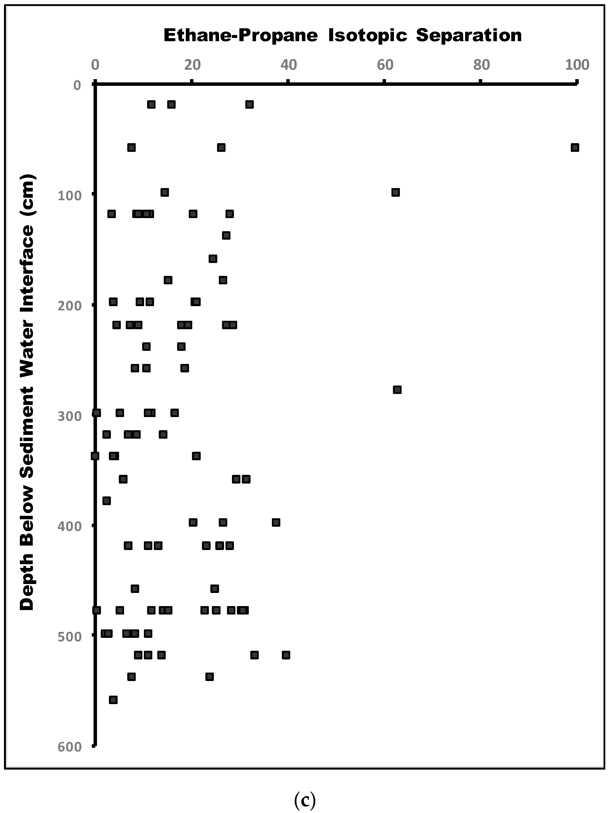
Figure 8.
Selected bound gas samples with compound-specific carbon isotopic data plotted on a methane carbon isotope versus ethane–propane isotopic separation chart: (a) Offshore Gulf of Mexico bound microdesorption compound-specific isotopic dataset—microbial [13]; (b) Offshore Gulf of Mexico bound microdesorption methane isotope versus total bound microdesorption hydrocarbon gas (μmol/kg) [13]; (c) India [61], Lapev Sea [60] and Barents Sea [62] adsorbed acid extraction compound-specific isotopic dataset—assumed to be thermogenic.


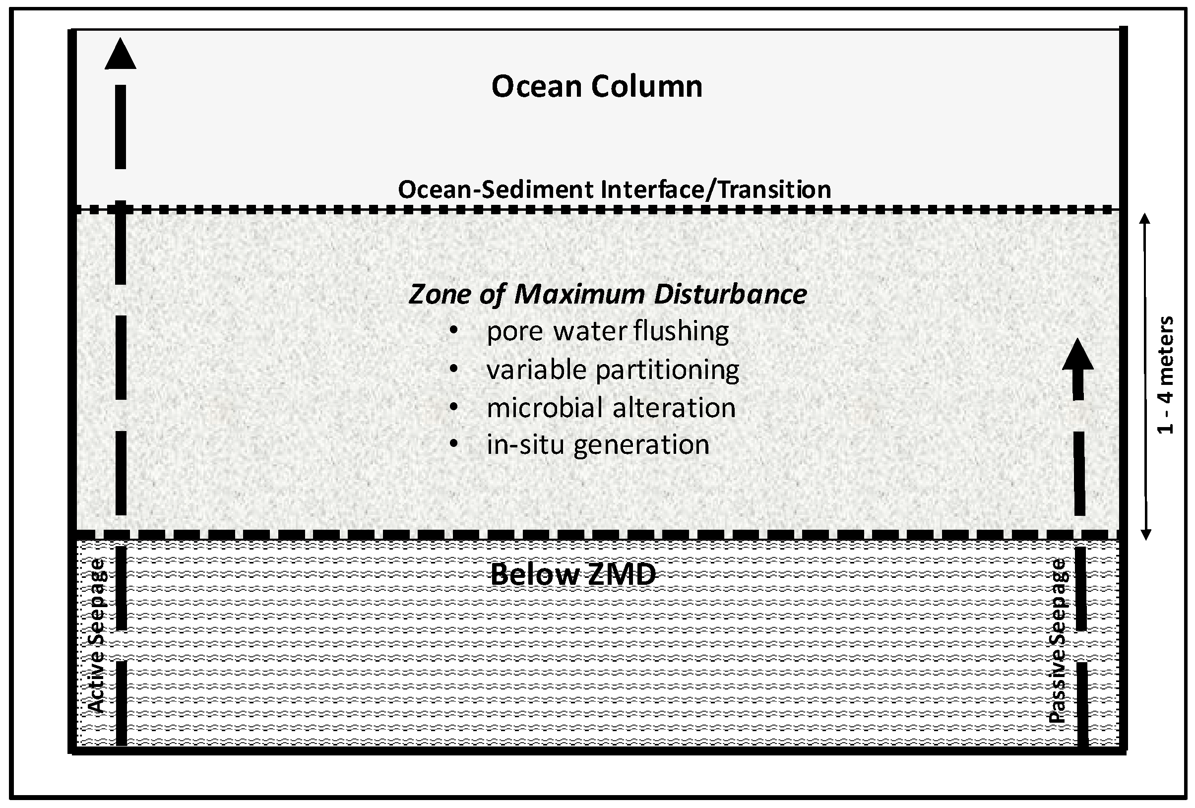
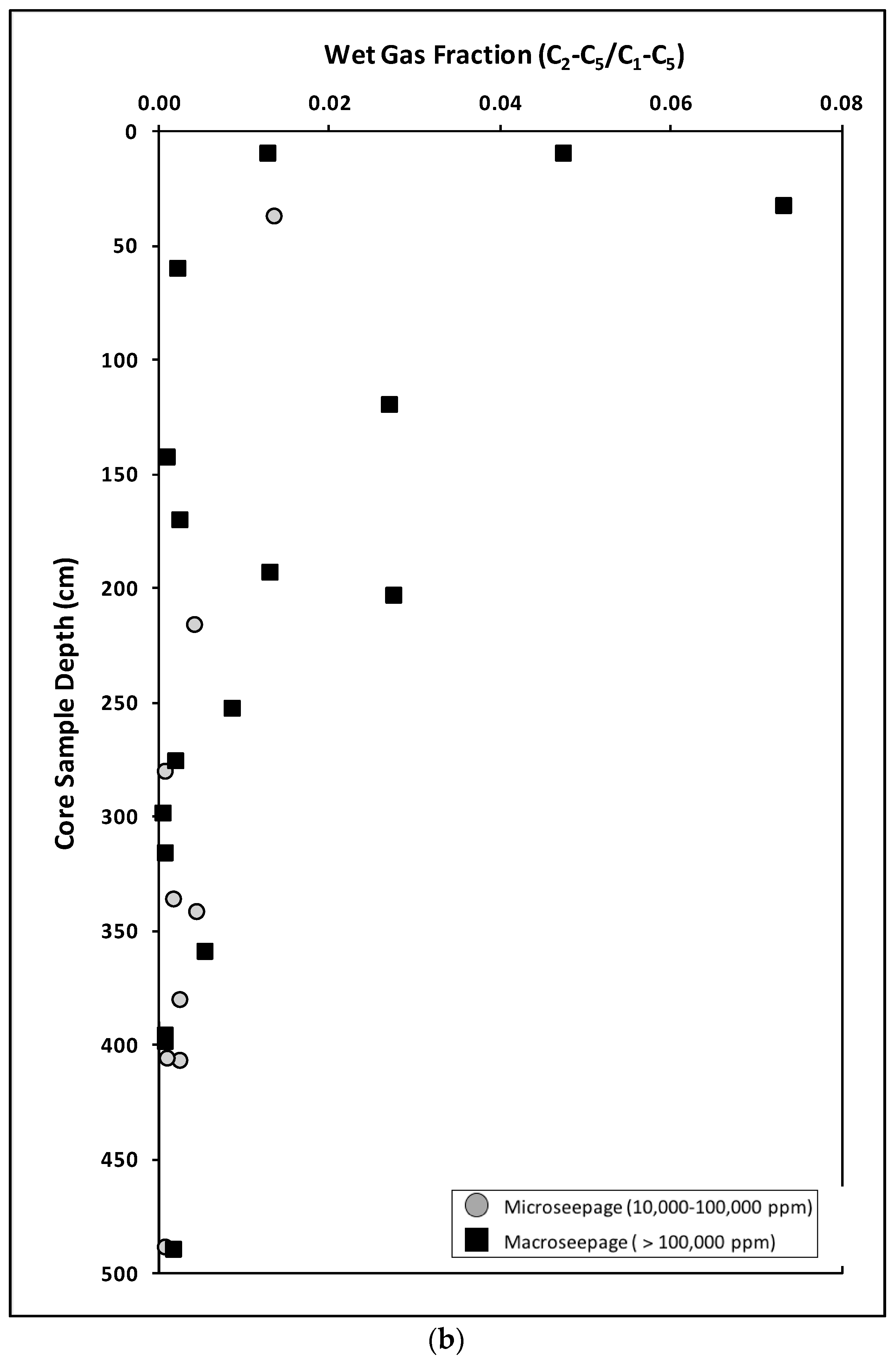
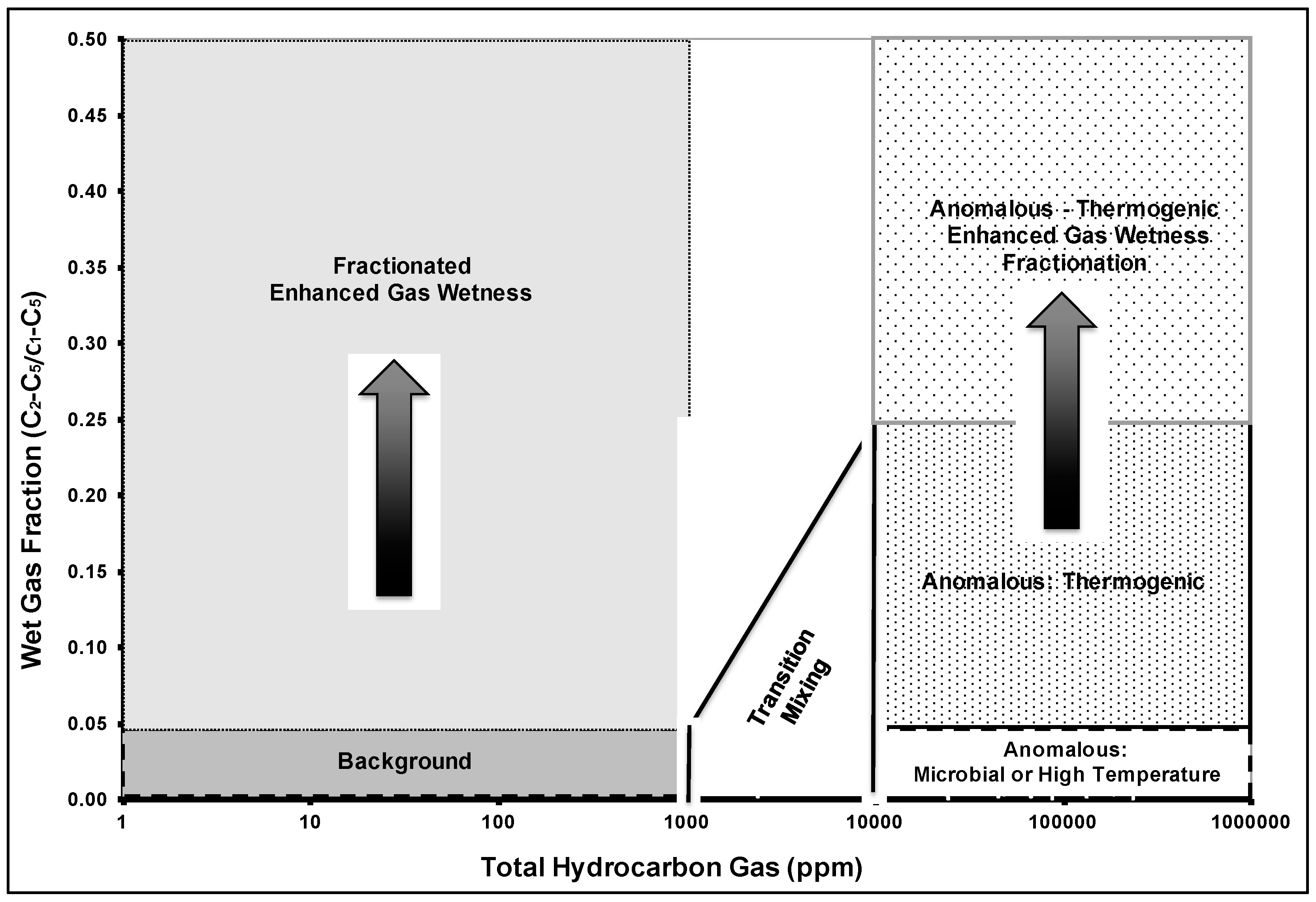
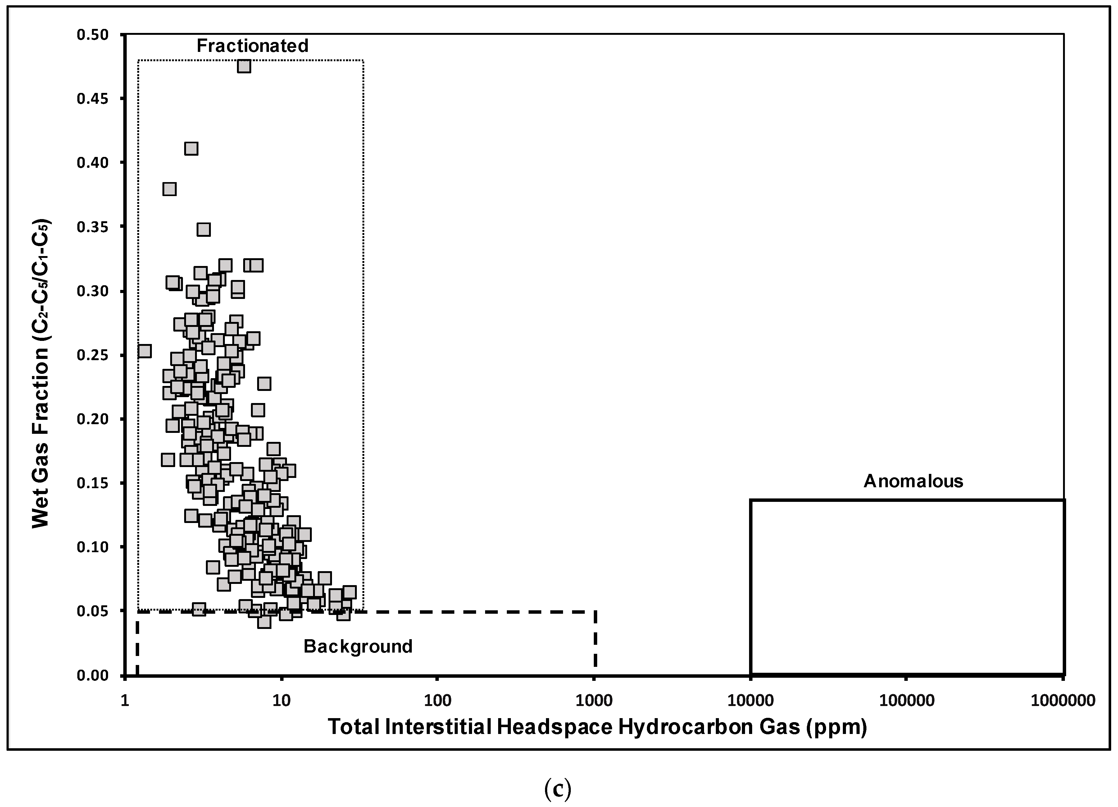
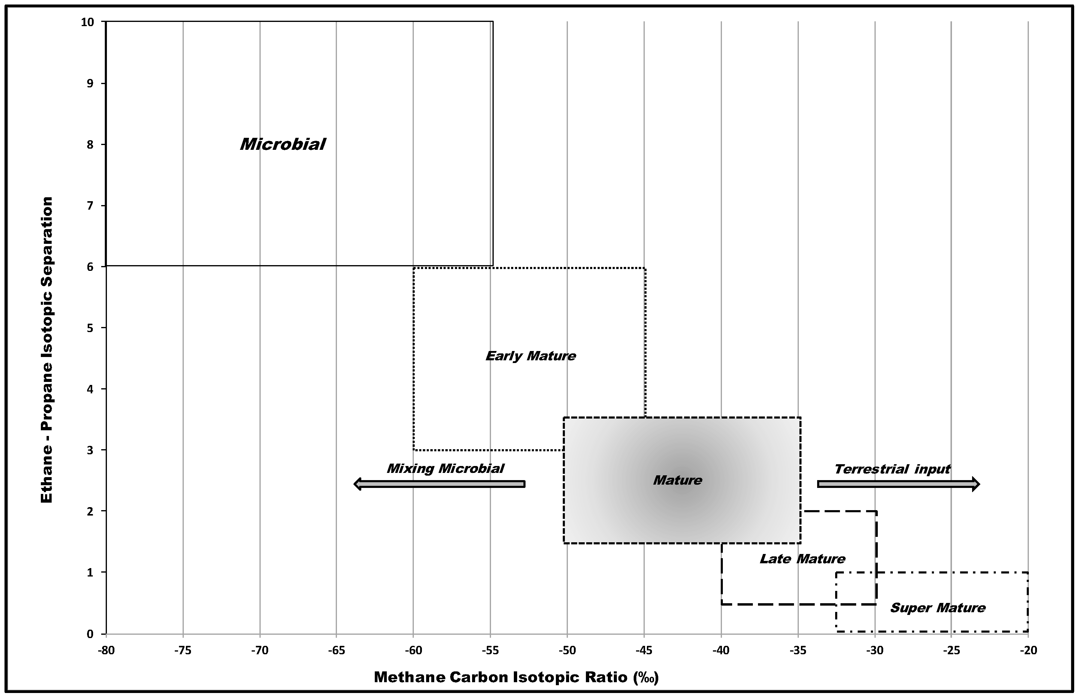
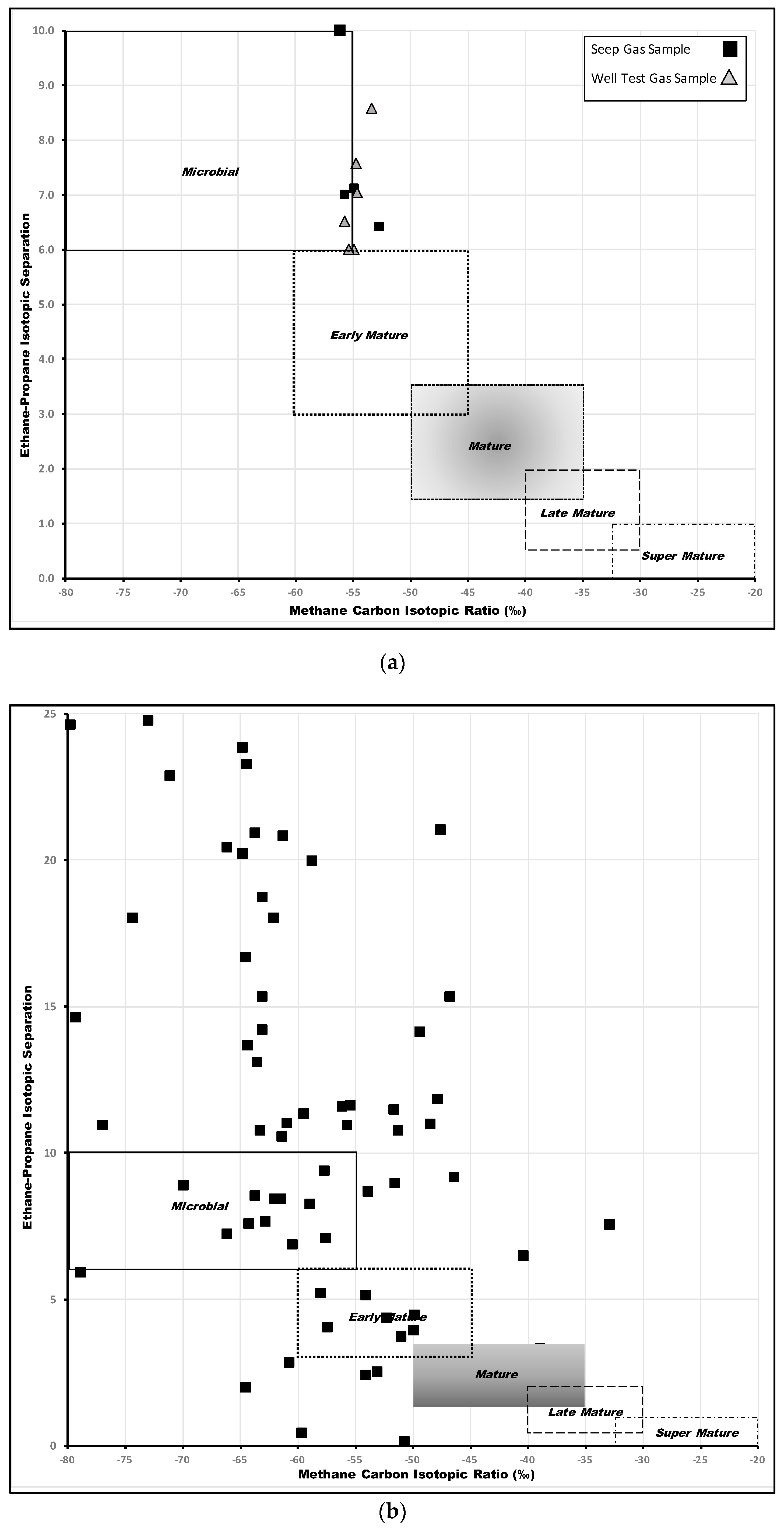
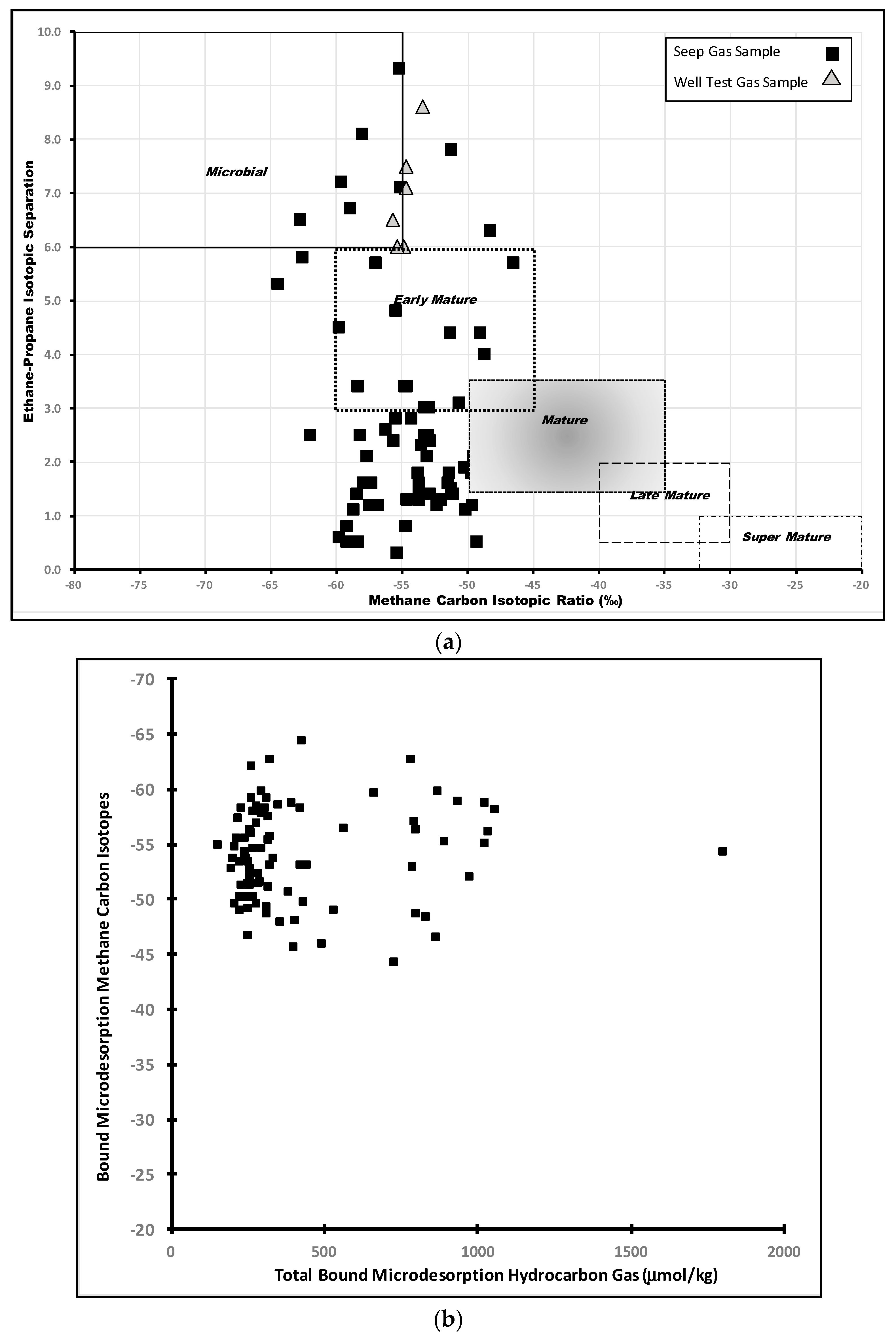
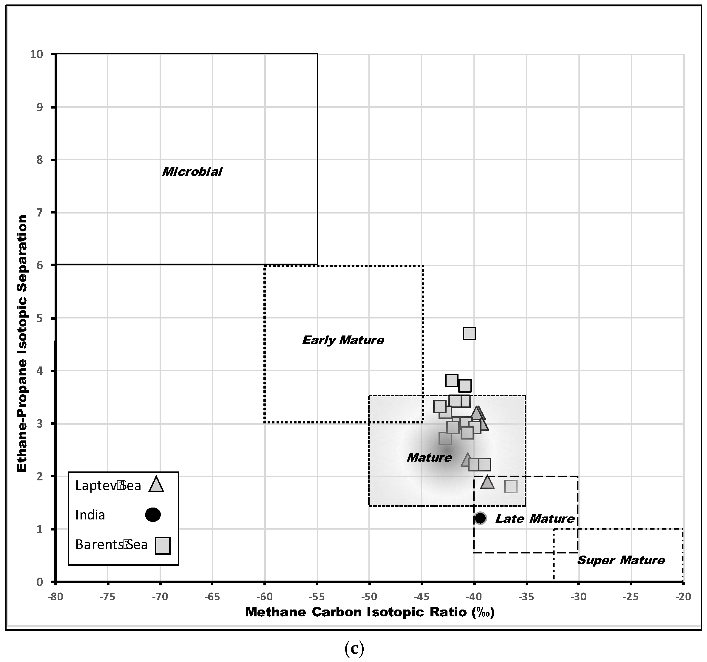
Table 1.
Ranges of bound gases reported in the literature.
| Analysis | Max | Min | Area | Reference |
|---|---|---|---|---|
| Acid extraction | 561 ppb | 208 ppb | Offshore California | [9] |
| Acid extraction | 1563 ppb | 166 ppb | U.S. Gulf of Mexico | [9] |
| Acid extraction | 562 ppb | 4 ppb | North Sea | [57] |
| Acid extraction | 1120 ppb | 160 ppb | U.S. Gulf of Mexico | [58] |
| Acid extraction | 6605 ppb | 120 ppb | Barents Sea shelf | [59] |
| Acid extraction | 461 ppb | 38 ppb | Laptev Sea | [60] |
| Acid extraction | 551 ppb | 46 ppb | Kutch Basin India | [61] |
| Acid extraction | 603 ppb | 75 ppb | Barents Sea | [62] |
| Microdesorption | 1736 nmol/g | 67 nmol/g | U.S. Gulf of Mexico | [13] |
© 2017 by the author. Licensee MDPI, Basel, Switzerland. This article is an open access article distributed under the terms and conditions of the Creative Commons Attribution (CC BY) license (http://creativecommons.org/licenses/by/4.0/).
Share and Cite
MDPI and ACS Style
Abrams, M.A. Evaluation of Near-Surface Gases in Marine Sediments to Assess Subsurface Petroleum Gas Generation and Entrapment. Geosciences 2017, 7, 35. https://doi.org/10.3390/geosciences7020035
AMA Style
Abrams MA. Evaluation of Near-Surface Gases in Marine Sediments to Assess Subsurface Petroleum Gas Generation and Entrapment. Geosciences. 2017; 7(2):35. https://doi.org/10.3390/geosciences7020035
Chicago/Turabian StyleAbrams, Michael A. 2017. "Evaluation of Near-Surface Gases in Marine Sediments to Assess Subsurface Petroleum Gas Generation and Entrapment" Geosciences 7, no. 2: 35. https://doi.org/10.3390/geosciences7020035
Note that from the first issue of 2016, this journal uses article numbers instead of page numbers. See further details here.