
Fusion of Satellite Multispectral Images Based on Ground-Penetrating Radar (GPR) Data for the Investigation of Buried Concealed Archaeological Remains

 ,
, 
Abstract
:
1. Introduction
2. Aims
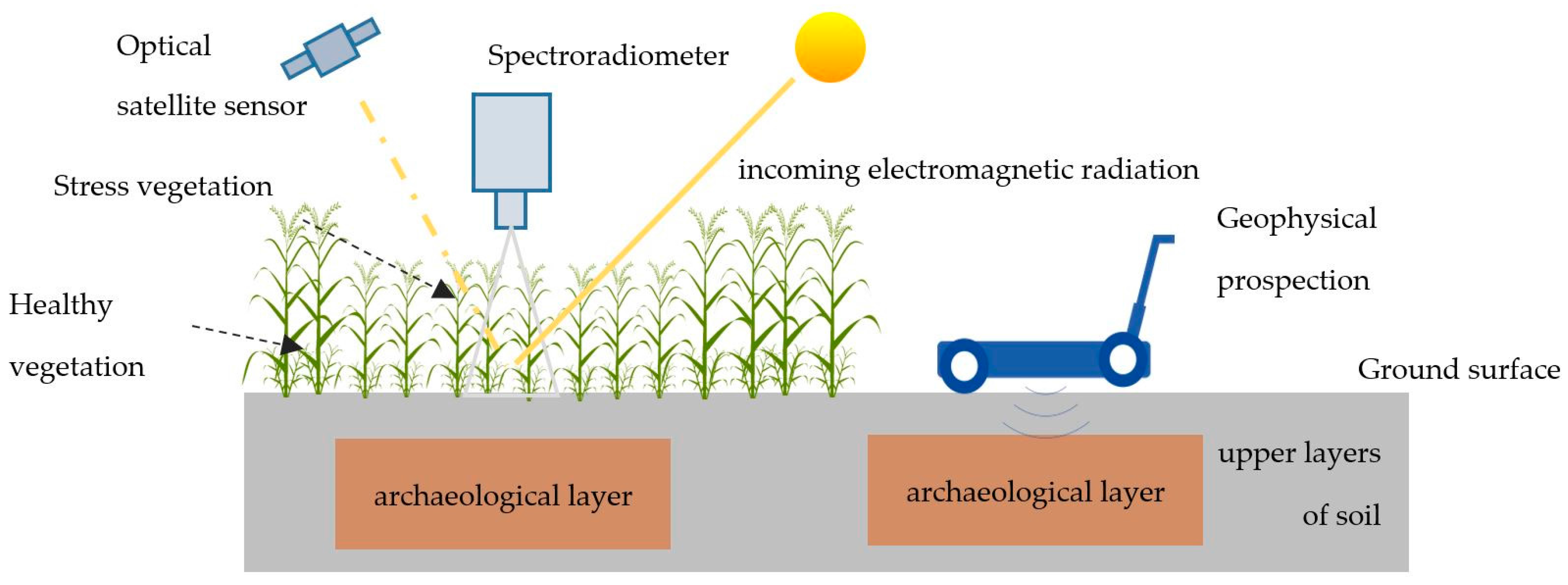
3. Methodology
4. Case Study: The Vésztő-Mágor Tell
5. Results
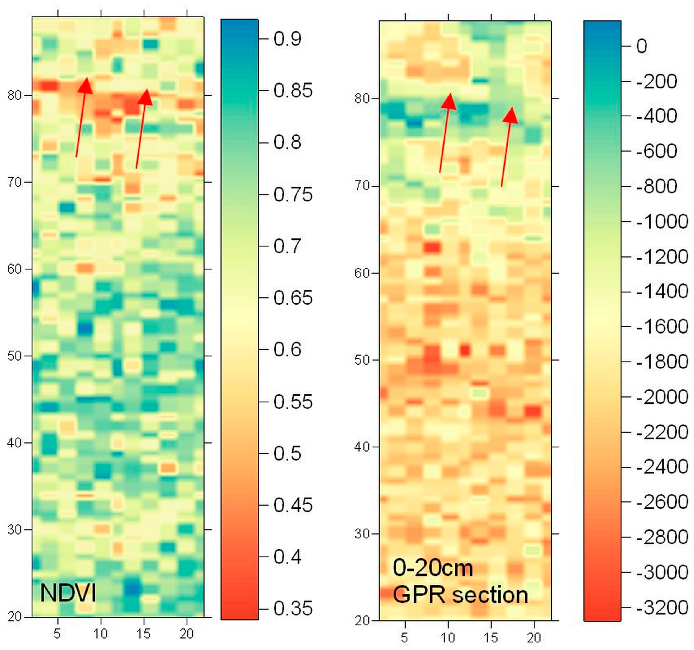
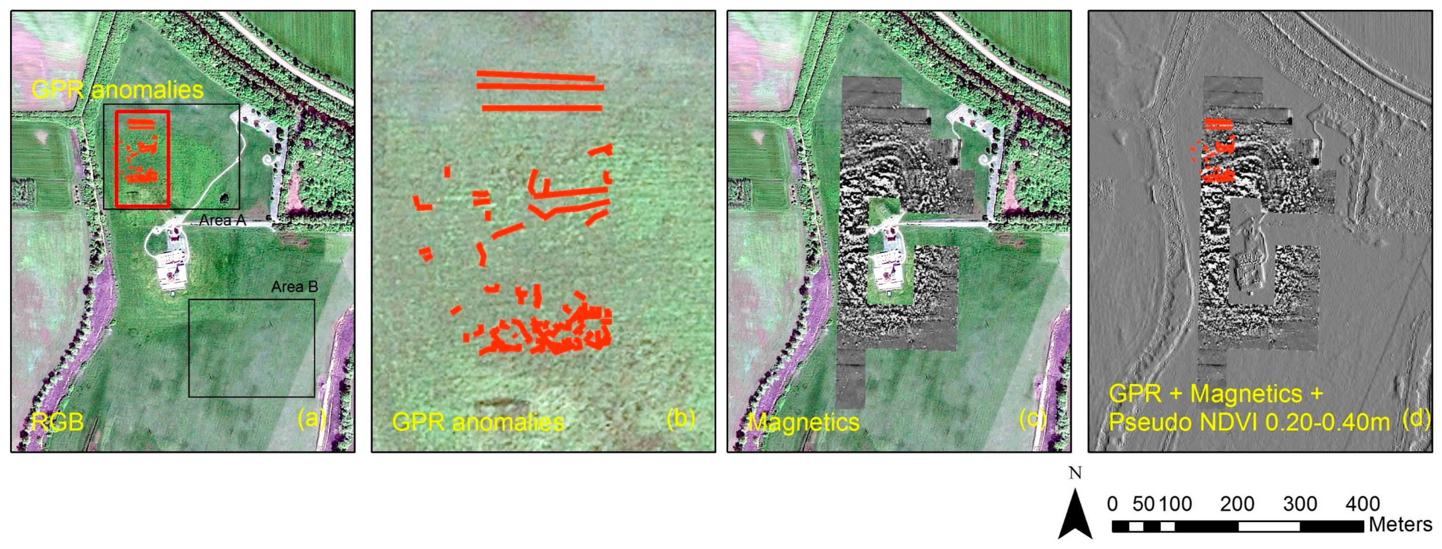
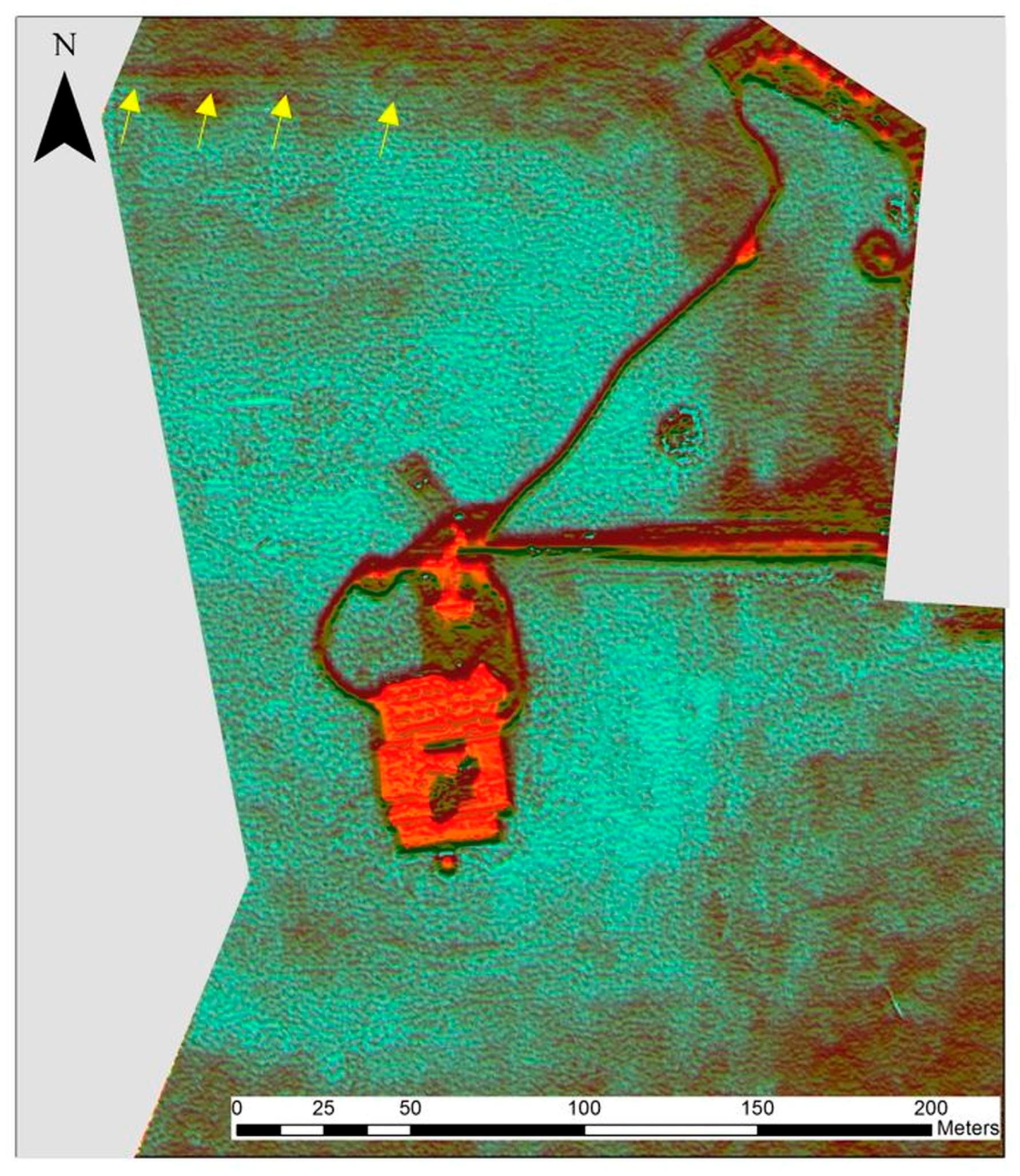
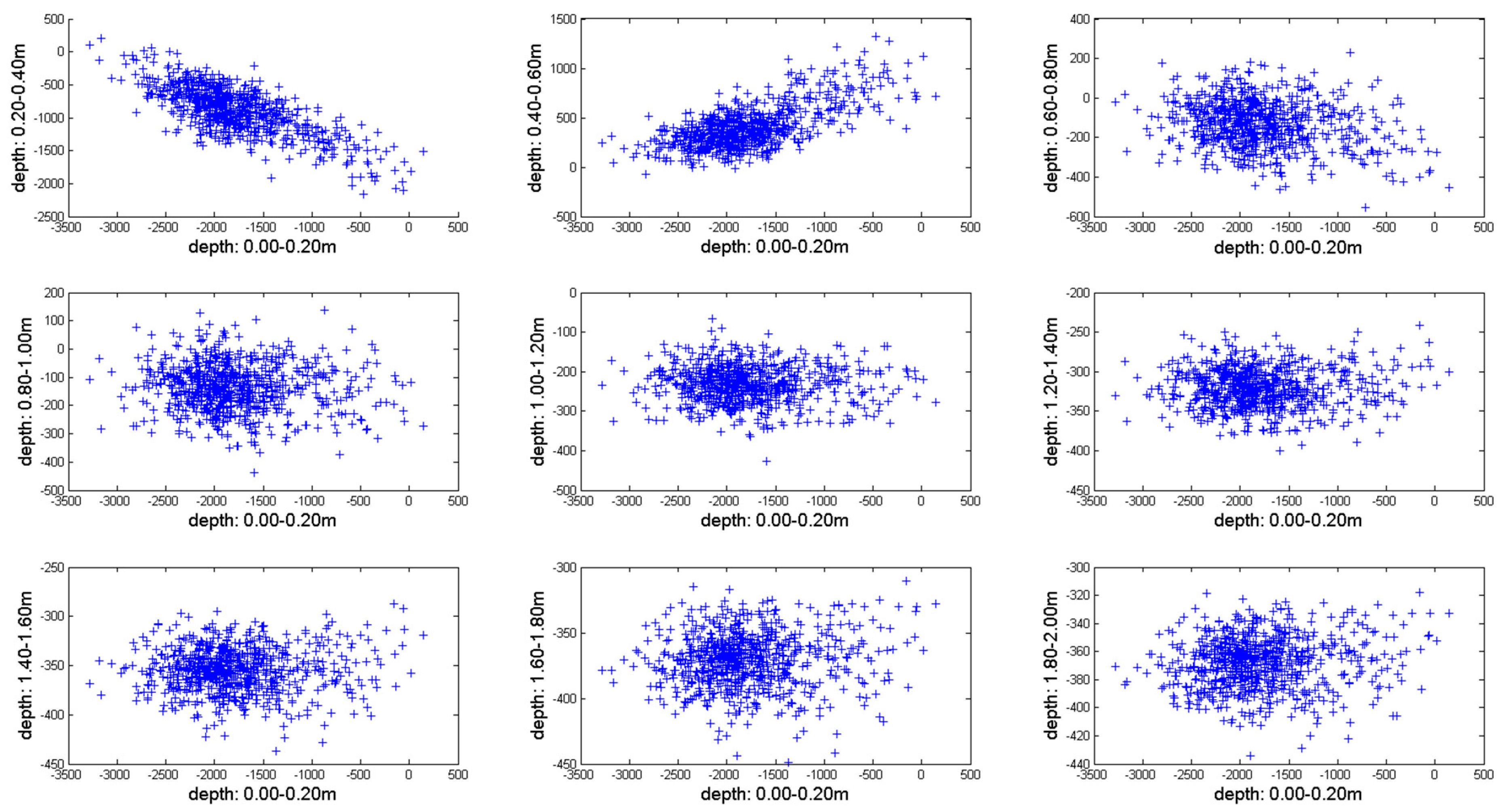
5.1. Results from GPR and Spectroradiometer
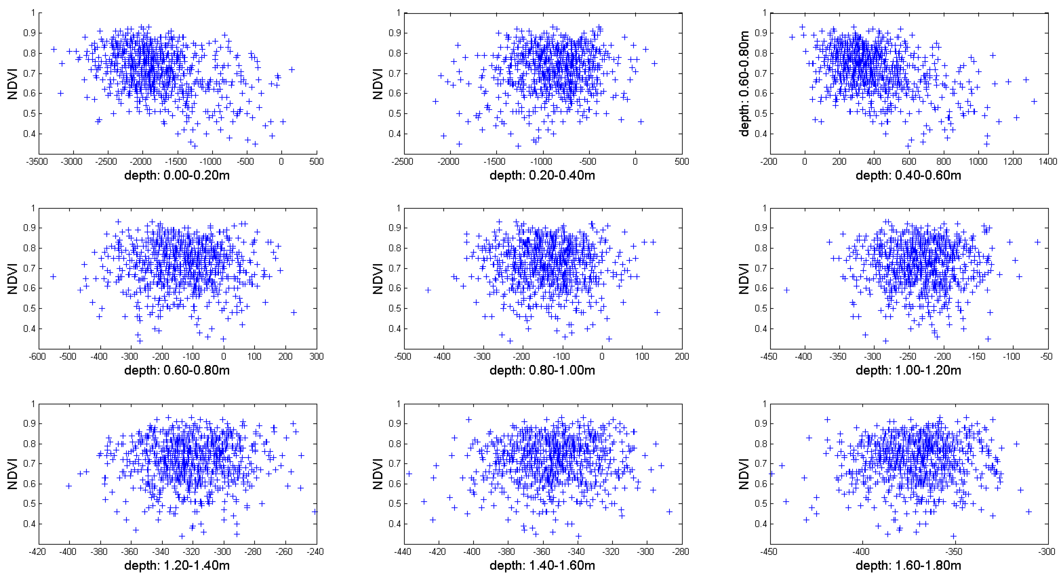
5.2. Setting up the Local Regression Model for the Enchacement of the Optical Data
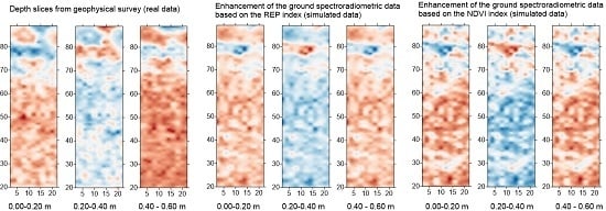
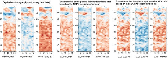
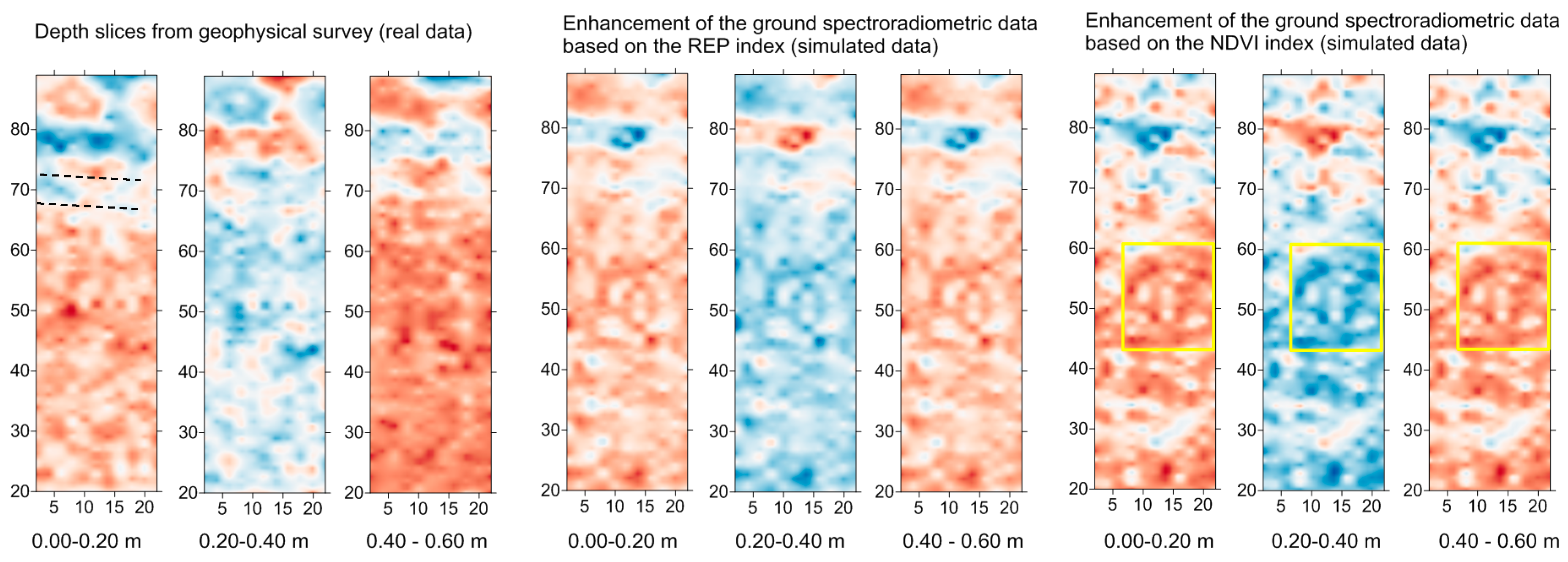
5.3. Comparison of the Fusion Model from the Spectroradiometric Measurements with the GPR Results
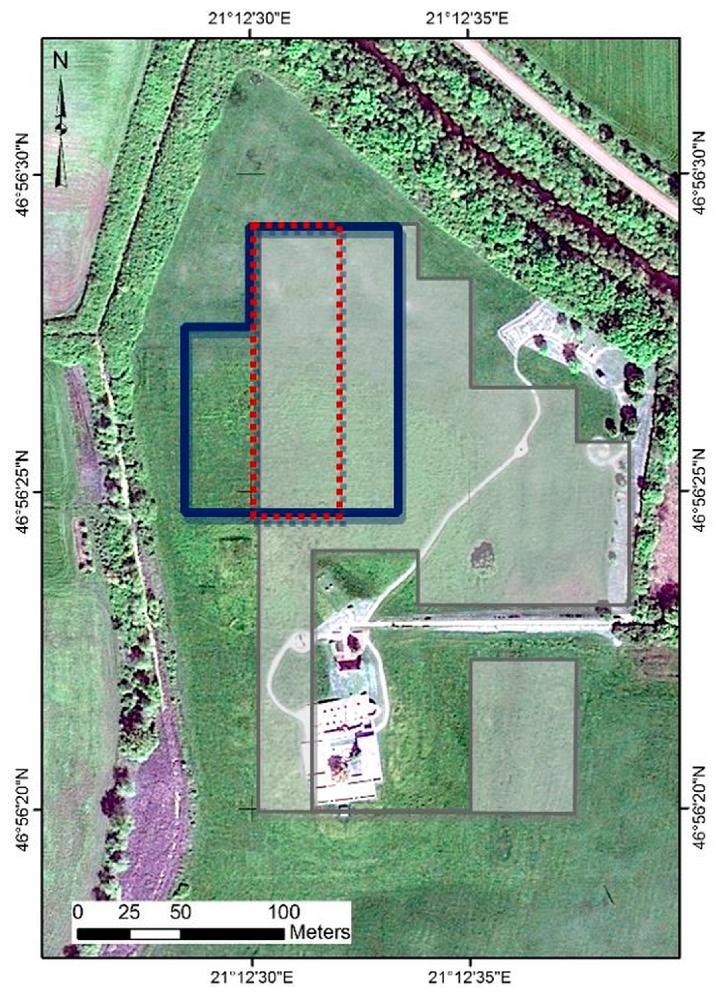
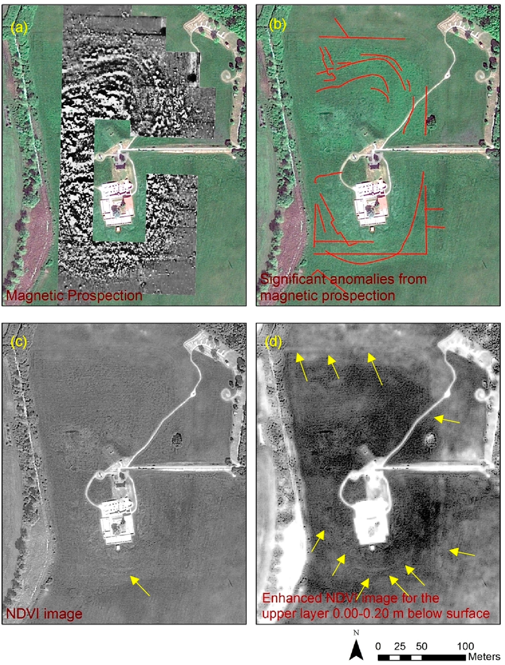
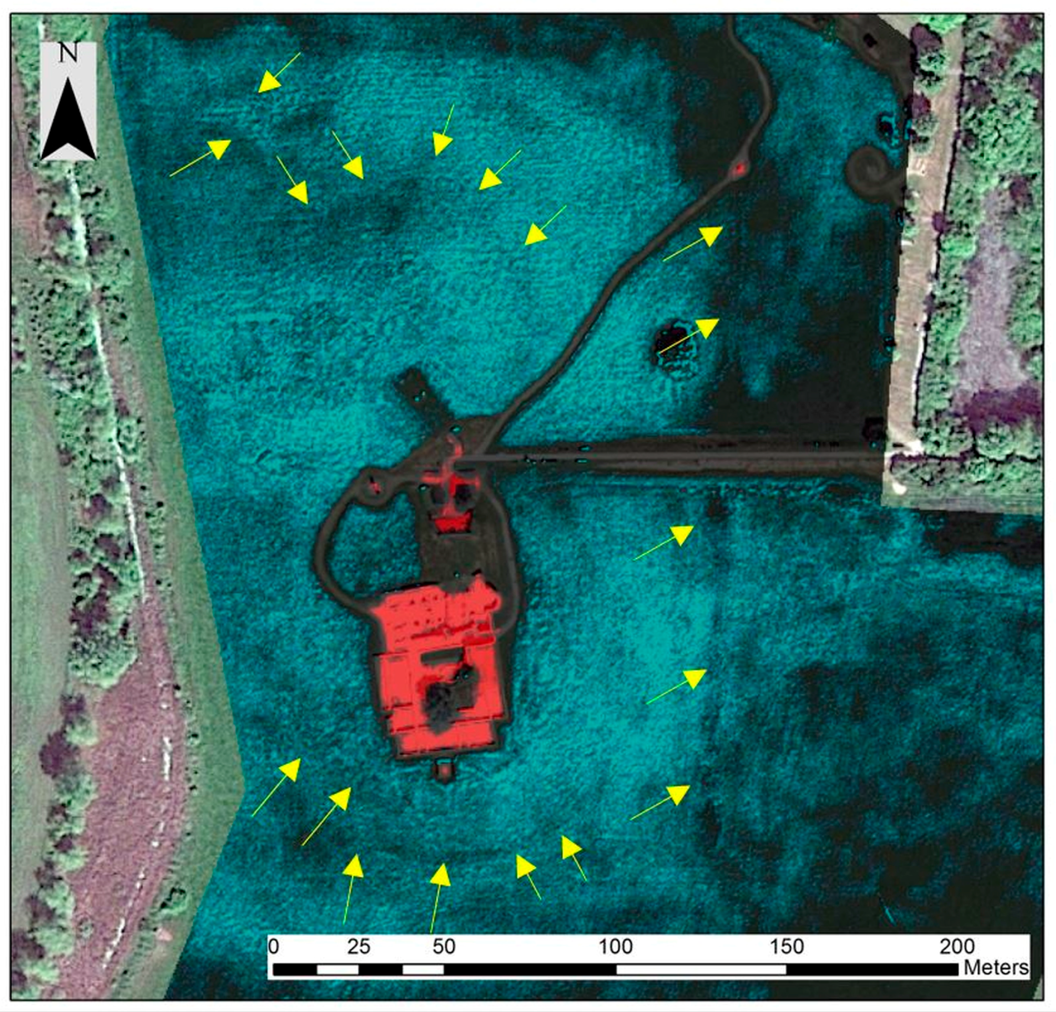
5.4. Application to the Vésztő-Mágor Tell Case Study
6. Discussion
7. Conclusions
Supplementary Materials
Acknowledgments
Author Contributions
Conflicts of Interest
References
- Lasaponara, R.; Masini, N. Satellite remote sensing in archaeology: Past, present and future perspectives. J. Archaeol. Sci. 2011, 38, 1995–2002. [Google Scholar] [CrossRef]
- Giardino, J.M. A history of NASA remote sensing contributions to archaeology. J. Archaeol. Sci. 2011, 38, 2003–2009. [Google Scholar] [CrossRef]
- Agapiou, Α.; Lysandrou, V. Remote sensing archaeology: Tracking and mapping evolution in European scientific literature from 1999 to 2015. J. Archaeol. Sci. Rep. 2015, 4, 192–200. [Google Scholar] [CrossRef]
- Keay, J.S.; Parcak, H.S.; Strutt, D.K. High resolution space and ground-based remote sensing and implications for landscape archaeology: The case from Portus, Italy. J. Archaeol. Sci. 2014, 52, 277–292. [Google Scholar] [CrossRef]
- Reinhold, S.; Belinskiy, A.; Korobov, D. Caucasia top-down: Remote sensing data for survey in a high altitude mountain landscape. Quat. Int. 2016, 402, 46–60. [Google Scholar] [CrossRef]
- Barone, M.P.; Desibio, L. A remote sensing approach to understanding the archaeological potential: the case study of some Roman evidence in Umbria (Italy). Int. J. Archaeol. 2015, 3, 37–44. [Google Scholar] [CrossRef]
- Barone, M.P.; Desibio, L. Landscape archaeology of southern Umbria (Italy) using the GPR technique. In Proceedings of the 2015 8th International Workshop on Advanced Ground Penetrating Radar (IWAGPR), Florence, Italy, 7–10 July 2015. [Google Scholar]
- Alexakis, D.; Sarris, A.; Astaras, T.; Albanakis, Κ. Detection of neolithic settlements in thessaly (Greece) through multispectral and hyperspectral satellite imagery. Sensors 2009, 9, 1167–1187. [Google Scholar] [CrossRef] [PubMed]
- Alexakis, A.; Sarris, A.; Astaras, T.; Albanakis, K. Integrated GIS, remote sensing and geomorphologic approaches for the reconstruction of the landscape habitation of Thessaly during the Neolithic period. J. Archaeol. Sci. 2011, 38, 89–100. [Google Scholar] [CrossRef]
- Banerjee, R.; Srivastava, K.P. Reconstruction of contested landscape: Detecting land cover transformation hosting cultural heritage sites from Central India using remote sensing. Land Use Policy 2013, 34, 193–203. [Google Scholar] [CrossRef]
- Agapiou, A.; Alexakis, D.D.; Lysandrou, V.; Sarris, A.; Cuca, B.; Themistocleous, K.; Hadjimitsis, D.G. Impact of Urban Sprawl to archaeological research: the case study of Paphos area in Cyprus. J. Cult. Herit. 2015, 16, 671–680. [Google Scholar] [CrossRef]
- Cerra, D.; Plank, S.; Lysandrou, V.; Tian, J. Cultural Heritage Sites in Danger—Towards Automatic Damage Detection from Space. Remote Sens. 2016, 8, 781. [Google Scholar] [CrossRef]
- Chen, F.; Lasaponara, R.; Masini, N. An Overview of Satellite Synthetic Aperture Radar Remote Sensing in Archaeology: From Site Detection to Monitoring. J. Cult. Herit. 2017, 23, 5–11. [Google Scholar] [CrossRef]
- Stek, D.T. Drones over Mediterranean landscapes. The potential of small UAV's (drones) for site detection and heritage management in archaeological survey projects: A case study from Le Pianelle in the Tappino Valley, Molise (Italy). J. Cult. Herit. 2016, 22, 1066–1071. [Google Scholar] [CrossRef]
- Siart, C.; Eitel, B.; Panagiotopoulos, D. Investigation of past archaeological landscapes using remote sensing and GIS: a multi-method case study from Mount Ida, Crete. J. Archaeol. Sci. 2008, 35, 2918–2926. [Google Scholar] [CrossRef]
- Sarris, A.; Papadopoulos, N.; Agapiou, A.; Salvi, M.C.; Hadjimitsis, D.G.; Parkinson, A.; Yerkes, R.W.; Gyucha, A.; Duffy, R.P. Integration of geophysical surveys, ground hyperspectral measurements, aerial and satellite imagery for archaeological prospection of prehistoric sites: The case study of Vésztő-Mágor Tell, Hungary. J. Archaeol. Sci. 2013, 40, 1454–1470. [Google Scholar] [CrossRef]
- Malfitana, D.; Leucci, G.; Fragalà, G.; Masini, N.; Scardozzi, G.; Cacciaguerra, G.; Santagati, C.; Shehi, E. The potential of integrated GPR survey and aerial photographic analysis of historic urban areas: A case study and digital reconstruction of a Late Roman villa in Durrës (Albania). J. Archaeol. Sci. Rep. 2015, 4, 276–284. [Google Scholar] [CrossRef]
- Morehart, C.T. Mapping ancient chinampa landscapes in the Basin of Mexico: A remote sensing and GIS approach. J. Archaeol. Sci. 2012, 39, 2541–2551. [Google Scholar] [CrossRef]
- Traviglia, A.; Cottica, D. Remote sensing applications and archaeological research in the Northern Lagoon of Venice: the case of the lost settlement of Constanciacus. J. Archaeol. Sci. 2011, 38, 2040–2050. [Google Scholar] [CrossRef]
- Gallo, D.; Ciminale, M.; Becker, H.; Masini, N. Remote sensing techniques for reconstructing a vast Neolithic settlement in Southern Italy. J. Archaeol. Sci. 2009, 36, 43–50. [Google Scholar] [CrossRef]
- Keay, S.; Earl, G.; Hay, S.; Kay, S.; Ogden, J.; Strutt, K.D. The role of integrated survey methods in the assessment of archaeological landscapes: the case of Portus. Archaeol. Prospect. 2009, 15, 154–166. [Google Scholar] [CrossRef]
- Ciminale, M.; Gallo, D.; Lasaponara, R.; Masini, N. A multiscale approach for reconstructing archaeological landscapes: Applications in northern Apulia (Italy). Archaeol. Prospect. 2009, 16, 143–153. [Google Scholar] [CrossRef]
- Piro, S.; Mauriello, P.; Cammarano, F. Quantitative integration of geophysical methods for archaeological prospection. Archaeol. Prospect. 2000, 7, 203–213. [Google Scholar] [CrossRef]
- Kvamme, K.L. Integrating Multidimensional Geophysical Data. Archaeol. Prospect. 2006, 13, 57–72. [Google Scholar] [CrossRef]
- Kvamme, K.; Ernenwein, E.; Hargrave, M.; Sever, T.; Harmon, D.; Limp, F. New Approaches to the Use and Integration of Multi-Sensor Remote Sensing for Historic Resource. Identification and Evaluation, Report of SERDP Project, SI-1263, University of Arkansas, Center for Advanced Spatial Technologies. 10 November 2006. Available online: http://s3.amazonaws.com/academia.edu.documents/10387950/si-1263-part1.pdf?AWSAccessKeyId=AKIAIWOWYYGZ2Y53UL3A&Expires=1496724950&Signature=BKPfKdlCCLxJ9Q%2BoU30JtrM3MP8%3D&response-content-disposition=inline%3B%20filename%3DNew_Approaches_to_the_Use_and_Integratio.pdf (accessed on 6 June 2017).
- Aiazzi, B.; Baronti, S.; Lotti, F.; Selva, M. A comparison between global and context-adaptive pansharpening of multispectral images. IEEE Geosci. Remote Sens. Lett. 2009, 6, 302–306. [Google Scholar] [CrossRef]
- Garzelli, A. Pansharpening of Multispectral Images Based on Nonlocal Parameter Optimization. IEEE Trans. Geosci. Remote Sens. 2015, 53, 2096–2107. [Google Scholar] [CrossRef]
- Agapiou, A.; Alexakis, D.D.; Sarris, A.; Hadjimitsis, D.G. Colour to grayscale pixels: Re-seeing grayscale archived aerial photographs and declassified satellite CORONA images based on image fusion techniques. Archaeol. Prospect. 2016, 23, 231–241. [Google Scholar] [CrossRef]
- Schaepman, E.M.; Ustin, L.S.; Plaza, J.A.; Painter, H.T.; Verrelst, J.; Liang, S. Earth system science related imaging spectroscopy—An assessment. Remote Sens. Environ. 2009, 113, S123–S137. [Google Scholar] [CrossRef]
- Agapiou, A.; Alexakis, D.D.; Sarris, A.; Hadjimitsis, D.G. Evaluating the potentials of Sentinel-2 for archaeological perspective. Remote Sens. 2014, 6, 2176–2194. [Google Scholar] [CrossRef]
- Agapiou, A.; Sarris, A.; Papadopoulos, N.; Alexakis, D.D.; Hadjimitsis, D.G. 3D pseudo GPR sections based on NDVI values: Fusion of optical and active remote sensing techniques at the Vészto-Mágor tell, Hungary. In Archaeological Research in the Digital Age, Proceedings of the 1st Conference on Computer Applications and Quantitative Methods in Archaeology Greek Chapter (CAA-GR), Rethymno Crete, Greece, 6–8 March 2014; Papadopoulos, C., Paliou, E., Chrysanthi, A., Kotoula, E., Sarris, A., Eds.; Institute for Mediterranean Studies-Foundation of Research and Technology (IMS-Forth): Rethymno, Greece, 2015. [Google Scholar]
- Agapiou, A.; Hadjimitsis, D.G.; Alexakis, D.D. Evaluation of broadband and narrowband vegetation indices for the identification of archaeological crop marks. Remote Sens. 2012, 4, 3892–3919. [Google Scholar] [CrossRef]
- Hegedűs, K. Vésztő-Mágori-domb. In Magyarország Régészeti Topográfiája VI. Békés Megye Régészeti Topográfiája: A Szeghalmi Járás 1982 IV/1; Ecsedy, I., Kovács, L., Maráz, B., Torma, I., Eds.; Akadémiai Kiadó: Budapest, Hungary, 1982; pp. 184–185. (In Hungarian) [Google Scholar]
- Hegedűs, K.; Makkay, J. Vésztő-Mágor: A Settlement of the Tisza Culture. In The Late Neolithic of the Tisza Region: A Survey of Recent Excavations and their Findings; Tálas, L., Raczky, P, Eds.; Szolnok County Museums: Budapest-Szolnok, Hungary, 1987; pp. 85–104. [Google Scholar]
- Makkay, J. Vésztő–Mágor. Ásatás a szülőföldön. Békés Megyei Múzeumok Igazgatósága, Békéscsaba. 2004. Available online: http://mek.oszk.hu/07600/07616/07616.pdf (accessed on 6 June 2017).
- Parkinson, W.A. Tribal boundaries: Stylistic variability and social boundary maintenance during the transition to the Copper Age on the Great Hungarian Plain. J. Anthropol. Archaeol. 2006, 25, 33–58. [Google Scholar] [CrossRef]
- Juhász, I. A Csolt nemzetség monostora. In A középkori Dél-Alföld és Szer; Kollár, T., Ed.; pp. 281–304. Available online: http://opac.regesta-imperii.de/lang_en/anzeige.php?sammelwerk=A+k%C3%B6z%C3%A9pkori+D%C3%A9l-Alf%C3%B6ld+%C3%A9s+Szer (accessed on 6 June 2017).
- Gyucha, A.; Yerkes, W.R.; Parkinson, A.W.; Sarris, A.; Papadopoulos, N.; Duffy, R.P.; Salisbury, B.R. Settlement Nucleation in the Neolithic: A Preliminary Report of the Körös Regional Archaeological Project’s Investigations at Szeghalom-Kovácshalom and Vésztő-Mágor. In Neolithic and Copper Age between the Carpathians and the Aegean Sea: Chronologies and Technologies from the 6th to the 4th Millennium BCE. International Workshop Budapest 2012; Hansen, S., Raczky, P., Anders, A., Reingruber, A., Eds.; Habelt-Verlag: Bonn, Germany, 2015; pp. 129–142. [Google Scholar]


| Characteristics | Satellite Remote Sensing (for Optical High Resolution) | Ground-Penetrating Radar | Ground Spectroscopy |
|---|---|---|---|
| Spatial resolution | Medium–High | High–Very High (adjustable) | High–Very High (adjustable) |
| Spectral range | Visible-Near Infrared (Multispectral) | Microwave | Vis-NIR (Hyperspectral) |
| Spatial extent | Several km2 | Several Hectares | Several m2 |
| 3D visualization | No | Yes | No |
| Soil penetration | No | Yes | No |
| Archive data | Yes | No | No |
| Type of information | Raster | Point | Raster |
| Slice (in m Below Surface) | R Value |
|---|---|
| 0.20–0.40 | −0.74 |
| 0.40–0.60 | 0.67 |
| 0.60–0.80 | −0.22 |
| 0.80–1.00 | −0.07 |
| 1.00–1.20 | −0.04 |
| 1.20–1.40 | −0.01 |
| 1.40–1.60 | 0.03 |
| 1.60–1.80 | 0.06 |
| 1.80–2.00 | 0.10 |
| Slice (in m Below Surface) | R Value |
|---|---|
| 0.00–0.20 | −0.35 |
| 0.20–0.40 | 0.12 |
| 0.40–0.60 | −0.39 |
| 0.60–0.80 | −0.01 |
| 0.80–1.00 | −0.03 |
| 1.00–1.20 | 0.01 |
| 1.20–1.40 | 0.05 |
| 1.40–1.60 | 0.08 |
| 1.60–1.80 | 0.05 |
| No. | General Equations | Name |
|---|---|---|
| 1. | f(x) = a × x + b | Linear |
| 2. | f(x) = a × exp(b × x) | Exponential (one term) |
| 3. | f(x) = a × exp(b × x) + c × exp(d × x) | Exponential (two terms) |
| 4. | f(x) = a0 + a1 × cos(x × w) + b1 × sin(x × w) | Fourier (one term) |
| 5. | f(x) = a0 + a1 × cos(x × w) + b1 × sin(x × w) + a2 × cos(2 × x × w) + b2 × sin(2 × x × w) | Fourier (two terms) |
| 6. | f(x) = a1 × exp(−((x − b1)/c1)2 | Gaussian (one term) |
| 7 | f(x) = a1 × exp(−((x − b1)/c1)2) + a2 × exp(−((x − b2)/c2)2) | Gaussian (two terms) |
| 8. | f(x) = p1 × x2 + p2 × x + p3 | Polynomial (second order) |
| 9. | f(x) = p1 × x3 + p2 × x2 + p3 × x + p4 | Polynomial (third order) |
| 10. | f(x) = a × xb | Power (one term) |
| 11. | f(x) = a × xb + c | Power (two terms) |
| 12. | f(x) = (p1 × x + p2)/(x + q1) | Rational (first degree) |
| 13. | f(x) = (p1 × x2 + p2 × x + p3)/(x + q1) | Rational (second degree) |
| 14. | f(x) = a1 × sin(b1 × x + c1) | Sum of Sin (one term) |
| 15. | f(x) = a1 × sin(b1 × x + c1) + a2 × sin(b2 × x + c2) | Sum of Sin (two terms) |
| Depth/Index | BAND1 | BAND2 | BAND3 | BAND4 | EVI | Green NDVI | NDVI | SR | MSR | MTVI2 |
| 0.000 to 0.200 m | 0.23 | 0.15 | 0.22 | −0.33 | −0.32 | −0.41 | −0.37 | −0.29 | 0.28 | 0.32 |
| 0.200 to 0.400 m | −0.12 | −0.11 | −0.07 | 0.11 | 0.09 | 0.22 | 0.15 | 0.10 | −0.10 | −0.10 |
| 0.400 to 0.600 m | 0.26 | 0.17 | 0.27 | −0.33 | −0.38 | −0.44 | −0.41 | −0.33 | 0.32 | 0.37 |
| 0.600 to 0.800 m | 0.04 | 0.05 | 0.03 | 0.05 | 0.00 | −0.01 | 0.00 | −0.02 | 0.02 | 0.00 |
| Depth/Index | RDVI | IRG | PVI | RVI | TSAVI | MSAVI | GEMI | ARVI | SARVI | OSAVI |
| 0.000 to 0.200 m | −0.38 | 0.24 | −0.37 | 0.38 | −0.37 | −0.38 | −0.32 | −0.35 | 0.40 | −0.37 |
| 0.200 to 0.400 m | 0.14 | −0.01 | 0.12 | −0.16 | 0.15 | 0.16 | 0.09 | 0.13 | −0.20 | 0.15 |
| 0.400 to 0.600 m | −0.41 | 0.31 | −0.39 | 0.42 | −0.41 | −0.42 | −0.34 | −0.40 | 0.43 | −0.41 |
| 0.600 to 0.800 m | 0.02 | 0.00 | 0.03 | 0.00 | 0.00 | 0.00 | 0.03 | −0.01 | −0.03 | 0.00 |
| Depth/Index | DVI | SRxNDVI | CARI | GI | GVI | MCARI | MCARI2 | mNDVI | SR705 | mNDVI2 |
| 0.000 to 0.200 m | −0.36 | 0.00 | 0.07 | −0.19 | 0.21 | −0.14 | −0.34 | −0.30 | −0.36 | −0.41 |
| 0.200 to 0.400 m | 0.12 | 0.00 | −0.14 | −0.02 | 0.01 | −0.09 | 0.09 | 0.06 | 0.16 | 0.20 |
| 0.400 to 0.600 m | −0.38 | 0.02 | 0.06 | −0.27 | 0.29 | −0.20 | −0.36 | −0.36 | −0.39 | −0.45 |
| 0.600 to 0.800 m | 0.04 | 0.01 | 0.05 | −0.01 | 0.01 | 0.02 | 0.04 | −0.01 | −0.01 | 0.00 |
| Depth/Index | MSAVI | mSR | mSR2 | MSR | MTCI | mTVI | NDVI | NDVI2 | OSAVI | RDVI |
| 0.000 to 0.200 m | −0.36 | −0.14 | −0.37 | −0.30 | −0.45 | −0.34 | −0.35 | −0.40 | −0.35 | −0.37 |
| 0.200 to 0.400 m | 0.14 | 0.02 | 0.17 | 0.09 | 0.29 | 0.09 | 0.13 | 0.19 | 0.13 | 0.12 |
| 0.400 to 0.600 m | −0.40 | −0.19 | −0.40 | −0.35 | −0.45 | −0.36 | −0.40 | −0.44 | −0.40 | −0.40 |
| 0.600 to 0.800 m | 0.00 | −0.02 | 0.00 | −0.01 | 0.00 | 0.04 | 0.00 | 0.00 | 0.00 | 0.02 |
| Depth/Index | REP | SIPI | SIPI2 | SIPI3 | SPVI | SR | SR1 | SR2 | SR3 | SR4 |
| 0.000 to 0.200 m | −0.49 | 0.38 | 0.30 | 0.30 | −0.36 | −0.26 | −0.34 | −0.29 | −0.37 | 0.23 |
| 0.200 to 0.400 m | 0.38 | −0.16 | −0.08 | −0.08 | 0.12 | 0.07 | 0.14 | 0.09 | 0.18 | 0.00 |
| 0.400 to 0.600 m | −0.47 | 0.42 | 0.36 | 0.36 | −0.38 | −0.32 | −0.38 | −0.34 | −0.40 | 0.30 |
| 0.600 to 0.800 m | −0.01 | 0.00 | 0.00 | 0.00 | 0.04 | −0.02 | −0.01 | −0.01 | −0.01 | 0.00 |
| Depth/Index | TCARI | TSAVI | TVI | VOG | VOG2 | ARI | ARI2 | BGI | BRI | CRI |
| 0.000 to 0.200 m | −0.10 | −0.35 | −0.33 | −0.40 | 0.39 | 0.17 | −0.06 | 0.32 | −0.06 | −0.24 |
| 0.200 to 0.400 m | −0.11 | 0.12 | 0.08 | 0.20 | −0.22 | 0.02 | 0.16 | −0.12 | −0.11 | 0.11 |
| 0.400 to 0.600 m | −0.14 | −0.39 | −0.36 | −0.42 | 0.40 | 0.22 | 0.00 | 0.36 | −0.14 | −0.29 |
| 0.600 to 0.800 m | 0.05 | 0.00 | 0.04 | −0.01 | 0.01 | −0.05 | −0.03 | 0.00 | −0.01 | −0.05 |
| Depth/Index | RGI | CI | LIC | NPCI | NPQI | PRI | PRI2 | PSRI | SR5 | SR6 |
| 0.000 to 0.200 m | 0.26 | −0.02 | −0.06 | 0.06 | 0.27 | −0.24 | 0.29 | 0.26 | −0.30 | −0.24 |
| 0.200 to 0.400 m | −0.03 | −0.14 | −0.10 | 0.14 | −0.25 | 0.05 | −0.08 | −0.03 | 0.13 | 0.34 |
| 0.400 to 0.600 m | 0.33 | −0.09 | −0.14 | 0.15 | 0.26 | −0.28 | 0.34 | 0.33 | −0.33 | −0.16 |
| 0.600 to 0.800 m | 0.00 | −0.01 | −0.02 | 0.02 | −0.03 | −0.01 | 0.01 | 0.00 | −0.02 | 0.01 |
| Depth/Index | SPRI | VS | MVSR | fWBI | SG | max | min | |||
| 0.000 to 0.200 m | −0.24 | −0.34 | −0.33 | −0.37 | 0.16 | 0.40 | −0.49 | |||
| 0.200 to 0.400 m | 0.34 | 0.13 | 0.12 | 0.09 | −0.11 | 0.38 | −0.25 | |||
| 0.400 to 0.600 m | −0.16 | −0.38 | −0.38 | −0.38 | 0.18 | 0.43 | −0.47 | |||
| 0.600 to 0.800 m | 0.01 | 0.00 | 0.00 | 0.07 | 0.05 | 0.07 | −0.05 | |||
| Relative strong positive correlation | ||||||||||
| Relative low correlation | ||||||||||
| Relative strong negative correlation | ||||||||||
© 2017 by the authors. Licensee MDPI, Basel, Switzerland. This article is an open access article distributed under the terms and conditions of the Creative Commons Attribution (CC BY) license (http://creativecommons.org/licenses/by/4.0/).
Share and Cite
Agapiou, A.; Lysandrou, V.; Sarris, A.; Papadopoulos, N.; Hadjimitsis, D.G. Fusion of Satellite Multispectral Images Based on Ground-Penetrating Radar (GPR) Data for the Investigation of Buried Concealed Archaeological Remains. Geosciences 2017, 7, 40. https://doi.org/10.3390/geosciences7020040
Agapiou A, Lysandrou V, Sarris A, Papadopoulos N, Hadjimitsis DG. Fusion of Satellite Multispectral Images Based on Ground-Penetrating Radar (GPR) Data for the Investigation of Buried Concealed Archaeological Remains. Geosciences. 2017; 7(2):40. https://doi.org/10.3390/geosciences7020040
Chicago/Turabian StyleAgapiou, Athos, Vasiliki Lysandrou, Apostolos Sarris, Nikos Papadopoulos, and Diofantos G. Hadjimitsis. 2017. "Fusion of Satellite Multispectral Images Based on Ground-Penetrating Radar (GPR) Data for the Investigation of Buried Concealed Archaeological Remains" Geosciences 7, no. 2: 40. https://doi.org/10.3390/geosciences7020040