Laser Ultrasound Observations of Mechanical Property Variations in Ice Cores
by
 , ,
, ,
Thomas Dylan Mikesell
1,2,* ,
,
Kasper Van Wijk
3,
Larry Thomas Otheim
2,
Hans-Peter Marshall
2 and
Andrei Kurbatov
4 1
Environmental Seismology Laboratory, Boise State University, Boise, ID 83275, USA
2
Department of Geosciences, Boise State University, Boise, ID 83275, USA
3
The Dodd-Walls Centre for Photonic and Quantum Technologies, Department of Physics, University of Auckland, Auckland 1010, New Zealand
4
Climate Change Institute and School of Earth and Climate Sciences, University of Maine, Orono, ME 04460, USA
*
Author to whom correspondence should be addressed.
Geosciences 2017, 7(3), 47; https://doi.org/10.3390/geosciences7030047
Submission received: 1 May 2017
/
Revised: 14 June 2017
/
Accepted: 21 June 2017
/
Published: 24 June 2017
(This article belongs to the Special Issue Cryosphere)
Abstract
:The study of climate records in ice cores requires an accurate determination of annual layering within the cores in order to establish a depth-age relationship. Existing tools to delineate these annual layers are based on observations of changes in optical, chemical, and electromagnetic properties. In practice, no single technique captures every layer in all circumstances. Therefore, the best estimates of annual layering are produced by analyzing a combination of measurable ice properties. We present a novel and complimentary elastic wave remote sensing method based on laser ultrasonics. This method is used to measure variations in ultrasonic wave arrival times and velocity along the core with millimeter resolution. The laser ultrasound system does not require contact with the ice core and is non-destructive. Custom optical windows allow the source and receiver lasers to be located outside the cold room, while the core is scanned by moving it with a computer-controlled stage. We present results from Antarctic firn and ice cores that lack visual evidence of a layered structure, but do show travel-time and velocity variations. In the future, these new data may be used to infer stratigraphic layers from elastic parameter variations within an ice core, as well as analyze ice crystal fabrics.
1. Introduction
Ice cores provide one of the best temporally resolved climate reconstructions available from paleoclimate proxies. Ice cores trap atmospheric air bubbles thousands to hundreds of thousands of years old. The oldest to date is the Antarctic EPICA Dome C ice core, at approximately 800,000 years old [1]. The ice-based paleoarchives are analyzed to help reconstruct paleoclimate both locally and globally. Chemical, isotopic, and elemental tracers in the ice can also be used as high temporal resolution proxies for paleo-environments, atmospheric circulation, and environmental pollution [2]. An important component in this analysis pertains to the ice-core depth. In order to assign an age to the ice, a depth-age scale is needed. When the conditions are fulfilled for annual layers in the ice core to have survived the archiving and measurement processes in stratigraphic order, annual layer counting represents the most accurate method to produce a chronology for the core [3]. The error in this chronology, however, increases with depth as the annual layer structure in the ice core often becomes more difficult to distinguish. Thus to develop a depth-age scale for ice cores, quantitative measurements of changes in physical and chemical properties are used to identify preserved annual layers (e.g., [4,5]).
Over the past 40 years, a variety of geophysical and geochemical methods have been developed to estimate depth-age relationships in ice cores. A depth-age relationship is often estimated from changes in electromagnetic, chemical, or optical properties attributed to seasonal layers preserved within the ice cores. For example, Hammer [6] use the electrical conductivity measurement (ECM) method to identify peaks in chemical compounds to identify volcanic events and infer summer and winter layers over the year [7]. The ECM method has spatial resolution of a few millimeters, but the layer estimates from the ECM method can contain artifacts caused by changes in free-ion concentrations that occur throughout the year [8]. Dielectric profiling is a high-resolution (∼2–5 mm) capacitive method used to identify seasonal layers from salt and ammonia concentrations [9] and can even be used to infer density (e.g., [10,11]). Other dating methods use seasonal fluctuations in stable water isotopes (O, O) (e.g., 2–2.5 cm resolution in [12]), or concentrations of various chemical ions (Na, Ca, SO, NO, NH) (e.g., 1 mm resolution in [13]). While these methods offer very accurate results, they can be time intensive (∼hours) and thus often limit the spatial resolution (e.g., 50 samples per meter in [14]). More recently, a new approach to chemistry sampling using a laser to ablate the ice is providing semi-automated sampling at much higher spatial resolutions than previously possible (e.g., sub-mm resolution [15,16]).
Aside from electromagnetic and chemical observations, optical observations of (visible) layers in the ice core caused by changes in size and concentration of microinclusions (e.g., air) and microparticles (e.g., dust or chemical impurities) remain useful stratigraphic markers (e.g., [3,17,18]). These impurities influence the transmission of light, and where these changes are indistinguishable to the human eye, more advanced optical techniques provide an alternative (e.g., light-scattering intensity [19] or laser-light scattering [20]). Laser-light scattering (LLS), for instance, reveals peaks in dust concentrations, which usually occur in significant amounts during summer months when the dust source area is drier [20]. Even though LLS can be performed in situ [21,22], the reliability of the LLS depth-age relationship is reduced when there is limited snow accumulation, an increase in wind based redeposition, a volcanic ash event, or an influx of dust that is different from typical seasonal averages [23,24]. To automate visible layer characterization, McGwire et al. [25] developed a scanning camera with accompanying software for layer detection. However, layers can be too small to detect optically (or do not have an optical contrast).
As a result of the existing uncertainties in all of these methods, a combination of techniques to estimate a multiparameter continuous-count depth-age relationship is often used (e.g., [4,23,26]). Combined methods of dating ice cores have errors from 1 to 10% for younger (shallower) parts (e.g., 5% during the the last glacial period [27]), growing to 20% for ice thicker than 2 km [23]. Recently Winstrup et al. [3] developed an automated approach to count annual layers in paleoclimate archives using multiple data sets to overcome the deficiencies of individual methods. Errors in this probabilistic method are reduced to <1% for ice younger than 500 years. Still, even with improved analysis from integrated studies like these, there is a need to improve the data themselves, and we suggest that high-resolution (∼1 mm resolution) records of elastic variations with depth may complement current data sets.
In the work presented here, we demonstrate a proof-of-concept of a new non-contacting laser ultrasound acquisition system for ice cores. The system detects high-resolution variations in ultrasound travel times along the core. While we have not yet begun to estimate elastic parameters of the ice from this ultrasound method, these robust initial measurements of the elastic waveforms are the needed input to determine the elastic moduli of ice cores in the future. In the remainder of this article we present initial measurements from Antarctic firn (compressed, metamorphosed snow) and ice cores that lack visual evidence of a layered structure, but show travel-time and velocity variations potentially related to seasonal structure. We also provide a background on the relationship between ultrasonic velocity and elastic moduli and discuss why this new method may provide data sensitive to seasonal structure. In the future, we will test this new system on ice cores that have been extensively studied to calibrate these new ultrasound measurements.
2. Laser Ultrasound Method
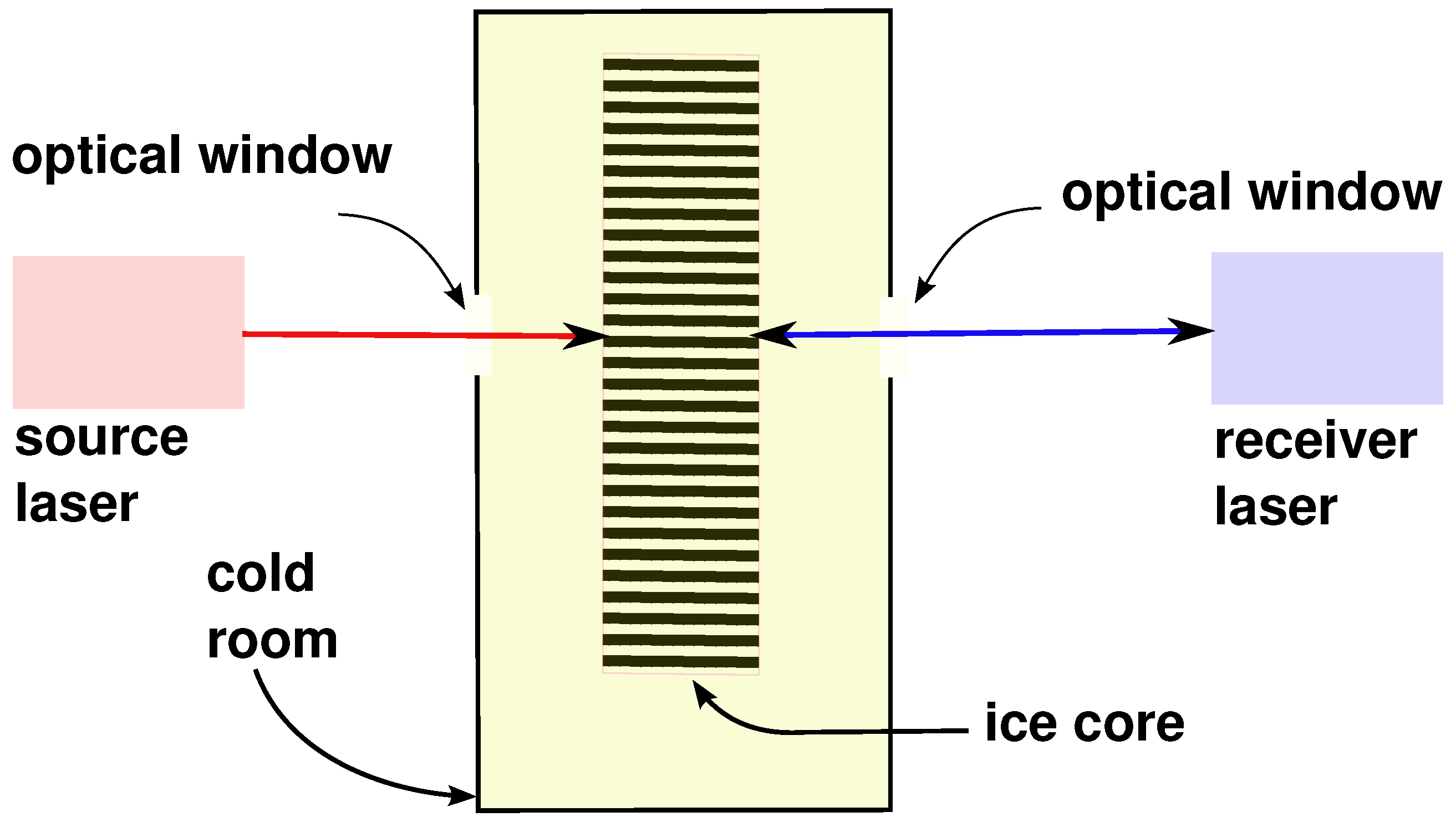
The laser used to excite the ultrasonic wavefield (i.e., the source laser) is a Nd:YAG (yttrium aluminum garnet) laser (1064 nm wavelength), model INDI from Spectra-Physics (Santa Clara, CA, USA) . Its pulse duration is 10 ns at 0.3 J per pulse, and the pulse repetition rate is 10 Hz. The source laser is positioned on one side of a cold room (Figure 1). The beam travels through a sapphire window into a cold room. The window has a viewing area of 32.4 cm and is 2.5 cm thick, made of three pieces of tempered glass. Sapphire is used because it mostly transmits the laser beam. This particular window is made by Norfab Inc (Plymouth, MN, USA) and is called Vu-Port. The cold room is from BioCold Environmental Inc. (Ellisville, MO, USA) and provides humidity and temperature control. The temperature is constantly kept at −20 ± 0.1 C for other snow science and ice experiments that occur separate to these laser ultrasound measurements.
Inside the cold room, we rest a core horizontally on a computer-controlled stage (Figure 1). This stage is manufactured by Newport Technologies (Irvine, CA, USA) and has been modified to perform at these cold temperatures, moving a standard 1 m long ice core at sub-mm resolution. The source laser beam is aimed at a point along the center of the core, the maximum diameter. The pulsed laser beam briefly (10 ns) heats the ice core surface without melting ice, causing local thermal expansion that is the source of an elastic wave [28]. Prior to hitting the ice surface, the beam is focused to a 1 mm beam diameter to excite elastic waves in the ultrasonic frequency range (e.g., [29]). At present, the core diameter can be any size, but the length cannot exceed 1 m.
On the opposite side of the ice core to the source laser beam, we point the receiver laser beam. We call this a zero-offset transmission-type experiment. We record transmissions of ultrasound from one side of the core to the other, through the center of the core. The receiver laser is a laser Doppler vibrometer (LDV) [30,31,32]. The LDV measures the Doppler shift induced in a monochromatic signal (i.e., the laser beam) reflected off of a moving target. In this case, the moving target is the ice surface on the opposite side of the core from the source laser. The surface motion is due to the arrival of the propagating elastic waves excited by the source laser. The particle velocity of the ice surface is measured by mixing the reflected receiver laser signal with a reference receiver laser signal internally in the LDV. The Doppler shift in the receiver laser signal is detected as a low frequency beat created by mixing the reflected and reference signals [33]. Thus, the target (i.e., surface-particle) velocity V is related to the Doppler shifted frequency according to
where c is the speed of light ( m/s) and and are the Doppler-shifted and transmitted frequencies, respectively. Note that this particle velocity V is different from the P-wave velocity we introduce later. Our Polytec PSV-500 Scanning LDV (Irvine, CA, USA) has a linear frequency response from the acoustic range into the high ultrasonic range at 2 MHz. After recording the particle velocity signal, numerical integration of the surface-particle velocity V results in surface-particle displacement, which we use to determine when the elastic wave arrives. All signal processing happens internally within the Polytec system, and we record only the surface-particle displacement as a function of time at single point in space. This laser is a HeNe Laser (633 nm wavelength). The operating temperature of both the source and receiver lasers is +5 C to +40 C, hence we cannot use the laser inside the cold room. Table 1 list the relevant parameters of this laser-based acquisition system.
The signal from the LDV is digitized at 16-bit precision on a Peripheral Component Interconnect (PCI) oscilloscope card from Alazar Tech (Pointe-Claire, Canada) at samples per second. The source laser, the receiver, and the stage are all controlled by an in-house LabView code. All systems are synced via Bayonet Neill–Concelman (BNC) cables and a trigger on the PCI card. The propagation time of the laser to/from the ice core surface is negligible compared to the time it takes the elastic waves to propagate through an ice sample.
To optimize the data quality, a small strip of reflective tape (∼0.5 cm wide) is applied to the ice-core surface on the receiver laser side. This reflective tape is composed of small glass beads that help reflect the 633 nm beam back to the LDV and improve the signal-to-noise ratio of the particle-displacement signal. The tape is applied by a warm hand, which acts to freeze the tape onto the core. It has been our experience that this application of tape can affect the ultrasonic waveforms in the ice. When the tape is poorly coupled, no signal is returned, as we will show in the next section. However, when the tape is properly coupled to the core it is invisible to the ultrasonic wavefield.
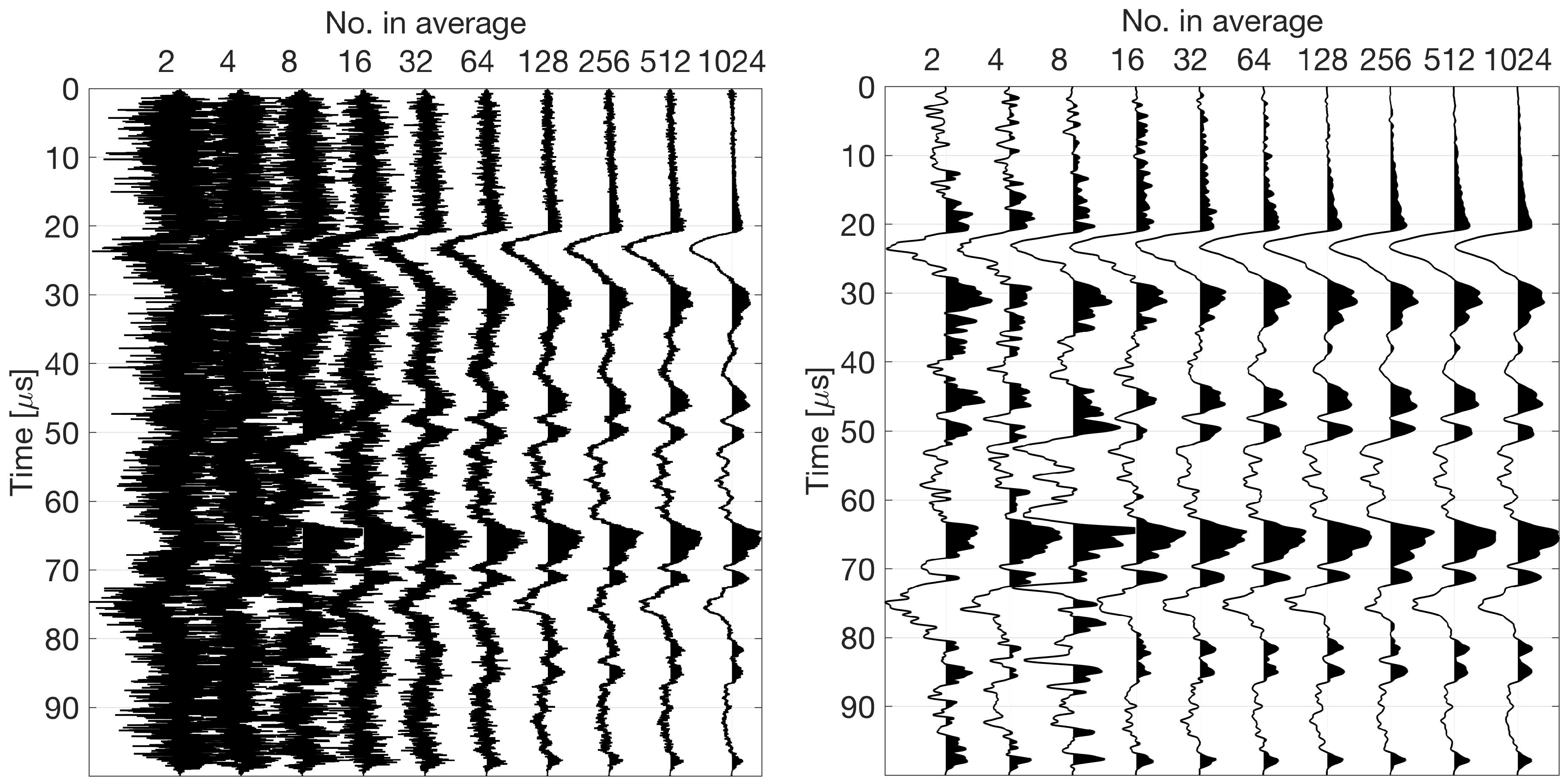
To further improve the signal-to-noise-ratio of the recorded waveforms, we average the waveforms from multiple recordings at the same position (Figure 2). This suppresses incoherent noise in individual recordings. We can do this because the lasers do not damage the sample, which would result in waveform changes with time. The waveforms in Figure 2 demonstrate that in the ultrasound frequency range of interest (1–1000 kHz), the random noise is well suppressed and the waveforms stabilize after about 32 traces are averaged. The data presented in the next section take 13 s per measurement to collect because we average 128 waveforms at a single point. This could be faster if we reduced the number of waveforms averaged, or if we used a PCI card that allows averaging in the buffer. With the current card we have to write each ultrasound trace from the card to the computer and then average. With the current acquisition system a 20 cm scan at 0.1 mm spatial sampling has 200 measurement points and takes 2600 s. It takes 3 s for the stage to move from one point to the next and come to rest. Therefore, moving the stage for 200 points take 600 s, and in total a 20 cm scan takes 3200 s (1 h). This time can be reduced with further improvements to hardware and an optimized sampling strategy.
From the surface displacement data, we can determine the arrival time of the various elastic wave types. For instance, we compute the P-wave velocity based on the core diameter and P-wave arrival time as , where is the P-wave arrival time. In the following data examples, the firn core is moved 0.5 mm between measurements, while the the ice core is moved 0.1 mm. We note that this is potentially over sampling and not optimized for making the fastest data collection. This is done however to highlight the data resolution and make high quality plots for this proof-of-concept study.
Finally, we note that the P-wavelengths in this experiment are ∼1–2 cm ( 3.4 km/s, 200 kHz), and for an 8 cm core we are in the far-field of ultrasonic wave propagation. Moreover, the source laser spot size is 1 mm, which at these wavelengths results in a plane-wave arrival on the opposite side of the core where the receiver laser measures surface displacements. Because of this we could neglect spherical wave propagation effects if we were to analyze the wave amplitudes, but we note that amplitude analysis is not part of this study of travel times and velocity.
3. Results
We have tested two ice cores (Figure 3) with different burial depths and strain histories using the laser ultrasound system. Both cores are ∼8 cm in diameter, and neither core has obvious visible layers. Both cores were provided by the Climate Change Institute at the University of Maine (Orono, ME, USA).
3.1. ITASE-01-3B Firn Core
The ITASE-01-3B core is a firn core collected during the International Trans Antarctic Scientific Expedition (e.g., [34]). The core was collected at 78.12 S, 95.65 W from an elevation of 1620 m. Our sample is a small section of the B core from depth 68–70 m. This core is not continuous and therefore we scanned one of the larger continuous sections of the core (depth 69.65 to 69.82 m) over which there is a presumed annual layer boundary. We collected an ultrasound measurement every 0.5 mm.
The ITASE-01-3 core was extensively studied by Dixon et al. [14]. The core was dated by counting seasonal signals and verified by volcanic signals from large historical tropical events. The section of core we scanned covers the 1860–1861 AD boundary at 69.69 m depth. This age was taken from published chemistry data [35]. The bulk density is 0.789–0.801 g/cm, and analysis by 400 MHz radar indicates horizontal layering in this area of the core, orthogonal to the core axis. A photograph of this section of core is shown in Figure 4. There are no visible annual layers.
The complete ultrasound scan is shown in Figure 5, while a zoom around the first arriving P wave is shown in Figure 6. Multiple wave types are visible in the ultrasonic wavefield (e.g., S, P, PP (a reflected P wave), Rayleigh, and scattered waves from internal heterogeneities and the edge of the core in Figure 5). The characteristic poor wavefield recording due to poor tape coupling also visible. The P-wave arrival time is roughly 25 s (Figure 6), and the core diameter was measured to be 8.2-cm. From this we compute a P-wave velocity of ∼3.2 km/s. We note that the core diameter did not vary significantly (<3 mm) over the section scanned. A variation of a few mm in the diameter would result in velocity variations of a few percent. We observe velocity variations near 10%, and therefore we are confident these variations are due to real structure in the ice itself rather than changes in the core diameter.
To automate the process of picking the P-wave arrival time on each waveform, we use a window-based energy-ratio picking algorithm. Examples of commonly used window-based energy-ratio algorithms include the short- and long-time average ratio (STA/LTA) [36,37,38] and the modified energy ratio (MER) [39,40,41]. The STA window is sensitive to rapid fluctuations in the amplitude of the time series, while the LTA window provides information about the background noise. The maximum in the derivative of this STA/LTA function is assumed to be related to the arrival of an ultrasonic wave. Instead of the traditional STA/LTA method, we use the MER method to automatically pick the time of the direct P-wave arrival. MER is an extension of STA/LTA in which the pre- and post-sample windows are of equal size [42]. This method has been shown to out-perform the STA/LTA detection algorithm, especially when the signal-to-noise ratio is low [39]. The solid red line in Figure 6 indicates the automatically picked first arrivals using the MER picker. The window length we use in the MER picker is 0.5 s and the exponential coefficient is three.
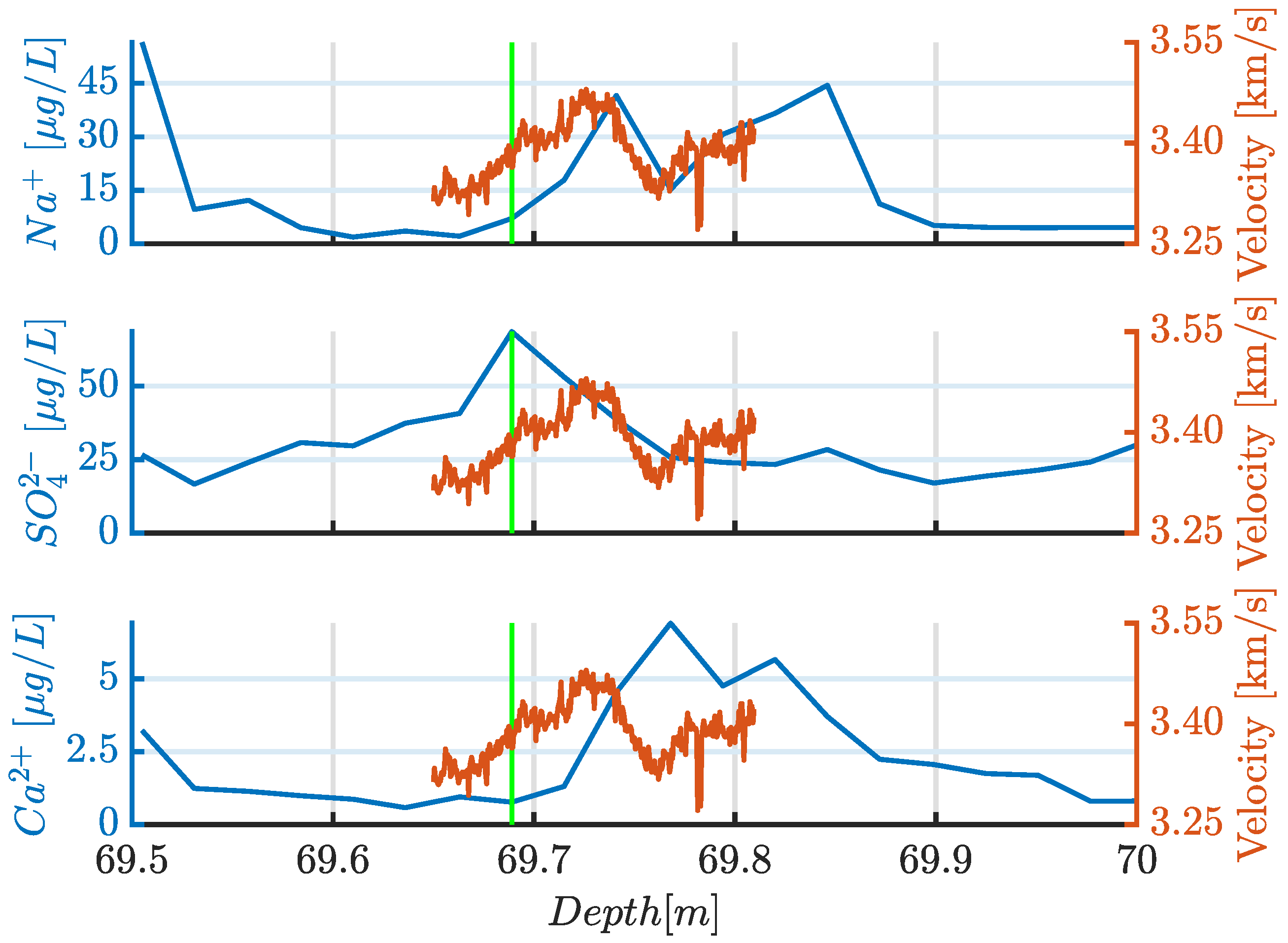
From the arrival time pick at each measurement point, we compute the velocity as a function of depth (assuming a constant diameter of 8.2 cm). We overlay these velocity data onto a plot of chemistry data previously collected along this core (Figure 7). The green vertical line indicates the estimated layer boundary at 1860–1861 AD, and while there is no established physical relationship between P-wave velocity and any of the chemistry data, we observe ice velocity variations on the same length scale as the chemistry data, specifically the Na concentration. Keeping in mind that this core comes from the southern hemisphere, the green line indicates the months of December and January, which is Summer. Moving from summer to fall, we see a steady increase in the P-wave velocity and then a sharp decrease and another increase. We suspect that this increase is related to a crystal structure that is then repeated over the next annual cycle. We note that previous studies have observed strong correlations between Ca concentration and density (e.g., [43,44]), but it is impossible to make concrete conclusions based on this small section of firn core. Future studies should investigate the density, elastic moduli, and chemical impurity concentrations to determine if any (strong) correlations exist and are related to seasonal phenomena in the snowpack. We consider this topic more in the Section 4.
3.2. 2MBIA09-13
Ice core 2MBIA09-13 is from a surface transect through the main icefield at Allan Hills, Antarctica (76.71 S, 159.29 E). This particular section of core consists of bubbly ice collected from the ablation zone of a blue-ice area. This section of core is estimated to be ∼107,000 years old [45], and the time-scale and water isotope data are published online [46]. The bulk density is 0.899–0.901 g/cm, and field observation of an exposed tephra layer indicate a dip in core layers of ∼17 degrees from horizontal [45]. This core has previously been buried and is now exhumed in its current location. This means the stress-strain history of this core is likely not just due to overburden as in ITASE-01-3B. A photo of part of the core is shown in Figure 4. Spaulding et al. [45] report a variety of time resolutions within the ice in this area (i.e., ∼171–858 years/m), which corresponds to average annual layer thicknesses in the range of 0.6 to 2.9 cm. Neither the seasonal structure, nor the dipping layer structure within this core is visible.
We recorded ultrasound waveforms every 0.1 mm from depth 10.4 m to 10.48 m in core 2MBIA09-13 (Figure 8). Again we average 128 waveforms at each position along the core. The amplitude variations at each depth are possibly due to bubbles, dust, other chemical impurities, or some combination thereof. We cannot say for sure at this time, but they do not resemble tape coupling problems as in Figure 5. Note the oscillating behavior of the amplitudes and the apparent changes in frequency content of the waveforms, especially the surface waves arriving after 40 s. The arrival just after 20 s is the direct P wave (arriving earlier than in the firn core) followed by PP reflections and shear waves. Many point diffractions also exist, indicating that scattering due to impurities (chemical or bubbles) is occurring.
The velocity variation in the P-wave arrival is less dramatic in this core than in the ITASE core. This is likely due to the different stress-strain histories and maximum depth of burial, which have influenced the density and elastic moduli of ice differently compared to firn. However, we can still measure arrival time differences along the core by considering the average differences of all waves— the fast P and slower S and Rayleigh waves. Rather than picking the arrival time of the direct P wave, we use cross correlation of the entire waveforms to estimate an average time lag between the most shallow measurement point and all others. Prior to cross correlation we bandpass filter the data between 1 and 250 kHz and normalize each trace based on its maximum amplitude. We then apply a moving average smoothing to each trace, averaging each trace with both traces on either side (Figure 9). This processing helps balance the amplitudes across the entire scan at the cost of some small depth and time smearing, but obvious variations in arrival time still exist in the processed data (Figure 9).
It is not possible to convert relative time lag measurements made in this way into velocity because we average over multiples types of waves. However, we can still analyze these time lags in order to look for coherent structures within the core. The time lags associated with the maximum correlation coefficient are shown in the top of Figure 10. The time lag is relative to the trace at the top of the core (depth 10.4 m). There are five outliers, indicated by the large spikes. We eliminate these with the Thompson out-lier test [47]. The time lags after out-lier removal and linear trend removal are shown in the bottom plot of Figure 10. The red line in the top plot indicates the measured linear trend in the data. This line has a slope of −2.881 s/m, indicating an average velocity increase with depth for all wave types. Gow et al. [48] found a similar increase in P-wave velocity with depth and attributed this to hydrostatic compression of entrapped bubbles.
After removing the linear trend, we fit a sine function using least-squares and found a best-fit wavelength of ∼2 cm. This function is overlain on the processed time lag data in the bottom of Figure 10. Based on the range of layer thicknesses provided by Spaulding et al. [45], if we assume seasonal layers alternate between slow and fast velocities, then this sine function appears to explain the data. Under this assumption, we interpret the weak fluctuations in time lags, occurring approximately every ∼1 cm, as seasonal layers. Because the layers are not identical in thickness, it is difficult to fit a curve exactly to the data (e.g., amplitude and phase). Furthermore, these layers dip on the order of 17 degrees [45], which also makes the interpretation difficult if we only use one scan along a single side of the core. Therefore, we performed a rotational scan around the core at a single depth to look at the velocity variations caused by the dipping layers.
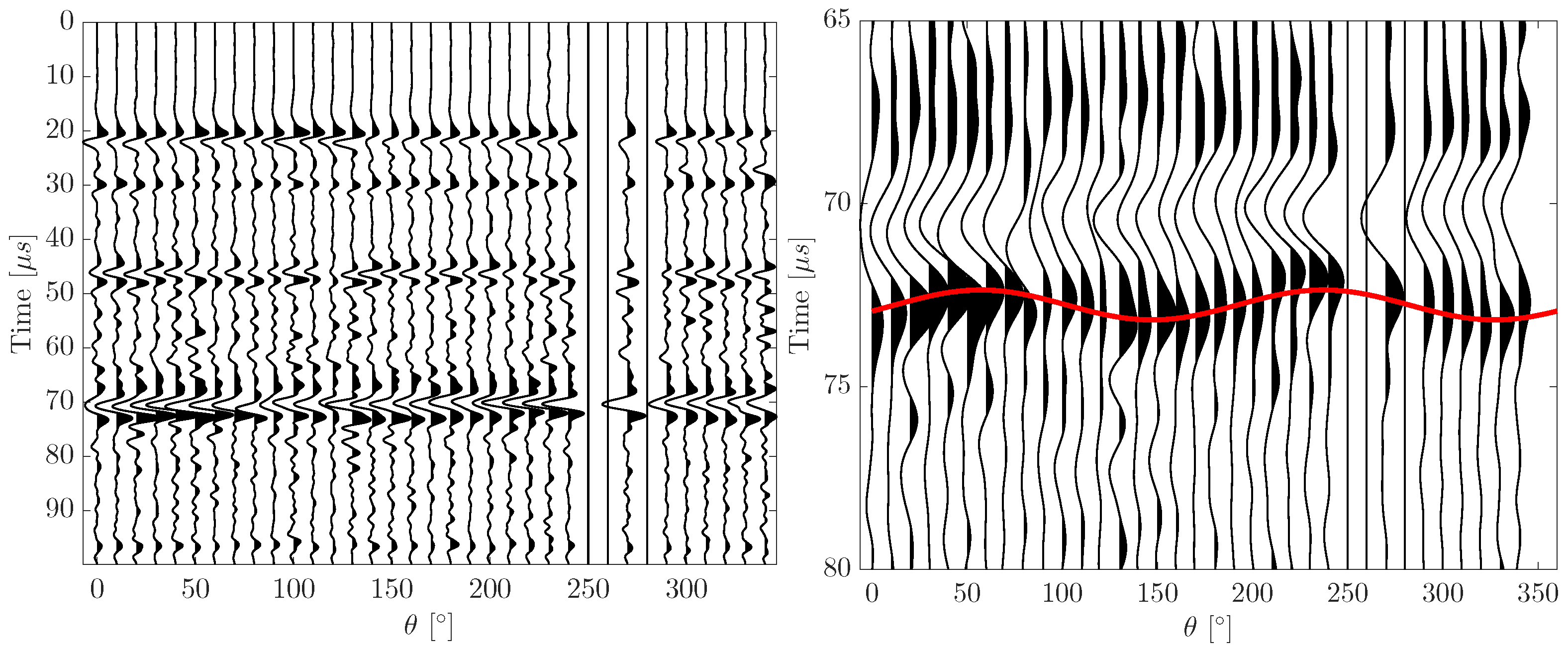
We made ultrasonic measurements every 10 deg around the circumference of the 2MBIA09-13 core (Figure 11). For reference, the data in Figure 8 and Figure 9 were recorded along the 30 deg angle. Three noisy waveforms are muted (i.e., set to zero amplitude for all time). These bad data occur due to poor tape coupling or the presence of a bubble right at the surface of the core. The P-wave travel time differences are small in this section of core. Therefore, we instead analyze the Rayleigh surface wave that travels a longer path around the core surface and at a slower velocity because this wave experiences larger time differences in the presence of velocity variations.
A zoom around the Rayleigh wave is shown in Figure 11. For materials with anisotropy, we expect the velocity to vary as , meaning that there are two fast directions (actually opposite directions) and two slow directions around the core. We picked the maximum amplitude of the Rayleigh wave at each angle and then fit the function to the data using least-squares. The red curve in Figure 11 shows the curve predicted by the best fit model. We see two slow directions at 180 and 360 degrees and two fast directions around 90 and 270 degrees.
4. Discussion
There is a wealth of knowledge in the seismology community regarding layered media and tilted layered media. A model with horizontal homogeneous layers is known as a vertical transversely isotropic (VTI) medium and a model with tilted homogeneous layers is known as tilted transversely isotropic (TTI) (e.g., [49]). These models have a vertical symmetry axis or a tilted symmetry axis, respectively, and observations of wave velocity from multiple azimuths and dips can be used to estimate the symmetry axis orientation. Another stratigraphic complication typically found in deep ice is folding. Ice deformation near the bed of ice sheets and glaciers can be very complicated, leading eventually to overturning of the stratigraphic column (e.g., [50] and references therein). In this case, the proposed ultrasonic method will suffer the same fate as other stratigraphic estimation methods. It will likely be difficult to determine where ice has become overturned from the single point measurements of cores. However, in the future we can combine rotational and along axis scans to characterize the entire 3D structure of stratigraphic layers in the core, but for now the analysis stops at the observation of anisotropy in the core, which we suspect is due to the dipping layers.
After the experiments were performed on these two cores, careful visual inspection revealed no damage was caused by the acquisition process, in either geometry (i.e., rotational or axial scans). Moreover, the waveforms repeatedly recorded at a single position in space did not change through time as more wavefield measurements were made (Figure 2). Therefore, this laser-based method can be used to observe ultrasonic wave propagation in standard 1 m ice-core sections in a non-destructive and non-invasive fashion at (sub)millimeter resolution. This type of approach allows further chemical and other analyses to be performed without contamination. There are also numerous advantages to this non-contacting ultrasound acquisition system over conventional systems that use contacting piezo-electric transducers. Attaching transducers to the ice core is time consuming and prone to coupling variations. One can also damage the ice core during transducer removal. As we have demonstrated here (Figure 6), we can still have coupling problems because we use reflective tape, but this laser-base method enables much higher spatial sampling of the ultrasonic wavefield compared to traditional transducers and requires less acquisition time.
Another important factor of this non-contacting system to consider is that as the ultrasound wavelength decreases (or frequency increases) relative to the size of heterogeneity, scattering from the micro-structure becomes important and the transducers themselves begin to act as scatterers, disturbing the measured wave fields. Moreover, the transducers can introduce mechanical ringing into the measured wavefields and lead to mis-interpretations of arrivals. The laser-based system eliminates these problems completely, and while we have only analyzed the direct P (ITASE core) and Rayleigh waves (MBIA09) in this study, analysis of scattered waves will also provide interesting information about the elastic structure of the ice cores in the future. Lastly, we wish to discuss in detail why we think future observations of ice core ultrasound velocity variations will be useful for ice core stratigraphy and mechanics analysis.
4.1. Elastic Moduli and Ultrasonic Velocities
Up to now elastic moduli have not been used to infer seasonal layering in ice and firn cores. However, we think these physical parameters are worthy of further investigation. While we can not directly sample the elastic moduli with the laser ultrasound system, we can measure the velocity of various elastic wave types that propagate in solid materials at ultrasonic frequencies. For an isotropic medium, two elastic constants and the density define the elastic wave propagation velocities. The compression- or P-wave has a longitudinal particle motion, and the velocity () is related to the elastic moduli as , where is the density, K is the bulk modulus and is the shear modulus. The shear- or S-wave has a transverse particle motion, and the velocity () is related to the elastic moduli as . P- and S-waves are both body waves, meaning they travel through the solid material.
Surface waves also exist in solids with boundaries. A Rayleigh wave is a surface wave composed of a combination of longitudinal and transverse particle motions [51]. Because surface-wave geometric spreading happens over a surface—rather than over a volume as for body waves—Rayleigh waves are often high-amplitude features in the observed wavefield. By solving the boundary conditions for an elastic wave trapped at a surface, the Rayleigh wave velocity, , can be related to and such that the following condition is satisfied [51]:
with the requirement that . This relation eliminates the need to measure , and independently. If two wave velocities are measured, the real roots of Equation (2) yield the velocity of the third wave type [52]. If the density of the ice is known, then measurements of P- and S- or Rayleigh-wave velocities can be used to infer the shear and bulk moduli.
An isotropic medium can also be represented by Young’s modulus E and Poisson’s ratio (e.g., [52]). Young’s modulus relates the magnitude of strain in the direction of an applied stress, while Poisson’s ratio relates the strain in directions orthogonal to the stress (e.g., [51]). We can estimate E and from the propagation velocities of P and S waves and the density:
In this article, we present observations of variations in P-wave velocity across a firn core as measured by this novel non-contacting laser ultrasound system. We also present observations of P, PP, S, and Rayleigh waves in both firn and ice cores, but we leave elastic moduli estimation and correlation to physical ice properties (e.g., bubble or impurity concentration) for future study. However, we can speculate as to why we think that elastic moduli will be useful estimators of seasonal layering in ice and firn cores.
4.2. Elastic Moduli and Density Variations
Benson [53] found that stratification of snow results from variations in the conditions of deposition and subsequent metamorphism. For example, Freitag et al. [44] observed thin high-density layers in an Antarctic firn core related to wind crusts. Summer layers can also show evidence of surface melt and can be coarser-grained with generally lower density and hardness values than winter layers [53]. Alley et al. [54] and Alley et al. [17] confirmed that summertime solar heating of near surface snow in central Greenland causes mass loss and grain growth, while the underlying snow remains undisturbed and retains its fine grain structure. Moreover, the onset of the fall season is usually identified by an abrupt increase in density and hardness accompanied by a decrease in grain size [53]. This stratigraphic discontinuity in density should have an impact on elastic velocities and has previously been used as the annual reference plane [53], a key parameter when creating ice core depth-age relationships.
Gerland et ak. [55] combined ECM and water isotope data in a detailed study of density at Berkner Island, Antarctica, and found that the density of firn, even over seasons, can be quite heterogeneous above the firn-ice transition. However, prior to discussing the density variations with depth observed by Gerland et al. [55], it is worth summarizing the process of how snow turns into ice in the upper layer of ice sheets as described by Cuffey and Paterson [56]. When there is no surface melt this process can be divided into four sections. In the first section, settling is the dominant densification process until a density of 0.55 g/cm. In the second section, recrystallization and deformation control densification until a density of 0.73 g/cm. In the third section, densification is dominated by creep until a density of 0.83 g/cm. At this point the air spaces between grains close and bubbles form. This defines the firn-ice transition and beginning of the fourth section. Below this, the ice can reach a maximum density of ∼0.91 gm/cm.
In what Gerland et al. [55] defined as sections one and two in the Berkner core, they observed densification rates of 0.017 gm/cm/m and 0.006–0.0080 gm/cm/m respectively. The rate then decreased through sections three and four before ceasing around 100 m depth. In sections one and three, Gerland et al. [55] observed large seasonal variations in the ice density, up to 0.05 gm/cm. However, the more interesting observation was a change in the sense of density between winter and summer layers. While numerous studies have observed lower density summer firn layers compared to winter layers in Greenland (e.g., [57]) and Antarctica, Gerland et al. [55] found that at a depth of ∼30 m, the summer layers became more dense than winter layers. This could lead to misinterpretation of ultrasonic data, but it is worth noting, however, that the winter and summer layers still alternated between low and high density on a seasonal basis. It is also still unknown how the elastic moduli should vary with depth.
As is apparent in the equations for P- and S-wave velocity, density is a key parameter when considering elastic wave velocities in an ice core. Density can be measured by gamma-absorption [55,58] or by X-ray computer tomography (X-CT [44]). As others have also reported (e.g., [43]), Freitag et al. [44] observed a correlation between density and calcium ion concentration. They went on to suggest that the relationship between this particular impurity and density is a universal feature of polar firn and that the calcium ion concentration can serve as a proxy to describe quantitatively the effect of the impurities on densification. In sections of core that have not undergone strain, such that no crystal fabrics have developed, we expect that variations in elastic wave speeds should be sensitive to variations in density, shear strength, and perhaps even impurities.
In regard to shear strength in firn, summertime solar heating can warm the snow surface on ice sheets and glaciers. Due to the colder snow and firn beneath, a vertical temperature gradient is created in the near surface snow [17,54]. In the fall season, early snowfall insulates the warmer summer surface, and combined with the cold fall air temperatures, causes another large vertical temperature gradient in the opposite direction (e.g., [59]). Both of these vertical temperature gradients cause vapor pressure gradients, which drive temperature gradient metamorphism in the near surface snow, resulting in faceted snow grains (e.g., [60]). The underlying snow however remains undisturbed and retains its fine grain texture.
In a NorthGRIP case study conducted on a 1.2 m long core from 301 m depth, Svensson et al. [43] observed that each year there was strong seasonal variability in crystal areas (>30%) and that ice deposited during spring had smaller than average (6.7 mm) crystals. The crystal areas were also compared to chemical impurity concentrations and found to correlate the best with Ca. At this depth, Svensson et al. [43] did not observe any variation in the c-axis orientation of crystals, known to cause elastic-wave velocity anisotropy when aligned in a fabric (e.g., [61]). We speculate that these grain-size differences might also cause variations in the structural and mechanical properties (e.g., elastic moduli). Moreover, these faceted layers can be weak in shear (e.g., [60]), but because of the preferred vertical grain growth due to the vertical vapor pressure gradients, this facet layer is strong in compression, and therefore persist during burial. Finally, Gammon et al. [62] find that the variation in the elastic properties of isotropic polycrystalline ice in the temperature range between −50 C and near the melting point should lie below 10%, indicating only a small temperature dependence. Gammon et al. [62] also suggest that the elastic properties may vary considerably with the impurity content of ice. Therefore, the ultrasonic wavefield may be sensitive not only to density and elastic moduli, but also impurity concentration and to a small degree temperature. Within each seasonal cycle, we expect to observe slow and fast regions in terms of ultrasonic velocities related to the variations in crystal size, orientation, bubble size and density, and impurity concentrations. It is possible that this method will be sensitive to a number of ice properties and requires further detailed investigation to fully understand how the ultrasonic wavefield interacts with these different properties.
4.3. Velocity Anisotropy and Preferred Crystal Orientation Fabrics
As snow is compacted and layers thin due to ice flow (e.g., [13]), annual stratigraphy becomes difficult to identify and ice crystal fabrics develop. Ice crystal fabrics have been characterized at the large scale using seismic, sonic, and ultrasonic experiments (e.g., [61,63,64,65,66,67,68]). This fabric is due to the alignment of the ice crystal c-axes over time and leads to structural anisotropy in the elastic moduli and wave velocities. Early on Kohnen and Gow [69] observed ultrasonic velocity variations up to 140 m/s in deep ice from Byrd Station and correlated this velocity anisotropy to c-axis alignment in the crystal fabric. Later Gow et al. [48] identified similar velocity anisotropy due to the c-axis fabric. They used ultrasound to measure velocity along both parallel and orthogonal directions to the core axis every 10 m from the surface down to ∼3000 m depth in the GISP2 core.
An interesting feature of deep ice is cloudy bands. Gow and Williamson [65] reported the existence and basic properties of cloudy bands and observed that the fine-grained structure and high anisotropy of such bands enable localized zones of intense shearing, which may contribute significantly to the flow of the ice sheet. Such extensive shearing along discrete strata situated well above bedrock could cause differential layer thinning and seriously distort the stratigraphy, making the dating and interpretation of climate records extremely complicate [50]. Of note is that in glacial ice, Bendel et al. [70] determined that these cloudy bands have high bubble density and small bubble size and are linked to layers with high impurity content. Bendel et al. [70] also attribute impurities as a controlling factor on the formation and distribution of bubbles in glacial ice. It is currently unknown if the ultrasonic wavefield is sensitive to such properties as bubble size and density. According to Faria et al. [50], cloudy bands continue to challenge our understanding of ice mechanics and microstructure, even with novel methods of observation and modeling casting new light on this issue [18,19,71,72,73]. It is, therefore, timely that this laser-based ultrasound method is developed as another tool to aid the mechanical study of ice core structure.
While seismic, sonic, and ultrasonic experiments have proven successful for determining preferred ice fabrics due to strain history, they did not use ultrasound as a high-resolution tool to identify seasonal or annual layer structure. We mention these studies of orientation fabric only for completeness, and we stop the discussion of crystal fabrics and velocity here. However, we note that the novel laser-ultrasound method presented here probes the core with mm-scale resolution rather than m-scale resolution, thus sensing variations in the elastic velocity of the ice at finer spatial scales than previous ultrasound studies.
4.4. Anelasticity
Vaughan et al. [74] used resonant ultrasound spectroscopy to make quantitative estimates of elastic and anelastic properties of ice. These properties aid calibration of active and passive seismic data gathered in the field. They found that the elastic constants and attenuation constant in man-made polycrystalline isotropic ice cores decreased (reversibly) with increasing temperature. They also determined that P-wave velocity and attenuation proved the most sensitive to temperature, indicating pre-melting of the ice. In the work presented here, we held the temperature constant, but note that we could in theory vary the temperature in the cold room to make similar measurements with the laser system.
5. Conclusions
Laser-based ultrasound provides a non-destructive tool that may compliment studies of the physical properties of ice cores. We utilize a non-contacting laser-ultrasound measurement system integrated with a climate-controlled cold room and computer-controlled mechanical stage. We demonstrate that this laser-based ultrasound acquisition system works with both ice and firn cores. Initial measurements indicate contrasts in elastic properties within two Antarctic cores. The velocity variations we observe in both cores cannot be due to small variations in the core diameter. Thus these observations are taken to indicate actual elastic property variations in the cores on the scale of millimeters.
Extraction of seasonal signals from ice core 2MBIA09-13, which has dipping layers, is complicated because the stress-strain history is not just increasing overburden pressure. While we cannot directly relate observed velocity variations to known seasonal markers, we do observe variations in wave velocity on the same length scales as other physical properties (e.g., chemistry [45]). We also observe an increasing velocity with depth, perhaps related to the overburden stress history and densification during burial of the core. Chemical evidence of the transition of an annual layer in firn core ITASE-01-3B, with flat horizontal stratigraphy, also correlates with ultrasound velocity variations in term of spatial wavelength. Finally, we observe velocity anisotropy in the Rayleigh wave due to known dipping layers in the 2MBIA09-13 core and demonstrate that linear ultrasound scans can be aided by rotational scans around the axis of the core to determine fast and slow directions when the sample is anisotropic.
We propose that this system can eventually be used to create high-resolution maps of ultrasound velocities and (an)elastic moduli (if the density is known) through imaging methods like tomography. Furthermore, these measurements are achieved without disturbing the integrity of the sample, such that complementary dating methods and stratigraphic analysis can be performed on the same core. In the future, rotational scans at multiple depths will, in principle, allow us to image the full 3D elastic structure of ice cores at very high resolution. With density estimates from other techniques, we should be able to directly estimate the isotropic elastic moduli using ultrasonic waveforms recorded with this new laser-based method.
Acknowledgments
This research is supported by NSF-EAR MRI Award 1229722, and we thank Nicky Spaulding and Paul Mayewski for their support. T.D. Mikesell acknowledges support for this research from Boise State University. The authors thank four anonymous reviewers for comments that helped improve the quality of this article.
Author Contributions
T.D.M., K.v.W., A.K. and H.-P.M. conceived and designed the experiment. T.D.M., L.T.O. and K.v.W. carried out the data collection and reduction. All authors contributed to the data analysis and manuscript preparation.
Conflicts of Interest
The authors declare no conflict of interest. The founding sponsors had no role in the design of the study; in the collection, analyses, or interpretation of data; in the writing of the manuscript, and in the decision to publish the results.
Abbreviations
The following abbreviations are used in this manuscript:
| LLS | Laser-Light Scattering |
| ECM | Electrical Conductivity Measurement |
| LDV | Laser Doppler Vibrometer |
| PCI | Peripheral Component Interconnect |
| BNC | Bayonet Neill–Concelman |
| STA | Short-Time Average |
| LTA | Long-Time Average |
| MER | Modified Energy Ratio |
References
- EPICA Community Members. Eight glacial cycles from an Antarctic ice core. Nature 2004, 429, 623–628. [Google Scholar]
- McConnell, J.R.; Lamorey, G.W.; Lambert, S.W.; Taylor, K.C. Continuous Ice-Core Chemical Analyses Using Inductively Coupled Plasma Mass Spectrometry. Environ. Sci. Technol. 2002, 36, 7–11. [Google Scholar] [CrossRef] [PubMed]
- Winstrup, M.; Svensson, A.M.; Rasmussen, S.O.; Winther, O.; Steig, E.J.; Axelrod, A.E. An automated approach for annual layer counting in ice cores. Clim. Past 2012, 8, 1881–1895. [Google Scholar] [CrossRef]
- Rasmussen, S.O.; Andersen, K.K.; Svensson, A.M.; Steffensen, J.P.; Vinther, B.M.; Clausen, H.B.; Siggaard-Andersen, M.L.; Johnsen, S.J.; Larsen, L.B.; Dahl-Jensen, D.; et al. A new Greenland ice core chronology for the last glacial termination. J. Geophys. Res. Atmos. 2006, 111, 1–16. [Google Scholar] [CrossRef]
- Sigl, M.; McConnell, J.R.; Layman, L.; Maselli, O.; McGwire, K.; Pasteris, D.; Dahl-Jensen, D.; Steffensen, J.P.; Vinther, B.; Edwards, R.; et al. A new bipolar ice core record of volcanism from WAIS Divide and NEEM and implications for climate forcing of the last 2000 years. J. Geophys. Res. Atmos. 2013, 118, 1151–1169. [Google Scholar] [CrossRef]
- Hammer, C.U. Acidity of polar ice cores in relation to absolute dating, past volcanism, and radio echoes. J. Glaciol. 1980, 25, 359–372. [Google Scholar] [CrossRef]
- Hammer, C.U. Initial direct current in the buildup of space charges and the acidity of ice cores. J. Phys. Chem. 1983, 87, 4099–4103. [Google Scholar] [CrossRef]
- Taylor, K.C.; Hammer, C.U.; Alley, R.B.; Clausen, H.B.; Dahl-Jensen, D.; Gow, A.J.; Gundestrup, N.S.; Kipfstuhl, J.; Moore, J.C.; Waddington, E.D. Electrical conductivity measurements from the GISP2 and GRIP Greenland ice cores. Nature 1993, 366, 549–552. [Google Scholar] [CrossRef]
- Moore, J.; Paren, J.; Oerter, H. Sea salt dependent electrical conduction in polar ice. J. Geophys. Res. 1992, 97, 19803–19812. [Google Scholar] [CrossRef]
- Wilhelms, F.; Kipfstuhl, J.; Miller, H.; Heinloth, K.; Firestone, J. Precise dielectric profiling of ice cores: A new device with improved guarding and its theory. J. Glaciol. 1998, 44, 171–174. [Google Scholar] [CrossRef]
- Wilhelms, F. Explaining the dielectric properties of firn as a density-and-conductivity mixed permittivity (DECOMP). Geophys. Res. Lett. 2005, 32, 1–4. [Google Scholar] [CrossRef]
- Weißbach, S.; Wegner, A.; Opel, T.; Oerter, H.; Vinther, B.M.; Kipfstuhl, S. Spatial and temporal oxygen isotope variability in northern Greenland—Implications for a new climate record over the past millennium. Clim. Past 2016, 12, 171–188. [Google Scholar] [CrossRef]
- Andersen, K.K.; Svensson, A.; Johnsen, S.J.; Rasmussen, S.O.; Bigler, M.; Röthlisberger, R.; Ruth, U.; Siggaard-Andersen, M.L.; Peder Steffensen, J.; Dahl-Jensen, D.; et al. The Greenland Ice Core Chronology 2005, 15–42 ka. Part 1: Constructing the time scale. Quat. Sci. Rev. 2006, 25, 3246–3257. [Google Scholar] [CrossRef]
- Dixon, D.; Mayewski, P.A.; Kaspari, S.; Sneed, S.; Handley, M. A 200 year sub-annual record of sulfate in West Antarctica, from 16 ice cores. Ann. Glaciol. 2004, 39, 545–556. [Google Scholar] [CrossRef]
- Della Lunga, D.; Muller, W.; Rasmussen, S.O.; Svensson, A. Location of cation impurities in NGRIP deep ice revealed by cryo-cell UV-laser-ablation ICPMS. J. Glaciol. 2014, 60, 970–988. [Google Scholar] [CrossRef]
- Sneed, S.B.; Mayewski, P.A.; Sayre, W.G.; Handley, M.J.; Kurbatov, A.V.; Taylor, K.C.; Bohleber, P.; Wagenbach, D.; Erhardt, T.; Spaulding, N.E. Instruments and Methods New LA-ICP-MS cryocell and calibration technique for sub-millimeter analysis of ice cores. J. Glaciol. 2015, 61, 233–242. [Google Scholar] [CrossRef]
- Alley, R.B.; Shuman, C.A.; Meese, D.A.; Gow, A.J.; Taylor, K.C.; Cuffey, K.M.; Fitzpatrick, J.J.; Grootes, P.M.; Zielinski, G.A.; Ram, M.; et al. Visual-stratigraphic dating of the GISP2 ice core: Basis, reproducibility, and application. J. Geophys. Res. Oceans 1997, 102, 26367–26381. [Google Scholar] [CrossRef]
- Svensson, A.; Nielsen, S.W.; Kipfstuhl, S.; Johnsen, S.J.; Steffensen, J.P.; Bigler, M.; Ruth, U.; Röthlisberger, R. Visual stratigraphy of the North Greenland Ice Core Project (NorthGRIP) ice core during the last glacial period. J. Geophys. Res. D Atmos. 2005, 110, 1–11. [Google Scholar] [CrossRef]
- Takata, M.; Iizuka, Y.; Hondoh, T.; Fujita, S.; Fujii, Y.; Shoji, H. Stratigraphic analysis of Dome Fuji Antarctic ice core using an optical scanner. Ann. Glaciol. 2004, 39, 467–472. [Google Scholar] [CrossRef]
- Ram, M.; Illing, M. Polar ice stratigraphy frotn laser-light scattering: Scattering frotn meltwater. J. Glaciol. 1994, 40, 504–508. [Google Scholar] [CrossRef]
- Bramall, N.E.; Bay, R.C.; Woschnagg, K.; Rohde, R.A.; Price, P.B. A deep high-resolution optical log of dust, ash, and stratigraphy in South Pole glacial ice. Geophys. Res. Lett. 2005, 32, L21815. [Google Scholar] [CrossRef]
- Ackermann, M.; Ahrens, J.; Bai, X.; Bartelt, M.; Barwick, S.W.; Bay, R.C.; Becka, T.; Becker, J.K.; Becker, K.H.; Berghaus, P.; et al. Optical properties of deep glacial ice at the South Pole. J. Geophys. Res. Atmos. 2006, 111, 1–26. [Google Scholar] [CrossRef]
- Meese, D.A.; Gow, A.J.; Alley, R.B.; Zielinski, G.A.; Grootes, P.M.; Ram, M.; Taylor, K.C.; Mayewski, P.A.; Bolzan, J.F. The Greenland Ice Sheet Project 2 depth-age scale. J. Geophys. Res. Oceans 1997, 102, 411–423. [Google Scholar] [CrossRef]
- Donarummo, J. Possible deposit of soil dust from the 1930’s U.S. dust bowl identified in Greenland ice. Geophys. Res. Lett. 2003, 30, 18–21. [Google Scholar] [CrossRef]
- McGwire, K.C.; Hargreaves, G.M.; Alley, R.B.; Popp, T.J.; Reusch, D.B.; Spencer, M.K.; Taylor, K.C. An integrated system for optical imaging of ice cores. Cold Reg. Sci. Technol. 2008, 53, 216–228. [Google Scholar] [CrossRef]
- Taylor, K.C.; Alley, R.B.; Meese, D.A.; Spencer, M.K.; Brook, E.J.; Dunbar, N.W.; Finkel, R.C.; Gow, A.J.; Kurbatov, A.V.; Lamorey, G.W.; et al. Dating the Siple Dome (Antarctica) ice core by manual and computer interpretation of annual layering. J. Glaciol. 2004, 50, 453–461. [Google Scholar] [CrossRef]
- Svensson, A.; Andersen, K.K.; Bigler, M.; Clausen, H.B.; Dahl-Jensen, D.; Davies, S.M.; Johnsen, S.J.; Muscheler, R.; Parrenin, F.; Rasmussen, S.O.; et al. A 60,000 year Greenland stratigraphic ice core chronology. Clim. Past 2008, 4, 47–57. [Google Scholar] [CrossRef]
- Scruby, C.; Drain, L. Laser Ultrasonics Techniques and Applications; CRC Press: Boca Raton, FL, USA, 1990; p. 462. [Google Scholar]
- Scales, J.; Malcolm, A. Laser characterization of ultrasonic wave propagation in random media. Phys. Rev. E 2003, 67, 1–7. [Google Scholar] [CrossRef] [PubMed]
- Nishizawa, O.; Satoh, T.; Lei, X.; Kuwahara, Y. Laboratory studies of seismic wave propagation in inhomogeneous media using a laser Doppler vibrometer. Bull. Seismol. Soc. Am. 1997, 87, 809–823. [Google Scholar]
- Scales, J.A.; Van Wijk, K. Multiple scattering attenuation and anisotropy of ultrasonic surface waves. Appl. Phys. Lett. 1999, 74, 3899–3901. [Google Scholar] [CrossRef]
- Blum, T.E.; Adam, L.; Van Wijk, K. Noncontacting benchtop measurements of the elastic properties of shales. Geophysics 2013, 78, C25–C31. [Google Scholar] [CrossRef]
- Van Wijk, K.; Scales, J.A.; Mikesell, T.D.; Peacock, J.R. Toward noncontacting seismology. Geophys. Res. Lett. 2005, 32, L01308. [Google Scholar] [CrossRef]
- Mayewski, P.; Frezzotti, M.; Bertler, N.A.; van Ommen, T.; Hamilton, G.; Jacka, T.H.; Welch, B.; Frey, M.; Dahe, Q.; Jiawen, R.; et al. The International Trans-Antarctic Scientific Expedition (ITASE): An Overview. Ann. Glaciol. 2005, 41, 180–185. [Google Scholar] [CrossRef]
- Mayewski, P.A.; Dixon, D.A. US ITASE-01-3 Data Set. 2001. Available online: http://cci.icecoredata.org/data/ITASE/US{_}ITASE-01-3{_}2013.csv (accessed on 12 June 2017).
- Allen, R.V. Automatic earthquake recognition and timing from single traces. Bull. Seismol. Soc. Am. 1978, 68, 1521–1532. [Google Scholar]
- Earle, P.S.; Shearer, P.M. Characterization of global seismograms using an automatic-picking algorithm. Bull. Seismol. Soc. Am. 1994, 84, 366–376. [Google Scholar]
- Akram, J.; Eaton, D.W. A review and appraisal of arrival-time picking methods for downhole microseismic data. Geophysics 2016, 81, KS67–KS87. [Google Scholar] [CrossRef]
- Wong, J.; Han, L.; Stewart, R.; Bentley, L.; Bancroft, J. Geophysical Well Logs from a Shallow Test Well and Automatic Determination of Formation Velocities from Full-Waveform Sonic Logs. CSEG Rec. 2009, 34, 21–30. [Google Scholar]
- Mikesell, T.D.; van Wijk, K.; Ruigrok, E.; Lamb, A.; Blum, T.E. A modified delay-time method for statics estimation with the virtual refraction. Geophysics 2012, 77, A29–A33. [Google Scholar] [CrossRef]
- Gaci, S. The Use of Wavelet-Based Denoising Techniques to Enhance the First-Arrival Picking on Seismic Traces. IEEE Trans. Geosci. Remote Sens. 2014, 52, 4558–4563. [Google Scholar] [CrossRef]
- Han, L.; Wong, J.; Bancroft, J.C. Time Picking and Random Noise Reduction on Microseismic Data; Technical Report; CREWES: Calgary, AB, Canada, 2009. [Google Scholar]
- Svensson, A.; Baadsager, P.; Persson, A.; Hvidberg, C.S.; Siggaard-Andersen, M.L. Seasonal variability in ice crystal properties at NorthGRIP: A case study around 301 m depth. Ann. Glaciol. 2003, 37, 119–122. [Google Scholar] [CrossRef]
- Freitag, J.; Kipfstuhl, S.; Laepple, T. Core-scale radioscopic imaging: A new method reveals density-calcium link in Antarctic firn. J. Glaciol. 2013, 59, 1009–1014. [Google Scholar] [CrossRef]
- Spaulding, N.E.; Higgins, J.A.; Kurbatov, A.V.; Bender, M.L.; Arcone, S.A.; Campbell, S.; Dunbar, N.W.; Chimiak, L.M.; Introne, D.S.; Mayewski, P.A. Climate archives from 90 to 250 ka in horizontal and vertical ice cores from the allan hills blue ice area, Antarctica. Quat. Res. 2013, 80, 562–574. [Google Scholar] [CrossRef]
- Spaulding, N.E.; Spikes, V.B.; Hamilton, G.H.; Mayewski, P.A.; Dunbar, N.W.; Harvey, R.P.; Schutt, J.; Kurbatov, A.V. Allan Hills Stable Water Isotopes, Version 1. 2012. Available online: http://cci.icecoredata.org/data/AllanHills{_}SurfaceTransect.xlsx (accessed on 13 June 2017).
- Thompson, R. A Note on Restricted Maximum Likelihood Estimation with an Alternative Outlier Model. R. Stat. Soc. 1985, 47, 53–55. [Google Scholar]
- Gow, A.J.; Meese, D.A.; Alley, R.B.; Fitzpatrick, J.J.; Anandakrishnan, S.; Woods, G.A.; Elder, B.C. Physical and structural properties of the Greenland Ice Sheet Project 2 ice core: A review. J. Geophys. Res. 1997, 102, 26559. [Google Scholar] [CrossRef]
- Tsvankin, I. Seismic Signatures and Analysis of Reflection Data in Anisotropic Media; PergamonPress: Oxford, UK, 2001; p. 456. [Google Scholar]
- Faria, S.H.; Weikusat, I.; Azuma, N. The microstructure of polar ice. Part I: Highlights from ice core research. J. Struct. Geol. 2014, 61, 2–20. [Google Scholar] [CrossRef]
- Stein, S.; Wysession, M. An Introduction to Seismology, Earthquakes, and Earth Structure; Blackwell Publishing: Hoboken, NJ, USA, 2009. [Google Scholar]
- Hitchman, S.; van Wijk, K.; Davidson, Z. Monitoring attenuation and the elastic properties of an apple with laser ultrasound. Postharvest Biol. Technol. 2016, 121, 71–77. [Google Scholar] [CrossRef]
- Benson, C.S. Stratigraphic Studies in the Snow and Firn of the Greenland Ice Sheet. Ph.D. Thesis, California Institute of Technology, Pasadena, CA, USA, 1960. [Google Scholar]
- Alley, R.B.; Saltzman, E.S.; Cuffey, K.M.; Fitzpatrick, J.J. Summertime formation of depth hoar in central Greenland. Geophys. Res. Lett. 1990, 17, 2393–2396. [Google Scholar] [CrossRef]
- Gerland, S.; Oerter, H.; Kipfstuhl, J.; Wilhelms, F.; Miller, H.; Miners, W.D. Density log of a 181 m long ice core from Berkner Island, Antarctica. Ann. Glaciol. 1999, 29, 215–219. [Google Scholar] [CrossRef]
- Cuffey, K.M.; Paterson, W.S.B. Physics of Glaciers, 4th ed.; Elsevier: Amsterdam, The Netherlands, 2010; p. 496. [Google Scholar]
- Shoji, H.; Langway, C., Jr. Physical property reference horizons. In The Environmental Record in Glaciers and Ice Sheets; John Wiley & Sons Limited: Hoboken, NJ, USA, 1989; pp. 161–175. [Google Scholar]
- Wilhelms, F. Leitfähigkeits- und Dichtemessung an Eisbohrkernen, Ber. Polarforsch; Technical Report 96; Alfred-Wegener-Inst. für Polar- und Meeresforschung: Bremerhaven, Germany, 1996. [Google Scholar]
- Hooke, R.L. Principles of Glacier Mechanics, 2nd ed.; Cambridge University Press: Cambridge, UK, 2005. [Google Scholar]
- McClung, D.; Schaerer, P.A. The Avalanche Handbook; The Mountaineers Books: Seattle, WA, USA, 2006. [Google Scholar]
- Diez, A.; Eisen, O.; Weikusat, I.; Eichler, J.; Hofstede, C.; Bohleber, P.; Bohlen, T.; Polom, U. Influence of ice crystal anisotropy on seismic velocity analysis. Ann. Glaciol. 2014, 55, 97–106. [Google Scholar] [CrossRef]
- Gammon, P.H.; Kiefte, H.; Clouter, M.J.; Denner, W.W. Elastic constants of artificial and natural ice samples by Brillouin spectroscopy. J. Glaciol. 1983, 29, 433–460. [Google Scholar] [CrossRef]
- Bennet, H.F. An Investigation Into Velocity Anisotropy through Measurements of Ultrasonic Wave Velocities in Snow and Ice Cores From Greenland and Antarctica. Ph.D. Thesis, University of Wisconsin-Madison, Madison, WI, USA, 1968. [Google Scholar]
- Bentley, C.R. Seismic-wave velocities in anisotropic ice: A comparison of measured and calculated values in and around the deep drill hole at Byrd Station, Antarctica. J. Geophys. Res. 1972, 77, 4406–4420. [Google Scholar] [CrossRef]
- Gow, A.J.; Williamson, T. Rheological implications of the internal structure and crystal fabrics of the West Antarctic ice sheet as revealed by deep core drilling at Byrd Station. Geol. Soc. Am. Bull. 1976, 87, 1665–1677. [Google Scholar] [CrossRef]
- Horgan, H.J.; Anandakrishnan, S.; Alley, R.B.; Peters, L.E.; Tsoflias, G.P.; Voigt, D.E.; Winbery, J.P. Complex fabric development revealed by englacial seismic reflectivity: Jakobshavn Isbræ, Greenland. Geophys. Res. Lett. 2008, 35, 1–6. [Google Scholar] [CrossRef]
- Horgan, H.J.; Anandakrishnan, S.; Alley, R.B.; Burkett, P.G.; Peters, L.E. Englacial seismic reflectivity: Imaging crystal-orientation fabric in West Antarctica. J. Glaciol. 2011, 57, 639–650. [Google Scholar] [CrossRef]
- Gusmeroli, A.; Pettit, E.C.; Kennedy, J.H.; Ritz, C. The crystal fabric of ice from full-waveform borehole sonic logging. J. Geophys. Res. Earth Surf. 2012, 117, 1–13. [Google Scholar] [CrossRef]
- Kohnen, H.; Gow, A.J. Ultrasonic velocity investigations of crystal anisotropy in deep ice cores from Antarctica. J. Geophys. Res. 1979, 84, 4865–4874. [Google Scholar] [CrossRef]
- Bendel, V.; Ueltzho, Ã.K.J.; Freitag, J.; Kipfstuhl, S.; Kuhs, W.F.; Garbe, C.S.; Faria, S.H. High-resolution variations in size, number and arrangement of air bubbles in the EPICA DML (Antarctica) ice core. J. Gla 2013, 59, 972–980. [Google Scholar] [CrossRef]
- Lhomme, N.; Clarke, G.K.; Marshall, S.J. Tracer transport in the Greenland Ice Sheet: constraints on ice cores and glacial history. Quat. Sci. Rev. 2005, 24, 173–194. [Google Scholar] [CrossRef]
- Gow, A.J.; Meese, D. Physical properties, crystalline textures and c-axis fabrics of the Siple Dome (Antarctica) ice core. J. Glaciol. 2007, 53, 573–584. [Google Scholar] [CrossRef]
- Faria, S.H.; Freitag, J.; Kipfstuhl, S. Polar ice structure and the integrity of ice-core paleoclimate records. Quat. Sci. Rev. 2010, 29, 338–351. [Google Scholar] [CrossRef]
- Vaughan, M.J.; van Wijk, K.; Prior, D.J.; Bowman, M.H. Monitoring the temperature dependent elastic and anelastic properties in isotropic polycrystalline ice using resonant ultrasound spectroscopy. Cryosphere 2016, 10, 2821–2829. [Google Scholar] [CrossRef]
Figure 1.
A diagram of the laser ultrasonic source and receiver geometry relative to optical windows and the ice core, which rests on a computer controlled stage in a −20 C cold room.
Figure 1.
A diagram of the laser ultrasonic source and receiver geometry relative to optical windows and the ice core, which rests on a computer controlled stage in a −20 C cold room.

Figure 2.
Example of waveform averaging using the 2MBIA09-13 ice core. Left: raw waveforms after averaging the number of waveforms indicated on the X-axis. Right: same as left but with a bandpass filtered applied from 1 kHz to 1000 kHz. A 2.5 s cosine taper is applied to the beginning and end of traces prior to filtering.

Figure 3.
Map of core locations used in this study.
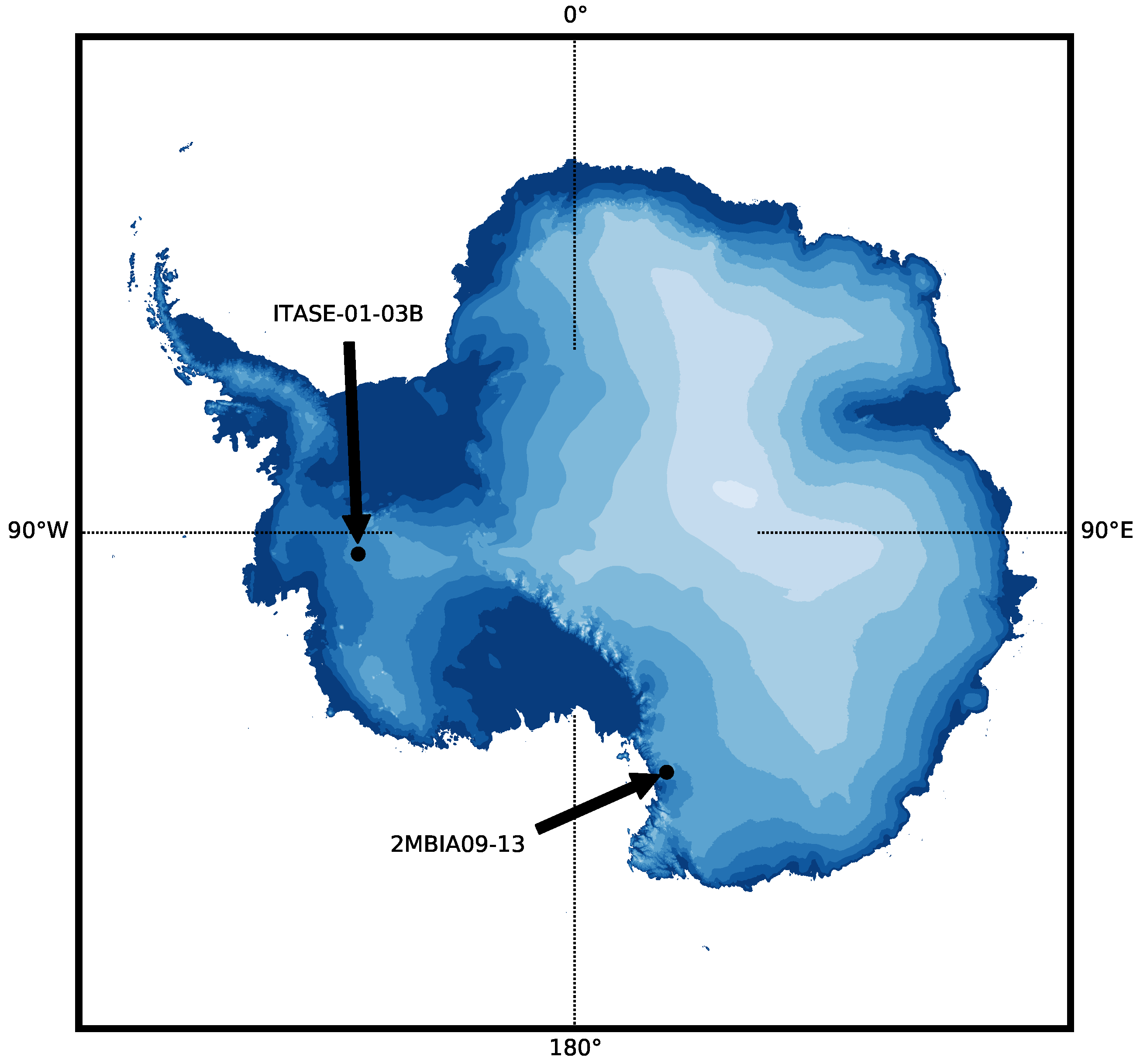
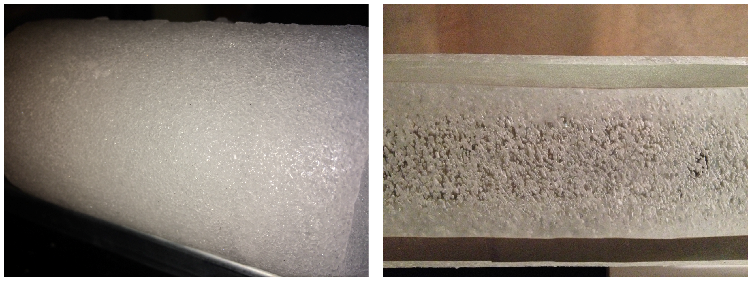
Figure 4.
Left: The annual layering in the firn ITASE core (8 cm diameter) cannot be detected visually. Right: Image of 2MBIA09 ice core that was analyzed using the laser ultrasonic acquisition system (optical tape is the gray strip). No annual layering is visible in the ice core (8 cm diameter). The layers are estimated to dip at ∼17 from horizontal.

Figure 5.
Raw ultrasonic data recorded along a section of the ITASE firn core. Each vertical line is a trace, composed of 128 repeated measurements averaged together. There is one obvious tape decoupling near 69.78 m. The arrival around 25 s is the direct P-wave. The dipping arrivals near 69.8 m are reflections from the edge of the core. The later arrivals P-wave reflections, shear waves and surface waves.
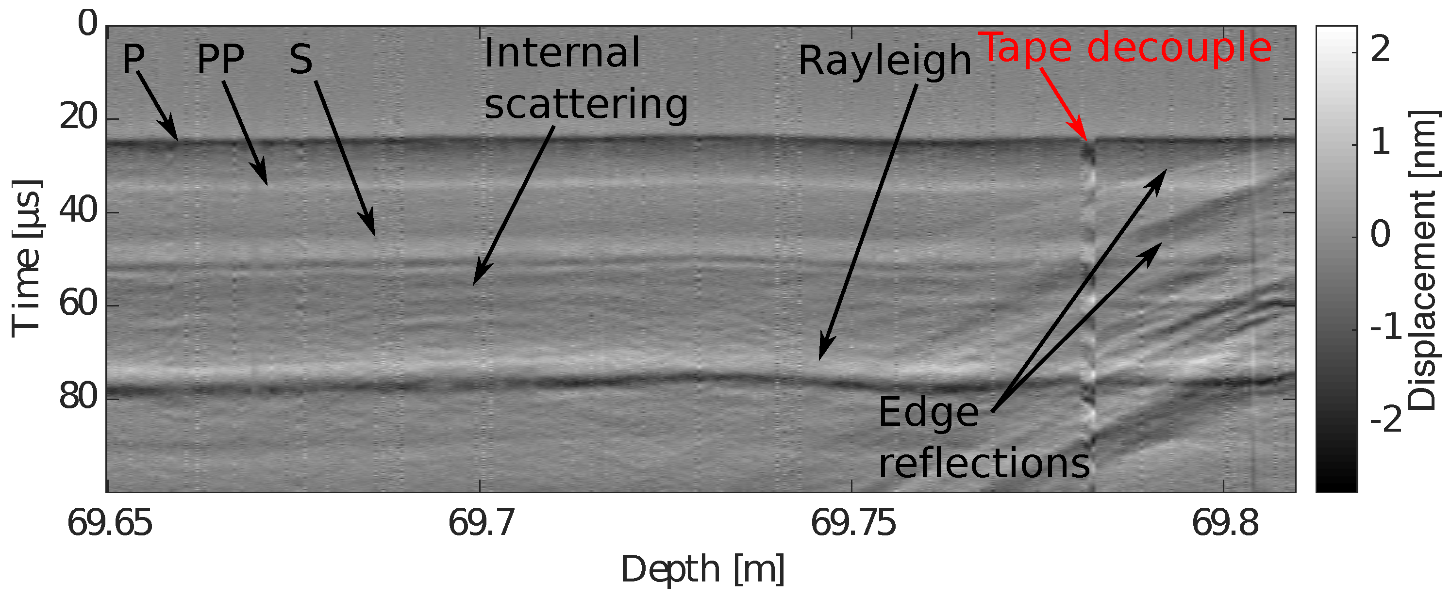
Figure 6.
Ultrasonic P-wave data between 15 and 35 s recorded on the ITASE ice core. A bandpass filter from 1 kHz to 1000 kHz has been applied. The red line indicates the P-wave arrival time automatically picked by the modified energy ratio (MER) method.
Figure 6.
Ultrasonic P-wave data between 15 and 35 s recorded on the ITASE ice core. A bandpass filter from 1 kHz to 1000 kHz has been applied. The red line indicates the P-wave arrival time automatically picked by the modified energy ratio (MER) method.
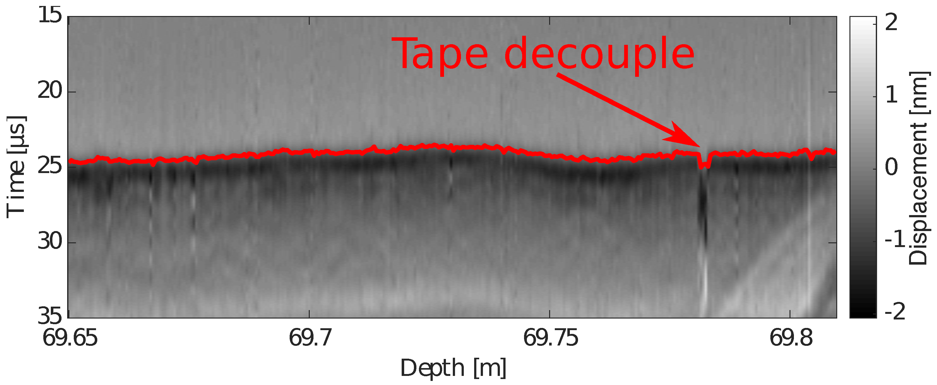
Figure 7.
Chemistry and ultrasonic P-wave velocity data from the ITASE core. Green vertical bar indicates the boundary at 1860–1861 AD.
Figure 7.
Chemistry and ultrasonic P-wave velocity data from the ITASE core. Green vertical bar indicates the boundary at 1860–1861 AD.

Figure 8.
Raw ultrasonic data recorded along a section of the 2MBIA09-13 core.
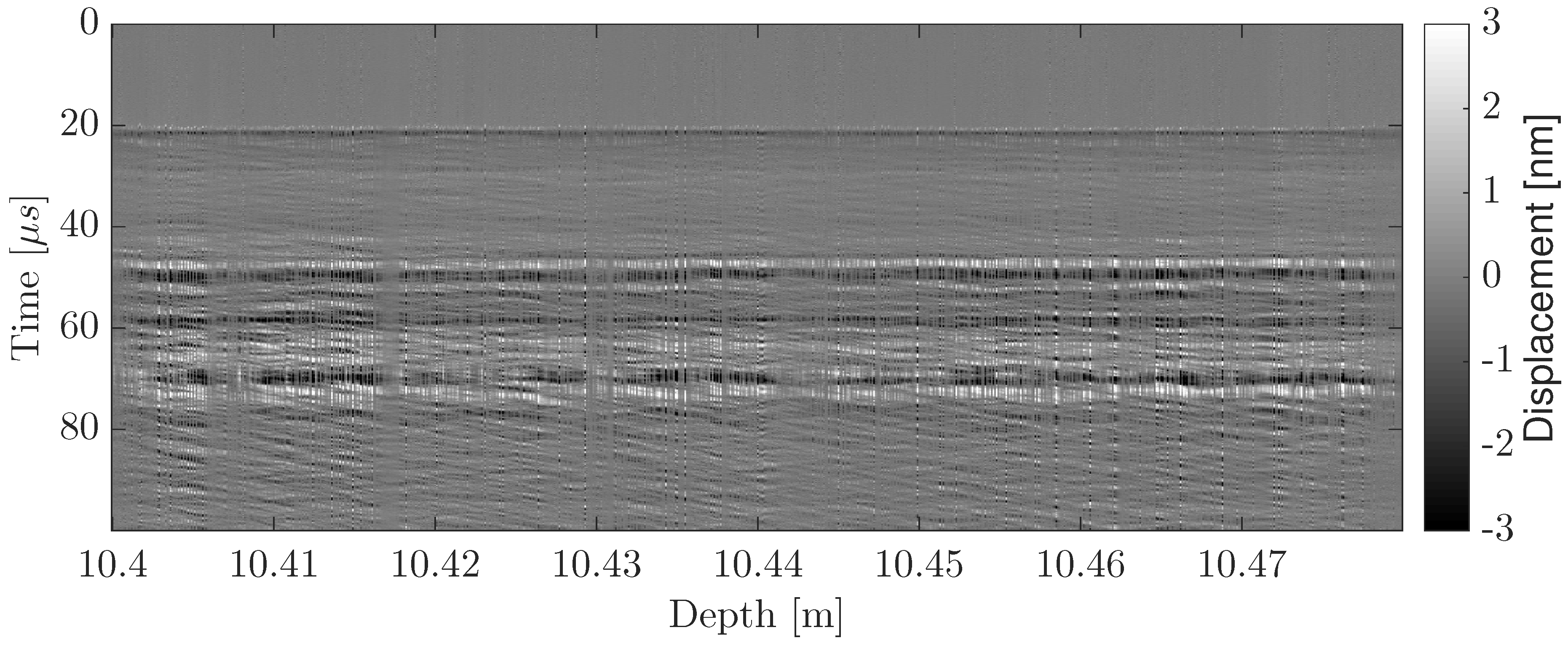
Figure 9.
Processed ultrasonic data recorded along a section of the 2MBIA09-13 core. We applied a bandpass filter from 1 kHz to 250 kHz and normalized each trace by its maximum amplitude.
Figure 9.
Processed ultrasonic data recorded along a section of the 2MBIA09-13 core. We applied a bandpass filter from 1 kHz to 250 kHz and normalized each trace by its maximum amplitude.
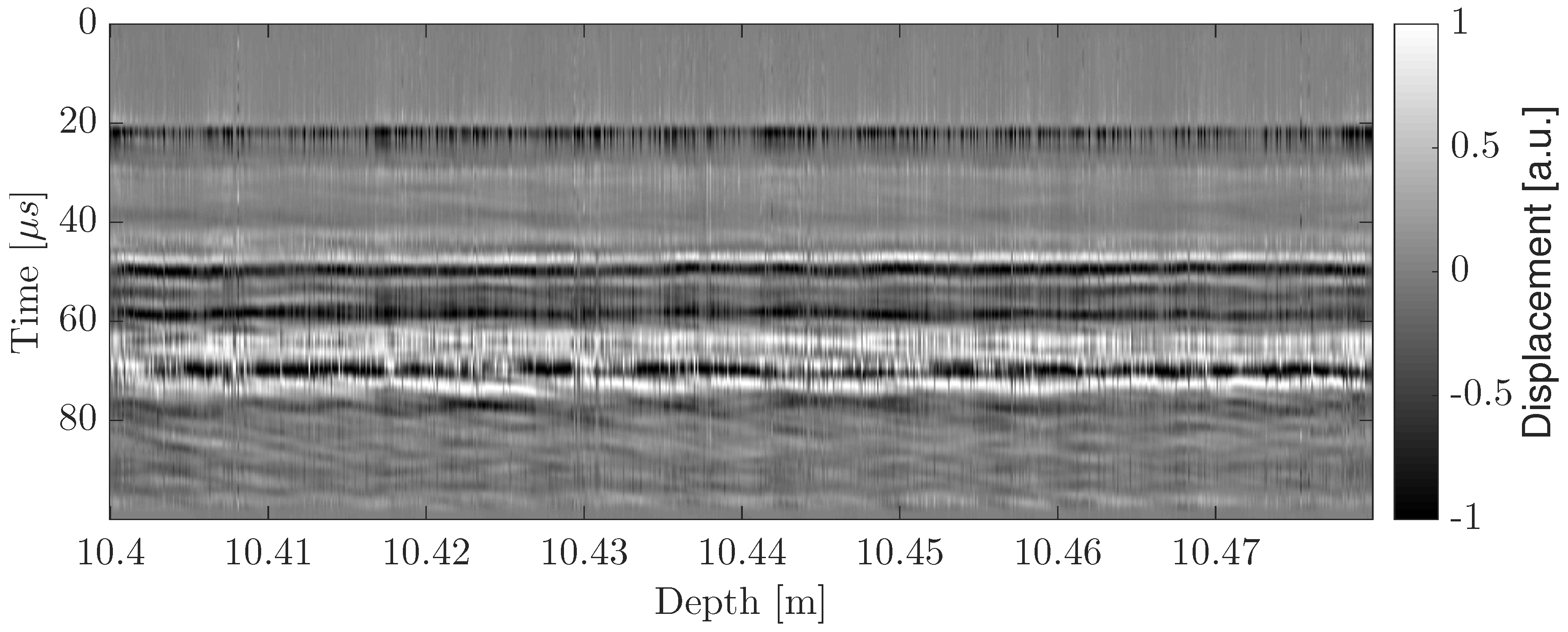
Figure 10.
Time lag estimates from cross-correlating all traces with the first trace (i.e., the trace at 10.4 cm). Top: raw time lags with a best-fit linear slope. We see increasingly negative time differences as we go to greater depth, indicating that the velocity increases with depth. Bottom: best-fit sine function to the time lags after removing the linear trend. The period of this best fit sine function is 1.97 cm.
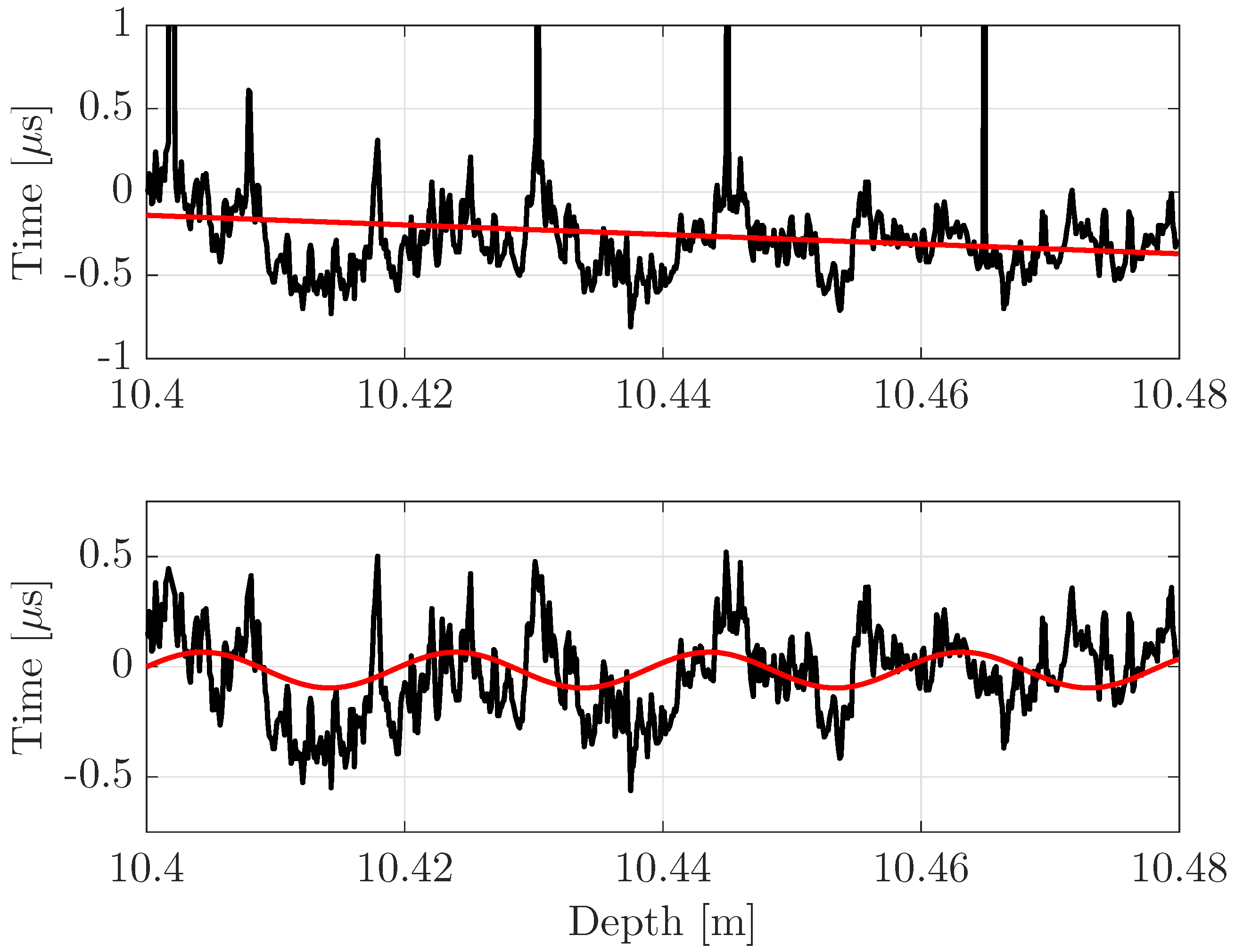
Figure 11.
Left: Rotational scan of core 2MBIA09-13. We mute three bad traces due to poor coupling between the tape and the ice surface. Right: The characteristic travel time anisotropy due to dipping layers. The red curve is the best fit to the observed Rayleigh wave velocity anisotropy.
Figure 11.
Left: Rotational scan of core 2MBIA09-13. We mute three bad traces due to poor coupling between the tape and the ice surface. Right: The characteristic travel time anisotropy due to dipping layers. The red curve is the best fit to the observed Rayleigh wave velocity anisotropy.

Table 1.
List of laser and acquisition system parameters.
| Component | Property | Value |
|---|---|---|
| Cold room | temperature | −20 ± 0.1 C |
| Vu-Port (sapphire) window | thickness | 2.5 cm |
| Source laser | laser | Nd:YAG (yttrium aluminum garnet) |
| Source laser | wavelength | 1064 nm |
| Source laser | pulse duration | 10 ns |
| Source laser | pulse energy | 0.3 J |
| Receiver laser | laser | HeNe |
| Receiver laser | wavelength | 633 nm |
| PCI oscilloscope card | precision | 16-bit |
| PCI oscilloscope card | sample rate | samples per second |
© 2017 by the authors. Licensee MDPI, Basel, Switzerland. This article is an open access article distributed under the terms and conditions of the Creative Commons Attribution (CC BY) license (http://creativecommons.org/licenses/by/4.0/).
Share and Cite
MDPI and ACS Style
Mikesell, T.D.; Van Wijk, K.; Otheim, L.T.; Marshall, H.-P.; Kurbatov, A. Laser Ultrasound Observations of Mechanical Property Variations in Ice Cores. Geosciences 2017, 7, 47. https://doi.org/10.3390/geosciences7030047
AMA Style
Mikesell TD, Van Wijk K, Otheim LT, Marshall H-P, Kurbatov A. Laser Ultrasound Observations of Mechanical Property Variations in Ice Cores. Geosciences. 2017; 7(3):47. https://doi.org/10.3390/geosciences7030047
Chicago/Turabian StyleMikesell, Thomas Dylan, Kasper Van Wijk, Larry Thomas Otheim, Hans-Peter Marshall, and Andrei Kurbatov. 2017. "Laser Ultrasound Observations of Mechanical Property Variations in Ice Cores" Geosciences 7, no. 3: 47. https://doi.org/10.3390/geosciences7030047
Note that from the first issue of 2016, this journal uses article numbers instead of page numbers. See further details here.