Article

Sewage-Borne Ammonium at a River Bank Filtration Site in Central Delhi, India: Simplified Flow and Reactive Transport Modeling to Support Decision-Making about Water Management Strategies

1
Federal Institute for Geosciences and Natural Resources (BGR) Stilleweg 2, 30655 Hannover, Germany
2
Freie Universität Berlin, Hydrogeology Group, Malteserstr. 74-100, 12249 Berlin, Germany
*
Author to whom correspondence should be addressed.
Geosciences 2017, 7(3), 48; https://doi.org/10.3390/geosciences7030048
Submission received: 26 January 2017 / Revised: 10 June 2017 / Accepted: 21 June 2017 / Published: 25 June 2017

Abstract

:
In the Indian metropolis of Delhi, the Yamuna River is highly influenced by sewage water, which has led to elevated ammonium (NH4+) concentrations up to 20 mg/L in the river water during 2012–2013. Large drinking water production wells located in the alluvial aquifer draw high shares of bank filtrate. Due to the infiltrating river water, the raw water NH4+ concentrations in some wells exceed the threshold value of 0.5 mg/L ammonia-N of the Indian drinking water specifications, making the water unfit for human consumption without prior treatment. However, to meet the city’s growing water demand, it might be advantageous to consider the long-term use of the well field. This requires the development of an adapted post-treatment unit in concert with an adjusted well field management. To better understand the groundwater dynamics and contamination and decontamination times at the well field, a theoretical modeling study has been conducted. The results of 2D numerical modeling reveal that the groundwater flux beneath the river is negligible because of the aquifer and river geometry, indicating that infiltrating river water is not diluted by the ambient groundwater. Increasing the water abstraction in the wells closest to the river would result in a larger share of bank filtrate and a decreasing groundwater table decline. Simplified 1D reactive transport models set up for a distance of 500 m (transect from the riverbank to the first production well) showed that the NH4+ contamination will prevail for the coming decades. Different lithological units of the aquifer (sand and kankar—a sediment containing calcareous nodules) have a strong influence on the respective contamination and decontamination periods, as the retardation of NH4+ is higher in the kankar than in the sand layer. Although this simplified approach does not allow for a quantification of processes, it can support decision-making about a possible future use of the well field and point to associated research needs.

1. Introduction

The urban agglomeration of Delhi, which comprises the National Capital Territory (NCT) of Delhi as well as the contiguous cities, is the second largest urban agglomeration in the world after Tokyo [1]. It is expected to further grow from 22 million inhabitants in 2011 to 31 million inhabitants in the year 2021 [2]. Associated changes in land use (Figure 1) and the increasing water demand of the fast growing population lead to a decrease in groundwater recharge and higher groundwater abstraction, causing declining groundwater tables and changing groundwater flow patterns. This poses big challenges for the city’s water management.
The enhanced use of bank filtration along the Yamuna River might be one measure to help ensure a sustainable water supply for the coming decades. Bank filtration is a technique that induces the infiltration of surface water into the aquifer by strategically constructing wells parallel to surface water bodies. In many European cities this technique is used for drinking water production, e.g., in Berlin [3] and Düsseldorf [4], Germany, and Vienna, Austria [5]. Besides reducing turbidity, it can help to remove algal toxins [6], bulk dissolved organic carbon [7], and microorganisms [8,9] from the surface water during the underground passage. However, despite those advantages, many challenges are associated with the use of this technique in Delhi as the 22 km long section of the Yamuna River within the city is strongly polluted due to the massive discharge of untreated sewage water [10,11].
To understand the effects of the highly sewage contaminated source water, a well field on the floodplain in central Delhi was extensively studied between 2008 and 2013 (e.g., [9,12,13,14]). At the well field, elevated NH4+ concentrations were measured in several hand pumps (up to 35 mg/L) and in the production well located closest to the river (up to 8 mg/L). Field data and laboratory studies revealed that the main source of the NH4+ is infiltrating sewage-influenced water from the Yamuna River [15] and that agricultural activities on the floodplain do not significantly contribute to the contamination [14].
Yet crucial questions concerning the cause and development of NH4+ concentrations at the field site remain unanswered. The mixing of infiltrating NH4+-rich river water with ambient groundwater would lead to dilution, an effect that could be used to control NH4+ concentrations in the well field by adjusting pumping schemes. However, if dilution actually occurs in the aquifer, the high groundwater NH4+ concentrations cannot result from infiltrating river water alone, meaning that another NH4+ source must be active within the aquifer. However, the groundwater flow patterns are not fully understood. For instance, on the western bank the topography rises towards the west from 204 m a.s.l. to 240 m a.s.l. at the Delhi Ridge, where quartzitic bedrock crops out [21]. It is generally assumed that the ridge functions as a groundwater recharge structure [22]. However, the decline in groundwater levels in the past few decades is especially severe in the ridge area, although most severe in the southern part [18,23]. Therefore, two scenarios are possible. Losing stream conditions were assumed by some [24], while gaining stream conditions were reported by others [18]. On the eastern bank similar uncertainty about the groundwater flow direction exists.
Simple numerical models can help to estimate the influence of different groundwater flow conditions in the well field and identify the data gaps for further research. The objectives of this modeling study, therefore, are (1) to investigate the possible inflow of groundwater from the western side beneath the river, and (2) to decide whether the production wells draw shares of ambient groundwater from the eastern areas of the floodplain where the groundwater NH4+ concentrations were reported to be low [15]. Using the model outputs, it is possible to (3) evaluate the results of two 1D reactive transport models, which were set-up to obtain an understanding of the order of magnitude of the decontamination period. This is vital to be able to choose appropriate remediation or post-treatment measures. The overall purpose of this theoretical modeling study is to better understand which options are available to improve the well field management. This might motivate scientists and stakeholders to collect and share the data necessary for setting up a calibrated 3D flow and transport model, which is necessary for more detailed planning of such measures.

2. Study Site and Methods

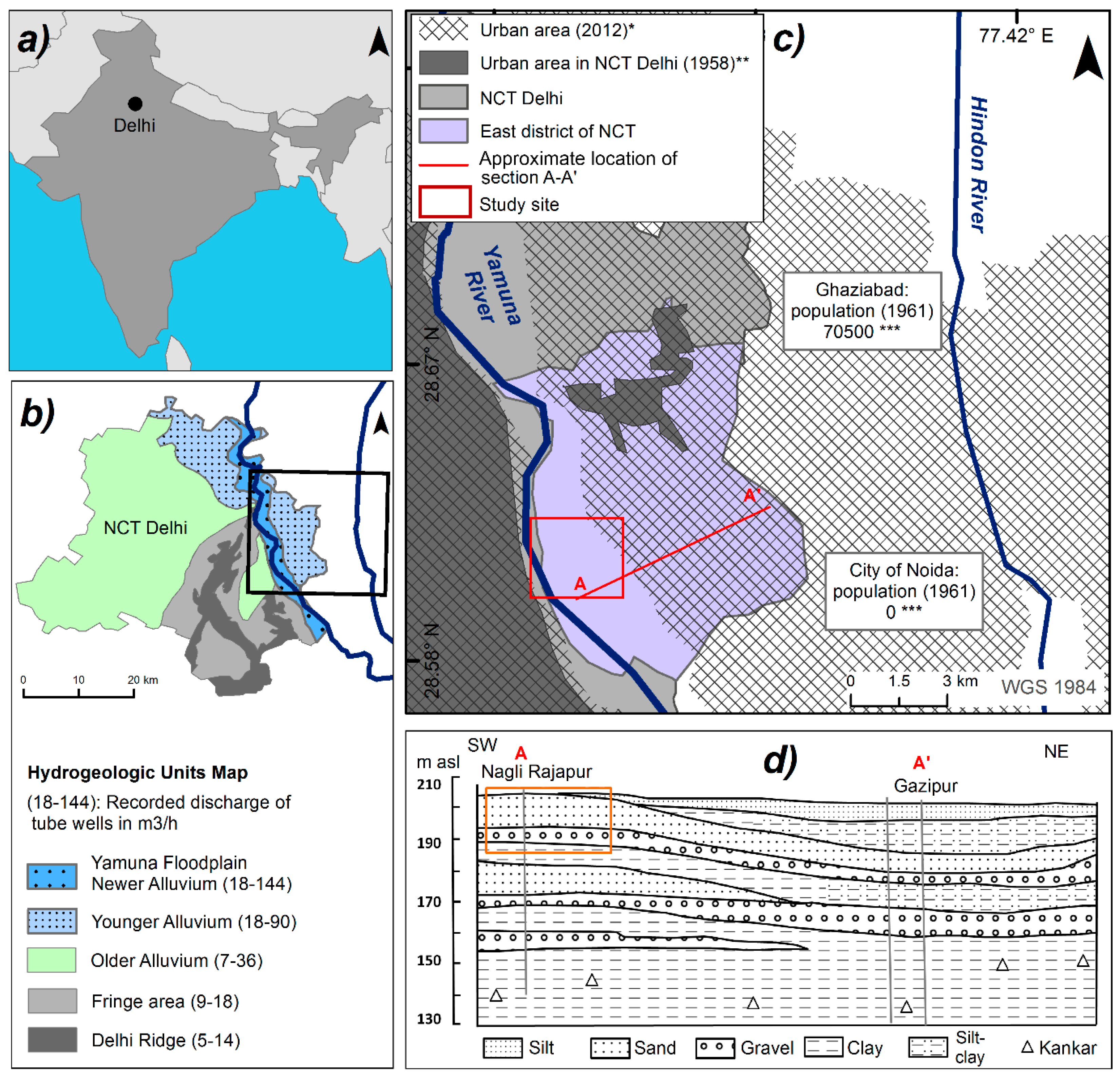
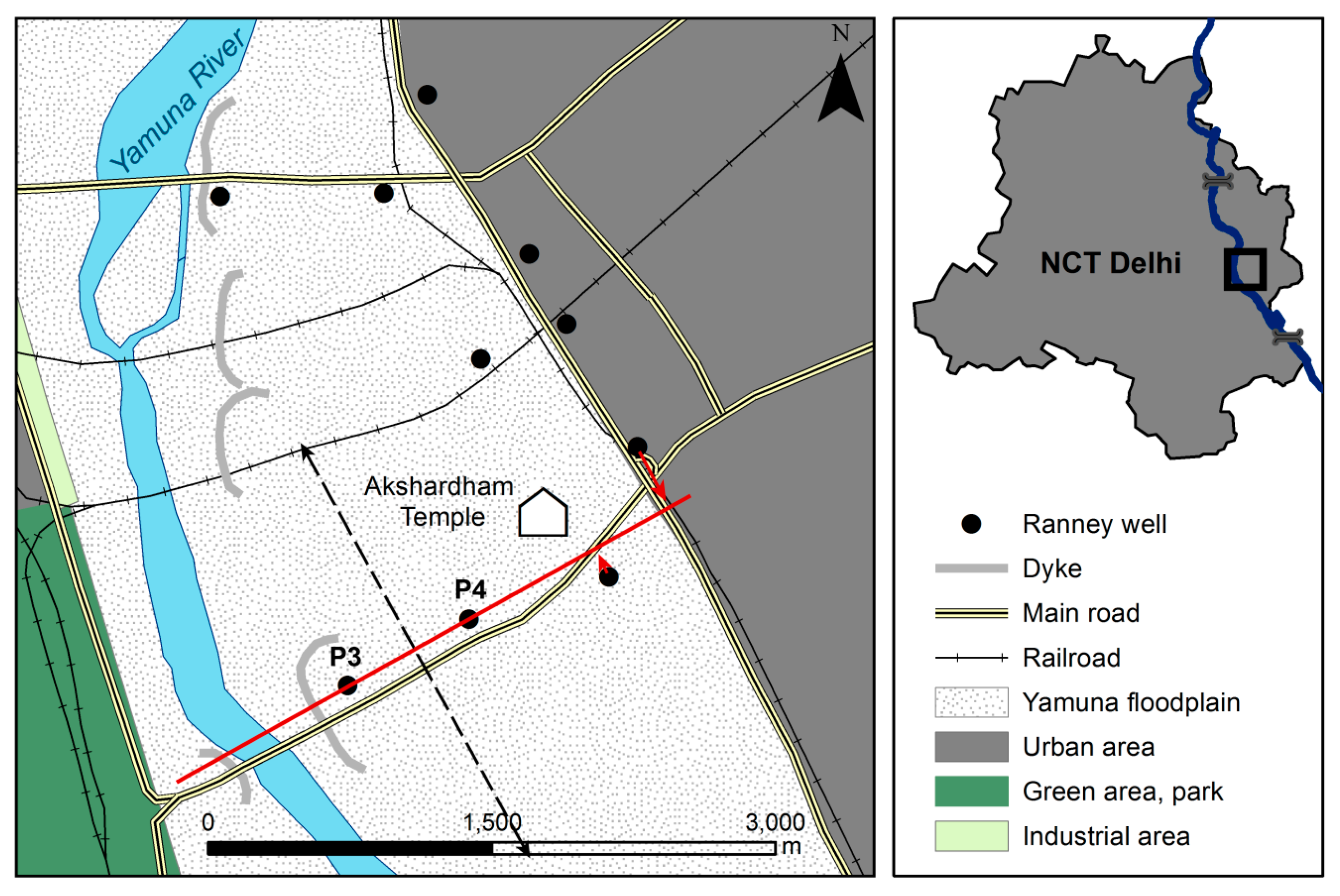
2.1. Study Area and Available Data

The study area is located on the eastern bank of the Yamuna River in central Delhi, in the district of East Delhi near the Nizamuddin Bridge and Akshardham Temple. In this area, the floodplain is asymmetrical (Figure 1b). It is narrow on the western side of the river, where the incision of the river prevented the development of a floodplain [25]. On the eastern bank, the active (undeveloped) floodplain has a width of 2.4 km. The floodplain aquifer (Newer Alluvium) is not constricted to the area of the active floodplain but extends farther east beyond the city’s boundaries, where the contact between Younger Alluvium and Older Alluvium is difficult to trace [26]. At the study site, the floodplain aquifer is between 14.5 and 16 m deep and consists of a 1 to 2 m thick kankar layer (containing gravel-sized clay-silt nodules bound by calcareous cement) overlain by medium sand. The aquifer is underlain by a thick clay layer of the Older Alluvium.
Studies conducted within the study area in the frame of the research project TECHNEAU 2006–10 were focused on a 100 m wide area along the eastern riverbank. Further studies conducted in the research project SAPH PANI aimed at making an assessment of the NH4+ contamination. Here, and especially a 500 m wide area along the river, was intensely studied. Six 8 m to 27 m deep drillings were conducted, and 13 surface- and 69 groundwater samples from a total of 14 locations were collected during seven field campaigns (2012–2013). The available data remains scarce for the area further away from the river. However, data from the Central Groundwater Board (CGWB) [20] suggest that the geological set-up can be found across the entire field site (Figure 1d). The bore logs from the study site [15] show good agreement with the CGWB cross section, assuming that the gravel layer shown in Figure 1d and the kankar layer in this study represent the same geological units. This seems to be likely as the kankar layer contains real gravel particles as well as gravel-sized nodules.

2.2. Model Set-Up

Four steady state flow simulations were modeled in 2D to test the effects of different boundary conditions and pumping schemes on the groundwater flow regime at the well field. The flow scenarios were simulated with MODFLOW 2000 [27] using the 3D interface ipht3d version 2 [28]. The steady state assumption implies that no change in storage occurs in the model and that the total inflow of water through recharge (infiltrating river water, precipitation, constant head model boundary) equals the total flow out of the model. Although this does not reflect the seasonal fluctuations in groundwater levels and groundwater recharge between the monsoon and non-monsoon time, this simplification is reasonable because no significant long-term decline in groundwater levels has been observed in the floodplain aquifer [23].
The initial 2D flow models were set up as E–W vertical cross sections with a total length of 3100 m (x-direction) and a depth of 17 m (z-direction). The model domain reaches from 400 m west of the Yamuna River to 100 m east of the undeveloped floodplain (Figure 2). To exclude influences from the upstream transect of production wells, the model width (y-direction) was set to 2600 m. This is half the distance to the upstream production wells multiplied by two because the cone of depression also spreads to the southern part of the well field. Grid spacing was set to 4 m in the x-direction and 0.2 m in the z-direction. To check for numerical errors caused by long linear cells, all models were also run with a grid length of 2 m in the x-direction.
The different lithologies found at the field site were incorporated into the model by defining zones of different hydraulic conductivities, representing the sand, kankar, and silt-clay. For the sand, an average hydraulic conductivity of 25 m/d derived from the grain size distribution [15] was chosen as the horizontal hydraulic conductivity. The average hydraulic conductivity determined by constant head permeameter tests was 3.6 m/d and this value was used as the vertical hydraulic conductivity in the models. Because of the method of sampling (only disturbed samples were available because the drilling was conducted by manual auger drilling) the results of such permeameter tests—by nature—are inaccurate. Nevertheless, the orientation of mica minerals in the sand columns perpendicular to the flow direction strongly indicate that (1) there must be a significant difference between the horizontal and vertical hydraulic conductivity and (2) the permeameter tests more closely represent the vertical hydraulic conductivity. For the kankar, hydraulic conductivities were also derived from grain size distribution curves [29] (average 315 m/d) and were determined by constant head permeameter tests (average 12 m/d). In this case, the large difference between both values results in a probably unrealistic anisotropy ratio of 26.3. The Beyer equation [29] is an empirical equation developed for sands and gravels. The kankar particles strongly differ in shape from regular gravel particles, which was thought to lead to an overestimation of hydraulic conductivities when applying the equation. Due to the lack of appropriate equations for sediments containing kankar, models were set up using the laboratory value as the vertical hydraulic conductivity and—owing to the lack of other information about kankar—assuming the same anisotropy ratio as determined for the sand: 6.9. This results in a horizontal hydraulic conductivity of 83 m/d.
For the silt-clay, a horizontal hydraulic conductivity of 0.86 m/d was chosen in accordance with the hydraulic conductivities determined for clayey-silty sediments from the study site [14]. To keep the models simple, only the silt-clay deposit along the west bank of the river was incorporated in the models, whereas the silt-clay layer at the top of the aquifer [14] was left out.
The river was defined as a zone of very high hydraulic conductivity (86,400 m/d). Kinzelbach and Rausch [30] used this approach for modeling a groundwater fed lake and showed that the chosen value does not have a big influence on the model solution as long as it is significantly higher than the hydraulic conductivities in the aquifer [30]. This approach does not take into account a limitation of the surface water-groundwater exchange caused by colmation layers with lower hydraulic conductivities. Because field investigations showed that no colmation layer was developed in most parts of the river, this simplification is valid for the field site. For the river, a constant head boundary was set with a head value of 202.1 m a.s.l.
Four wells with horizontal well screens of 60 m length (two 30 m laterals) were placed in the kankar layer. The wells are located at distances of 500, 1200, 1900, and 2400 m from the eastern riverbank. Since only steady state simulations were made, no specific temporal discretization or storage terms were necessary for solution [31]. Figure 3 depicts the river geometry and the spatial distribution of the different zones. The parameters are summarized in Table 1. For the simulations, the default values implemented in ipht3d were used, with the exception of the head change and residual criterion (HCLOSE and RCLOSE) which were set to 0.005 m and 0.005 m3/d, respectively.

2.3. Model Scenarios

To estimate the influence of different hydraulic head values at the western model boundary, two scenarios were modeled. The given hydraulic head values led to gaining stream conditions (model 1) and losing stream conditions (model 2) on the western riverbank. This was done to determine whether a share of ambient groundwater from the west side can be expected to mix with the infiltrating river water along the flow path towards the Ranney well P3. In model 1, a constant head boundary with a constant head value of 202.5 m a.s.l (0.4 m above the river water level) was defined as the western model boundary. The boundary flux at the eastern model boundary was set to a constant 1000 m3/d. Because no data is available about the conditions at the eastern model boundary, this was chosen as the best approximation. Pumping rates of 1000 m3/d were assigned to each of the four wells. In model 2, a constant head boundary with a head value of 201.1 m a.s.l. was defined as the western model boundary, which is one meter below the constant river level. The boundary flux at the eastern model boundary was again set to 1000 m3/d and the pumping rates of the wells remained at 1000 m3/d.
To demonstrate the effects of constant head versus constant flux conditions at the eastern model boundary, two further scenarios were run (models 3 and 4). To simplify the water budget calculations of the models, the set-up was modified. The western bank of the river was discarded, so that the models only comprise the part of the river where losing stream conditions prevail (Table 2). In both cases (models 3 and 4), the western model boundary was defined by a constant head of 202.1 m a.s.l. in the river. In model 3, a boundary flux of 1000 m3/d was set at the eastern model boundary. In model 4, a constant head boundary with a head value of 196 m a.s.l. was defined at the eastern model border. Because the influence of the different boundary conditions on the model results can only be seen at different abstraction rates, different model runs were performed. First, both models (3 and 4) were run with abstraction rates of 1000 m3/d per well. Secondly, the pumping rates in all wells were increased to 1200 m3/d and in the third step to 1400 m3/d per well. Hydraulic heads and water balances were compared.
Additionally, the impact of different wells on the water level decline in the eastern floodplain was tested using model 3 (constant flux boundary condition at the eastern border). This was done by firstly increasing the pumping rate first of well P3 to 1800 m3/d and 2600 m3/d while the pumping rates in all of the other wells remained at 1000 m3/d. Next, P3 was set back to 1000 m3/d and the pumping rates only in well P4 were increased to 1800 and 2600 m3/d, respectively.

2.4. Reactive Transport Modeling

Two simplified flow paths from the river to the first production well P3 were modeled with PHREEQC v3 [32]. One flow path comprises 500 m, set up as a column divided into 278 cells with a cell length of 1.8 m each. Initially, the time step in both models was set to 2 d, resulting in the average linear velocity of 0.9 m/d which was previously reported for the field site [33]. Transport parameters (effective porosities, number of exchange sites, and selectivity coefficients for the cation exchange) were determined through column experiments [34] and were used without any further adjustments (Table 3). Because of a lack of field data, dispersivities derived from the column experiments were adjusted to the model length, even though dispersion is generally higher at the field scale than at the laboratory scale due to sediment inhomogeneities which are not present in laboratory columns [35]. The longitudinal dispersivity was set to 5 m (1/100 of the flow path) in the sand and to 50 m (1/10 of the flow path) in the kankar. Because the sediment is carbonatic [36] and most water samples at the field site were slightly oversaturated with calcite, calcite was included as an equilibrium phase in the model. To check for numerical errors, all models were also run with 139 cells (3.6 m cell lengths) and 4 d time steps and selected models with 556 cells (0.9 m cell lengths) and 1 d time steps.
To model the adsorption of NH4+ in the aquifer, initial conditions in the aquifer were created by equilibrating all cells with the composition of water samples taken from a region of the aquifer still uninfluenced by the NH4+ plume [37] (Table 4). Different equilibrating solutions, charge-balanced with HCO3 before the model runs, were used for the sand and the kankar layers because groundwater-aquifer interactions in the two lithologies lead to the evolution of differing water compositions. The cells were then flushed with a displacing solution with the composition of a river water sample taken at the field site in December 2012 with an NH4+ concentration of 20 mg/L [15] until the 100% breakthrough of NH4+ at well P3 occurred. Such high NH4+ concentrations are common in the Delhi section of the Yamuna River during non-monsoon times. Concentrations of up to 35 mg/L [12] and 33.3 mg/L [10] were reported previously. For the desorption models, the following assumptions were made: the NH4+ plume has completely reached the well P3 and that the NH4+ distribution within the plume is homogenous at 35 mg/L NH4+ in the groundwater within the sand layer and 26 mg/L in the kankar layer. Defining different NH4+ concentrations in both layers is arbitrary and was done due to the lack of field data. While numerous groundwater samples were taken from the sand layer, only a limited number were available from the kankar layer and none of the few available samples had a matching NH4+ concentration of 35 mg/L [15]. Instead of equilibrating the kankar layer with a water sample from the sand layer, it was thought to be more realistic to choose the groundwater sample with the highest NH4+ concentrations measured in the kankar layer. Again, all cells were equilibrated: in this case with the solutions containing high NH4+ concentrations, as measured in the field. After equilibration, the cells were flushed with a displacing solution containing the composition of the river water upstream from Delhi, where the Yamuna is uninfluenced by sewage water [37] (Table 4). Because a redox disequilibrium was at times observed (the simultaneous occurrence of NH4+, NO2, and NO3 or the occurrence of NH4+ under oxidizing conditions), the amm.dat database was used, which defines NH4+ as a different component, thus decoupling it from the nitrogen system.
Because the kankar layer seemed to be the main flow path of the water due to the higher hydraulic conductivity, the effect of a higher flow velocity was tested by repeating the model run for the kankar layer with the initial conditions, but with a flow velocity of 1.8 m/d (time step of 1 d at a cell length of 1.8 m).

3. Results

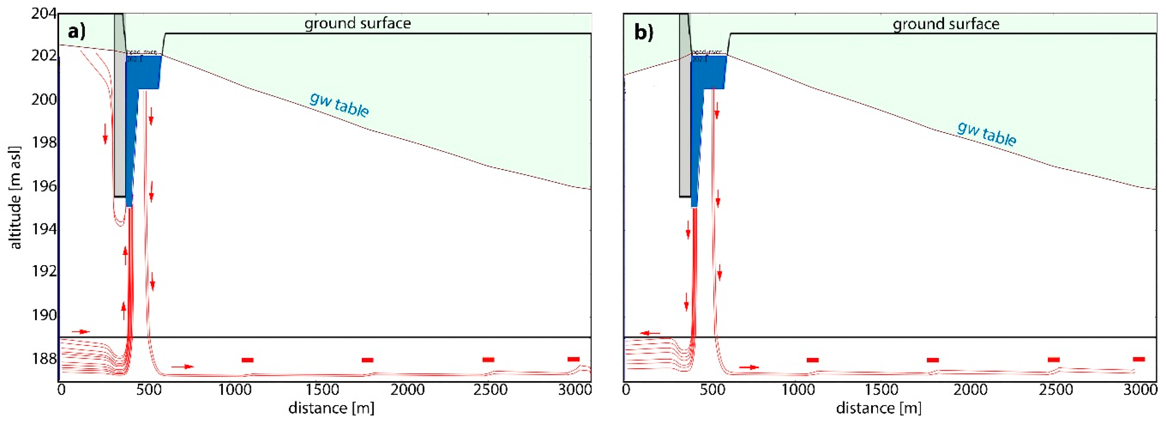
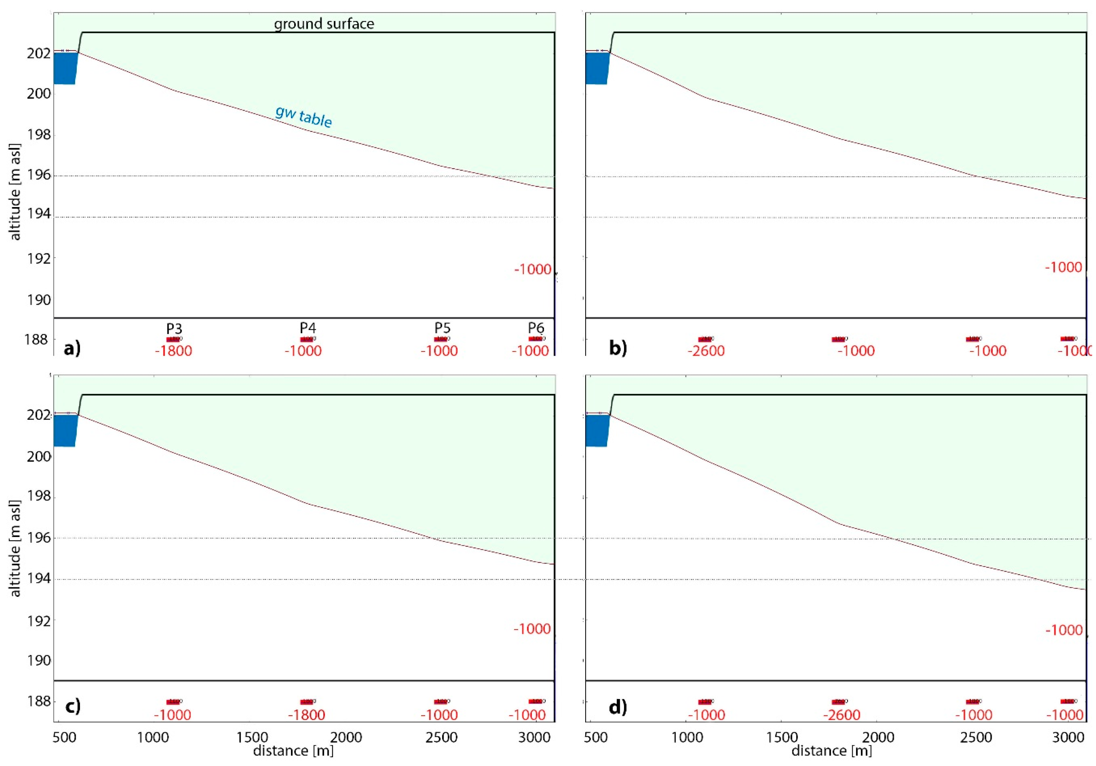
3.1. Numerical Models

The flow paths in models 1 and 2 indicate that the choice of constant head values at the western model boundary does not affect the groundwater flow at the field site on the eastern side of the river. In case of a constant head value above the river water level (model 1), gaining stream conditions prevail at the western riverbank. All groundwater from the western side (including the water from the kankar layer) infiltrates into the river and thus no groundwater flow occurs beneath the river (Figure 3a). In case of losing stream conditions at the western side of the river, the infiltrating river water flows towards the west and does not mix with the infiltrating water from the eastern side of the river (Figure 3b). In both cases the groundwater flow on the eastern side of the river is the same. Numerical errors due to cell geometry most likely did not occur: The models with a cell length of 5 m and the models with 2.5 m grid discretization in the x-direction have a very similar distribution of hydraulic heads and similar flow paths.
Models 3 and 4 demonstrate that the choice of boundary conditions has a big influence on the groundwater flow and water budget. With an initial pumping rate of 1000 m3/d per well, models 3 and 4 have similar hydraulic head distributions. Increasing the pumping rates to 1200 m3/d and subsequently to 1400 m3/d in each well led to a declining groundwater table in model 3 and to a decreasing outwards flux at the eastern boundary in model 4 (Table 5). At the same time, the infiltration of river water was higher in model 3 than in model 4. With a constant head boundary at the eastern border (model 4), increasing pumping rates further would induce an inward flux. Increasing the pumping rates of wells P3 and P4 individually showed that the water table decline is significantly smaller if higher abstraction takes place near the river in well P3 (Figure 4, Table 5).

3.2. Reactive Transport Models

Assuming the same average linear velocity of 0.9 m/d in both the sand and the kankar, it took about 15 years to reach 100% NH4+ breakthrough in the sand layer and 62 years to reach 100% NH4+ breakthrough in the kankar layer. The 50% breakthrough was reached after 10 years in the sand and after 18.5 years in the kankar layer (Figure 5). In the desorption models, the NH4+ concentrations were below the drinking water limit value of 0.5 mg/L after about 19 years in the sand layer and after about 61 years in the kankar layer (Figure 5). This is due to the higher number of exchange sites in the kankar and to different selectivity coefficients in both materials. If a flow velocity of 1.8 m/d is assumed in the kankar layer, the plume would reach well P3 about twice as fast and 100% breakthrough would occur after 31 years (50% breakthrough after 9 years). The decontamination time would also be reduced and it would only take 31 years to reach NH4+ concentrations below 0.5 mg/L.

4. Discussion

The available data about the central Delhi floodplain aquifer at the studied well field are not sufficient to set up a meaningful groundwater flow and transport model of the well field. Nevertheless, simple groundwater flow and reactive transport models can improve the understanding of the contamination and identify knowledge gaps which need to be closed before being able to develop an adapted groundwater management plan.

4.1. Flow Modeling

Simple 2D MODFLOW [27] models indicate that the hydrochemical evolution of the infiltrating river water along the flow paths (to a large portion within the kankar, to some extent in the sand) is not influenced by mixing with ambient groundwater from the western shore. This clearly answers the question about a possible western model boundary in a full-scale flow model. However, the choice of boundary conditions at the eastern model boundary, groundwater recharge rates, hydraulic conductivities, and infiltration rates still remain ambiguous.
On the eastern bank of the river, there is no rise in topography. In the 1980s, gaining stream conditions prevailed in this area with a groundwater flow direction towards the southwest [21]. However, the extremely high population growth in East Delhi and the neighboring cities of Ghaziabad and Noida (Figure 1d) probably led to changes in the groundwater flow regime. Because of the common use of private bore wells, groundwater abstraction can be assumed to be very high in the urban areas east of the floodplain. Furthermore, many large production wells are located at the border of the active floodplain (Figure 2). This most likely results in losing stream conditions and groundwater flow towards the east or southeast [18]. This was confirmed during the field campaigns, where losing stream conditions were observed [15]. However, water level measurements were restricted to sampling points near the river and no data from the eastern model area was available for this study. Nevertheless, a constant flux out of the model boundary is probably the most realistic boundary condition for the eastern model border. Although it is challenging to determine a realistic flux, this option eliminates the problem of unintentionally creating a recharge zone at the eastern model boundary when implementing too high pumping rates on the floodplain.
An average annual recharge of 74 mm (corresponding to 0.0002 m/d) was incorporated in the models. This average recharge rate was derived from the annually replenishable groundwater resources, which were reported for the Delhi floodplain and calculated using the average post-monsoon water level rise in the floodplain [38]. This rate includes recharge from precipitation, flooding, and increased infiltration due to high river water levels. Because it does not take into account the groundwater abstraction, which also takes place during the monsoon period, it should be considered as a conservative estimate. Nevertheless, the rate lies well within the range of groundwater recharge rates determined for different monsoon-influenced sites, between 24 and 198 mm or 4% and 20% of the annual recharge [39] depending on the hydraulic conductivity of the surface cover. At the study site, the average annual precipitation amounts to 600–700 mm [17] resulting in a range from 24 to 140 mm groundwater recharge.
The hydraulic conductivities used in the model set-up are subject to considerable uncertainty due to the lack of data. Pumping tests were not conducted at the field site and the sediment sampling procedures did not allow for taking undisturbed samples for laboratory analysis. Therefore, hydraulic conductivities of the different zones were derived from grain size analyses and constant head permeameter tests on disturbed sediment samples. The hydraulic conductivities determined for the sand (25 and 3.6 m/d) lie well within the commonly published range for sandy sediments. An anisotropy ratio of 6.9 (horizontal to vertical hydraulic conductivity) was determined for the sand layer. This ratio is only slightly higher than the anisotropy ratio of 5 which was found in other alluvial sediments [40]. It was thought to be adequate, and therefore used in the model set-up, because the sand shows a clear anisotropy with respect to the orientation of the grains, especially the mica minerals. In the kankar, the comparison of the hydraulic conductivity derived from the grain size analyses (315 m/d) and permeameter tests (12 m/d) results in an unusually high anisotropy ratio of 26.3. This was not implemented in the model because such high anisotropy ratios were not found elsewhere in the literature. As the empirical equation by Beyer [29] was developed to calculate the hydraulic conductivities of sand and gravel, and kankar particles are shaped differently, it was assumed that the equation might not be valid for sediments containing kankar. Instead, the authors decided to determine the horizontal conductivity for the models by multiplying the vertical conductivity derived from the constant head permeameter tests by an anisotropy ratio of 6.9. Thus the true hydraulic conductivities of the sediments, especially the horizontal conductivity of the kankar layer, might be different than the ones assigned in the model.

4.2. Reactive Transport Modeling

The decontamination times in the aquifer strongly depend on the flow velocity. In the first two models, a flow velocity of 0.9 m/d [33] was implemented. However, this assumption is unrealistic if the hydraulic conductivity of the kankar layer derived from the grain-size distribution represents the true field conditions. Therefore, the effect of a higher flow velocity was tested in a further model run with the result that the decontamination time to well P3 would be reduced from 60 years to about 30 years. This shows that 1D reactive transport modeling of the flow paths are only valid if reasonable estimates of the flow velocity are known.
Furthermore, the following assumptions and simplifications were made which influence the resulting decontamination times: (1) The Source water composition (displacing solution) was kept constant, although in reality there is a seasonal variability in the river water due to monsoon–non monsoon compositions. (2) NH4+ was decoupled from the nitrogen cycle, meaning it cannot be oxidized to nitrate in the model. This would be representative of anoxic conditions in the aquifer, which by no means must prevail after an improvement of the source water quality. It can be, therefore, assumed that decontamination times most likely would be faster if redox conditions would change from anoxic to oxidizing.

4.3. Further Research Needs

To be able to develop a meaningful groundwater flow model, which is the basis for reactive transport modeling of the contaminant plume, a sufficient database is necessary. The installation of observation wells with filter screens in the sand and in the kankar layer, respectively, is recommended for a continuous monitoring of groundwater levels and quality. Groundwater data for the well field almost exclusively exists from sampling points in the proximity of the river [13,15,41]. However, the persisting uncertainties increase towards the eastern border of the well field so that a better distribution of monitoring wells will become inevitable in the future. Although it will be difficult to achieve, groundwater abstractions rates have to be determined. Because this strongly depends on the cooperation of all water users, it is useful for future projects to include a socio-economic focus to optimize the knowledge transfer and—especially in case of agricultural water use—enhance the chance of being able to install water meters.
The different hydraulic conductivities of the two layers have a large impact on groundwater flow paths and flow velocities in the two zones of the aquifer. Because the bedding of the grains cannot be reconstructed in column experiments with disturbed samples, it is highly recommended to determine the hydraulic conductivity and the dispersivity of the zones with pumping tests and field tracer tests. Because riverbed samples were taken as disturbed grab samples, the existence of a clogging layer cannot be excluded completely. Although sediment analyses showed it to be a medium-coarse grained sand with a low organic carbon content, it would be good to verify the absence of a clogging layer by undisturbed sampling because the presence or absence of a clogging layer has a big influence on the modeling results.

4.4. Implications for Groundwater Management

Simple 2D flow and 1D reactive transport models gave impressions of possible well field management strategies. However, limited data availability only allowed for qualitative results. Nevertheless, the importance of the well P3 for water production was demonstrated as it produces the lowest decline in groundwater levels in the eastern floodplain at high abstraction rates. Three different scenarios for the future use of the central Delhi well field are conceivable.
The approach that currently seems to be opted for is operating the well field as it is currently done and successively switching off wells as NH4+ concentrations rise in the raw water. This solution “buys time” as distances between the wells are long and NH4+ transport is slow. Natural attenuation, in this case nitrification, can be expected to occur to some extent, reducing NH4+ concentrations along the flow path. The potential for nitrification mostly depends on the development of the river water quality. If the city’s sewage treatment capacity increases and conditions in the Delhi section of the Yamuna river would become permanently oxidizing, conditions in the aquifer are likely to change as well, increasing the natural attenuation. Whereas water table fluctuations have very little effect on the nitrification rates as most water is transported in the kankar layer at the bottom of the aquifer. The advantages of this strategy are that no further investment would be necessary and that contaminated water would not be used for drinking water production. The disadvantage of this option is the resulting decrease in water production within the city in times of an increasing water demand. Additionally, it makes the city more vulnerable at times when the water canals and pipelines providing the city with water are sometimes blocked for reasons of protest. If abstraction rates in wells farther away from the river are increased to make up for the loss, it would result in a larger groundwater decline in the eastern part of the aquifer. Another aspect to consider is the development of the NH4+ plume. Depending on the infiltration volumes of contaminated river water and the natural attenuation rates in the aquifer, this option could lead to large-scale contamination of the aquifer.
An alternative strategy would be to operate the well field without switching off any wells, using the existing infrastructure (e.g., pipelines and treatment units) and retrofitting existing WTPs with an advanced post-treatment technology. With this strategy, the water abstraction of the well field would remain as is, and advanced post-treatment measures would have to be planned to fit the existing conditions. However, high fluctuations in NH4+ concentrations would have to be met, which could constitute a problem for biological filters because incomplete nitrification can occur due to fluctuations in feed NH4+ concentrations [42]. The alternative application of ion exchange (e.g., using zeolites [43]) would be suitable to treat the fluctuating NH4+ concentrations, but because of high space requirements this technology might be difficult to apply in the city’s large treatment plants. Other techniques seem to be unsuitable for application in Delhi due to the high NH4+ concentrations in the raw water (breakpoint chlorination [44]—which could furthermore result in the formation of undesirable by-products [45]) or—in the case of membrane filtration (e.g., reverse osmosis)—because of high investment and operating costs.
The third and most advanced option is to develop the central Delhi well field in concert with a treatment unit. A post-treatment strategy for groundwater with high NH4+ concentrations adapted to the local conditions would have to be established, e.g., some form of biological filter due to their apparent cost-efficiency and widespread application (biological granular activated carbon filters or biological rapid sand filters). At the same time, a well field management could be set up to provide the treatment facility with the required water in terms of quantity and quality, which would include the buffering of high NH4+ fluctuations through the application of adapted pumping schemes. Depending on the capacity of the planned treatment unit, it could be advantageous to increase the water production at the well field. This could be achieved by placing additional wells even closer to the river in the form of a well gallery. Compared to another large well field in the North of Delhi (Palla) where the Yamuna riverbed shifts over several 100 m per decade, the river in central Delhi stays at a relatively constant location owing to the numerous embankments. This makes well field management easier than in Palla. However, several issues have to be considered before choosing this option: (1) How much Yamuna River water can be abstracted according to the water sharing agreement with the other basin states? (2) Are there any legal issues? (3) Would this measure be socially accepted? In Delhi, the highly contaminated water of the Yamuna River is often publicly discussed. To opt for an increased use of this source should be thoughtfully explained and communicated to the public.
For all options, a calibrated and validated flow and reactive transport model of the entire well field is necessary because the expected scenarios have to be known beforehand to be able to choose the appropriate production, treatment, or remediation schemes. However, this work demonstrates the strength of the modeling approaches in the context of groundwater management in rapidly expanding megacities in emerging countries with urgent needs to provide decision support to groundwater management.

Acknowledgments

This research was done in the framework of SAPH PANI, an EU funded project about the improvement of natural water treatment systems in water stressed urban and peri—urban areas in India (EU Grant agreement no: 282911), co-funded by Veolia Eau. The authors would like to thank the Delhi Jal Board for supporting the work at the Delhi field site by giving drilling and sampling permissions. Furthermore the authors would like to thank the two anonymous reviewers for their contributions towards improving the earlier version of the manuscript.

Author Contributions

Maike Groeschke and Theresa Frommen collected the field data and performed the laboratory experiments to determine the selectivity coefficients. Michael Schneider contributed to the development of the conceptual model. Maike Groeschke and Andreas Winkler developed the reactive transport models. Maike Groeschke wrote the paper.

Conflicts of Interest

The authors declare no conflict of interest.

References

  1. United Nations. World Urbanization Prospects: The 2014 Revision, Highlights; ST/ESA/SER.A/352; UN: New York, NY, USA, 2014; Available online: http://esa.un.org/unpd/wup/Highlights/WUP2014-Highlights.pdf (accessed on 2 April 2015).
  2. National Capital Region Planning Board, Ministry of urban Develpoment (India). Draft revised regional plan 2021 National Capital Region; Ministry of Urban Development, Government of India: New Delhi, India, 2013; Available online: http://www.indiaenvironmentportal.org.in/files/file/Draft%20Revised%20Regional%20plan.pdf (accessed on 12 January 2015).
  3. Massmann, G.; Pekdeger, A.; Heberer, T.; Grützmacher, G.; Dünnbier, U.; Knappe, A.; Meyer, H.; Mechlinski, A. Drinking-Water Production in Urban Environments-Bank Filtration in Berlin. Grundwasser 2007, 12, 232–245. [Google Scholar] [CrossRef]
  4. Eckert, P.; Irmscher, R. Over 130 years of experience with Riverbank Filtration in Düsseldorf, Germany. J. Water Supply Res. Techno.—Aqua 2006, 55, 283–291. [Google Scholar]
  5. Orlikowski, D.; Weigelhofer, G.; Hein, T. The impact of river water on groundwater quality in an urban floodplain area, the Lobau in Vienna. In Proceedings of the 36th International Conference of IAD, Austrian Committee Danube Research/IAD, Vienna, Austria, 4—8 September 2006; 4, pp. 200–202. [Google Scholar]
  6. Dillon, P.J.; Miller, M.; Fallowfield, H.; Hutson, J. The potential of riverbank filtration for drinking water supplies in relation to microsystin removal in brackish aquifers. J. Hydrol. 2002, 266, 209–221. [Google Scholar] [CrossRef]
  7. Grünheid, S.; Amy, G.; Jekel, M. Removal of bulk dissolved organic carbon (DOC) and trace organic compounds by bank filtration and artificial recharge. Water Res. 2005, 39, 3219–3228. [Google Scholar] [CrossRef] [PubMed]
  8. Weiss, W.J.; Bouwer, E.J.; Aboytes, R.; LeChevallier, M.W.; O’Melia, C.R.; Le, B.T.; Schwab, K.J. Riverbank filtration for control of microorganisms: Results from field monitoring. Water Res. 2005, 39, 1990–2001. [Google Scholar] [CrossRef] [PubMed]
  9. Sprenger, C.; Lorenzen, G.; Grunert, A.; Ronghang, M.; Dizer, H.; Selinka, H.C.; Girones, R.; López-Pila, J.M.; Mittal, A.K.; Szewzyk, R. Removal of indigenous coliphages and enteric viruses during riverbank filtration from highly polluted river water in Delhi (India). J. Water Health 2014, 12, 332–342. [Google Scholar] [CrossRef] [PubMed]
  10. Central Pollution Control Board, Ministry of Environment & Forests, Government of India. Water Quality Status of Yamuna River (1999–2005); ADSORBS/41/2006–07; Central Pollution Control Board: New Delhi, India, 2006; Available online: http://www.cpcb.nic.in/newitems/11.pdf (accessed on 9 September 2014).
  11. Central Pollution Control Board, Ministry of Environment & Forests, Government of India. Status of Water Quality in India – 2012; MINARS/36 /2013–14; Central Pollution Control Board: New Delhi, India, 2013; Available online: http://www.cpcb.nic.in/WQ_Status_Report2012.pdf (accessed on 5 May 2015).
  12. Pekdeger, A.; Lorenzen, G.; Sprenger, C. Preliminary report on data of all inorganic substances and physicochemical parameters listed in the Indian and German Drinking Water Standards from surface water and groundwater at the 3 (+1) field sites; TECHNEAU Deliverable D 5.2.2.2008; European Commission: Luxembourg, 2008; Available online: https://www.techneau.org/fileadmin/files/Publications/Publications/Deliverables/D5.2.2.pdf (accessed on 24 Augest 2012).
  13. Lorenzen, G.; Sprenger, C.; Taute, T.; Pekdeger, A.; Mittal, A.; Massmann, G. Assessment of the potential for bank filtration in a water-stressed megacity (Delhi, India). Environ. Earth Sci. 2010, 61, 1419–1434. [Google Scholar] [CrossRef]
  14. Groeschke, M.; Kumar, P.; Winkler, A.; Grützmacher, G.; Schneider, M. The role of agricultural activity for ammonium contamination at a riverbank filtration site in central Delhi (India). Environ. Earth Sci. 2016, 75, 1–14. [Google Scholar] [CrossRef]
  15. Groeschke, M.; Frommen, T.; Taute, T.; Schneider, M. The impact of sewage-contaminated river water on groundwater ammonium and arsenic concentrations at a riverbank filtration site in central Delhi, India. Hydrogeol. J. 2017, 1–13. [Google Scholar] [CrossRef]
  16. Central Ground Water Board (CGWB), Ministry of Water Resources, Government of India. Groundwater Yearbook 2011–12, National Capital Territory Delhi. Central Ground Water Board; CGWB: New Delhi, India, 2012.
  17. Central Ground Water Board (CGWB), Ministry of Water Resources, Government of India. Hydrogeological Framework and Ground Water Management Plan of NCT Delhi; CGWB: New Delhi, India, 2006.
  18. Kumar, M.; Rao, M.S.; Kumar, B.; Ramanathan, A. Identification of aquifer-recharge zones and sources in an urban development area (Delhi, India), by correlating isotopic tracers with hydrological features. Hydrogeol. J. 2011, 19, 463–474. [Google Scholar] [CrossRef]
  19. Town and Country Planning Organisation, Ministry of Urban Development, Government of India. Evaluation study of DMA towns in National Capital Region (NCR); Government of India: New Delhi, India, 2007. Available online: http://tcpomud.gov.in/divisions/mutp/dma/final_dma_report.pdf (accessed on 2 April 2015).
  20. Central Ground Water Board (CGWB), Ministry of Water Resources, Government of India. Ground Water Information Booklet of East District, NCT, Delhi; CGWB: New Delhi, India, 2013. Available online: http://cgwb.gov.in/District_Profile/Delhi/East.pdf (accessed on 21 September 2015).
  21. Das, B.K.; Kakar, Y.P.; Moser, H.; Stichler, W. Deuterium and oxygen-18 studies in groundwater of the Delhi area, India. J. Hydrol. 1988, 98, 133–146. [Google Scholar] [CrossRef]
  22. Chatterjee, R.; Gupta, B.; Mohiddin, S.; Singh, P.; Shekhar, S.; Purohit, R. Dynamic groundwater resources of National Capital Territory, Delhi: assessment, development and management options. Environ. Earth Sci. 2009, 59, 669–686. [Google Scholar] [CrossRef]
  23. Central Ground Water Board (CGWB), Ministry of Water Resources, Government of India. Ground Water Yearbook 2005–2006. National Capital Territory Delhi; CGWB: New Delhi, India, 2006.
  24. Sprenger, C. Technical report—Numerical modelling of surface-/groundwater interactions at the flood plain in Delhi (India). SAPH PANI Project report. 2013; (unpublished). [Google Scholar]
  25. Sinha, R.; Jain, V.; Babu, G.P.; Ghosh, S. Geomorphic characterization and diversity of the fluvial systems of the Gangetic Plains. Geomorphology 2005, 70, 207–225. [Google Scholar] [CrossRef]
  26. Kazim, M.K.; Kumar, R.; Kumar, H.; Gupta, A.K.; Bagchi, J.; Srivastava, S.S. Geological and geomorphological mapping of NCT Delhi on 1:10,000 scale; Field Season 2005–06, 2006–07 and 2007–08; Geological Survey of India: New Delhi, India, 2008. [Google Scholar]
  27. Harbaugh, A.W.; Banta, E.R.; Hill, M.C.; McDonald, M.G. MODFLOW-2000, the U.S. Geological Survey Modular Ground-Water Model - User Guide to Modularization Concepts and the Ground-Water Flow Process; Open-File Report 00–92; USGS: Reston, VA, USA, 2000. Available online: http://pubs.er.usgs.gov/publication/ofr200092 (accessed on 16 May 2014).
  28. Atteia, O. iPht3d Manual Version 2-e 28/05/2014. 2014, p. 23. Available online: http://oatteia.usr.ensegid.fr/iPht3d/ (accessed on 4 July 2014).
  29. Beyer, W. Zur Bestimmung der Wasserdurchlässigkeit von Kiesen und Sanden aus der Kornverteilungskurve. Wasserwirtschaft Wassertechnik 1964, 14, 165–168. [Google Scholar]
  30. Kinzelbach, W.; Rausch, R. Grundwassermodellierung: eine Einführung mit Übungen; Gebrüder Borntraeger: Stuttgart, Berlin, Germany, 1995; pp. 158–161. [Google Scholar]
  31. Holtschlag, D.J.; Luukkonen, C.L.; Nichols, J.R. Simulation of Ground-Water Flow in the Saginaw Aquifer, Clinton, Eaton, and Ingham Counties, Michigan; USGS: Reston, VA, USA, 1996. Available online: http://pubs.usgs.gov/wsp/2480/report.pdf (accessed on 19 September 2015).
  32. Parkhurst, D.L.; Appelo, C.A.J. Description of Input and Examples for PHREEQC Version 3 - A Computer Program for Speciation, Batch-Reaction, One-Dimensional Transport, and Inverse Geochemical Calculations; USGS: Reston, VA, USA, 2013. Available online: http://pubs.usgs.gov/tm/06/a43/ (accessed on 9 September 2014).
  33. Sprenger, C. Surface-/groundwater interactions associated with river bank filtration in Delhi (India)—Investigation and modelling of hydraulic and hydrochemical processes. Ph.D. Thesis, Freie Universität Berlin, Berlin, Germany, 2011. [Google Scholar]
  34. Groeschke, M. Transport and Fate of Ammonium at a Riverbank Filtration Site in Delhi (India): Assessment of the Groundwater Contamination, Treatment Strategies and Recommendations for an Adapted Management. Ph.D. Thesis, Freie Universität Berlin, Berlin, Germany, 2016. [Google Scholar]
  35. Gelhar, L.W.; Welty, C.; Rehfeldt, K.R. A critical review of data on field-scale dispersion in aquifers. Water Resour. Res. 1992, 28, 1955–1974. [Google Scholar] [CrossRef]
  36. Eybing, M. Charakterisierung eines alluvialen Grundwasserleiters in Delhi (Indien): Sedimentanalysen von Bohrungen an einem Uferfiltrationsstandort am Yamuna. (Characterization of an alluvial aquifer in Delhi, India: Sediment analyses of samples from drillings at a riverbank filtration site at the Yamuna River). B.Sc. Thesis, Freie Universität Berlin, Insitute of Geological Sciences, Berlin, Germany, 2014. [Google Scholar]
  37. Groeschke, M.; Frommen, T.; Grützmacher, G.; Schneider, M.; Sehgal, D. Application of Bank Filtration in Aquifers Affected by Ammonium–The Delhi Example. In Natural Water Treatment Systems for Safe and Sustainable Water Supply in the Indian Context: Saph Pani; Wintgens, T., Anders, N., Elango, L., Asolekar, R.S., Eds.; IWA Publishing: London, UK, 2015; pp. 57–77. [Google Scholar]
  38. Shekhar, S.; Prasad, R.K. The groundwater in the Yamuna flood plain of Delhi (India) and the management options. Hydrogeol. J. 2009, 17, 1557–1560. [Google Scholar] [CrossRef]
  39. Rangarajan, R.; Athavale, R.N. Annual replenishable ground water potential of India—an estimate based on injected tritium studies. J. Hydrol. 2000, 234, 38–53. [Google Scholar] [CrossRef]
  40. Su, G.W.; Jasperse, J.; Seymour, D.; Constantz, J. Estimation of Hydraulic Conductivity in an Alluvial System Using Temperatures. Ground Water 2004, 42, 890–901. [Google Scholar] [CrossRef] [PubMed]
  41. Sprenger, C.; Lorenzen, G. Hydrogeochemistry of Urban Floodplain Aquifer Under the Influence of Contaminated River Seepage in Delhi (India). Aquat Geochem. 2014, 20, 519–543. [Google Scholar] [CrossRef]
  42. Rittmann, B.E. Analyzing Biofilm Processes Used in Biological Filtration. J. Am. Water Works Assoc. 1990, 82, 62–66. [Google Scholar] [CrossRef]
  43. Li, M.; Zhu, X.; Zhu, F.; Ren, G.; Cao, G.; Song, L. Application of modified zeolite for ammonium removal from drinking water. Desalination 2011, 271, 295–300. [Google Scholar] [CrossRef]
  44. Gauntlett, R.B. Removal of Nitrogen Compounds. In Developments in Water Treatment 2; Lewis, W.M., Ed.; Applied Science Publishers: London, UK, 1980; pp. 53–78. [Google Scholar]
  45. Takó, S.; Laky, D. Laboratory Experiments for Arsenic and Ammonium Removal—The Combination of Breakpoint Chlorination and Iron(III)-Coagulation. J. Environ. Sci. Eng. 2012, 1165–1172. [Google Scholar]
Figure 1. (a) Location of Delhi. (b) Hydrogeologic units of the National Capital Territory (NCT) of Delhi and data frame of Figure 1c (map modified after [16]). Discharge of the tube wells compiled from [16,17]. (c) Population development in the eastern part of Delhi, Ghaziabad, and Noida, and the location of the study area (red box) (* data from [2]; ** modified after [18]; *** [19]) (d) SW-NE vertical cross section through East Delhi (location shown in (c)). The orange box represents the approximate position of the study area (modified after [20]).
Geosciences 07 00048 g001
Figure 2. Overview of the study area, location of the modeled x-section (red line), and the model extent in the y-direction (dashed arrows).
Geosciences 07 00048 g002
Figure 3. (a) Model 1: Gaining stream conditions prevail in the west. Red lines: particle tracking (forward), red arrows: groundwater flow direction, red bars: well screens, grey areas: silt-clay zones. Note the different scales (in m) on the x- and z-axes. (b) Model 2: Losing stream conditions prevail in the western part of the model.
Geosciences 07 00048 g003
Figure 4. Effects of different pumping schemes on the groundwater levels. The water table decline is significantly smaller if the abstraction rates are increased in well P3 (a,b) instead of in well P4 (c,d).
Geosciences 07 00048 g004
Figure 5. (a) Results of the adsorption modeling. (b) Results of the desorption modeling.
Geosciences 07 00048 g005
Table 1. Parameters used to set up the initial 2D flow models (models 1 and 2).
ParameterValue (General)Values in Different Zones
SandKankarSilt-ClayRiver
Flow simulationSteady state------------
Aquifer typeFree------------
Simulation time (days)1000------------
Model extent column, x-direction (m)3100------------
Model extent layer, z-direction (m)17------------
Zmin (m a.s.l.)187------------
Zmax (m a.s.l.)204------------
Model thickness (y-direction) (m)2600------------
Grid spacing Δx (m)4 (2)------------
Grid spacing Δz (m)0.2------------
Horizontal hydraulic conductivity (m/d)---25830.8686,400
Vertical hydraulic conductivity (m/d)---3.6120.4386,400
Recharge (m/d)0.0002------------
Table 2. Model extent in the x-direction for models 3 and 4. All other parameters are shown in Table 1.
ParameterValue
Model extent column, x-direction (m)2625
xmin (m)475
xmax (m)3100
Number of columns525
Table 3. Transport parameters used in the 1D reactive transport models (modified after [37]).
ParameterUnitSandKankar
Effective Porosity (ne) *---0.240.175
Number of exchange sitesmeq/1 L water0.0540.21
log_kNa\K---0.980.67
log_kNa\Ca---0.180.10
log_kNa\Mg---−0.09−0.28
log_kNa\NH4---0.810.55
* Effective porosities are not explicitly included in PHREEQC [32] models. They are incorporated through the number of exchange sites.
Table 4. Adsorption and desorption modeling: Composition of the equilibrating and displacing solutions.
Para-MeterUnitAdsorption ExperimentsDesorption Experiments
Equil. Solution SandEquil. Solution KankarDisplacing SolutionEquil. Solution SandEquil. Solution KankarDisplacing Solution
T°C25.025.025.025.025.025.0
pHpH7.587.47.66.937.238.56
EhmV1601758210584268
ECµS/cm495893158816151153457
Namg/L19.967.51719779.735
Kmg/L5.46.815.417.313.29
Mgmg/L142333.738.724.814
Camg/L63.78065.4126.589.144
Femg/L0.090.10.0716.95.20.62
Mnmg/L0.090.30.30.420.270.05
HCO3mmol/L5.25.96.511.98.32.7
Clmg/L67821814111538
SO4mg/L2531255446
S2−mg/L0000.0400
NH4+mg/L00.62035260.1
NO2mg/L0.0050.030.020.0050.005--
NO3mg/L03.5000.05--
T: Temperature; Eh: Redox potential relative to the standard hydrogen electrode; EC: Electrical conductivity.
Table 5. Results of different pumping scenarios applied in models 3 and 4 (grid spacing of 2 m in the x-direction).
ModelPumping Rate (m3/d/well)Inflow (Heads) (m3/d)Recharge (m3/d)Well (out) (m3/d)Flux (out) (m3/d)HeadEast (m a.s.l.)
Model 310003699130540051000195.8
Model 312004493130547991000194.4
Model 314005299130556041000192.8
Model 41000362713054005927196
Model 41200394013054799448196
Model 414004298130556040196
Model 3P3: 1800 *4499130548051000195.3
Model 3P4: 1800 *4499130548051000194.7
Model 3P3: 2600 *5299130556051000194.8
Model 3P4: 2600 *5299130556051000193.4
* Pumping rate in all other wells is 1000 m3/d.

