Influence of Substratum Hydrophobicity on the Geomicrobiology of River Biofilm Architecture and Ecology Analyzed by CMEIAS Bioimage Informatics

Abstract

Microbial biogeography in terrestrial and freshwater ecosystems is mainly dominated by community biofilm lifestyles. Here, we describe applications of computer-assisted microscopy using CMEIAS (Center for Microbial Ecology Image Analysis System) bioimage informatics software for a comprehensive analysis of river biofilm architectures and ecology. Natural biofilms were developed for four summer days on microscope slides of plain borosilicate glass and transparent polystyrene submerged in the Red Cedar River that flows through the Michigan State University campus. Images of the biofilm communities were acquired using brightfield and phase-contrast microscopy at spatial resolutions revealing details of microcolonies and individual cells, then digitally segmented to the foreground objects of interest. Phenotypic features of their size, abundance, surface texture, contour morphology, fractal geometry, ecophysiology, and landscape/spatial ecology were digitally extracted and evaluated by many discriminating statistical tests. The results indicate that river biofilm architecture exhibits significant geospatial structure in situ, providing many insights on the strong influence that substratum hydrophobicity–wettability exert on biofilm development and ecology, including their productivity and colonization intensity, morphological diversity/dominance/conditional rarity, nutrient apportionment/uptake efficiency/utilization, allometry/metabolic activity, responses to starvation and bacteriovory stresses, spatial patterns of distribution/dispersion/connectivity, and interpolated autocorrelations of cooperative/conflicting cell–cell interactions at real-world spatial scales directly relevant to their ecological niches. The significant impact of substratum physicochemistry was revealed for biofilms during their early immature stage of development in the river ecosystem. Bioimage informatics can fill major gaps in understanding the geomicrobiology and microbial ecology of biofilms in situ when examined at spatial scales suitable for phenotypic analysis at microcolony and single-cell resolutions.

1. Introduction

This study describes applications of our software suite called the “Center for Microbial Ecology Image Analysis System” (CMEIAS) to analyze microbial biofilm assemblages derived from river bacterioplankton and colonized on microscope slides differing in hydrophobicity and surface wettability. The findings reveal that substratum physicochemistry significantly impacts on the early immature stage of biofilm community development in the river ecosystem, and that bioimage informatics can fill major gaps in understanding the phenotypic characteristics important to the geomicrobiology and ecology of biofilms analyzed in situ at microcolony and single-cell resolution.

1.1. CMEIAS Software Development

The mission of our CMEIAS project is to develop, document and release a comprehensive suite of bioimage informatics analysis software applications designed to strengthen quantitative, microscopy-based approaches for understanding microbial ecology, at spatial scales directly relevant to microbes and their ecological niches without the need for cultivation [1,2,3,4,5,6,7,8,9,10,11,12,13,14,15,16]. The wealth of information gained by CMEIAS analysis of digital images can bridge with other modern genotypic and phenotypic technologies to fill knowledge gaps revealing additional insights of in situ phenotypic characteristics of ecological importance to microbial cells, populations, communities and microbiomes. Examples include their biodiversity, productivity (conversion of available nutrient resources into biomass and metabolic energy), food-web dynamics, landscape ecology, strategies of successful colonization behavior, adaptations and resilience to environmental stresses, and intensities of interaction with each other within biofilms [2,3,4,5,6,7,8,9,10,11,12,13,14,15]. When finalized, the copyrighted CMEIAS software tools and their comprehensive documentations are released as free downloads at our project website [1]. Previously released CMEIAS software components used in this study include: (i) the dynamic library-linked extension plugins operating within ImageTool (University of Texas Health Science Center, San Antonio, TX, USA) for object analysis and morphotype classification of microorganisms [2,3,4,13]; (ii) Color Segmentation, a stand-alone software application with advanced technologies of color differentiation and classification for accurate processing of foreground objects of interest within complex RGB images [14]; and (iii) JFrad, a Java-based software application featuring many algorithms to discriminate the fractal geometry of complex coastline architectures of microcolonies and fractal-like spatial patterns of individual cells colonized within immature biofilms [15]. This study identified several new image analysis features of landscape/spatial ecology that discriminate biofilms in situ, and they will be added to the next release version of CMEIAS [16].

1.2. Topics of Microbial Biofilm Architecture and Ecology Analyzed by CMEIAS

Microbial biogeography in terrestrial and freshwater ecosystems is mainly dominated by community biofilm lifestyles [17]. These surface-colonized assemblages commonly develop very complex and dynamic architectures that are amenable to image analysis [5,18,19,20]. The intensity of attributes that discriminate biofilms commonly varies with the scaling dimensions at which they are measured [5], emphasizing the importance of analyzing biofilms at multiple spatial scales to accurately capture the strength at which each measured characteristic occurs in situ. One objective of this study was to explore and optimize new and existing methods of bioimage informatics provided by CMEIAS technologies that can discriminate the architecture and ecology of two microbial biofilm assemblages derived from the same river bacterioplankton community. A second objective was to examine the influence of substratum physicochemistry on river biofilms during early immature stages of development before they become confluent and fully embedded in a matrix of exopolymers. For these studies, we analyzed the abundance, landscape ecology, biodiversity, ecophysiology and spatial ecology of two immature river biofilm assemblages derived from the indigenous bacterioplankton community. These biofilms were developed on two dissimilar substrata: one named “community A” developed on plain borosilicate glass and the other named “community B” developed on polystyrene plastic. They were examined at two spatial scales: low-resolution imaging of microcolonies and high-resolution imaging of individual microbial cells in the same biofilm.

Polystyrene is a long chain aromatic hydrocarbon polymer (C₈H₈)_n with alternating carbon centers attached to phenyl groups, and is utilized extensively in the creation of laboratory and medical implant plastics [21]. It is commonly used as a colonization substratum to identify molecular requirements for development of protective, host-associated biofilms by microbial pathogens. Polystyrene was chosen for this study as a substratum for microcolony biofilm growth to contrast to the physicochemical properties of borosilicate glass. We hypothesized that variations in biofilm assemblages on plain glass and polystyrene substrata would be due to the significant difference in their surface wettability (contact angles of approximately 25° vs. 87°, respectively), and that the physicochemical characteristics of the very hydrophobic polystyrene substratum would predictably increase the strength of microbial cell adhesion, intensity of nutrient adsorption and resource apportionments, and various cell–cell interactions during early dynamic stages of biofilm colonization in the river ecosystem. These substratum properties would significantly influence the development of microbial growth within natural biofilms in situ [22,23].

Ecologically important phenotypic characteristics of microbial biofilms analyzed at spatial resolutions optimized for microcolonies and individual cells include their abundance, size, shape, surface texture, landscape ecology, fractal geometry, morphology and associated fitness traits (e.g., starvation survival, defense against bacteriovory), and spatial ecology. These characteristics provide insights on complex ecophysiological patterns and processes occurring within natural microbial biofilm landscapes, including indications of the scale-dependent heterogeneities in their spatial architecture, biomass, productivity, biodiversity, adaptations to environmental stresses, geostatistically autocorrelated cell–cell interactions, colonization behavior, spatial dispersion and other life-supporting processes, all driven by the ecological theory of optimal spatial positioning of organisms to maximize their efficiency in utilization of nutrient resource allocations in situ [5,6,15,18,24,25,26,27,28,29,30,31,32,33,34,35,36,37,38]. Indeed, acquiring enough food is the first key requirement for successful colonization of habitats in all of biology [25,28]. The metrics of landscape ecology also bring together many insights on in situ interactions between spatial patterns of bioactive patches (in this case, multicellular microcolony biofilms) and ecological processes within landscapes, including their degree of fragmentation, porosity, edge complexity and fractal geometry affecting resource accessibility, connectivity to neighbors and influences of spatial heterogeneity on various biotic and abiotic processes [5,15,18,24,25,26,27,28,29,30,31,32]. Descriptions of the irregularity in shape of microcolony contours that deviate from concentric expansion of radial growth, and the fractal geometry of this self-similarity metric for microcolony biofilm communities provide quantitative insights about the spatial distribution of resources in situ and how organisms exploit and compete for those resources [15,24,25,26,27,30,31,32]. In addition, at the core of the allometric scaling relationships between body size and metabolic rate in ecophysiology are the local variations in nutrient resource allocation within the microhabitats that are being colonized [5,25,26,27,28,29,30,31,32,33,34,35,36,37].

2. Materials and Methods

2.1. Preparation of Digital Images of River Biofilms Developed on Plain Glass and Polystyrene Substrata

Submerging transparent microscope slides in aquatic environments provides a simple approach to produce natural assemblages of microbial biofilm communities suitable for bioimage informatics analysis using computer-assisted microscopy [5,39]. The microbial assemblages for this study were developed on cleaned microscope slides of plain borosilicate glass and transparent polystyrene plastic polymer (Erie Scientific, Portsmouth, NH, USA) that differ significantly in their surface wettability. The slides were attached to a weighted fishing line and submerged for four summer days (22 ± 2 °C) at a dangling depth of approximately one foot below the surface of the Red Cedar River that flows through the campus of Michigan State University (East Lansing, MI, USA) [5]. Slides were retrieved, their underside cleaned, then mounted in filter-sterilized water with a No. 1.5 thickness glass cover slip, and examined by brightfield microscopy (Zeiss Research Photomicroscope I; Zeiss, Oberkochen, Germany) using a 10× Neofluor objective lens (numerical aperture, n. a. 0.60) to resolve individual microcolony biofilms for analyses of their “patch” size, abundance, architecture and landscape ecology, and then by phase-contrast light microscopy using a 100× Planapochromat Phase 3 objective lens (n. a. 1.30) to resolve individual sessile bacteria for single-cell phenotypic analysis of community colonization intensity, morphological diversity, ecophysiology, and spatial ecology [5]. Digital 8-bit grayscale images of the biofilm objects were acquired, processed, segmented to the foreground objects of interest, and spatially calibrated using Adobe Photoshop CS3 (Adobe Systems Inc., San Jose, CA, USA) and CMEIAS Color Segmentation [14].

Table 1. Pertinent information on images (equal sampling effort) analyzed for each river biofilm community.

Analysis Category 1	Objective Lens	Foreground/Background	No. Images (Montages)	Pixel Resolution (dots/inch)	Min Object Size 2	Bar Scale (μm)	Other Pertinent Features
MB Size and Abundance	10×	Black/White	25	224	30	100	Binary, Crosshairs
MB Surface Texture	10×	Bright/Dark Gray	18	224	60	100	Gray, Inverted
MB Landscape Ecology	10×	Black/White	25	224	40	100	Binary, Crosshairs
MB Fractal Geometry	10×	White/Black	20	224	60	100	Binary, Inverted
IC Size and Abundance	100×	Black/White	24 (4)	320	5	10	Binary, Convex Hull
IC Morphotype Classification	100×	Black/White	24 (4)	320	5	10	Binary
IC Ecophysiology	100×	Black/White	24 (4)	320	5	10	Binary, Convex Hull
IC Fractal Geometry	100×	White/Black	18 (3)	320	5	10	Binary, Inverted
IC Spatial Ecology	100×	Black/White	24 (4)	320	5	10	Binary

¹ MB: Microcolony Biofilm; IC: Individual Cell. ² Pixels per foreground object.

provides additional information on pertinent image characteristics and settings optimized for these analyses.

Biofilm image examples of microcolonies and individual microbial cells for each analysis category are shown in Figure 1a–j, respectively.

2.2. Data Acquisition and Analysis

Biofilm images were thresholded to find the foreground objects (microcolonies and individual cells) and analyzed using CMEIAS bioimage informatics software [1,2,5,10,13,14,15,16]. Extracted data were transferred to Microsoft Excel (Microsoft, Redmond, WA, USA), concatenated and analyzed statistically using Excel analysis toolpack, StatistiXL [40], EcoStat [41], PAST [42], Species Diversity and Richness [43] and GS+ Geostatistics [44] software applications.

Algorithms in the object analysis and classification plugins of CMEIAS-Image Tool v 1.28 [2,16] were used to measure the biofilm characteristics of microcolony shape (elongation, compactness, roundness, aspect ratio, ratio of area/bounding box area), size (area, perimeter, equivalent circular diameter), luminosity (integrated density), individual cell morphology and cartesian X,Y coordinates of object centroids. Algorithms featured in CMEIAS JFrad software [15] were used to compute the fractal dimensions of microcolony biofilm coastlines and fractal patterns of individual cell distributions by 11 methods, including corner perimeter, cumulative intersection, corner count, parallel lines, fast, fast hybrid, box counting, dilation, Euclidian distance map, mass radius (long) and mass radius (short). Other metrics (biovolume, biomass carbon, 1st and 2nd nearest neighbor distances, empirical distribution function of the 1st nearest neighbor distance, and cluster index [1st nearest neighbor distance⁻¹]) used here have also been previously described [5,7,10,11,12,13,16,20,45,46,47,48], including a comprehensive ground truth analysis of accuracy for the shape-adaptable biovolume formula [10]. New metrics used here and planned for incorporation into CMEIAS include:

• Circularity: Measures the similarity of the object shape to a perfect circle; computed as:

  (4 × object area)/(π × length²)

  (1)
• Mass Circularity: Another shape feature that measures an object’s similarity to a perfect circle; computed as:

  (perimeter²)/area

  (2)
• Perimeter/Area: A measure of complexity in the object’s shape; computed as:

  (perimeter/area)

  (3)
• Mean Radius: A measure of object size, indicates the mean radial distance that an extracellular metabolite must diffuse to reach cells at the center of the microcolony biofilm; computed as:

  mean of radial distances between contour pixels of the object and its centroid coordinates

  (4)
• Maximum Radius: Another measure of object size, indicates the maximum radial distance that an extracellular metabolite must diffuse to reach the center of the microcolony biofilm; computed as:

  maximum radial distance between the object’s contour and its centroid coordinates

  (5)
• Biomass Carbon: An abundance measurement derived from an allometric conversion of individual cell biovolume; computed as:

  (K × biovolume^a)

  (6)

  where K and a are allometric scaling factors of 218 and 0.86, respectively [46,47,48].
• Biovolume-Weighted Allometric Metabolic Rate: Based on the allometric scaling relationship between body mass of individual cells and their metabolic rate; the formula for this metric uses updated information provided by Prof. Jordan Okie [49] to compute the whole-organism metabolic rate of active organoheterotrophic prokaryotes using a biomass-weighted allometric scaling relationship of their cell biovolume [10,33,34,35,36,37]; computed as:

  [10^−1.32 × biovolume^1.96], in units of picowatts/cell

  (7)
• Biosurface Area/Biovolume: Uses accurate morphotype-adapted formulas to compute the biosurface area and biovolume of the same cell [5,10,13]; the value of this cell size ratio can reflect the intensity of ecophysiological adjustments as cells downsize in response to nutrient deprivation/starvation stress [5,34,50,51,52]; computed as:

  (biosurface area/biovolume)

  (8)

Global landscape ecology metrics [5,24,29,30,53,54,55,56] report on all patches of foreground objects located within the user-defined polygon area of interest in the image. They include the following:

• Landscape Shape Index: Measures the complexity of patch shapes within the landscape; computed as:

  Sum of (perimeter/area) for all object patches in the landscape image

  (9)
• Mean Square Pixel Index: Measures the similarity of each object’s shape to a square. The index is 1.0 for square objects and approaches 0 as their elongation increases; computed as:

  1.0 − (4 × (square root of patch areas))/perimeter

  (10)
• Patch Cohesion: Measures the configuration of physical connectivity between adjacent patches, i.e., the degree of their connectivity to each other; this metric value increases with the intensity of patch aggregation and interconnection within the landscape; computed as

  (1 − (∑ patch perimeters/(∑ patch perimeters × square root of patch area))/
  (1 − (1/square root of landscape area analyzed)) × 100 (to convert to a percentage)

  (11)
• Edge Density: Measures the proportion of total patch areas in the landscape image represented by pixels that define each object’s perimeter; patches with a higher edge density are more fragmented with less internal area and longer perimeter contours; computed as:

  (∑ all patch edge lengths)/total landscape area analyzed

  (12)
• Mean Patch Area: Average area of all foreground patches in the landscape image; computed as:

  (total patch area/number of patches)

  (13)
• Weighted-Mean Patch Area: The sum of each patch area weighted by its “weighted factor” (the proportional abundance of that patch area among all patch areas present) divided by the sum of patch areas; computed as:

  ∑wx/∑w

  (14)

  where w = patch areas and x = weighting factor. This metric of central tendency assigns more weight to frequently occurring patches with the same area.
• Largest Patch Index: Percent of landscape area covered by the largest microcolony patch; computed as:

  [(maximum object area)/landscape area analyzed)] × 100.0

  (15)

Other important metrics of biofilm architecture used in this study include the following:

• Percent Substratum Coverage: Measures the portion of the landscape area covered by foreground objects; computed as:

  (area of all foreground objects/landscape area analyzed) × 100

  (16)
• Areal Porosity: Measures the portion of the landscape area not occupied by foreground objects [20]; computed as:

  [1.00 − (area of foreground objects/landscape area analyzed)]

  (17)
• Relative Porosity: Another measure of the portion of unoccupied space in the analyzed landscape area, represented by the ratio of the unoccupied to object-occupied landscape area; computed as:

  [(total landscape area analyzed − area of all foreground objects)/total area of objects]

  (18)

Several intensity metrics of abundance and landscape ecology require an input of the portion of the substratum area enclosing the microcolony biofilms and individual microbial cells in the image. The size of that user-defined area can be reproducibly measured by an independent CMEIAS manual area analysis of its polygon defined by a set of image-annotated crosshairs located at each corner (typically drawn to exclude the bar scale), or of the convex hull representing the smallest polygon enclosing all foreground objects. Figure 2a,b illustrates the polygons made by these two methods for calculation of intensity metrics that require an input of the enclosing area of the substratum (applies to Equations (11), (12), and (15)–(18)).

3. Results and Discussion

3.1. Optimization of Minimum Object Sizes for Biofilm Images Containing Many Very Small Microcolonies

CMEIAS-Image Tool allows the user to set the minimum object size (in pixel units) so objects smaller than required to discriminate certain selected features of the foreground objects are purposefully excluded during threshold segmentation before analysis. This filtered size was set at 5 pixels to include all individual microbes in the high-resolution, segmented, noise-free binary images for analysis of morphological diversity, ecophysiology, fractal dimension and spatial ecology (Table 1). Optimization was crucial to increase the discrimination of object size distributions when analyzing low-resolution images of natural immature river biofilms since they contained an overwhelming amount of noise due to the presence of very small microcolonies with similar non-discriminating morphologies in both biofilm communities. Figure 3a–d shows how this size filter option was used to optimize the signal-to-noise ratio of minimum object size distribution for microcolony biofilm analysis (see also Table 1).

3.2. River Biofilm Architecture Analyzed at Microcolony Spatial Resolution

Five measurement attributes (area, perimeter, equivalent circular diameter, mean radius, and maximum radius) were used to compare the size distributions of microcolony biofilms developed on the plain glass (Community A) and polystyrene (Community B) substrata (

Table 2. Statistical analysis of size-filtered microcolony biofilms for communities A and B.

Size Attribute	Metric	Community A	Community B	Statistic Value 1	(p) Probability
Area	Mean	62.43	106.77	7.876	3.82 × 10−15
Area	Median	20.08	21.27	14,264,593	4.36 × 10−9
Perimeter	Mean	32.7	46.5	9.474	2.96 × 10−21
Perimeter	Median	18.5	19.9	8,912,727	0.000
Equivalent Circular Diameter	Mean	6.9	7.6	8.522	1.81 × 10−17
Equivalent Circular Diameter	Median	5.1	7.6	13,762,070	2.11 × 10−7
Mean Radius	Mean	3.6	4.1	8.798	1.47 × 10−18
Mean Radius	Median	2.6	2.7	115,460,954	6.86 × 10−14
Maximum Radius	Mean	5.9	7.0	10.123	4.81 × 10−24
Maximum Radius	Median	4.0	4.4	18,905,093	0.000

¹ Student t and Mann–Whitney tests of differences in means and medians for both communities.

and

Table 3. Additional descriptive statistics of the size distributions of microcolony biofilm communities developed on: plain glass (A); and polystyrene (B) substrata.

Measurement Attribute 1	95th Percentile	5th Largest	Maximum	Sum	Percent Proportional Dissimilarity	Community Interpretation
Area-A	197.30	5840.15	9249. 78	857,703.6	6.30	B > A
Area-B	267.56	16,988.70	26,301.37	1,708,762.0
Perimeter-A	87.5	1724.1	1981.9	449,429.9	7.67	B > A
Perimeter-B	120.7	3649.3	7508.7	744,382.7
Equivalent Circular Diameter-A	15.9	86.2	108.5	94,826.2	5.40	B > A
Equivalent Circular Diameter-B	18.5	147.1	183.0	121,999.3
Mean Radius-A	8.6	69.3	88.4	49,952.2	5.94	B > A
Mean Radius-B	10.2	106.5	141.8	65,801.2
Max Radius-A	14.6	134.9	177.5	81,361.7	7.24	B > A
Max Radius-B	18.2	218.3	356.7	112,463.6

¹ A and B: communities A and B, respectively. Units are μm² for area, μm for others. The microcolony counts in 25 images of A and B were 13,738 and 16,004, respectively.

). The percent proportional dissimilarities of their size distributions ranged between 5.4% and 7.7%. The p-values (Ho of no difference) of multivariate parametric MANOVA and non-parametric Krustal–Wallis statistic tests for these five size metrics were 3.24 × 10⁻³⁴ and 0.000, respectively, indicating that the sizes of microcolony biofilms in communities A and B are not derived from the same distribution. Further analyses using the Student t and Mann–Whitney two-tailed two-sample tests indicated that the means and medians for each of these size metrics are significantly different for the two biofilm communities (Table 2). These results plus additional analyses in Table 3 indicate that the microcolony biofilms are significantly larger in community B. This size differential reveals higher productivity of the community B developed on the polystyrene substratum in situ. Plausible (but not necessarily all inclusive) causes and consequences of this outcome [5,10,20,24,25,26,27,28,29,30,31,32,38,56,57,58,59,60,61] include increased nutrient apportionment and utilization efficiency, positive cooperativity among neighbors, defense against protozoan bacteriovory, and longer distances (i.e., greater mean and maximum radii) that putative inhibitory metabolites must diffuse in order to reach all cell targets within microcolony biofilms.

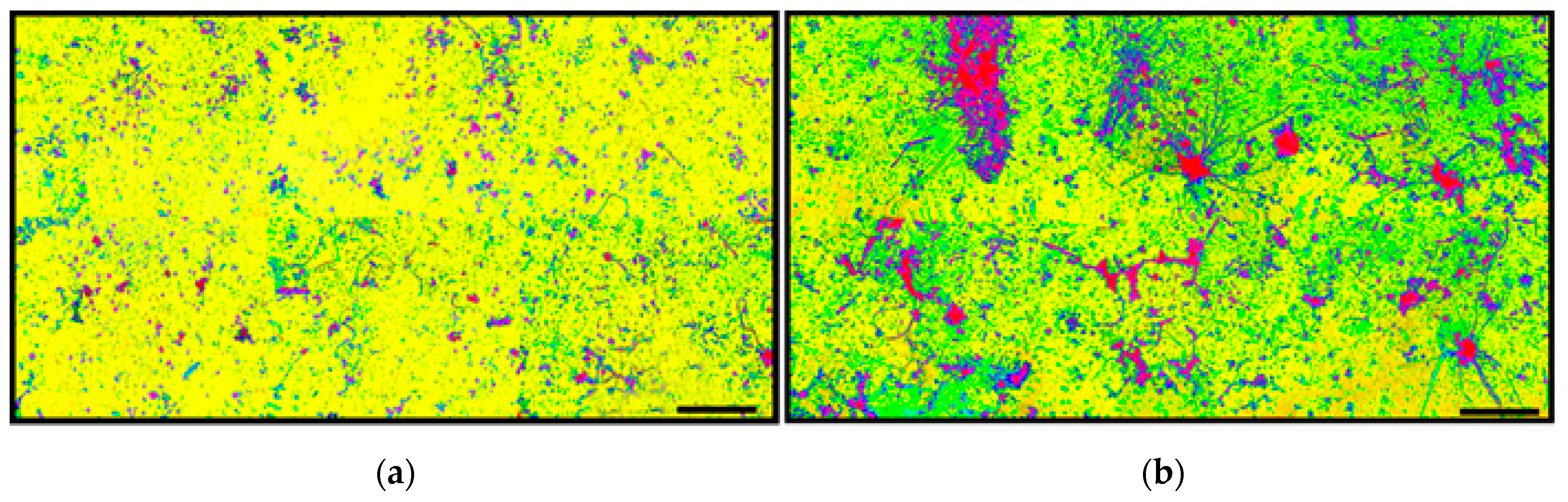
A second architectural analysis of microcolony biofilms was implemented to assess their surface texture. Figure 4a,b shows examples of heterogeneity in surface texture for biofilm communities A and B based on the varied distributions of their size and luminosity in pseudocolor rendered images prepared using the CMEIAS Color Segmentation tool [14]. 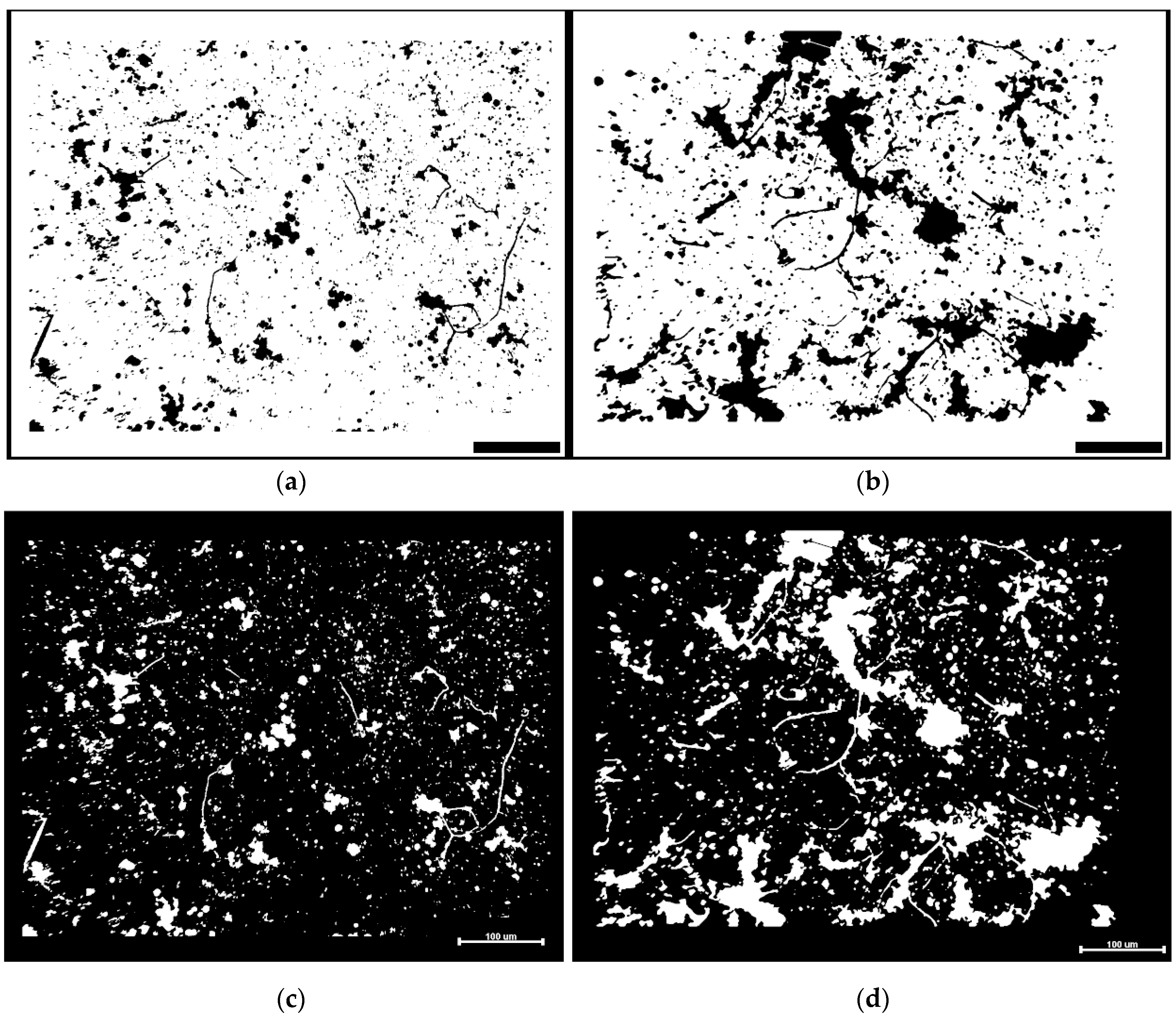This result indicates a greater variation and intensity of surface texture for the biofilm community B developed on the polystyrene substratum (Figure 4b). This brief test was followed by a grayscale brightness-based assessment of luminosity within images acquired using brightfield microscopy with transmitted light. In this case, microcolony biofilms display local heterogeneity in brightness intensity (on a scale of 0–255) due to variations in their height (third “z” dimension) inversely proportional to the amount of transmitted light that has scattered (hence been subtracted) as it passes through them during microscopic examination and image acquisition. Analysis of inverted grayscale images (e.g., Figure 1e,f) then directly relates microcolony height to luminosity brightness.

Biofilm surface texture was analyzed in situ using the integrated density metric that combines both the size and luminosity of the individual microcolonies (computed as the product of the object’s pixel area times its mean gray level). For quantitative analysis of surface texture, the integrated densities of community A and B biofilms were compared in eighteen 8-bit inverted grayscale images following a brightness threshold of 85% to find and segment their individual microcolony biofilms. A pair-wise dissimilarity analysis indicated significant differences in their overall distributions, with distance coefficients of 12.18% proportional dissimilarity, average Euclidian distance of 23.02, and Canberra distance of 0.64. The mean values of cumulative integrated density per image were 41,597 and 84,003 for communities A and B, respectively. Two-tailed statistical tests rejected the Ho of no difference between sample means (p = 1.84 × 10⁻³⁶), sample medians (p = 0.000) and variances (p = 0.000) of their integrated density, indicating that the surface texture of biofilm community B was more intensely heterogeneous with significantly more abundant, taller microcolony “mounds” in its three-dimensional (x, y, z) architecture on the polystyrene substratum, as further evidence of its greater productivity in this environment.

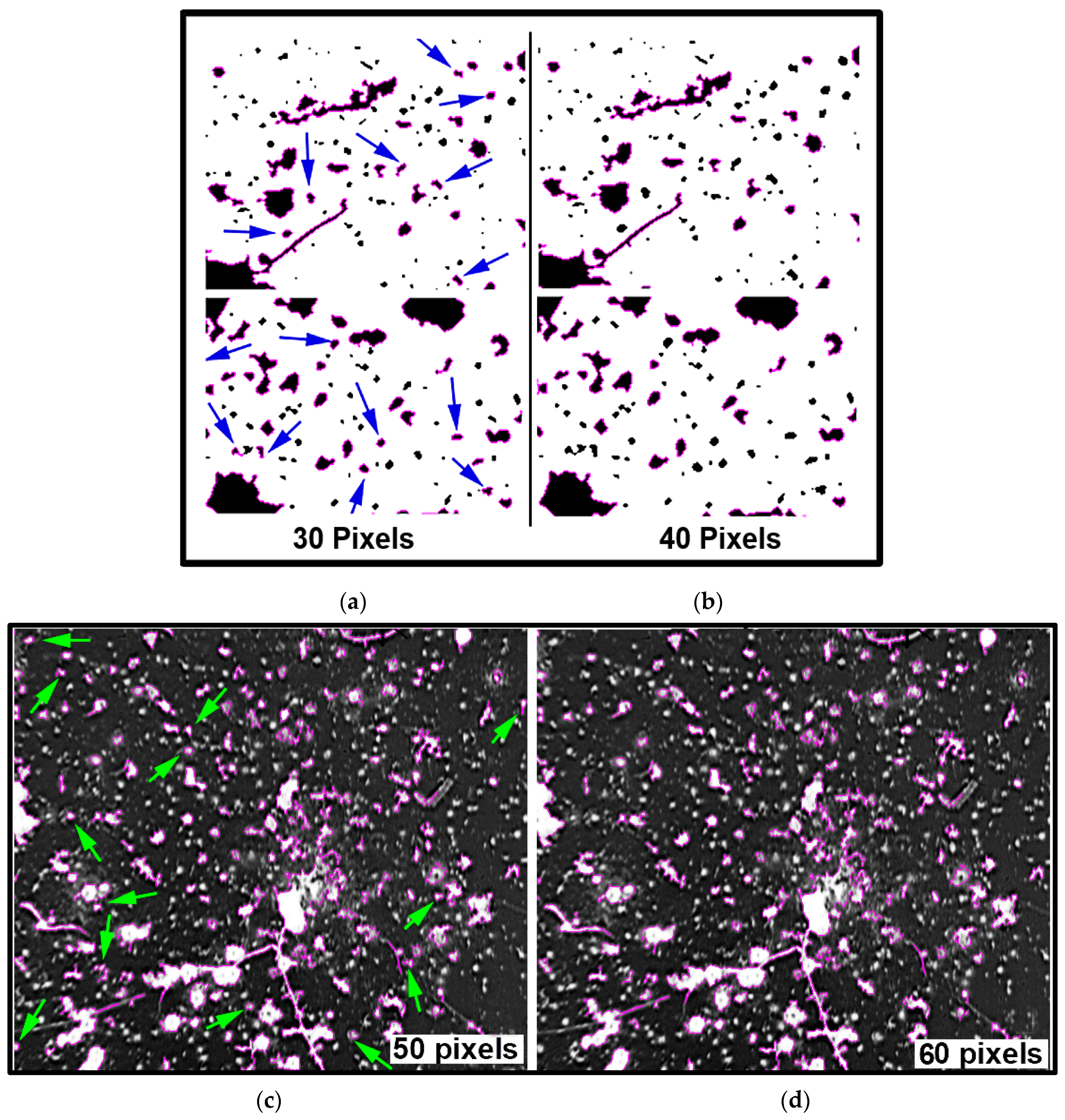
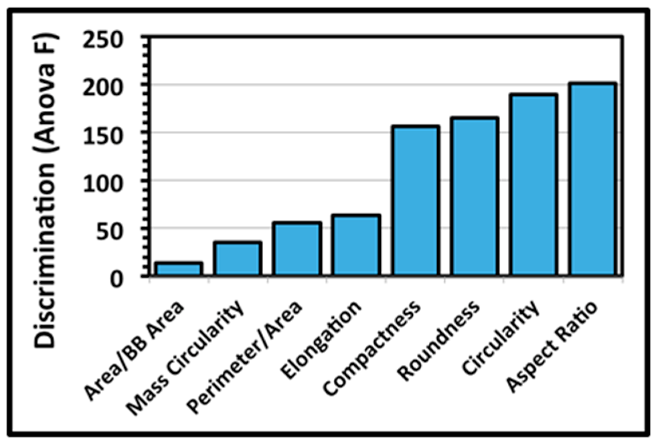
A third architectural analysis of the two communities of microcolony biofilms was implemented to assess differences in their two-dimensional shapes. The microcolonies >40 pixels in size within low-resolution binary images (25 per community) were analyzed by several metrics that evaluate the intensity at which their patch contour shapes deviate from a perfect circle of concentric radial growth. An ANOVA analysis indicated that the metrics of aspect ratio, circularity, roundness and compactness ranked highest in their ability to discriminate the microcolony shapes (Figure 5).

The extent of differences in contour shapes of microcolony biofilms of communities A and B was then tested using these four top-ranked discriminating metrics. A two-tailed multivariate statistical T-test indicated that the values of this shape feature for the two communities were not derived from the same distribution (ANOVA F 60.933, p (Ho of no difference) of 8.34 × 10⁻⁵¹). A two-tailed Student t-test of these four discriminating shape metrics analyzed separately indicated that the community A microcolonies on the plain glass substratum were significantly rounder and more compact (

Table 4. Statistical analysis of differences in architecture of microcolony biofilms developed on: plain glass (A); and polystyrene (B) substrata, based on four discriminating metrics of their contour shape.

Object Shape Metric	Community A	Community B	Two-Tailed t value	(p) Probability
Aspect Ratio	0.240 1	0.198	14.006	5.40 × 10−44
Circularity	0.485 1	0.404	13.603	1.24 × 10−37
Roundness	0.686 1	0.614	12.840	2.22 × 10−37
Compactness	0.761 1	0.721	12.516	1.29 × 10−35

¹ Significantly greater value at the indicated p level.

), concurring with a visual inspection of their reduced intensity of radial dispersion (Figure 1a,c and e).

3.3. Landscape Ecology of River Microbial Biofilms at Microcolony Spatial Resolution

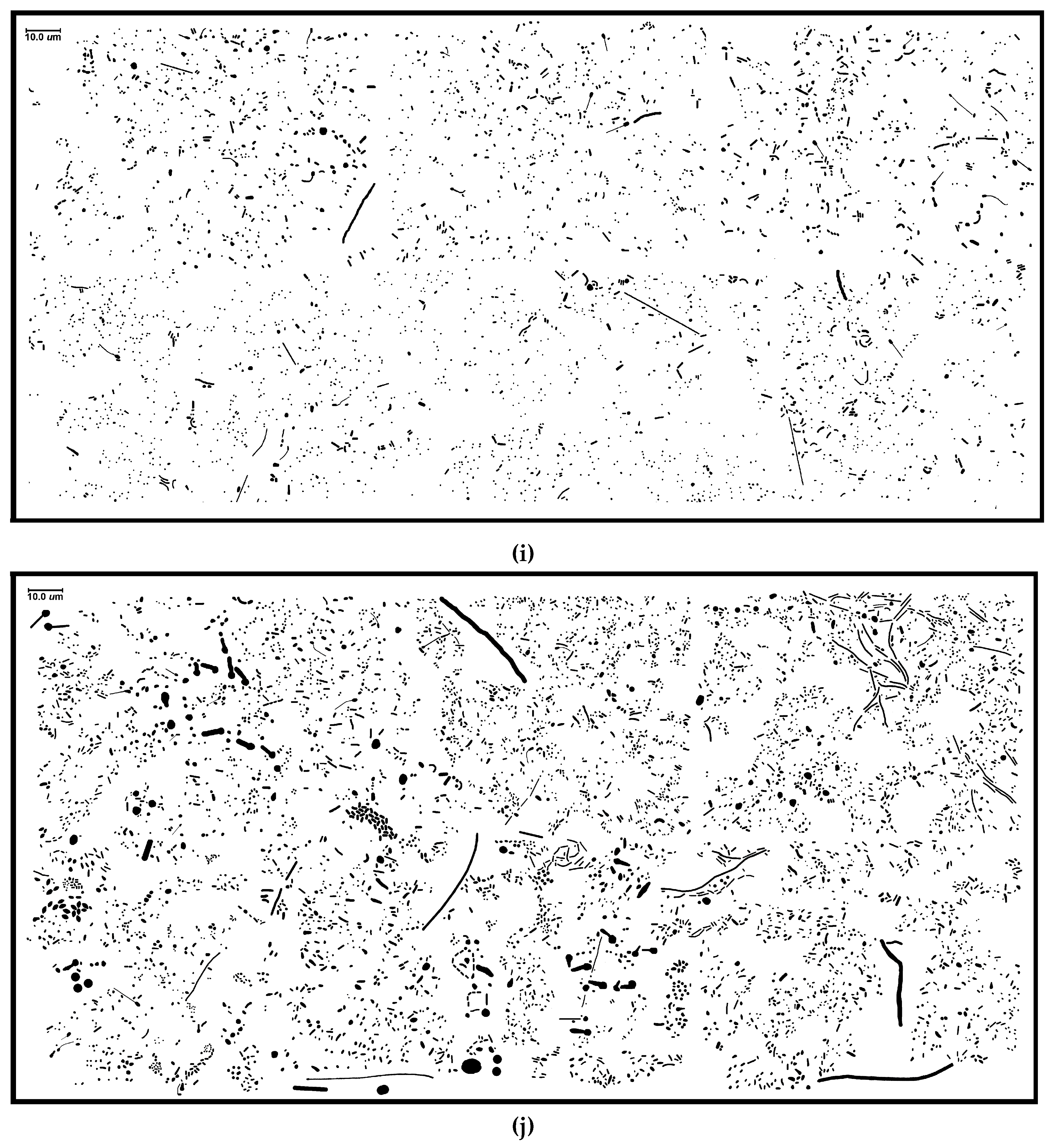
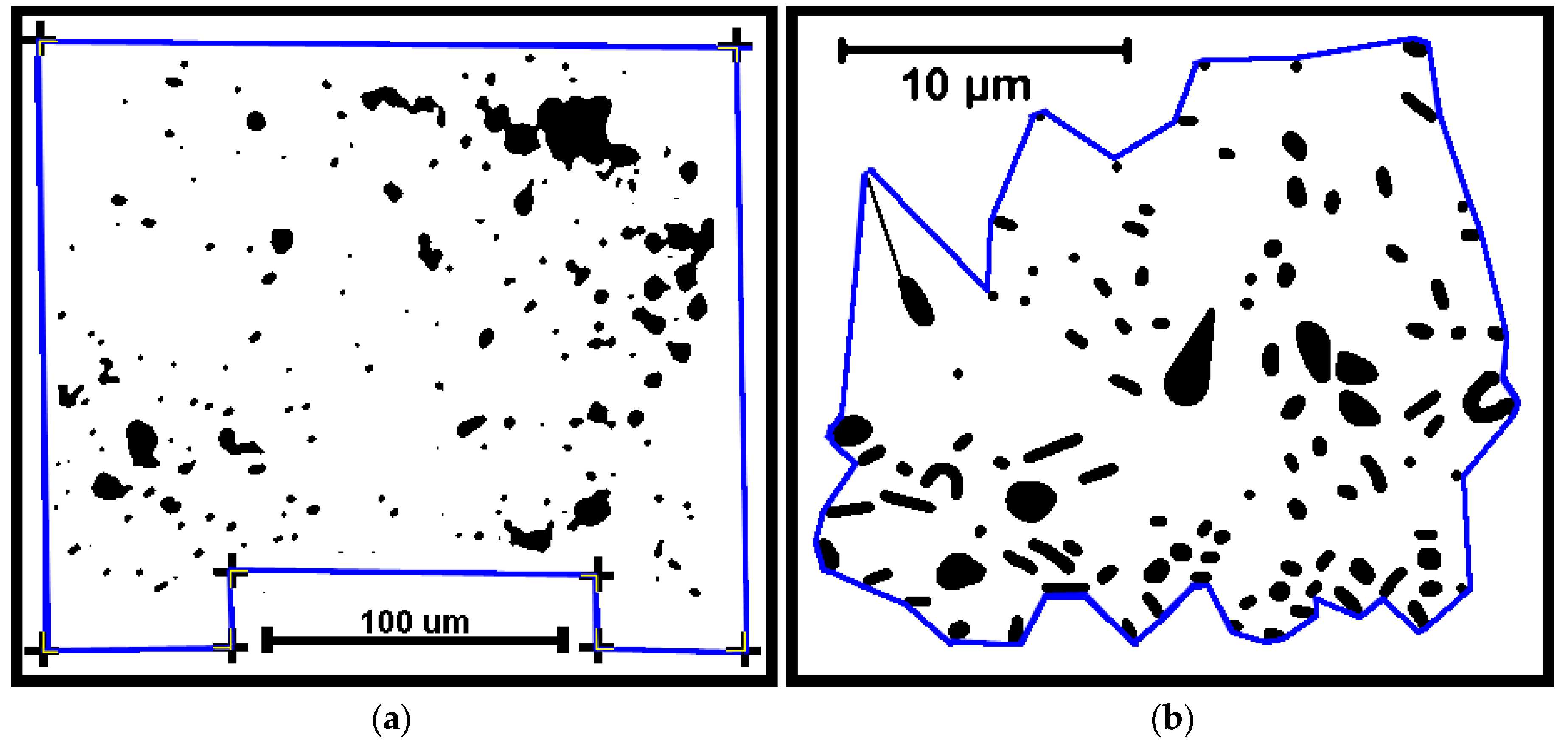
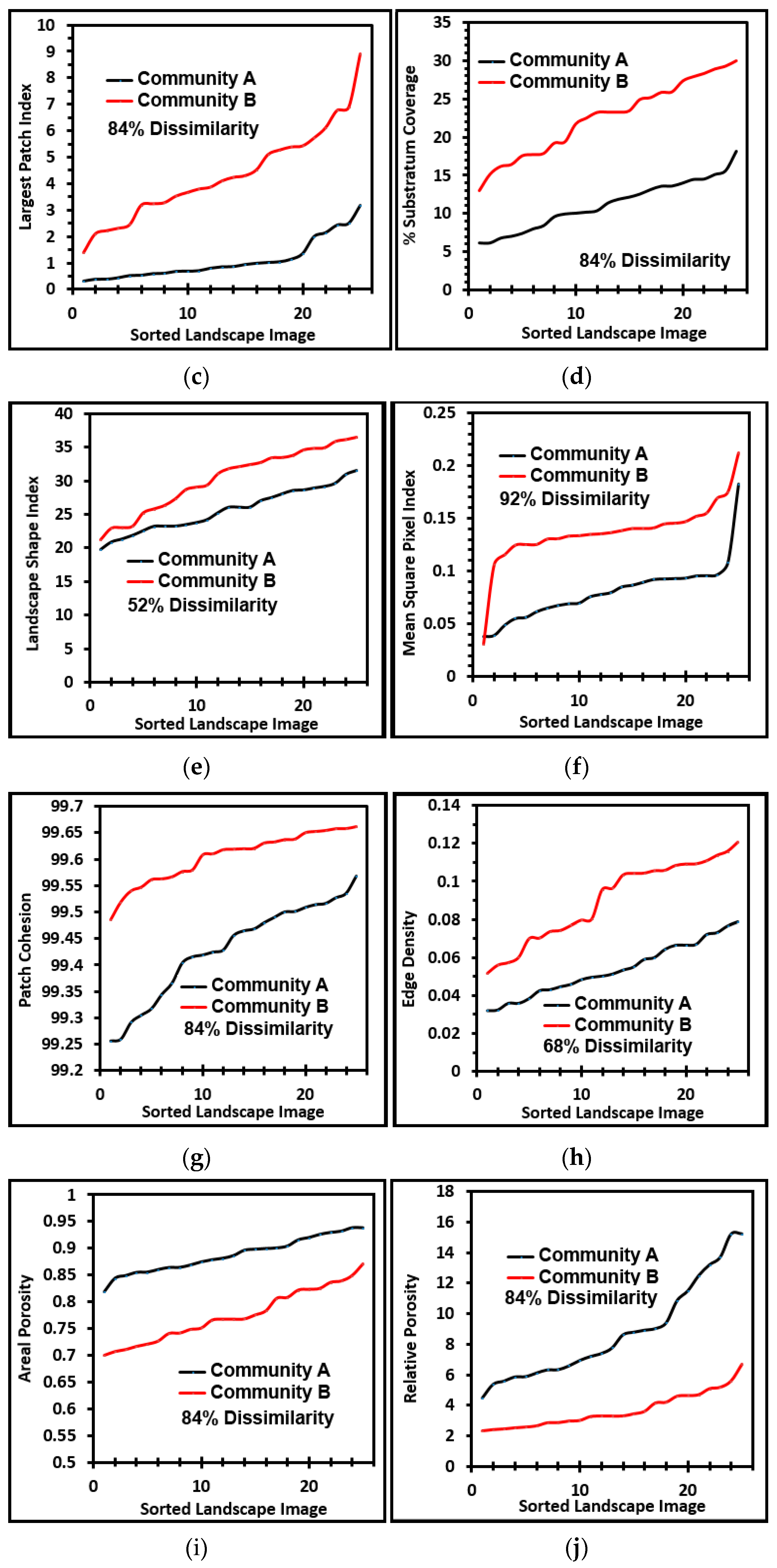
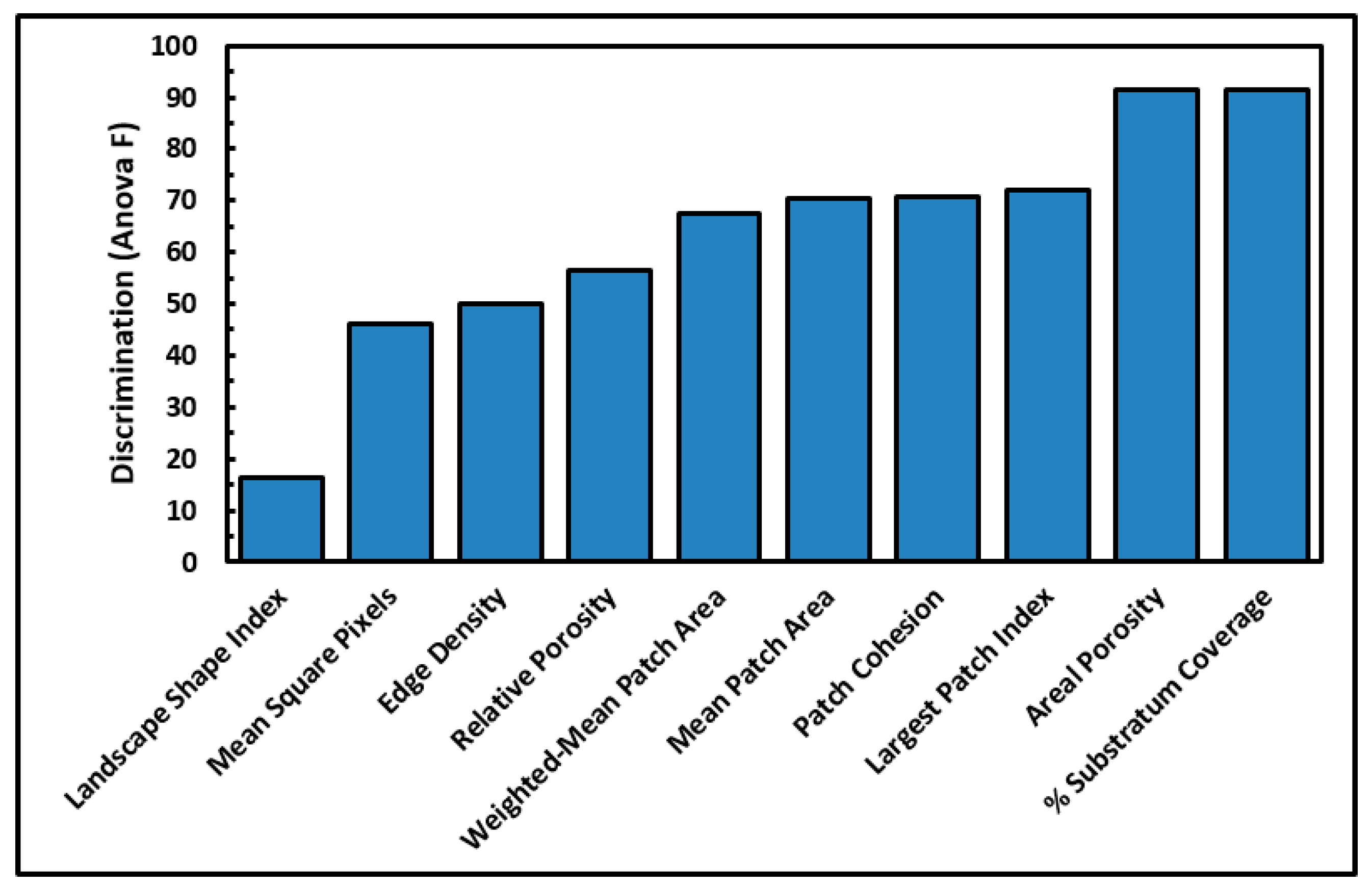
Several cumulative object analyses were done to characterize the mosaic of microcolony patches in the biofilm landscapes. They included categories of landscape ecology metrics that assess their patch area statistics (mean patch area, weighted-mean patch area, largest patch index), abundance and intensity of aggregated patches (percent substratum coverage), patch shape complexity (landscape shape index, mean square pixels), patch aggregation/dispersion/interspersion/fragmentation/connectivity (patch cohesion), patch edge intensity (edge density), and landscape porosity of fluid-filled channels between microcolony biofilm patches (areal porosity, relative porosity). Each metric was used to analyze microcolony biofilms >40 pixels in size in low-resolution binary images (25 per community), using the cross-hair method to define the area of interest polygon when that information was needed to compute metric intensities weighted by the substratum area (Figure 2a).

The ranked ability of these landscape ecology metrics to discriminate biofilm architectures is shown in Figure 6, revealing that percent substratum coverage and areal porosity had the greatest discriminating power among this group. The mean values for all 10 landscape ecology metrics extracted from images of the two biofilm communities were tested by the two-tailed Student t-test, and their differences were all statistically very significant (p << 0.01) (

Table 5. Two-Tailed two-sample statistical t tests of significant differences between mean values of ranked landscape ecology metrics that distinguish the architecture of river microcolony biofilm communities developed on: plain glass (A); and polystyrene (B) substrata.

Landscape Ecology Index	Community A	Community B	Two-Tailed t Value	(p)
Landscape Shape Index	25.604	30.233 1	4.033	2.21 × 10−4
Mean Square Pixels	0.081	0.137 1	6.793	1.53 × 10−8
Edge Density	0.054	0.090 1	7.082	1.11 × 10−8
Relative Porosity	8.762 1	3.673	7.525	2.17 × 10−8
Mean Patch Area	75.56	138.19 1	8.392	2.29 × 10−9
Weighted Mean Patch Area	799.95	4352.91 1	8.211	4.71 × 10−9
Patch Cohesion	99.431	99.604 1	8.407	4.15 × 10−10
Largest Patch Index	1.077	4.317 1	8.491	8.22 × 10−10
Areal Porosity	0.888 1	0.775	9.557	4.26 × 10−12
Percent Substratum Coverage	11.23	22.52 1	9.65	4.23 × 10−12

¹ Significantly higher mean value based on the two-tailed test statistic for the 25 images of each biofilm.

).

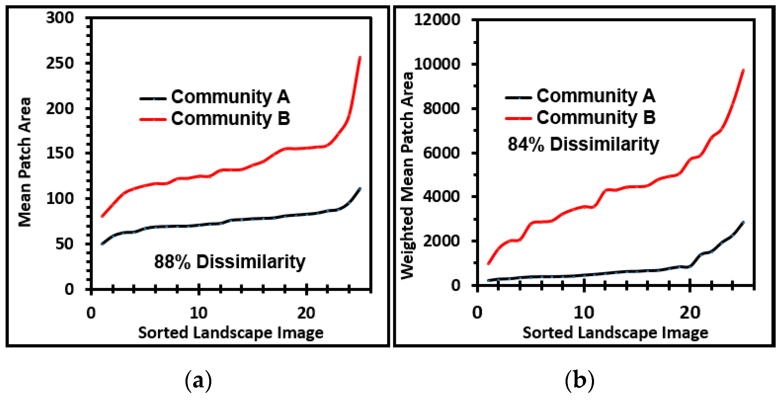
These metrics of landscape ecology were evaluated further by comparing paired ascending sort plots of their values extracted from images of the two biofilm communities. This analysis revealed clear separations in the distribution of ranked values for each metric of landscape ecology examined (Figure 7a–j), confirming that all were able to discriminate the biofilm architectures of these two communities developed on contrasting substrata. Consistent with the visual evidence provided by representative biofilm images (Figure 1a–f), these data further corroborate that the microcolony biofilms of community B developed a more dense and discrete landscape pattern, interpreted as having more productivity (more aggregated patches and larger sizes covering a significantly larger portion of the substratum area, hence less void spaces), greater edge intensities and complex shapes enabling their greater exploitation of external resources, significantly enhanced connectivity between neighboring microcolony patches (often via thin filamentous interconnections; see Figure 1b,f) that would potentially extend their “calling distances” in cell–cell communication, and more access to additional opportunities for syntrophic-like cross-feeding and other positive interactions with community members, ultimately resulting in further growth expansion on the polystyrene substratum [5,18,24,29,38,53,54,55,56,61,62].

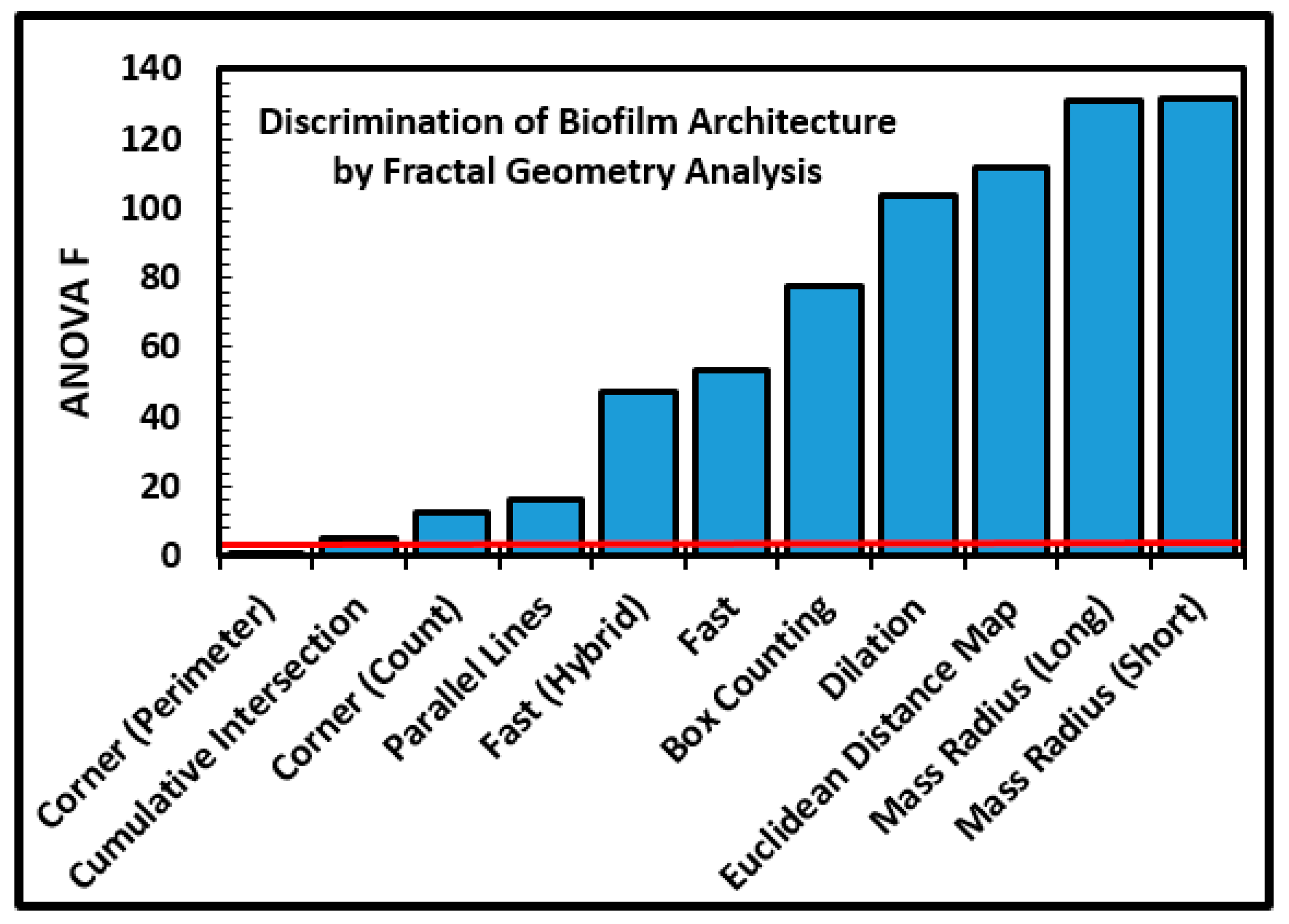
These architectural differences between the two communities of microcolony biofilms prompted us to explore the fractal geometry component of their landscape architecture. We anticipated that the more productive microstructured biofilm of community B would exhibit a greater fractal dimension on the polystyrene substratum, reflecting its more intense colonization behavior of successful positioning to maximize nutrient resource acquisition and allocation within the hierarchical fractal-like nature of resource distribution networks within landscape microenvironments [5,7,15,25,26,27,30,31,32,34]. The fractal dimensions of microcolony biofilm coastlines in the inverted grayscale images were analyzed using optimized segmentation settings (Table 1), an 85% brightness threshold, and all 11 methods of fractal analysis using the automated batch process available in CMEIAS JFrad software [15]. A univariate ANOVA analysis of the data indicated that nine of the 11 methods had sufficient discriminating power to discern substantially different intensities of fractal geometry between the two biofilm communities (Figure 8). The variation in discriminating power is readily apparent among the 11 fractal methods in JFrad, illustrating the benefit of statistical data mining when the most discriminating methods of fractal analysis are not known beforehand.

A two-tailed two-sample multivariate Student t test indicated that the nine discriminating methods combined together found very significant differences in fractal geometry of the microcolony biofilms in the two communities (

Table 6. Two-tailed Student t statistical test of nine discriminating methods to compare the fractal geometry of river microcolony biofilm communities developed on: plain glass (A); and polystyrene (B) substrata.

Fractal Method	Community A	Community B	Student t Value	(p)	Community Interpretation
Corner Count	1.379	1.414	3.526	1.12 × 10−3	B >> A
Parallel Lines	1.369	1.387	3.998	2.84 × 10−4	B >> A
Fast (Hybrid)	1.296	1.319	6.867	3.73 × 10−8	B >> A
Fast	1.246	1.268	7.330	8.84 × 10−9	B >> A
Box Counting	1.371	1.614	8.807	1.08 × 10−9	B >> A
Dilation	1.411	1.573	10.190	2.97 × 10−11	B >> A
Euclidean Distance Map	1.372	1.540	10.553	1.29 × 10−11	B >> A
Mass Radius (Long)	1.327	1.469	11.435	1.85 × 10−12	B >> A
Mass Radius (Short)	1.328	1.471	11.475	1.69 × 10−12	B >> A
Two-sample multivariable two-sided t test	t2 = 198.22			2.27 × 10−8	B >> A

). In addition, the two-tailed two-sample statistical tests for each of these discriminating methods of fractal dimension analysis evaluated separately had very low p values that rejected the null hypothesis of no difference between the two communities (Table 6). The microcolony biofilm architecture was significantly more fractal when developed on the polystyrene substratum than on plain glass, predictably reflecting different fractal distributions of available growth-supporting resources and opportunities for species coexistence [25,26,27,31,32].

3.4. Morphological Analysis of River Microbial Biofilms Analyzed at Single-Cell Resolution

Morphological analysis provides a strong complement to genotypic and other phenotypic methods of polyphasic taxonomy to deliver important insights on microbial community structure and function. The list of morphotype-weighted examples is long, including community productivity, biodiversity, dominance, conditional rarity, niche apportionments, food-web dynamics, ecological succession/resilience and other membership-environment relationships when competing for limiting resources, adaptations to various environmental stresses (e.g., starvation, predation, eutrophication, etc.) and spatio-temporal dispersal activities [2,3,4,5,8,16,25,28,48,49,50,51,52,57,58,59,60,61,62,63]. The unique, supervised, hierarchical morphotype classifier featured in CMEIAS uses mathematical rules of pattern recognition algorithms operating in 14-dimensional feature space to classify all major and several minor microbial morphotypes of individual cells, and performs with an overall 96% accuracy on properly edited images [2,13]. 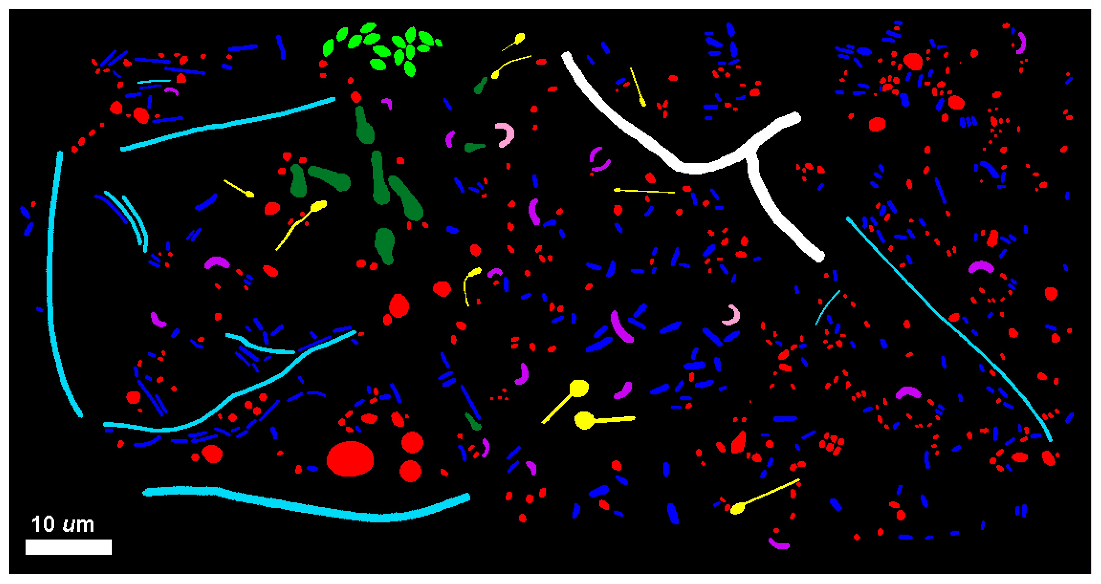This classifier also automatically produces a rendered image containing each cell differentially pseudocolored in situ to indicate its assigned morphotype class [2]. This latter software feature was used to produce the Figure 9 composite image illustrating the diversity of microbial morphotypes present in the river biofilm assemblages.

High-resolution images of individual microbial cells spatially distributed in situ within each biofilm community were combined into montages and analyzed. The distributions of cell abundance among the ranked morphotype classes are presented in

Table 7. Morphological classification of river biofilm community assemblages developed on: plain glass (A); and polystyrene (B) substrata and analyzed at single-cell resolution.

Morphotype Class	Ranked Class Abundance
	Community A	Community B
Coccus	10,660	15,377
Regular Rod	2935	5972
Curved Rod	121	84
Prosthecate	67	46
Unbranched Filament	48	86
Club	7	38
Ellipsoid	6	49
U-Shaped Rod	4	11
Branched Filament	1	1
Total Cells (24 images)	13,849	21,664

. This equivalent sampling effort indicated that the biofilm community B had a 56.2% greater cell abundance. Both community assemblages had an equal richness of the same nine morphotypes, a dominance of cocci (77% of community A and 71% of community B), and a rare singleton of one branched filament.

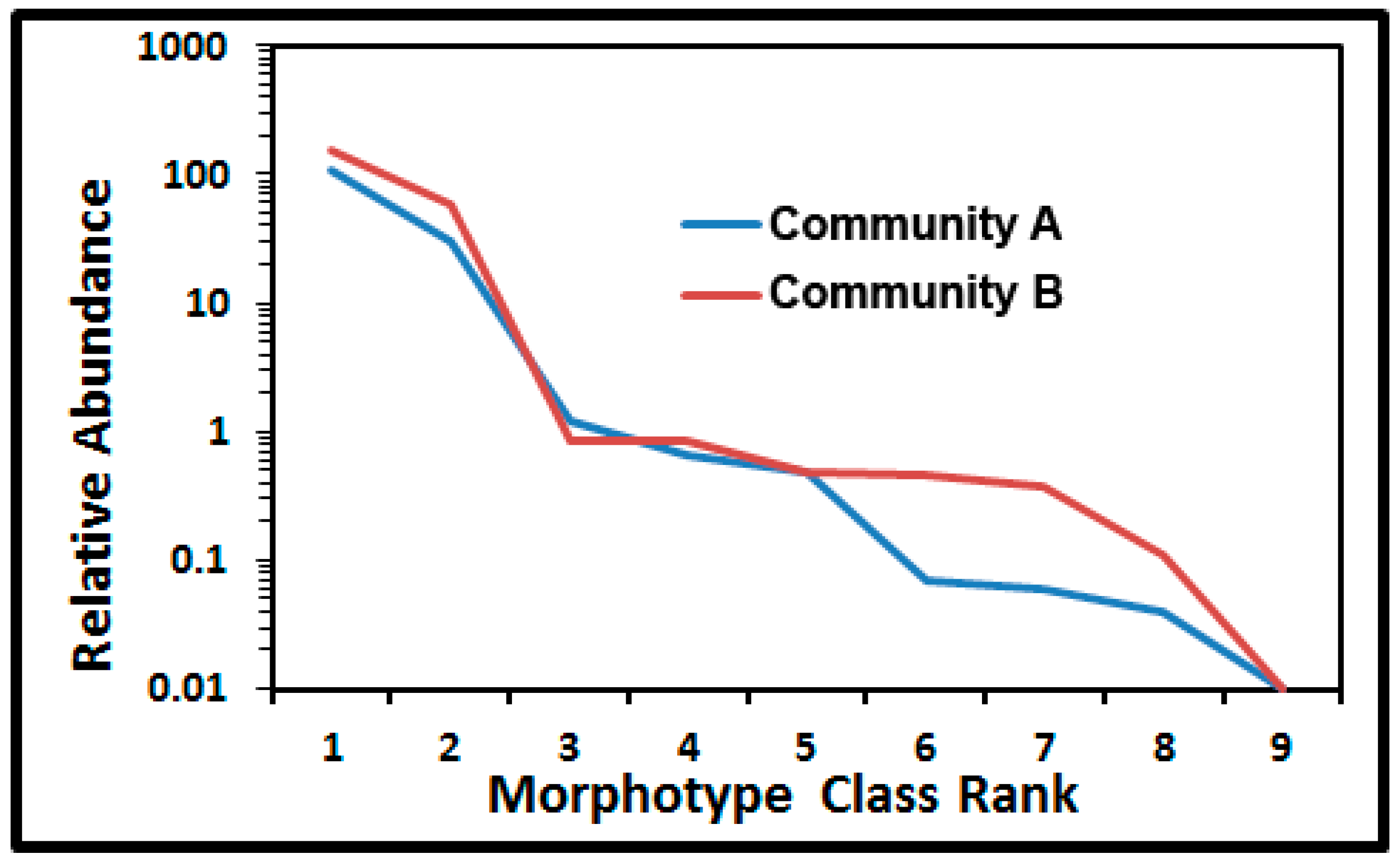
The diversity of these class distributions was examined by several methods of community analysis [5,28,42,43]. The shape of the Whittaker ranked abundance plot [28,43] showcases differences in relative numerical abundances, dominance and evenness of each morphotype class in communities A and B (Figure 10). The major separation of relative abundance in the curves occurred with rare morphotypes ranked as No. 6, 7, and 8 (clubs, ellipsoids and U-shaped rods). The abundance in these numerical ranked distributions was greater for six of the nine morphotypes colonizing the polystyrene surface. Based on the least difference between observed and expected values, the truncated logarithmic series model made the best fit to both curves because the abundance of intermediate classes was more common than predicted by the geometric model series, and their curves were steeper than the broken stick model or the sigmoid curve of the log normal model [28,43]. The singleton morphotype caused the slight truncation in the models for both communities.

Table 8. Indices of α-diversity, evenness, and dominance for comparison of morphological diversity in river microbial biofilm communities developed on: plain glass (A); and polystyrene (B) substrata.

Community Structure Indices	Community A (Raw)	Community B (Raw)	Community A (Normalized)	Community B (Normalized)
Shannon–Wiener Diversity	0.627	0.684 1	0.627	0.685 1
Simpson’s Diversity (1/D)	1.569	1.725 1	1.569	1.725 1
McIntosh Diversity	0.203	0.240 1	0.204	0.241 1
Brillouin Diversity	0.626	0.683 1	0.625	0.683 1
Q Statistic Diversity	1.332	4.897 1	1.299	5.009 1
McIntosh Evenness	0.302	0.358 1	0.302	0.358 1
Brillouin Evenness	0.285	0.311 1	0.285	0.312 1
Camargo Evenness	0.402	0.489 1	0.402	0.489 1
Smith and Wilson Evenness (1-D)	0.408	0.473 1	0.408	0.473 1
Berger-Parker Dominance	0.770 1	0.710	0.770 1	0.710

¹ Community with the statistically significant (p ≤ 0.05) higher index value based on the Solow test. D: Simpson’s Dominance Index.

indicates various indices of community α-diversity, evenness and dominance computed from the data of raw numerical abundance (individual counts) (Table 7), and after a relative normalized transformation (% ×100) of those same data to equalize community sample sizes. Data normalization only marginally affected the computed indices (likely because both communities had an equal richness of the same nine morphotype classes) without affect their ranking. The robust 10,000-iterated Solow statistic test [43,64] indicated that the diversity and evenness indices were significantly higher (p ≤ 0.05) for the river biofilm community B on the polystyrene substratum. Correspondingly, the dominance index was significantly higher for the community A developed on plain glass. These results agree with other studies indicating that community diversity strongly correlates with larger sizes and complex structures of landscape patches [24].

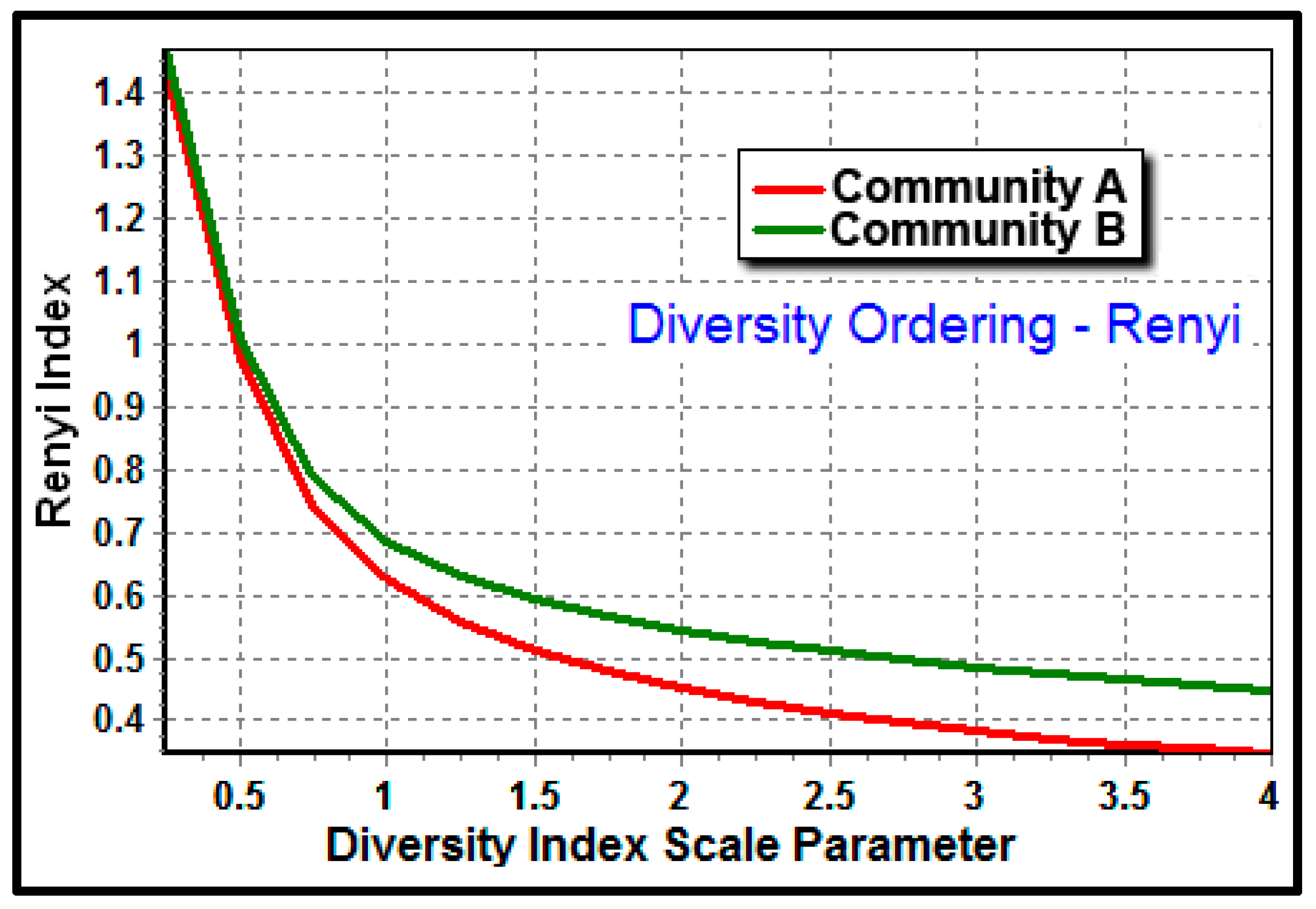
The Renyi ordering analysis provides a robust, entropy-based test of whether the trends of α-diversity that differ between communities change with the diversity index used, and allows the relative magnitude of α-diversity across a range of indices to be compared directly [43,65]. This analysis of the ranked abundance of morphotype classes for the two communities (Figure 11) showed that their ranges of diversity indices do not cross one another indicating that they are validly comparable, and that community B developed on the polystyrene substratum had a higher Renyi index at each point of the scaled indices, validating its greater morphological diversity.

β-Diversity indications of the degree of differences in distribution of ranked abundance among morphotype classes of communities A and B are provided in computations of various dissimilarity (distance) coefficients (

Table 9. β-Diversity coefficients of dissimilarity (distance) between morphotype class distributions in river biofilm communities developed on plain glass and polystyrene substrata.

Distance (Dissimilarity) Coefficients	Value
Percent Proportional Dissimilarity	6.754
Euclidian Distance	5610.120
Average Euclidian Distance	1870.222
Canberra Distance	0.346
Bray–Curtis Distance	0.223
Chord Distance	0.102
Geodesic Distance	0.455
Manhattan Distance	7754
Mahalanobis Distance	2.529
Renkonen Distance	0.936

) [42] and in plots that examine the communal relationships of their ranked dominance and rarity (Figure 12a,b) [5,25,28,66,67].

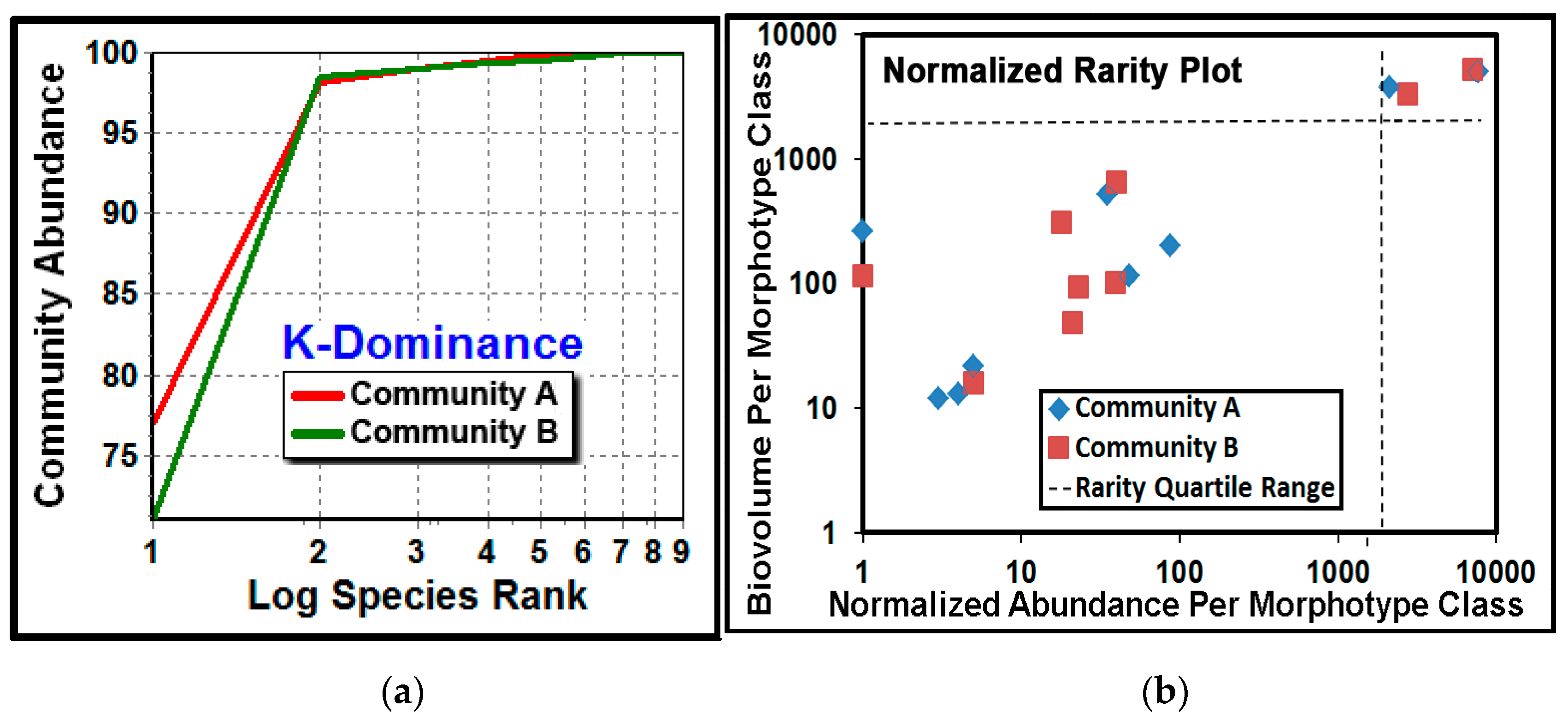
The K-dominance analysis compares the cumulative abundance of classes as a percentage against their log class rank in the community [5,28,43,66]. The result showed that community A had a higher dominance of its most abundant cocci morphotype (Figure 12a). The normalized rarity plot [5,28,67] compares the relative abundance and cumulative biovolume for each morphotype class in the community, and identifies community classes that are considered “rare” when they locate within the lower left quadrant (25th percentile) of the plot range. This analysis indicated that most of the class richness was represented by the seven rare morphotypes (comprising ≤25% of the class abundances), and the relative abundances of their cumulative biomass were similar for some morphotype classes but different for others (Figure 12b). This latter result also suggests that rarity for some morphotype classes may be “conditional” because their relative abundances were affected by the substratum environment upon which they had colonized [68]. This finding has potential importance because conditionally rare classes can contribute significantly to community stability and resilience during the ecological succession that follows environmental perturbation [2,3,4].

3.5. In Situ Ecophysiology of River Microbial Biofilm Communities Analyzed at Single-Cell Resolution

CMEIAS bioimage informatics were used to analyze traits of community ecophysiology in situ, including their intensity and productivity of biofilm colonization, allometric metabolic rate, and indicators of adaptations to starvation and predatory stresses [5,10,13,33,34,35,36,37,48,49,50,51,52,57,58,59,60]. The strengths of these vital activities were compared in images of the two river biofilm communities using data of each cell’s biovolume, surface area/biovolume ratio, and relative lengths of elongated cells.

Table 10. Productive colonization intensity, biovolume, biomass carbon and active allometric metabolic rates (AMR) in river biofilm communities developed on: plain glass (A); and polystyrene (B) substrata and analyzed at single-cell resolution.

Measurement Type (Units)	Community A	Community B
Total cell count (all images)	13,849	21,664
Spatial Density (cells/mm2)	108,909	199,862
Percent Microbial Coverage of the Analyzed Substratum	5.11	8.67
Total Cell Biovolume (μm3; all images)	3,197.748	5593.425
Cell Biovolume Intensity (μm3/mm2 substratum)	25,367.4	51,586.5
Mean Cell Biovolume (μm3/cell)	0.233	0.258
Median Cell Biovolume (μm3/cell)	0.079	0.136
Cell Biomass Carbon Intensity (pg C/mm2 substratum)	1809.4	3568.6
Cumulative Active AMR (nanoWatts; all images)	354.401	1060.348
Active AMR Intensity (picoWatts/mm2 substratum)	2811.43	9783.83
Active AMR per cell (femtoWatts)	25.590	48.932

presents data on the substratum area-weighted intensity of productive colonization and cell size-weighted allometric metabolic rates with equal sampling efforts for both communities. The total cell counts, spatial density, substratum coverage and cumulative biovolume intensities were 1.56–2.03-fold higher for community B. This greater intensity of biomass is consistent with earlier results (Table 2 and Table 3) indicating a larger, more abundant/widespread/highly structured architecture of microcolony biofilms for the corresponding community. Two-sample two-tailed statistical tests indicated that the differences between means were highly significant for spatial density (p = 0.0001), and significant for biovolume intensity (p = 0.02), mean cell biovolume (p = 0.04) and median cell biovolume (p = 3.81 × 10⁻⁴⁷). Thus, individual microbial cells were significantly bigger and more abundant when colonized on the polystyrene substratum. Since the metrics of biomass carbon and active allometric metabolic rates are derived from cell biovolume [33,34,35,36,37,46,47,48,49], they had the same trend of significantly higher substratum area-weighted intensities and metabolic rate per individual cell in community B. Considered collectively, these results provide evidence to indicate that biofilm community B was more metabolically active and better able to convert resources into biomass resulting in its greater overall productivity on the polystyrene substratum in the river ecosystem.

The relative abundance of populations within a community assemblage to some extent reflects their success at competing for limited resources [5,28], and therefore the metric used to measure abundance in community membership can significantly influence how variations in that relationship are interpreted. This issue applies to all metrics used to measure class abundances in community analysis [5]. Use of the CMEIAS morphotype classifier made it possible to examine the distribution of cell biovolumes and their size-scaled allometric metabolic rates among individual morphotype classes (singleton excluded). This analysis indicated a higher productivity for the biofilm community B (Table 10,

Table 11. Distribution of individual cell biovolumes among morphotype classes in river biofilm communities developed on: plain glass (A); and polystyrene (B) substrata.

Morphotype Class	Community A 1	Community B 1	Community A Intensity 2	Community B Intensity 2
Coccus	50.978	52.917	12,919.040	24,365.564
Curved Rod	2.027	1.018	513.600	468.836
U-shaped Rod	0.117	0.160	29.633	73.796
Regular Rod	37.596	33.450	9527.573	15,402.069
Unbranched Filament	4.364	6.494	1105.834	2989.937
Ellipsoid	0.126	0.935	32.040	430.328
Club	0.222	3.080	56.290	1418.034
Prosthecate	1.944	0.777	492.565	357.892

¹ Percent of total community biovolume. ² Unit of intensity is μm³/mm² of substratum area.

and

Table 12. Distribution of active allometric metabolic rates among morphotype classes in river biofilm communities developed on: plain glass (A); and polystyrene (B) substrata.

Morphotype Class	Community A Metabolic Rate (picoWatts)	Community B Metabolic Rate (picoWatts)	Community A Intensity of Metabolic Rate (picoWatts/mm2)	Community B Intensity of Metabolic Rate (picoWatts/mm2)
Coccus	13.070	29.302	102.782	240.557
Curved Rod	1.731	1.889	13.610	15.505
U-shaped Rod	0.170	0.355	1.340	2.912
Regular Rod	24.810	29.556	195.108	242.638
Unbranched Filament	18.902	69.734	148.647	572.489
Ellipsoid	0.155	2.732	1.058	22.431
Club	0.350	35.398	2.755	290.604
Prosthecate	2.812	1.904	22.116	15.630

). Over 90% of the total biovolume was distributed among the cocci, unbranched filament, and regular rod morphotaxa classes. The difference between means for the biovolume intensity was statistically significant (p < 0.05) for the cocci and marginally significant (p = 0.054) for the regular rods. Although the cumulative biovolume and biovolume intensity were also greater for the U-shape rod, unbranched filament, ellipsoid and club morphotypes in community B (Table 11), the range of their individual cell size was substantial, resulting in mean differences that were not statistically significant. The cocci, curved rods, U-shaped rods, regular rods, unbranched filaments, ellipsoids and clubs each had higher cumulative metabolic rates and metabolic rate intensities in community B (Table 12).

Further morphotype-weighted analyses of biofilm communities at single-cell resolution provided additional insights on their productivity and adaptive responses to environmental stresses. For instance, sizing down to increase the cell’s surface area/biovolume ratio is one of several self-induced responses used particularly by K strategists to adapt to starvation stress, and this morphological change is often accompanied by: (i) expression of transport systems with higher affinity and others with broader specificity that improve their ability to acquire essential nutrients when their local apportionment is low; (ii) enhanced distribution of those resources within the cell; and (iii) turnover of excess ribosomes and internal reserves of storage polymers [5,50,51,52]. An analysis of all cells in the two communities indicated that their surface area/biovolume ratios had dissimilar distributions (40.32% proportional dissimilarity, 495.65 average Eucledian distance, 0.515 Bray–Curtis distance, and 0.651 Canberra distance). Most of this pair-wise dissimilarity was attributed to the coccus morphotype, which differed between the two communities by distance coefficients of 51.34% proportional dissimilarity, 540.56 average Eucledian distance, 0.589 Bray–Curtis distance, and 0.662 Canberra distance. The mean and median values of the surface area/volume ratio were significantly higher for all cells and for the coccus morphotype in community A developed on the plain glass substratum, and the probability (p) that these values differed by chance was extremely low (

Table 13. Comparison of surface area/biovolume ratios for cells in river biofilm communities A and B developed on plain glass and polystyrene substrata, respectively.

Cells Sampled (N)	Mean (p for Student t)	Median (p for Mann–Whitney)
Community A all sampled cells (13,849)	11.835 (1.09 × 10−73)	12.281 (0.000)
Community B all sampled cells (21,664)	11.124	10.507
Community A cocci only (10,660)	12.686 (4.31 × 10−92)	14.762 (0.000)
Community B cocci only (15,377)	11.774	11.086

).

Bacteriovory grazing activities by heterotrophic protozoan nanoflagellates and metazoan predators are important forces that shape the structure and composition of bacterial communities in aquatic ecosystems, largely because resistance to and refuge from selective bacteriovory are favored by large cell aggregates (e.g., microcolony biofilms) and elongated filamentous morphologies (e.g., unbranched filament) that exceed the oral diameter of the cytosome or lorica mouth opening of the predator, thereby increasing the predator’s difficulty to consume the microbial prey [5,48,57,58,59,60,63]. Thus, bacteriovory predation is both size-selective and morphology-selective, and the relative abundance and length of the unbranched filament morphotype can provide insights on the intensity of the selective pressure of phagotrophic predatory stress that contributes to shaping the aquatic microbial community, in line with the evolutionary pressures to maximize resource intake [5,25]. That indicator morphotype had a 79.2% greater abundance (Table 7), 21.1% greater cumulative length and 26.4% greater length intensity in the biofilm community B (

Table 14. Cell length analysis of the elongated unbranched filament morphotype in equal sampling efforts of river biofilm communities A and B developed on plain glass and polystyrene substrata, respectively.

Cell Length Metric	Community A	Community B
Cumulative Length (μm)	926.6	1122.0
Length Intensity (μm/mm2)	7287.0	9211.3

). The two-sample two-tailed Student t tests indicated that these differences in communities A and B were statistically significant (p = 0.04). These results plus the larger sizes of microcolony biofilms indicated earlier (Table 2 and Table 3) predict that bacteriovory grazing activities and adaptations to resist them were more intense in the biofilm assemblage of community B, and the increased fitness of the larger microcolonies and longer elongated unbranched filaments amidst the selective predatory stress likely contributed to their increased relative abundance and productivity in these river biofilms [5,57,58,59,60,61,63]. These data-supported predictions also help to explain how the presence of predator bacteriovory tends to increase individual bacterial biomass under ambient nutrient conditions in aquatic ecosystems [48].

3.6. Spatial Ecology of River Microbial Biofilm Communities Analyzed at Single-Cell Resolution

The dependence of spatially structured heterogeneity on ecosystem function provides the impetus to include analyses of spatial ecology in studies of microbial biofilm communities [5,6,7,9,11,12,15,25,27,30,31,32,38,45,62,69,70,71,72,73,74]. Analysis of the in situ spatial patterns of microbes within biofilms reveals statistically defendable data that support ecological theories of biogeography indicating that their colonization behavior involves a spatially explicit process rather than occurs independent of their location in this microenvironment [5,6,7,25,31,38,69,70,71,72,73,74]. Spatial dependence is considered positive when neighboring organisms aggregate due to cooperative interactions that promote their localized productive growth, and is considered negative when conflicting/inhibitory interactions result in their uniform, self-avoiding colonization behavior [5,6,7,9,27,30,38,61,69,70,71,72,73,74]. This balance between positive cooperation (aggregation) vs. conflicting competition (over-dispersion) behaviors is crucial in biofilm ecology [5,38]. For instance, microbial cells exert stronger intensities of quorum-sensing communication when closely aggregated within biofilms [9,62]. The analysis protocol to measure these distinctions of spatial patterns typically involves initial statistical tests of the null hypothesis of complete spatial randomness, followed by additional quantitative measures of spatial dispersion/aggregation, and finally by geostatistical analyses that test for the spatial autocorrelation, variation and connectivity in continuously distributed “z-variate” attributes of selected features (e.g., cluster index) at georeferenced X,Y coordinate locations of sampling points within the landscape domain [5,6,7,12,27,41,69,70,71,72,73,74].

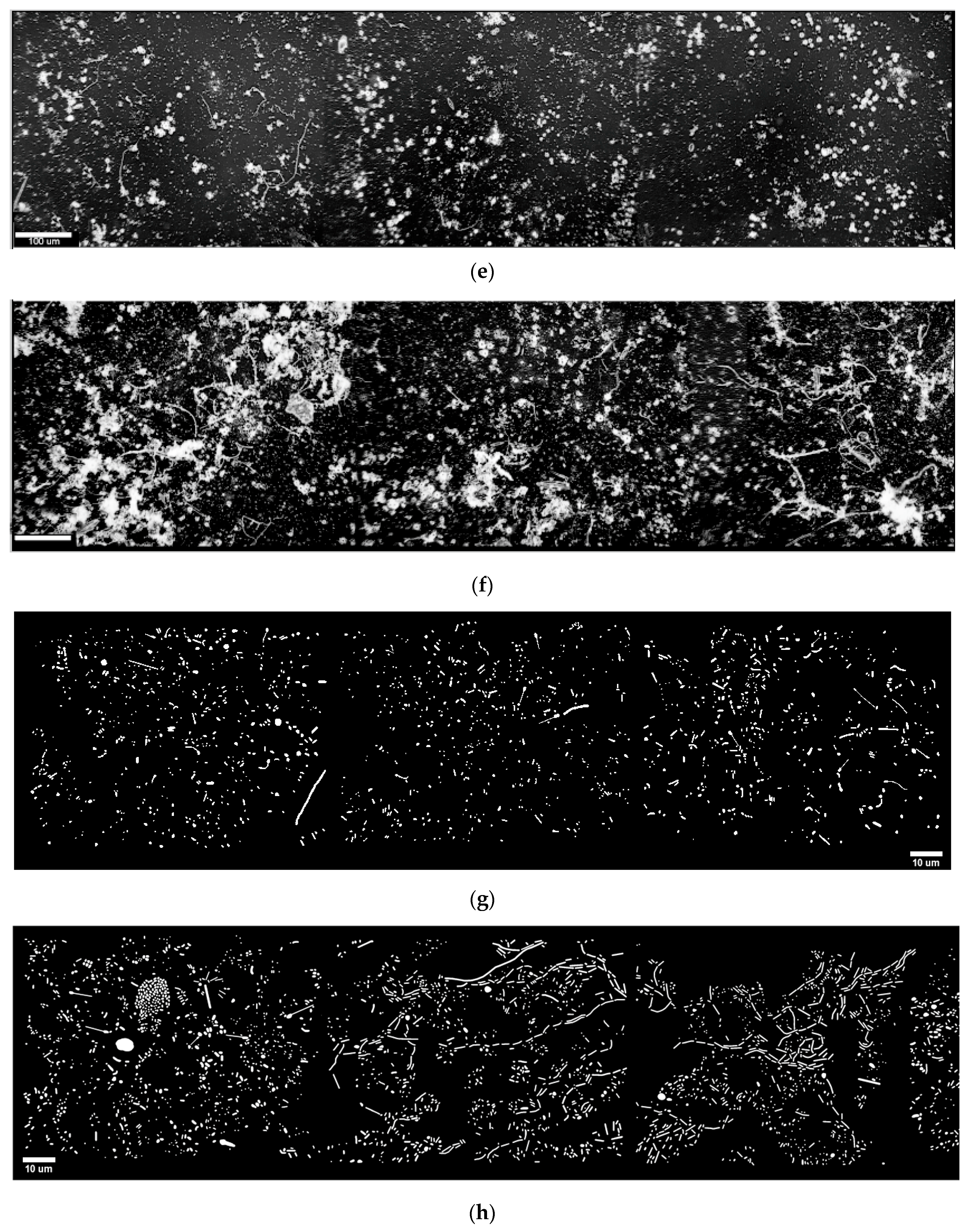
Several features were extracted from each individual cell for this spatial analysis [5,6,7,9,10,11,12,13,15,41,42,44,45,71,72], using optimized CMEIAS settings applied to high-resolution, fully segmented, spatially calibrated montage images of each community assemblage (Table 1; examples are Figure 1i,j). For instance, the proximity of neighboring cells impacts significantly on the intensity of successful cell–cell interactions in biofilms, e.g., in situ “calling distance” of quorum sensing-mediated communication [5,9,62]. Statistical analyses of the 1st nearest neighbor distance indicated that neighboring cells were positioned further apart in the river biofilm community A developed on plain glass, indicating a greater proximity of cells in community B developed on the polystyrene substratum (

Table 15. Comparison of 1st nearest neighbor distance distributions for individual cells in river biofilm communities A and B developed on plain glass and polystyrene substrata, respectively.

Metric and Statistic Test	Community A (μm)	Community B (μm)
Sample mean ± std. error	1.63 ± 0.01	1.30 ± 0.01
Sample median	1.45	1.19
75th Percentile	2.01	1.54
Maximum	6.29	5.79
Two-tailed Student t	33.95 (p same means): 1.89 × 10−209 A >> B
Mann–Whitney U	2.84 × 107 (p same median): 1.15 × 10−183 A >> B

).

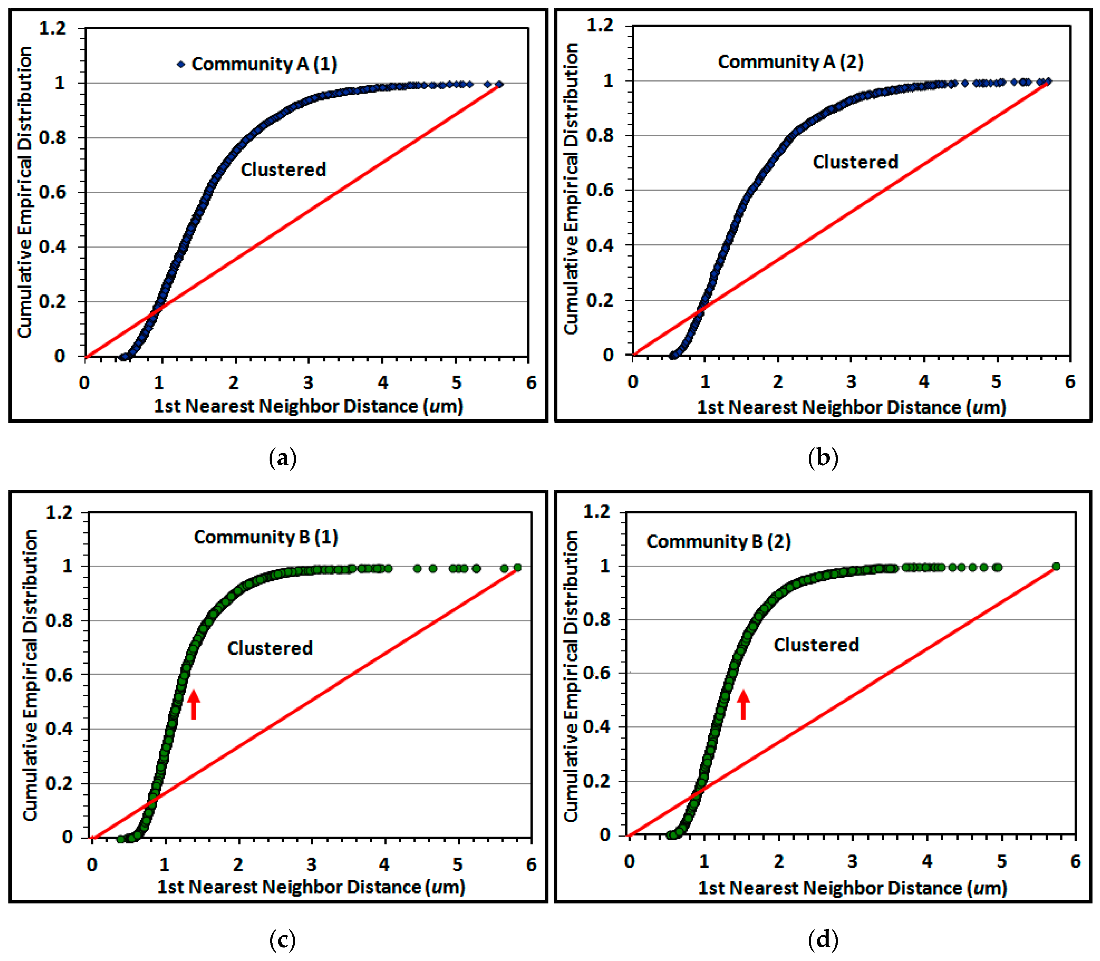
The Empirical Distribution Function (EDF) of 1st nearest neighbor distances between individual cells is a useful second test of spatial randomness. Its plot compares the cumulative rank of 1st nearest neighbor distances between individual cells in the biofilm community to the theoretical distribution that would occur if their pattern had complete spatial randomness [5,6,7]. Replicate empirical distribution plots for cells in the two river biofilms are shown in Figure 13a–d.

Random distributions in the EDF plot are defined by a diagonal line connecting the XY intercept to the maximum 1st nearest neighbor distance calculated by analysis. Data points on EDF plots of spatially structured communities are commonly characterized by a sigmoidal curve, with positions representing uniform spatial patterns when located below the theoretical random trendline, and aggregated (clustered) patterns when they rise above the diagonal trendline to the 1.00 EDF asymptote [5,6,7]. A random distribution is indicated if the EDF curve increases with a shallow slope close to the diagonal trendline. The results indicate that the proximity of cells in montage images of both communities has significant spatial structure, with a minority arranged in a uniformly equidistant spatial pattern and a significant majority that are spatially aggregated. Aggregated cells in community B on the polystyrene substratum display a steeper incline of their EDF curve (red arrows pointing upward) that reaches its asymptote at shorter (closer) distances between nearest neighbors (Figure 13c–d). These results show similarities in EDF of spatially aggregated cells in replicated montages of the same biofilm community (Figure 13a–d), and are consistent with visual inspection of local aggregate intensities within representative high-resolution images (Figure 1i,j).

The next tests of spatial point-patterns for these two biofilm communities evaluated the Holgate and Clark and Evans indices of cell aggregation based on each cell’s 1st and 2nd nearest neighbor distances and centroid X,Y coordinates, respectively [41,42,75,76]. These tests rejected the null hypothesis of complete spatial randomness for both communities (p < 0.05), and indicated significant aggregation in their overall spatial patterns of distribution (

Table 16. Point-pattern spatial aggregation analysis of cells in river biofilm communities. A and B developed on plain glass and polystyrene substrata, respectively.

Aggregation Test	Community A	Community B
Holgate A 1	0.544	0.591
Clark and Evans R 2	0.938	0.964

¹ Overall spatial pattern is significantly aggregated when A > 0.500. ² Overall spatial pattern is significantly aggregated when R < 1.000.

), consistent with the other spatial analyses of these two communities.

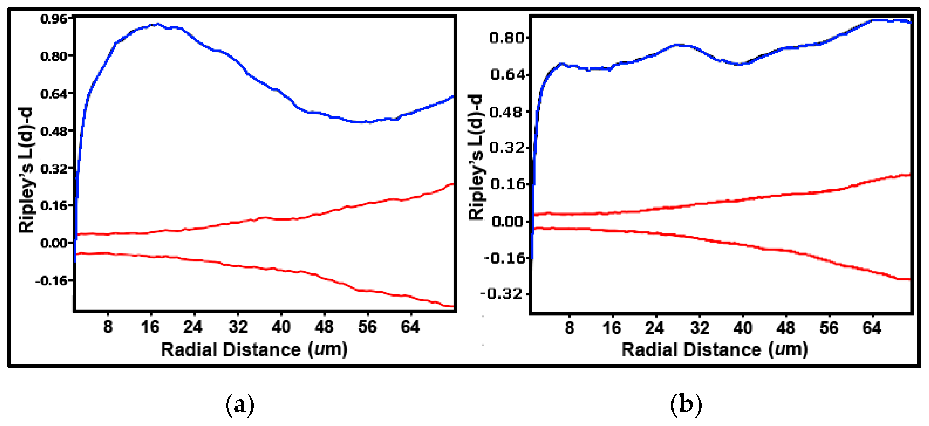
A useful counterpart to these point-pattern analyses is the Ripley’s K multi-distance clustering analysis [5,42,71]. This second-order, point distribution statistic interprets multiple separation distances between objects to determine point pattern changes over a wide spatial scale [5,71]. K(d)-d measures average object counts within circles with a distinct radius d centered on every object point in the landscape divided by the mean spatial density of all objects present [42,71]. A plot of K(d)-d vs. all radial separation distances in the landscape indicates uniform, random or clustered dispersion patterns determined by a Monte Carlo simulation of the 95% confidence interval representing the critical limits of complete randomness [42]. K(d)-d values indicate overdispersed, uniform distribution patterns when located below the confidence envelope, and clustered distribution patterns when located above the envelope [42,71]. Peaks of K(d)-d values exhibiting the most intense aggregation can also be scrutinized at definable radial separation distances [5]. The Ripley K plots over the same sampling interval range for both landscapes showed strong spatial structures with a uniform pattern at only one short radial distance, and clustered patterns above the 95% confidence envelope for the remaining 99 greater radial distances examined (Figure 14a,b). Spatially aggregated patterns for cells in biofilm community A on plain glass had one peak of K(d)-d at a radial distance of ~16 μm (Figure 14a), whereas cells in biofilm community B on polystyrene exhibited multimodal peaks of K(d)-d at radial distances of ~7, 30, and 66 μm (Figure 14b).

Five additional methods of single-cell analysis were performed to capture the spatial relationships between neighboring cells and gain further insight on the predicted intensities of their in situ cell–cell interactions and colonization behaviors on different substrata. These analyses examined their fractal dimension, point kernel density, minimal spanning tree, linear point alignments, and geostatistical autocorrelation of pertinent z-variates.

Fractal analysis of structured biofilms can discriminate self-similar spatial patterns of biomass and deliver insights on intensity of cooperative microbial interactions, including their efficiency in positioning for optimal utilization of fractal-like apportionments of resource distributions and coexistence of multiple species among community members [5,7,15,25,26,27,30,31,32]. A box counting analysis [15] of inverted binary montage images (e.g., Figure 1g,h) indicated that the spatial pattern of individual cells in biofilm community B had a greater fractal dimension (mean ± std. dev. of 1.115 ± 0.046 compared to 1.019 ± 0.058 for community A) that was statistically significantly (Student t of 2.562, p same mean of 0.04). This greater fractal dimension of individual cell distributions in the biofilm community B indicates that they have higher spatial complexity, are responding to significantly different ecological processes that control their spatial structure on the polystyrene substratum, and predictably reflect an increased, fractal-like nutrient apportionment in that landscape [15,25,26,27].

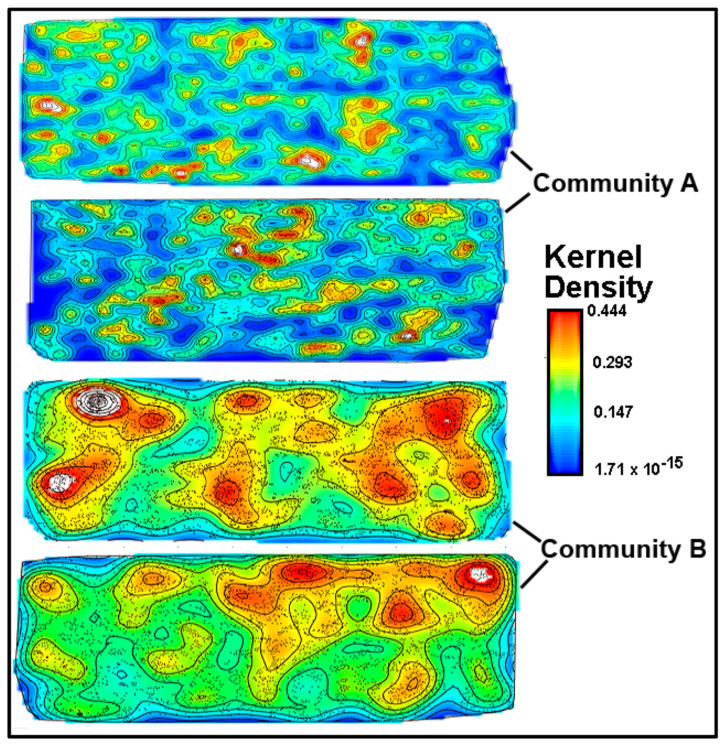
A kernel density analysis [42] was performed on the data of spatial point coordinates to examine the in situ density of cells in both community landscapes. This spatial mapping tool uses a Gaussian smoothness method to estimate the probability of (dis)continuity in gradients of local cell density interpolated over the landscape area [42]. Figure 15 shows equivalent pseudocolored scalings of spatial point kernel densities for cells in high-resolution montage images of the two river biofilm communities. A comparison of the landscape domains clearly reveals differences in the heterogeneity and discontinuity of georeferenced spatial intensity of the clustered cells in situ. Cells in community B congregated into several foci with greater kernel point densities that were spread over larger regions of the biofilm landscape, and had higher gradient connectivity with less discontinuity of kernel densities compared to cell locations in the biofilm of community A. Kernel densities of cells in community A had more discontinuity, as indicated by numerous internal gradients of aggregation that diminished to the minimum (blue) density within the full range present.

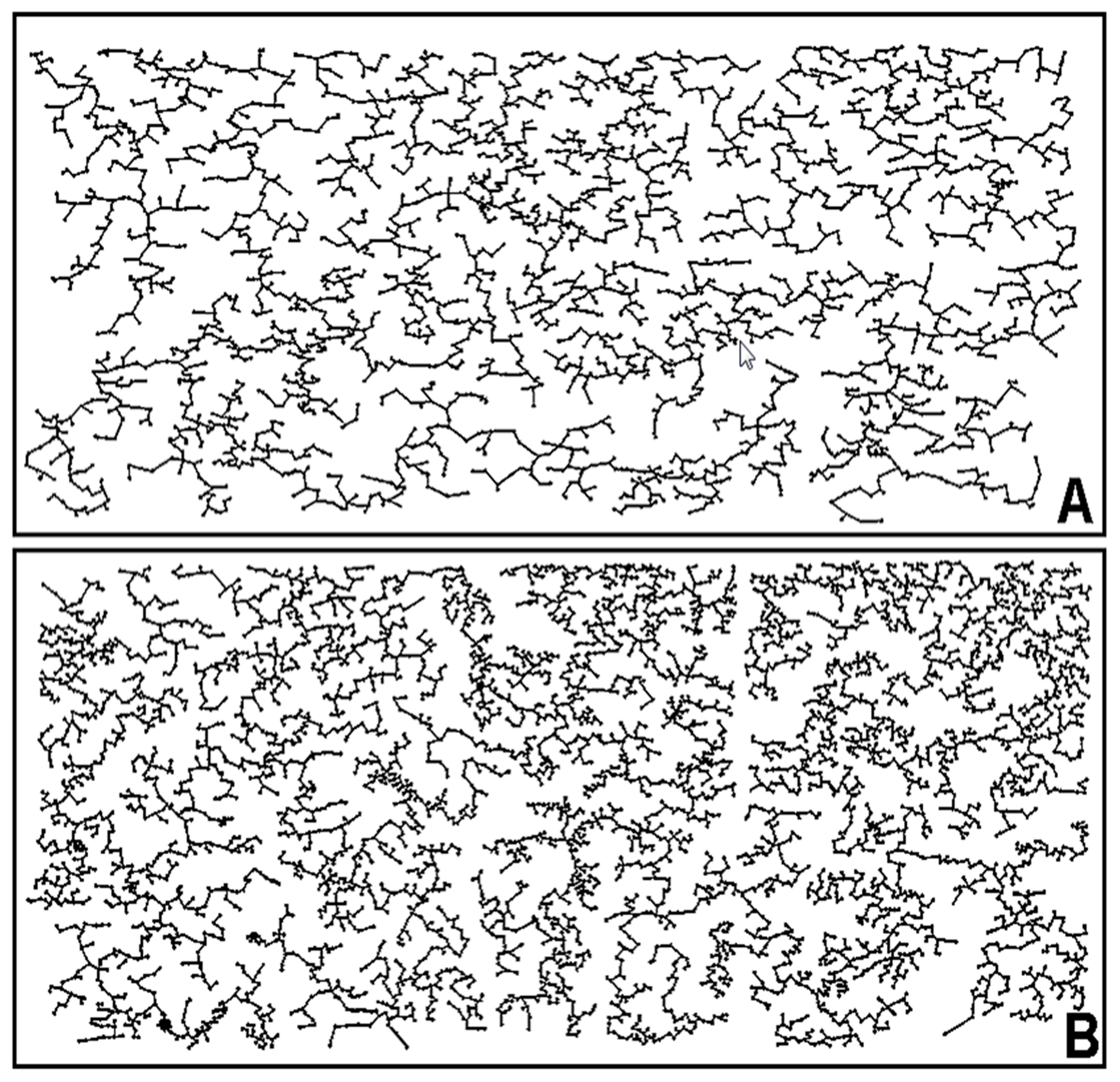
Analysis of the minimal spanning tree is another powerful guide to envision predicted opportunities of cell–cell interactions based on statistical analyses of the spatial connectivity between individual community members within the landscape [77]. This method of spatial analysis creates a subgraph image of the original landscape with each cell point linked by the shortest linear vertex to its closest neighbor, ultimately producing a nearest-neighbor network of vertices inevitably connecting all cells to each other in a single tree with a multi-branched architecture having minimum total length and containing no closed loops [27,42]. Visual inspection of the tree reveals local aggregated patches where increased densities of vertices with short lengths predict high probability of intense cell–cell interactions. Minimal spanning trees derived from nearest neighbor point analysis of representative montage images of biofilm communities A and B (Figure 1i–j) are presented in Figure 16A,B. The minimal spanning tree of community B provides a vivid representation of greater connectivity among many more patch areas with branched vertices of shorter length.

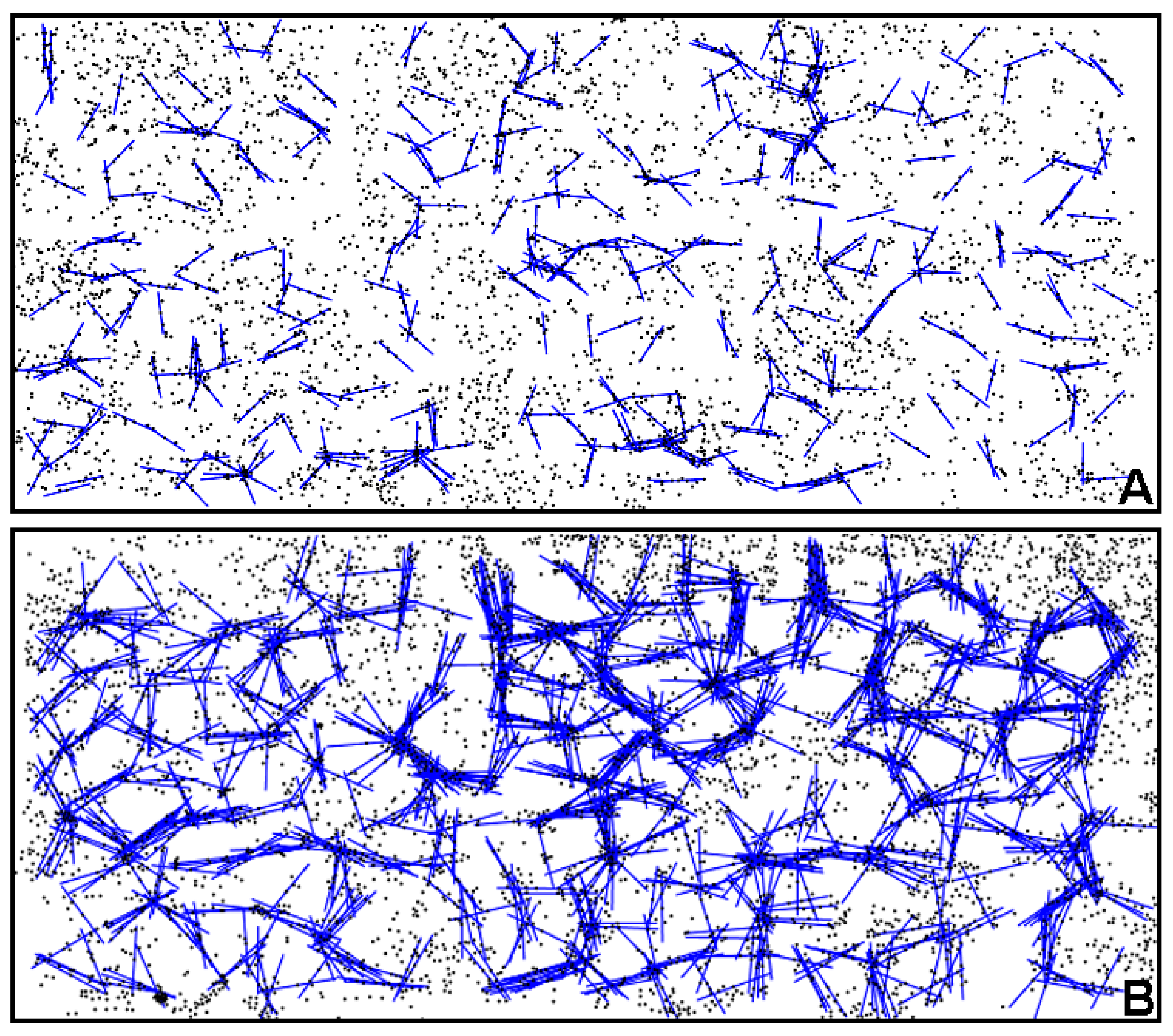
Further indications of the spatial location of intense cell–cell interactions are provided in two-dimensional directional plots that use a continuous sector method to transform individual object point positions noted by their Cartesian coordinates into another domain of statistically significant, linear alignments within the landscape [5,42,78]. 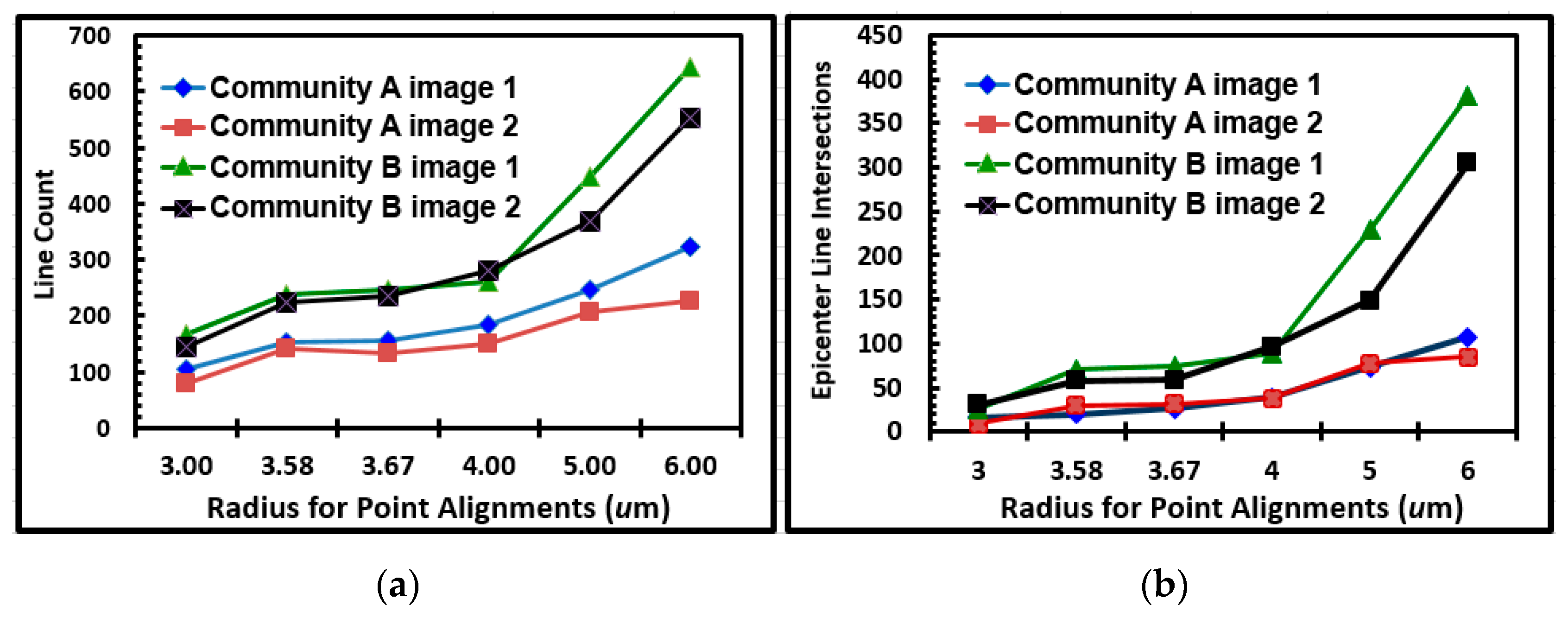Plots of linear point alignments computed at equivalent sampling intervals for river biofilm communities A and B are presented in Figure 17A,B, respectively. These results indicated many linear alignments whose multi-directional angular orientations identified more “hot-spot epicenters” of interpoint intersections created by intense clusters of closely neighboring bacteria in the community B developed on the polystyrene substratum. Quantitative assessments of the number of linear alignments and their epicenters of clustered intersections confirmed their increased intensities for community B over a range of increasing radial distances of sampling (Figure 18a,b). These results provide additional evidence supporting the hypothesis that cell–cell interactions are predictably more abundant and intense within the spatially clustered patterns of cells in the community B biofilm developed on the polystyrene substratum.

The final method of spatial ecology analysis for this study involved a geostatistical approach that measures the dependency among z variate observations in georeferenced space in order to evaluate the continuity or continuous variation of spatial patterns over that entire landscape domain [5,7,44,72]. It does so by quantifying the resemblance between z variate values at neighboring points as a function of their spatial separation distance [5,7,44,72]. The data indicate positive autocorrelation if the z variate values of neighboring pairs are more similar when located nearby rather than far apart [5,72], as occurs when communities are spatially clustered to facilitate cell–cell communication and cross-feeding [9,38,62]. When found, autocorrelated z variates are then mathematically modeled using regionalized variable theory to connect various spatially dependent relationships of their ecology, including the range of real-world radial distances at which they occur in situ [44,68,72].

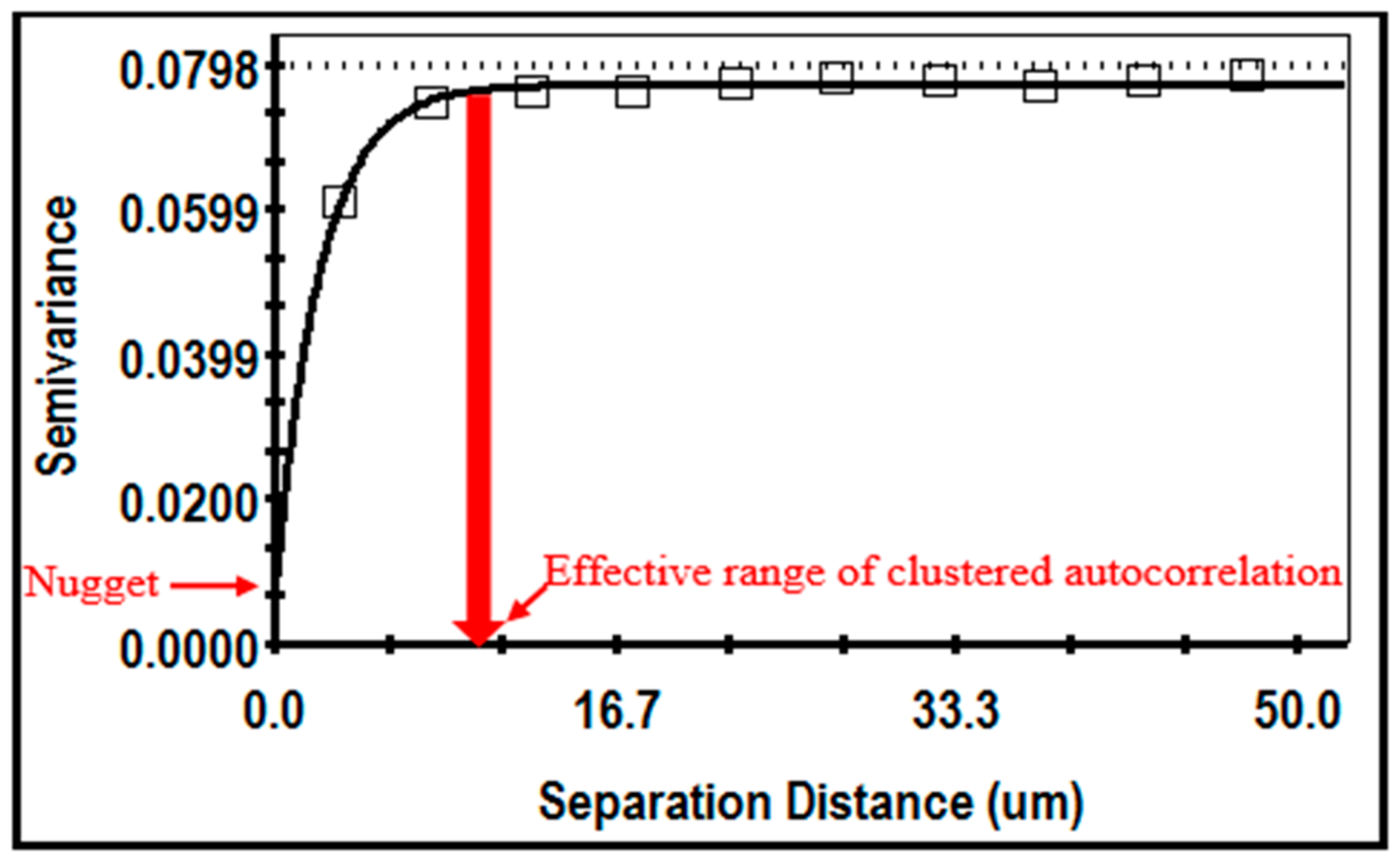
Geostatistical analysis produces a semivariogram (Figure 19) describing the extent that the measured z variate exhibits autocorrelated spatial dependence between all cell pairs at multiple sampled locations [5,7,68,72]. Spatial autocorrelation of two z variates were evaluated in this study: a CMEIAS cluster index indicating the intensity of aggregated colonization behavior between nearest cell neighbors [5,45], and the cell biovolume to test for cell–cell interactions among neighbors affecting their allometric metabolism and growth ecophysiology [5,10,37]. For microbial biofilm analyses, these two z variates typically have units of μm⁻¹ and μm³, respectively.

Figure 19 shows an example of the isotropic semivariogram for the cluster index of cells in a montage image of the biofilm community B. Important discriminating features include the nugget at the Y-axis intercept denoting the amount of measured microstructure that is not spatially dependent, and the effective separation range indicating the X-axis value at 95% of the model’s asymptote height, representing the maximal separation distance between sampling points at which the z variate is still autocorrelated [5,7,68,72]. This example indicates a strong spatial autocorrelation of the cluster index, with a very small nugget (sufficient points have been adequately sampled) and the autocorrelated effective range that defines the maximal radial distance between cells that still influences their neighbor’s ability to congregate locally in situ within the defined spatial domain. Geostatistical tests for geometric anisotropy in the semivariograms at 0, 45, 90, and 135 compass degrees did not indicate a preferential bias in directionality of cells in the biofilms, suggesting no major directional influence of hydrodynamic forces exerted on their cell positioning during development of the biofilms within the gently flowing river.

Table 17. Spatially autocorrelated z variates of cluster index and cell biovolume for river biofilm communities A and B developed on plain glass and polystyrene substrata, respectively.

Community (Image No.)	Autocorrelated Z Variate	Model Fit (Residual SS)	Nugget	Effective Range (μm)	% of Cells within Effective Range
A (No. 1)	Cluster Index	2.06 × 10−4	0.0109	6.6	100
A (No. 2)	Cluster Index	3.98 × 10−4	0.0092	6.6	100
B (No. 1)	Cluster Index	1.45 × 10−6	0.0026	10.8	100
B (No. 2)	Cluster Index	3.83 × 10−5	0.0086	9.6	100
A (No. 1)	Biovolume	1.64 × 10−2	0.0410	6.9	96.46
A (No. 2)	Biovolume	4.71 × 10−5	0.0009	6.6	96.47
B (No. 1)	Biovolume	1.08 × 10−1	0.0748	11.6	99.94
B (No. 2)	Biovolume	2.45 × 10−4	0.0022	12.3	99.89

summarizes the geostatistical analyses of the cluster index and biovolume z variates for equal sampling efforts of individual cells in the two biofilm community landscapes. Both biofilms exhibited spatially-dependent isotropic autocorrelation for both z variates. Their nugget variances were small, indicating that the analyses were adequately sampled with little discontinuity of small-scale variation, and the majority of their measured microstructure was spatially autocorrelated. The exponential model made an acceptable fit (low residual sum of squares) to the semivariogram data for both community z variates. Two-tailed Student t and Mann–Whitney tests indicated that the cluster index for cells in community B had significantly greater mean and median values (p of 1.52 × 10⁻¹⁴¹ and 0.000, respectively). In addition, the effective separation ranges for both autocorrelated z variates were somewhat longer (hence stronger) with the biofilm community B developed on the polystyrene substratum (statistically significant for biovolume). Most cells in both communities had nearest neighbor distances that positioned them well within the corresponding specific effective ranges of influence, and thus their “socially-adapted” proximity to each other was sufficient to enable spatially autocorrelated cell–cell interactions affecting these ecophysiologically relevant metrics. These geospatial analyses provide statistical proof of spatially structured biofilm communities with predominantly aggregated distribution patterns that exhibit positive cooperative interactions between proximal cells benefitting their colonization and productivity, and also reveal the real-world spatial dimensions at which these cell–cell interactions extend in situ.

4. Summary and Conclusions

This paper describes many applications of computer-assisted microscopy using CMEIAS bioimage informatics software to perform a comprehensive in situ analysis of river biofilm ecology, thereby advancing our understanding of this major lifestyle for microorganisms. The study compared two river biofilm communities developed on contrasting substrata (plain borosilicate glass vs. polystyrene polymer) with significantly different physicochemical properties, used optimized settings of digitally processed images, their threshold segmentations, and spatial scales to perform phenotypic analyses of microcolony biofilms and individual cells at appropriate resolutions. The many examples described here illustrate how two-dimensional images of natural immature biofilms can be acquired using conventional transmitted brightfield and phase-contrast microscopy before the substratum is significantly covered with cells embedded within a confluent matrix, and then be analyzed to extend the range of biofilm architectural and ecological characteristics beyond common three-dimensional analyses using images acquired by multi-channel laser scanning confocal microscopy.

Many quantitative features were extracted from digital images of these foreground objects to investigate their size, abundance, surface texture, contour morphology, fractal geometry, morphological diversity, ecophysiology, and landscape/spatial ecology. The results of numerous discriminating statistical tests that take into account the variation in replicated samples indicate that river biofilm architecture exhibits significant geospatial structure in situ. These provide many insights on the strong influence that substratum hydrophobicity vs. wettability exerts on biofilm development and ecology at spatial scales in the micrometer range that are directly relevant to their ecological niches. Important physicochemical properties controlled by these contrasting surface characteristics that would influence microbial colonization behaviors at the glass–water and polystyrene–water interfaces include the adsorption/dispersion/apportionment of nutrient resources, development of a conditional surface water layer, free energy of water displacement during cell adsorption and relocation, primary and secondary energy minima and other attractive-repulsive forces distinguishing hydrophilic-hydrophobic interactions in aqueous environments [22,23,79]. This collective information should be considered when designing and interpreting experiments that use polystyrene as the colonization substratum to identify the molecular and cellular requirements for biofilm development [5].

Despite both biofilm assemblages being derived from the same natural bacterioplankton community in the flowing river ecosystem, numerous test results provided compelling evidence indicating that the biofilm community B developed on the polystyrene substratum was the recipient of “higher rewards.” These benefits resulted in its significantly greater overall ability to convert locally available resources into biomass, build enhanced architectural complexity/connectivity/dispersion, increase morphotaxa diversity, and intensify numerous other ecologically important features indicative of improved positioning of its colonization pattern for optimal apportionment of fractal-like distributions of limiting nutrient resources, increased allometric metabolic rate and adaptive responses to predator bacteriovory stress, and produce a higher abundance of spatially structured patches of aggregated patterns that would enable stronger, positive, cooperative, autocorrelated cell–cell interactions benefitting their productivity, as predicted [5,10,15,25,26,27,28,29,30,31,32,33,34,35,36,37,38,48,49,50,51,52,56,57,58,59,60,61,62,72,73,74]. Community A had lower intensities for these phenotypic characteristics, plus a smaller morphotype diversity due to higher dominance (less evenness) of its coccus morphotype class and indication of stronger adaptive responses to starvation stress within its biofilm. These many contrasting features of the two microbial communities indicate that they followed dissimilar paths of biofilm development on these substrata in the same river ecosystem.

Many metrics of bioimage informatics used in this work are able to discriminate biofilm architecture, ecophysiology and biogeography. This study provides the workflow direction, optimized methods of data acquisition and analysis of statistical significance, and ecological interpretations of test results that are strongly embedded in ecology in general and provide evidence of their enhanced productivity, connectivity, edge boundaries and shape complexities with greater fractal dimension that create opportunities of strong social colonization behavior promoting their further expanded growth [5,9,10,15,25,26,27,28,29,30,31,32,33,34,35,36,37,38,61,62]. This collection of technologies complements other direct and indirect methods to measure the physical forces of microbial adhesion to abiotic surfaces [79]. In addition, including image analysis enables the user to quantitatively differentiate the ecologically important spatial patterns of microcolonies and individual cells in microbial biofilms rather than just report a qualitative description of a “clumpy” or “dispersed” landscape [16,56].

We conclude that substratum physicochemistry significantly impacts on the early immature stage of biofilm development in river ecosystems, and that bioimage informatics can fill major gaps in understanding the geomicrobiology and microbial ecology of biofilms when examined in situ at suitable spatial scales before they become confluent. This study also illustrates how CMEIAS computer-assisted microscopy performed at single-cell resolution can contribute useful information supporting contemporary studies that seek to understand bacterial individuality in order to test the emerging theory of individual-based modeling and ecology, which predicts that single cell variation is a major driver of evolutionary events and the ecological dynamics of population structure and function [5,61,80,81,82].