
Surface State across Scales; Temporal and Spatial Patterns in Land Surface Freeze/Thaw Dynamics †


1
Department of Geoinformatics, University Salzburg, 5020 Salzburg, Austria
2
Arctic Centre, University of Lapland, 96200 Rovaniemi, Finland
3
Zentralanstalt für Meteorologie und Geodynamik, 1190 Vienna, Austria
4
Austrian Polar Research Institute, 1010 Vienna, Austria
5
b.geos, 2100 Korneuburg, Austria
*
Author to whom correspondence should be addressed.
†
This paper is an extended version of our paper published in Helena Bergstedt, Annett Bartsch (2016): Surface Status Across Scales. Proceedings of the ESA Living Planet Symposium, Prag, Czech, May 2016
Geosciences 2017, 7(3), 65; https://doi.org/10.3390/geosciences7030065
Submission received: 30 April 2017
/
Revised: 22 July 2017
/
Accepted: 25 July 2017
/
Published: 3 August 2017
(This article belongs to the Special Issue Cryosphere)
Abstract
:Freezing and thawing of the land surface affects ecosystem and hydrological processes, the geotechnical properties of soil and slope stability. Currently, available datasets on land surface state lack either sufficient temporal or spatial resolution to adequately characterize the complexity of freeze/thaw transition period dynamics. Surface state changes can be detected using microwave remote sensing methods. Data available from scatterometer and Synthetic Aperture Radar (SAR) sensors have been used in the past in regional- to continental-scale approaches to monitor freeze/thaw transitions. This study aims to identify temporal and spatial patterns in freeze/thaw dynamics associated with the issue of differing temporal and spatial resolutions. For this purpose, two datasets representing the timing of freeze/thaw cycles at different resolutions and spatial extents were chosen. The used Advanced SCATterometer (ASCAT) Surface State Product offers daily circumpolar information from 2007–2013 for a 12.5-km grid. The SAR freeze/thaw product offers information of day of thawing and freezing for the years 2005–2010 with a nominal resolution of 500 m and a temporal resolution of up to twice per week. In order to assess the importance of scale when describing temporal and spatial patterns of freeze/thaw processes, the two datasets were compared for spring and autumn periods for the maximum number of overlapping years 2007–2010. The analysis revealed non-linear landscape specific relationships between the two scales, as well as distinct differences between the results for thawing and re-freezing periods. The results suggest that the integration of globally available high temporal resolution scatterometer data and higher spatial resolution SAR data could be a promising step towards monitoring surface state changes on a seasonal, as well as daily and circumpolar, as well as local scale.
1. Introduction
Permafrost and seasonal frost-related phenomena affect large parts of the Earth’s surface and are therefore important variables in climate research. This is especially true for Arctic areas where the ground surface undergoes a yearly freezing and thawing cycle. Transitional periods play a special role in the Arctic ecosystem; they can last several weeks, and changes in their duration and intensity have been found to have significant impact on terrestrial carbon exchange and changes in ecosystem productivity [1,2]. The freezing and thawing process has also been linked to hydrological processes like surface runoff [3], geotechnical properties of soil [4], biogeochemical properties of thermokarst lakes [5] and slope stability in alpine regions [6]. In addition, freeze/thaw cycles are known to influence methane emissions [7]. Therefore, their spatial extent, as well as changes in their dynamics have implications for hydrological applications, climate modeling and ecosystem processes [8], which occur at different scales. Regions underlain by permafrost are of special interest in this context as they have been shown to undergo rapid warming [9,10,11,12], and changes in ground stability have direct implications for roads, buildings and other forms of infrastructure [13]. Currently available datasets describing the freeze/thaw state of the ground surface lack either the adequate spatial or temporal resolution to describe these processes on a regional/local scale [14].
The surface state of the ground can be monitored using microwave remote sensing [15]. Brightness temperature or backscatter varies due to changes in dielectric properties when water changes from liquid to solid and vice versa. The water contained within the soil therefore influences the signal. The dielectric constant of water changes substantially when it freezes. The change in the dielectric constant results in a response of the backscatter signal or brightness temperature respectively, and it can therefore be used to detect the timing of the status change of land surfaces [1].
A further advantage of microwave sensors is that microwave radiation can penetrate cloud cover and is independent from the presence of daylight. Satellite data have been applied in several studies to detect the state of the ground surface using active microwave and passive microwave sensors (e.g., [16,17,18,19]). At C-band, the presence of snow can be a complicating factor during surface state retrieval [20]. Melting snow causes backscatter variations, which are different from those caused by the thaw of snow-free land surfaces [21]. When soil thaws, the liquid water content increases, and therefore, the backscatter coefficient under snow-free conditions increases, as well [15]. In snow-covered areas, the backscatter drops with the onset of snow melt due to the diminished effect of volume scattering and the presence of shallow water ponds at the snow surface [20,22]. This effect enables the monitoring of snow cover parameters, e.g., [23,24,25,26,27,28,29], and the characteristics of sea ice [30,31,32,33].
A further issue is the wavelength. Different wavelengths have been tested for freeze/thaw retrieval. The interaction of the microwave signals with the ground surface differs, influencing their suitability for freeze/thaw retrieval. Freeze/thaw products exist from L-band (e.g., [34]), C-band (e.g., [20,35]) and at 37 GHz (in the case of the Special Sensor Microwave Imager (SSM/I)) (e.g., [36]) observations. Longer wavelengths, such as L-band, are considered as most suitable for freeze/thaw application due to the potentially higher penetration depth into the soil [17,37,38]. Data from active systems are available from scatterometer (real aperture) and Synthetic Aperture Radar (SAR). Scatterometer data hold the advantage of a high temporal resolution and have a good coverage of the Arctic due to overlapping orbits, yet the spatial resolution of scatterometer data is comparatively coarse. C-band scatterometers have been shown to have the capability for monitoring the freeze/thaw conditions of the ground surface and have been successfully used to map surface state conditions on a circumpolar scale [20]. However, due to their lack of high spatial resolution, scatterometer data are suspected to be insufficient to describe freeze/thaw processes on a local scale. The coarse spatial resolution holds further disadvantages during transitional periods as the ground covered by one scatterometer footprint is likely a mixture of frozen and thawed ground and not a homogeneous area, as implied by the coarse resolution data [20]. An advantage of active systems is that they can also provide observations in higher spatial resolution using SAR systems.
SAR has been shown to be a useful tool for monitoring of the surface state and other ground surface properties on a finer spatial scale by several studies (e.g., [35,39,40]). Furthermore, outside of freeze/thaw detection, especially C-band SAR has been used to complement data provided by scatterometer sensors during unfrozen conditions [21]. However, it does not provide the global coverage and temporal resolution that can be achieved by scatterometers.
The scarcity of suitable high resolution SAR datasets for the Arctic region prevents monitoring of freeze/thaw cycles with adequate spatial and temporal resolution. This would be especially crucial during transition periods when changes in surface state can occur on a daily basis. Freeze/thaw products with high spatial resolution are only available from C-band and for selected regions (e.g., [41]), while circumpolar datasets are derived from coarse resolution data from both active sensors like the Advanced SCATterometer (ASCAT) (C-band, 25-km spatial resolution; e.g., [20,42]) and passive sensors like SMOS (L-band, 35–50-km spatial resolution; e.g., [17,43]). The Soil Moisture Active Passive (SMAP) mission was expected to solve this problem [44], but its failure has left this gap open. Efforts to enhance the spatial resolution of scatterometer data exist [45], but freeze/thaw products with both high temporal and spatial resolution are not yet available. This could be overcome by downscaling coarse resolution scatterometer data using additional information such as topography, landscape type, vegetation or the climatological parameter. The lack of knowledge about the relationships of processes detectable at different scales prevents such efforts until now [14]. Park et al. [35] provide initial analyses of the influence of forest on step function-based C-band freeze/thaw detection. They conclude that the canopy plays a significant role. Högström et al. [21] quantify the impact of lake backscatter variations within the ASCAT footprint using ASAR wide swath data (150 m) for soil moisture retrieval, e.g., wind can cause an increase of 5 dB in areas with 50% water fraction.
In this study, we analyze the spatial and temporal relationships between freeze/thaw processes detectable at different scales. We employed two freely-available data products that are based on C-band radar observations. They were derived from the ASCAT on board the MetOp satellite and the Advanced Synthetic Aperture Radar (ASAR) sensor on board ENVISAT, a scatterometer and SAR sensor, respectively, which deliver surface state information at different temporal and spatial resolutions. The general objective of this study was to explore these relationships for different landscape types and the representativity of coarse resolution scatterometer data for different permafrost environments.
2. Materials and Methods
The data products from the ASCAT and and ASAR sensors describe the surface state of Arctic environments for differing extents at different spatial and temporal resolutions.
The first data product provides daily information on the freeze/thaw condition of the ground surface on a circumpolar scale. It was derived from data obtained by the ASCAT sensor (C-band) on board the meteorological MetOp satellite (A and B) [20,42]. ASCAT incidence angles range between 25° and 65°. They were normalized to 40° [20] before further processing. The dataset contains classes that reflect daily surface state information for the area above 55° N with a spatial resolution of 25 km × 25 km, gridded to 12.5 km, for the time period of January 2007–December 2013 [42,46]. The surface state has been determined by applying an empirical threshold algorithm. The threshold was determined for each single grid point in order to especially account for the impacts of vegetation. A certain class (frozen, melting snow, unfrozen) has been assigned to each measurement [20]. Unfrozen refers here to the condition without snow cover. The accuracy of the algorithm is highest in summer and winter and lowest during spring and autumn [20]. The classification accuracy has been tested using air temperature measurements from the nearest World Meteorological Organization (WMO) stations, as well as surface temperature data from GLDAS-Noah [47] and ERA-Interim reanalysis datasets [48]. It was found to be above 80% overall [20].
The second product was derived from data obtained by the ASAR sensor on board the European environmental satellite ENVISAT operating at C-band. The dataset covers five regions (Alaska, Mackenzie, Laptev Sea Coast, Central Yakutia and Ob Estuary, Figure 1) and gives information about the day of thawing and freezing for the time period of 2005–2010 [41,46]. The information is given at a spatial resolution of 1 km and provided with a nominal resolution of 500 m. The classification accuracy is < weeks for freezing and weeks for thawing [41]. The used mode (global mode) is characterized by varying incidence angles (ranging between 20° and 40°) and high noise, making a threshold function not applicable. Data were normalized to 30°, and a step function has been fit for each location to all available measurements of a year [35]. The points in time for the change (increase of backscatter to the level of unfrozen and snow free conditions and decrease for freeze-up) have been extracted, resulting in two images per year with the day of thaw and day of freeze-up as values. A third band provides the number of ASAR acquisitions that was available and used in the creation of the data product for each year. In general, all pixels with less than 52 acquisitions are masked. The data product was validated using meteorological data, such as air temperature and snow water equivalent [35]. The agreement in spring and autumn was found to be 90.6% and 87.5%, respectively. The accuracy is linked with the temporal frequency of the input data [35], which varies between the regions and the covered years and is documented in the dataset. Other factors influencing the accuracy are land cover heterogeneity and frost action dynamics [35]. In their study, Park et al. [35] show an increase of uncertainty with a decrease of temporal resolution of the input data. Pixels containing values believed to be unreliable were masked out; this includes pixels with low coverage (less than 52 ASAR GM acquisitions per year), as well as pixels containing water bodies.
Acquisitions from ascending, as well as descending orbits are available from both ASAR and ASCAT. The time of day for ascending and descending orbits is different, and measurements are either from the morning or afternoon. This may lead to different results (frozen or unfrozen) for a certain day due to daily temperature variations. The melting snow class in the ASCAT product has not been considered as unfrozen for the purpose of this study, although the ground below may start to thaw when snow is melting [49]. First, the detection of melting snow for a certain day depends on actual acquisition timing (a.m. or p.m., not all days with melting might be captured), and second, melting snow is not available from the ASAR product as it only gives information on the day of year of the freeze and thaw. Even though ASCAT and ASAR have different incidence angles, the results are assumed to be comparable. The change from frozen to unfrozen can be considered similar to the change from moist to dry. This has been demonstrated to be almost incidence angle independent [50].
Both algorithms (the one used for ASAR and the one for ASCAT) identify unfrozen ground surface when a certain backscatter intensity (distinct from the winter values) is reached that corresponds to summer values [20,35]. This value is higher than in winter and even much higher than under conditions of snow melt. ASAR therefore corresponds in general to end of snow melt. Park et al. [35] found that this differs for forested areas. Here, it corresponds to the beginning of snow melt. This is one of the reasons that forested areas are analyzed separately in this study.
We analyzed discrepancies on a regional scale, using the extent of the SAR product. We studied the years 2007–2010, as this is the time period covered by both datasets. To enable the comparison of the two datasets, the SAR product was transferred from information of the day of freeze and day of thaw into daily values of the freeze/thaw surface state for each 500-m pixel. Days after the recorded thaw date were classified as thawed, all days before as frozen (respectively for days before and after the freeze date). To further facilitate the comparison, the coarse ASCAT product was resampled to the 500-m grid of the SAR product without losing information through interpolation. We then checked the agreement and discrepancy days for each ASCAT grid cell for the years of 2007–2010, comparing the results to the number of acquisitions that went into the creation of the SAR product. Discrepancy days on the regional level were calculated as the number of days the two data products did not report the same surface state. This includes incidences where pixels are masked. In the case of the SAR product, this occurs due to data unavailability or lake fraction, in the case of the ASCAT dataset, especially when the surface is classified as melting snow. It does not distinguish between the different forms of discrepancy that are described in Figure 2. To demonstrate the relationship between discrepancies and terrain, we compared the discrepancies to a topographical map.
To investigate possible relationships in greater detail, we identified 15 ASCAT grid cells for different landscape types. Four different landscape types (forest, tundra, lake dominated tundra, tundra with partial floodplain) were determined using the Global Land Cover 2000 (GLC2000) datasets for North America [51] and Northern Eurasia [52]. The grid cells were selected in regions with lower than 50% masked SAR pixels in all 4 years to guarantee meaningful results. Grid cells were chosen in the regions Alaska (A), Mackenzie (B) and Laptev Sea Coast (E) (see Figure 1). The regions Central Yakutia (D) and Ob Estuary (C) were not selected due to missing values for the day of thaw in Region D in 2009 and the low number of SAR acquisitions in Region E in all years (see Figure 3). Due to the low number of acquisitions, all pixel in Region C failed the condition of lower than 50% masking per grid cell for at least one of the 4 years. All selected grid cells also have similar average transition times as determined in [20] and are limited in elevation range (on average, 150 m). Due to the constraints of these criteria, areas containing suitable grid cells were limited. This led to all selected grid cells being located in continuous permafrost environments as defined by Brown et al. [53] and an uneven distribution of certain landscape types across the regions. Using these grid cells as our study area extent, we repeated the analysis already done on a regional level with a special focus on transitional periods. We compared spatial and temporal patterns for spring and autumn, as well as the percentage of frozen SAR pixels at the point of the surface state change reported in the ASCAT dataset. We further divided the grid cells into four classes of landscape types (forest, tundra, lake dominated tundra, tundra with partial floodplain).
To investigate the spatial and temporal variability of discrepancies between the data products, the following statistical measures have been derived. A 4-year mean value for days of discrepancy was calculated for each ASAR pixel for the years 2007–2010. Unlike the discrepancy days for the regional analysis, all analyses on the grid cell level were done excluding masked SAR pixels from the calculations. This focuses the analysis on the discrepancies between frozen and unfrozen (see Figure 2 for types of discrepancies). To achieve this, all SAR pixels that were masked at least once in the data product were masked for our analysis. For the transitional periods, we analyzed the percentage of already thawed/frozen SAR pixels within each ASCAT grid cell with respect to the surface state reported by the ASCAT product. To quantify the spatial variability within each grid cell in spring and autumn, we calculated the standard deviation of discrepancies, taking into account all grid cells that were not masked in the years 2007–2010. The differences between landscape types were assessed and visualized using box plots of the percentage of frozen and thawed SAR pixels per ASCAT grid cell at the time of the surface state change reported in the ASCAT product. The influence of the number of SAR acquisitions considered in the freeze/thaw product on the number of discrepancy days was explored, calculating the median for both parameters for each grid cell for spring and autumn for each year separately.
For a more detailed analysis of temporal patterns, we used air temperature and near-surface soil temperature data from a measurement station located within the Alaska 2 grid cell [54,55]. It is the only cell with available in situ records. We compared the in situ measurements to the ASCAT surface state and the SAR surface state. To mitigate the effect of artifacts in the SAR product and to account for its resolution of 1 km, we chose the maximum value of the four closest pixels (4 × 4 pixel window). The measurement station is located on a slope that increased the number of artifacts in the vicinity.
3. Results
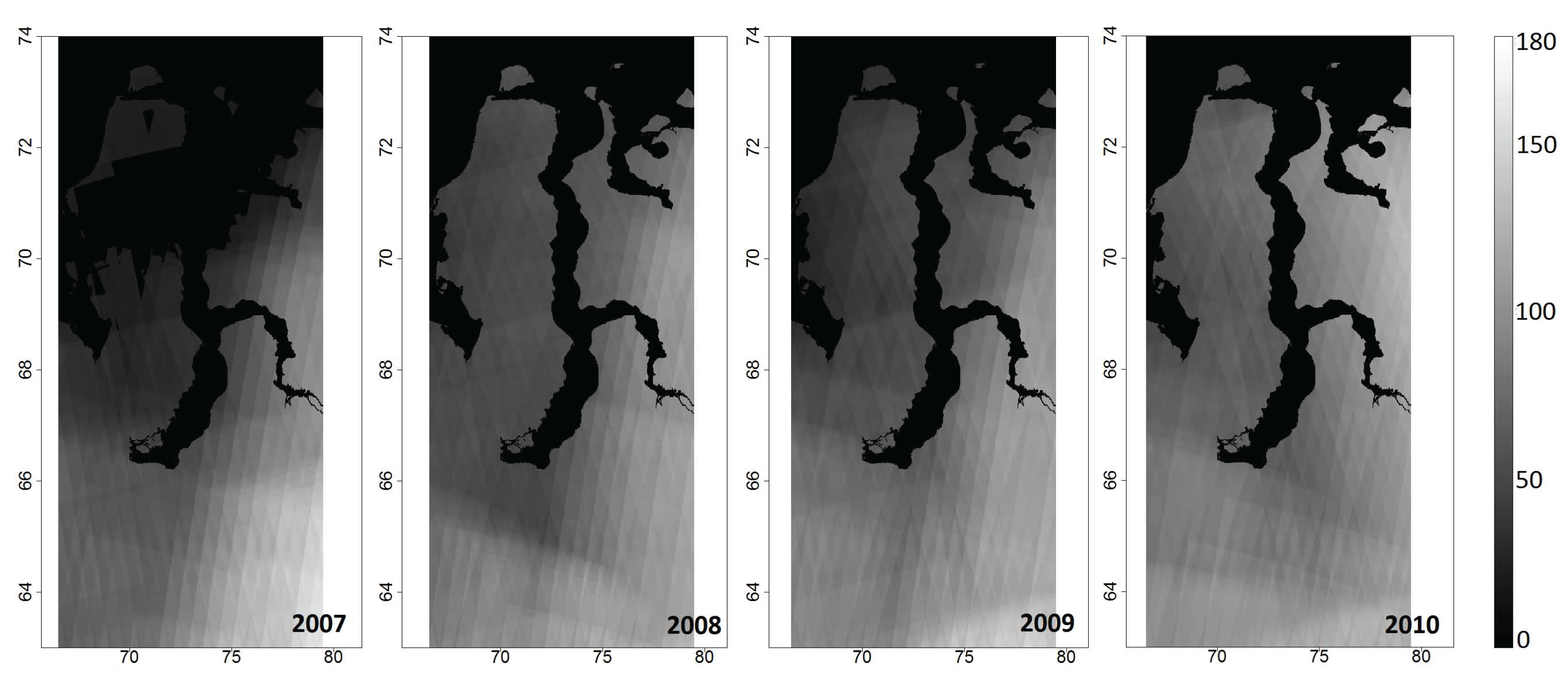
The analysis of discrepancies on a regional level revealed spatial and temporal patterns that underlined the need for further analysis on a pixel level (Figure 4, Figure 5 and Figure 6). Higher differences occur for mountainous regions and lake-rich environments. Landscapes of a more homogeneous nature show in general fewer discrepancy days. Figure 7 exemplifies the high discrepancy day values in mountainous areas. Large proportions of the Alaskan and Canadian subsets are characterized by mountain regions. The different regions show regional mean values of discrepancy days (spring and autumn all four years) from 96.3 days (Central Yakutia) to 192.3 days (Ob Estuary), meaning that the discrepancies extend beyond transitional periods. In the case of smooth terrain, this difference is mostly less than one month. Discrepancies between the two datasets are influenced by the number of acquisitions considered in the SAR dataset (see Figure 3 and Figure 5). The Ob Estuary region acts as a good example for the importance of temporal resolution. The region (as seen in Figure 3) has a low number of acquisitions considered in the SAR dataset. It is also the region with the highest spatially consistent number of discrepancy dates. There is a gradient of acquisition numbers from southeast to northwest, which leads to a similar gradient in discrepancy days. The northern part of the Alaskan subset is also affected by a lower number of used SAR acquisitions. The number of discrepancy days more than doubles north of 70° N.
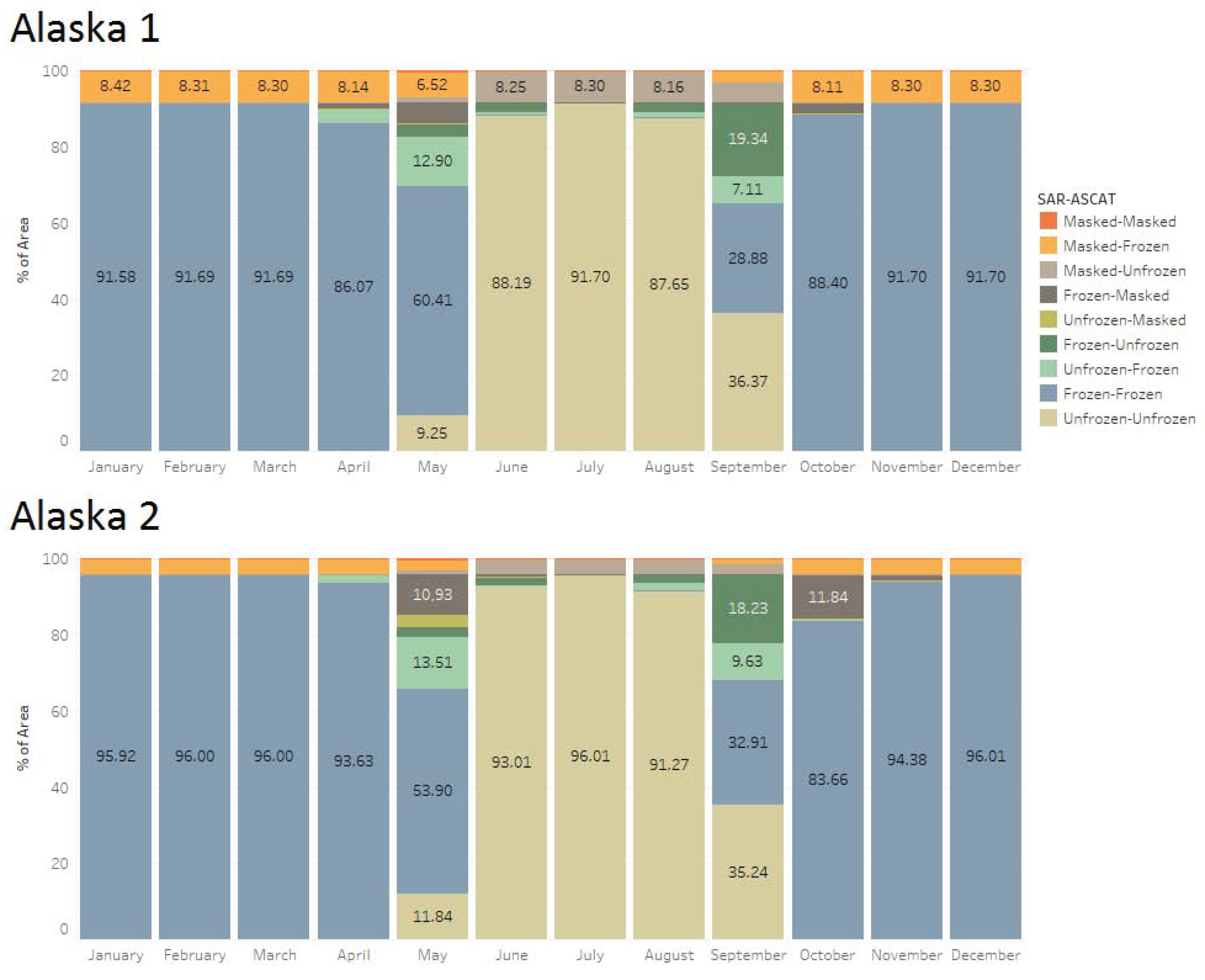
Figure 2 shows an example of the temporal differences of freeze/thaw products for the selected ASCAT grid cells in Alaska, averaged for 2007–2010. The discrepancies are mainly limited to May and September (with small differences in April, June, July, August and October), emphasizing the importance of transitional periods. The visible differences in the remaining months (up to 8.4% in the case of Alaska 1) are limited to areas masked within the SAR product. More than 50% of the area (accumulated for all days) remains frozen in May in SAR, as well as ASCAT in the shown examples. The switch for ASCAT occurs in September with only approximately 30% of agreement with SAR. Almost 20% of the landscape already freezes before the switch in ASCAT.
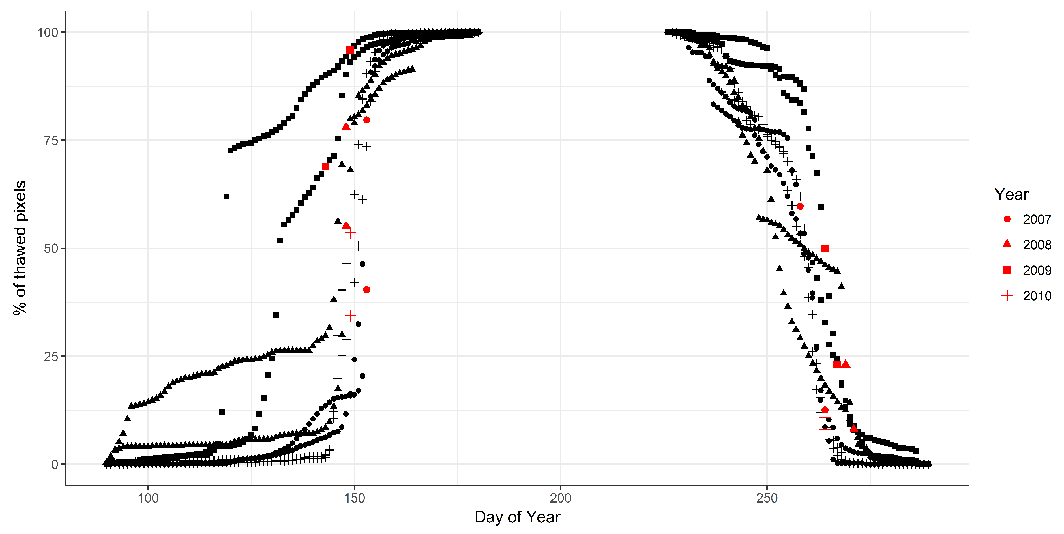
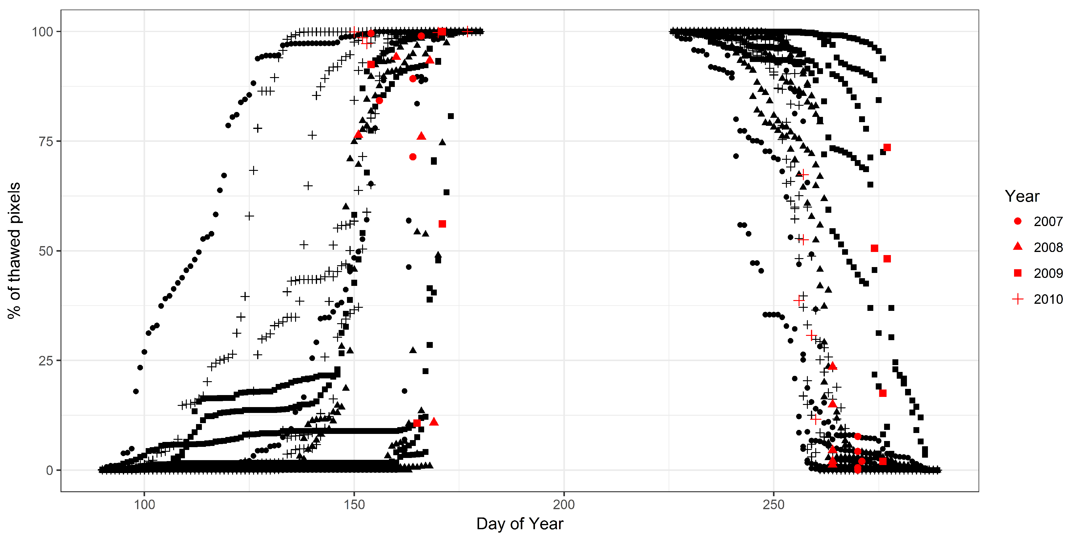
Figure 8, Figure 9, Figure 10 and Figure 11 show the actual time series of thawed SAR pixels within one ASCAT grid cell for the situation in spring and autumn as indicated by the day of the year. The results confirm differences between spring and autumn, but differences between the analyzed years, as well. Figure 8 shows the results for the two selected ASCAT grid cells in Alaska (as in Figure 2). Both grid cells have a high variability in the SAR data between the observed years for spring compared to autumn. Especially the onset of the thawing process is more variable than the onset of the freezing process. These characteristics can also be found in most, but not all, of the other selected ASCAT grid cells (Figure 9, Figure 10 and Figure 11).
An example of a more detailed view of the progress of thawing SAR pixel within one ASCAT grid cell is shown in Figure 12. The shape of the curve is different in all of the studied years and cannot be described adequately with a linear regression. R2 ranges from 0.75–0.89, but the slope and intercept varies from year to year. The shape is sigmoid, suggesting a better fit with a logistic function.
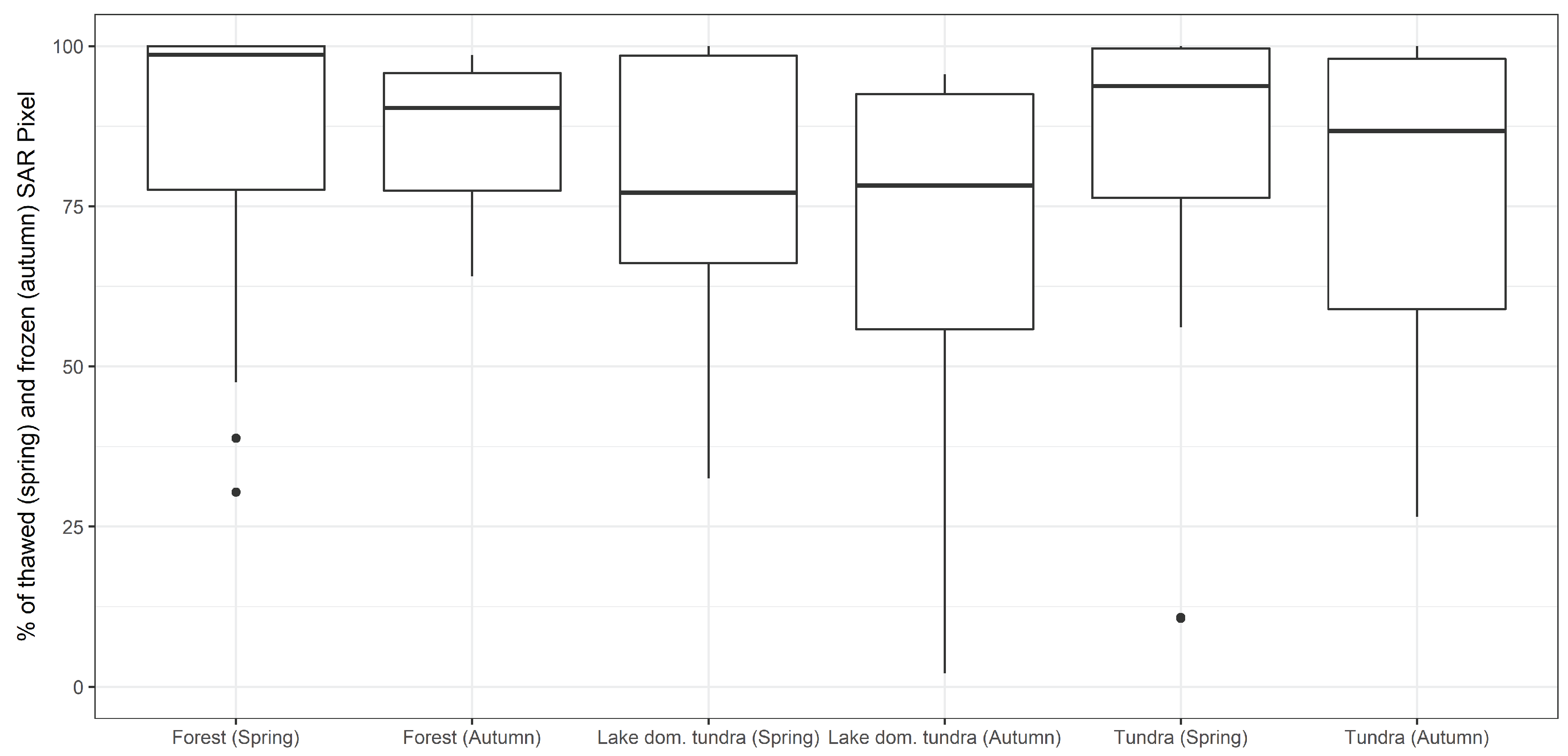
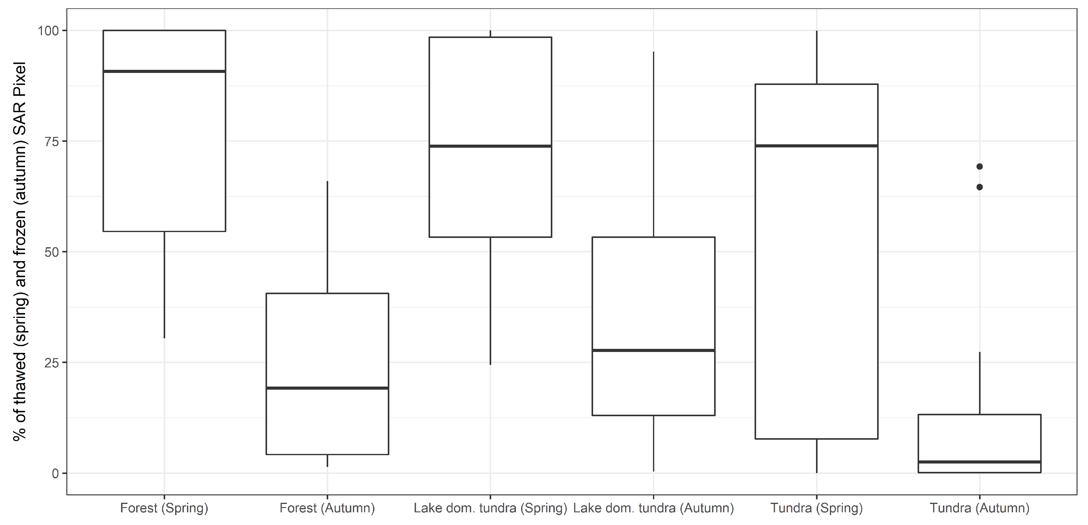
During the beginning of the transitional period, the surface state as reported by the ASCAT dataset can change from frozen to thawed and back in spring (from thawed to frozen and back in autumn) several times due to day to day fluctuations in the air temperature. The percentage of thawed/frozen SAR pixels within the ASCAT grid cell at the timing of the last surface state change reported by the ASCAT product varies greatly; not only between the different grid cells, but also for each of the sites individually, in spring, as well as in autumn. The percentage of already thawed or frozen SAR cells within one ASCAT grid cell, as well as the variability of this parameter varies between landscape types. Figure 13 shows the median, minimum and maximum of the percentages of frozen and thawed SAR pixels for autumn and spring, respectively visualized as box plots. During freeze-up, lake-rich pixels show the largest variability, while all values for forest lie above 60%. Pixels dominated by tundra and lake-rich environments both show a smaller variability during thawing compared to freeze-up. For pixels dominated by forest environments, this is reversed: the percentages of frozen SAR cells are more variable for thawing conditions than freezing. The percentage of thawed/frozen SAR pixels within one ASCAT footprint at the timing of the first surface state change shows a larger variability as illustrated by Figure 14. All landscape types show a high variability of percentages for both spring and autumn, except for landscape type tundra, which shows low variability in autumn.
A comparison of the median number of SAR acquisitions in each year with the median of discrepancy days for each grid cell revealed no clear relationship between the two parameters (see Figure 15). The number of available acquisitions in the SAR archives differs between North America and Eastern Siberia. It is in general less than 100 or more than 200, respectively. The median is in both cases usually in the order of two weeks and can be more than a month in both cases.
A difference between freezing and thawing periods can be also observed in the spatial patterns. They differ considerably between the selected landscape types for spring and autumn. While some grid cells have no clear patterns, others show distinct differences for spring and autumn. An overview of all selected grid cells, including the standard deviation of discrepancies between the two freeze/thaw products, is summarized in Table 1. The standard deviation of discrepancy values in spring is higher compared to autumn for most investigated grid cells. This is supported by the patterns seen in Figure 16, which shows scatterplots of the four-year mean values of discrepancy days for the selected grid cells. While most grid cells show a higher standard deviation in spring compared to autumn, the variability between the two seasons is differently pronounced (see Table 1). Grid cells that are dominated by lakes (see Table 1) show higher values of the standard deviation in autumn compared to tundra-dominated sites (except Laptev Sea 5 ()). Within landscape types, tundra shows the most differences with standard deviations in autumn ranging from 7.58 (Laptev Sea 2) to 22.66 (Laptev Sea 5). Laptev Sea 5 shows the lowest elevation of all tundra grid cells; Table 1.
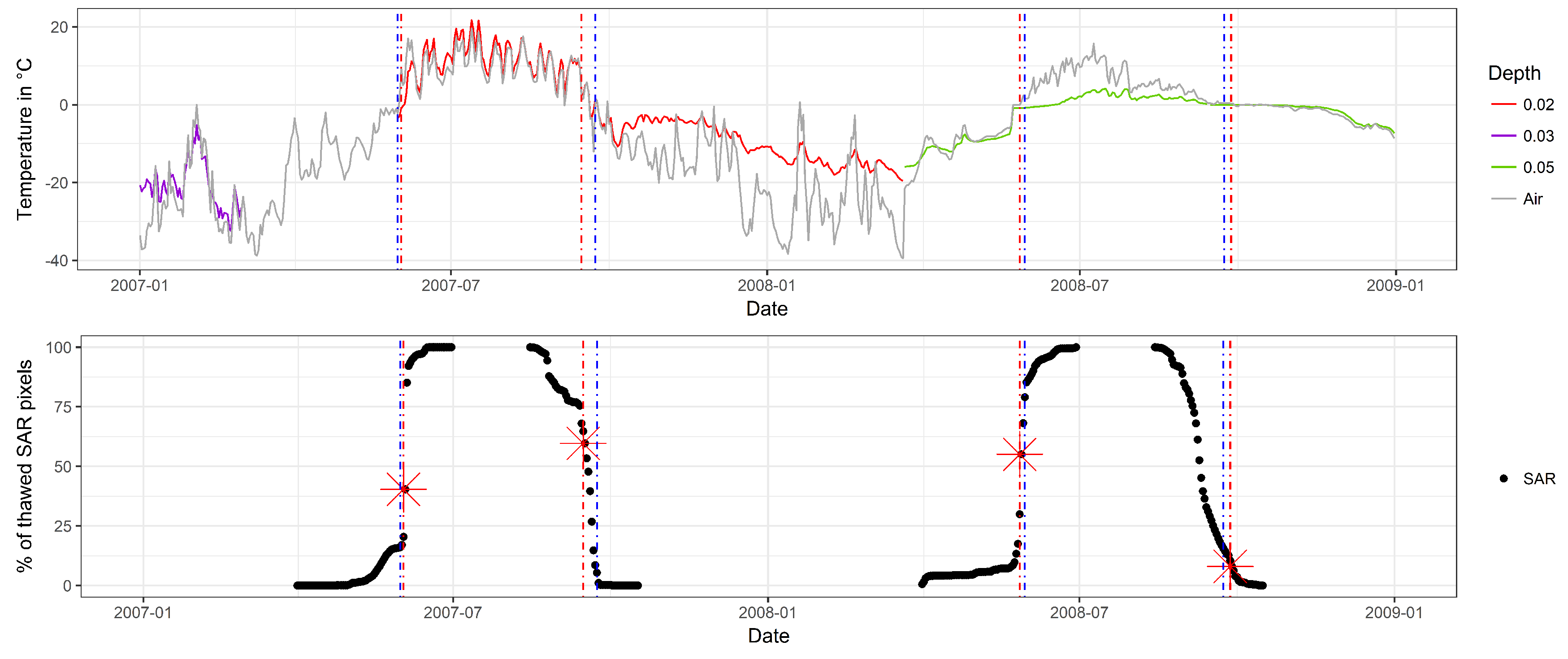
The comparison of ASCAT and SAR data with in situ temperature measurements for the grid cell Alaska 2 for two years is shown in Figure 17. The difference can be negative, as well as positive in both spring and autumn, e.g., ASCAT freeze-up in 2007 occurs when when temperatures drop to almost zero at the measurements site, but SAR shows a later switch when below zero temperature values are reached locally. This differs in 2008 where the freeze-transition is smoother than in 2007. The unfrozen day in spring occurs in all cases after a period with temperatures close to zero. In the case of soil temperatures (as available in 2008), this period can be interpreted as a melting snow situation [19]. Freeze-up occurs comparably late at the Sagwon site in both years. With an altitude of 278 m, it is located higher than the average elevation in this grid cell.
4. Discussion
4.1. Spatial Patterns
The observed spatial discrepancies between freeze/thaw data from the two datasets [41] and [42] show distinct regional differences. The lake mask, included in the SAR product, causes pronounced differences between the SAR and the ASCAT datasets. This is visible in the regional results, which show a high number of discrepancy days in the regions of the Mackenzie Delta and the Lena River Delta (see Figure 4 and Figure 5). The backscatter over lakes drops after melt and does not increase afterwards as for the surrounding land area. Wind action over the lakes can increase the average backscatter within the ASCAT footprint on a short-term basis [21], which may lead to misclassifications. The regional results also show linear artifacts, which are caused by SAR processing issues with the NEST software [41].
Snow and snow melt are known to influence the freeze/thaw detectability [57] of coarse resolution products. The variability in the onset of snow melt leads to a spatial heterogeneity in the timing of the following freeze/thaw transition on a small scale [1], which can potentially be picked up by the 1-km resolution of the SAR product, but is overlooked by the ASCAT sensor, leading to high spatial variability in discrepancies during the spring transition on a grid cell level.
Discrepancies for grid cells in tundra regions can be partially attributed to uncertainties in the lake mask used to create the SAR product, lakes not covered by the lake mask due to their small size and the fact that lakes are not masked in the ASCAT product and therefore influence the resulting values. Additionally, lake-rich landscapes exhibit heterogeneity in soil moisture [58], which influences the freeze-back process, as well as the intensity of the backscatter response [27]. These areas therefore partially exhibit a freezing pattern not representative of the overall ASCAT cell extent. To analyze spatial patterns in greater detail, especially in heterogeneous landscapes, freeze/thaw products based on enhanced resolution scatterometer data (e.g., [45]) would be beneficial, but are not yet available.
The comparison of discrepancy days in spring and autumn as shown in Figure 16 reveals distinct groupings of pixels showing large discrepancies in both spring and autumn and smaller groupings of pixels with low discrepancy values for both seasons.
4.2. Temporal Patterns
The temporal analysis of discrepancies in freeze/thaw data focused on the transitional periods, as this is the only time the datasets were inconsistent with the exception of masked areas. The difference in surface state information of the two data products is dependent on the day of the year and with that the advance of the freezing and thawing progress. The percentage of already thawed or frozen SAR pixel at the time of the surface state change in the ASCAT product varies between the analyzed years, as well as between the selected study sites. These variations occur in both spring and autumn. This is also demonstrated in Figure 17. The increase in percentage of frozen and thawed SAR pixel per ASCAT grid cell is a non-linear process, especially in the beginning of the freezing and thawing of the grid cell. This, together with the different percentages of frozen and thawed pixels at the time of the ASCAT surface state change would impact future attempts to downscale spatially coarse freeze/thaw products. The SAR product used in this analysis gives no information about temporal dynamics, as it only includes a single DOY for freezing and thawing, respectively. The ASCAT product shows the temporal dynamics of the freezing and thawing process; multiple changes of the surface state happen during every transitional period covered by this dataset. Only the last change in spring and autumn respectively is considered for this study. Due to this difference, the two datasets naturally disagree on temporal dynamics.
Additionally, the difference in the acquisition times of ASCAT and ASAR data is thought to influence the results. ASCAT, as well as SAR datasets include afternoon acquisitions for Alaska and Mackenzie. For Siberia, data from ascending orbits are acquired earlier for both SAR and ASCAT. Diurnal freeze/thaw cycles of the snow surface [23] and subsequently the ground surface occur during transitional periods [59]. Consequently, a comparison of freeze/thaw values retrieved at different (local) times might not be appropriate during spring and autumn when the surface state can be highly dynamic [23,60]. However, a detailed analysis of the influence on the spatial patterns cannot be made, as the number of SAR acquisitions differs considerable between the sites and data from both orbits, and thus, different timings have been used in the case of both SAR and ASCAT products.
The comparison of in situ measurements with the results for grid cell Alaska 2 revealed a good agreement between the timing of ASCAT and SAR surface state, as well as with air and near-surface soil temperature. A more comprehensive comparison of the results with additional in situ measurements would be beneficial for possible downscaling attempts, but is limited by data availability. None of the other selected grid cells (complying with the strict criteria of data availability, etc.) contained measurement sites with openly accessible data. An alternative might be reanalyses data, but they have only coarse spatial resolution of about 80 km [61].
In this study, we considered the timing of thaw as the conditions after snow melt. While the ASCAT product gives information about melting snow [20], we did not consider this in our analysis as the ASAR product contains no such information [35]. As discussed above, temporal dynamics of discrepancies have been found to be variable between years and study sites. A similar analysis focusing on the start of snow melt might produce different results. The start and duration of snow melt is highly variable across the Arctic [62] as derived from QuikScat, which provides high temporal resolution that allows one to consider diurnal effects, which are of relevance in the case of snow melt detection [23]. A sensor with higher acquisition intervals than ASCAT over the Arctic land area would be required. The issue is even more problematic in the case of SAR acquisitions.
4.3. Importance of Landscape Types on the Issue of Scale
The landscape types show distinct differences in their variability of the share of thawed or frozen SAR pixels at the time of the last change in the ASCAT dataset. While tundra and lake-rich landscapes show a smaller variability in spring, forest landscapes show a smaller variability in autumn. The high variability of forest landscapes in spring could be attributed to snow melt, which is a heterogeneous process in forest-dominated landscapes [63]. Park et al. [35] found different relationships for the spring transition date and the timing of snow melt for tundra and forest environments. While the spring transition date for tundra landscapes corresponded to the end of the snow melt, it was correlated with the beginning of the snow melt period in forest landscapes [35]. The variability of the percentages of thawed or frozen SAR pixels at the time of the first surface state change as reported in the ASCAT product shows a larger variability. While the variability is high for both autumn and spring, all landscape types show a lower median in autumn. The difference between the landscape types is not as distinct as the difference between the two seasons. This could partially be due to the influence of snow cover in spring, which influences the thaw timing. This would also account for the different variability of the results for timing of the first and the last surface state change as reported in the ASCAT product. Snow melt or still present snow cover within the ASCAT footprint would have more influence on the results during the time of the first surface state change. The accuracy of the SAR data product is generally believed to be higher during freeze-up compared to thaw [41], leading to a more reliable detection of early frozen SAR pixel within one ASCAT grid cell. A higher accuracy in detecting early freeze-up in the SAR product could therefore account for the lower medians in autumn for the time of the first surface state change.
The high variability of lake-rich landscapes could be attributed to the influence of lake ice break-up and formation, which is known to influence backscatter at C-band [64], as well as the presence of remaining open water in autumn. Floating ice produces relatively high backscatter (higher compared to summer values) [49]; therefore, the presence of lakes reduces backscatter in summer, under calm conditions, increases short term under windy conditions [65], and floating ice remains after snow melt [66] and increases backscatter in winter (depending on ice growth patterns). This all introduces noise that may lead to a lower performance of the threshold and edge detection algorithms. While being mainly masked out in the SAR product, lakes potentially influence the ASCAT backscatter signal and with this the accuracy of the ASCAT freeze/thaw detection capability. While it is clear that the ASCAT product is influenced by sub-pixel lakes, the SAR information might also be partially affected due to uncertainties in the lake mask and the abundance of ponds much smaller than can be captured with the 1-km resolution [67].
4.4. Influence of Data Quality
The importance of the number of acquisitions considered in the SAR freeze/thaw product is visible in the regional results when comparing results for the Ob Estuary region (E) with the corresponding SAR coverage (see Figure 3 and Figure 5). However, when comparing the median number of discrepancy days with the median number of considered SAR acquisitions for the selected grid cells, no relationship between the two parameters can be detected (see Figure 15). This suggests the importance of adequate SAR coverage up to a certain threshold, but also points towards a robustness of the surface state retrieval algorithm once the threshold of the minimum number of acquisitions as selected by Park et al. [35] is reached. As the ASCAT grid cells were specifically chosen to have similar coverage numbers each year, the results do not allow conclusions about site-specific relationships of discrepancies and coverage.
Acquisition timing may play a role for detection accuracy with both approaches, the location-based threshold, as well as the step function method. Both freely-available products mix ascending and descending orbit data for higher temporal sampling. Further investigations are required to investigate this issue.
5. Conclusions
The analyses in this paper provide a first step in developing a downscaling scheme for coarse resolution C-band scatterometer-based land surface freeze/thaw information. The importance of land cover, especially forests and lakes, is confirmed and its impact quantified. Differences between the two data products in both spring and autumn were found for all sites; the intensity of the observed discrepancies varied considerably between the studied grid cells. Results for different landscape types showed distinctly different standard deviations in spring and autumn, with lake-dominated landscapes showing comparatively high standard deviations in autumn. Forest-dominated grid cells are especially variable in spring due to the influences of a delayed snow melt process. The differences are smallest for tundra sites without water bodies for both thaw and freeze-up, with highest agreement in autumn. Compared to L-band, frequent C-band SAR observations are freely available for the past and will increase in the future with the Sentinel-1 mission. The latter will even allow 10–30-m spatial resolution analyses. A further advantage of C-band is the current developments in the resolution enhancement of ASCAT data.
Results from this analysis underline the importance of landscape-specific approaches when dealing with active microwave remote sensing data at different spatial and temporal resolutions. Especially in down- or up-scaling approaches, this becomes of major importance. Besides highlighting, the discrepancies between the scales, this study also shows the findings of the spatial heterogeneity of the thaw and freeze-up process for different permafrost landscapes. The identified differences between forest and tundra landscape match previous findings by Park et al. [35]. We found the progress of thaw and freeze-up within an ASCAT grid cell to be specific to study site and year. Preliminary tests showed that the progression is best described by a logistic function.
Acknowledgments
This work was supported by the Austrian Science Fund (Fonds zur Förderung der wissenschaftlichen Forschung, FWF) through the Doctoral College GIScience (DK W1237-N23). We would like to thank the four anonymous reviewers for their valuable comments.
Author Contributions
Helena Bergstedt conducted all data processing and analysis, the literature research, designed the figures and wrote the majority of the manuscript. Annett Bartsch contributed to the concept for this study, as well as to the interpretation of the results and to the writing of the manuscript.
Conflicts of Interest
The authors declare no conflict of interest. The founding sponsors had no role in the design of the study; in the collection, analyses or interpretation of data; in the writing of the manuscript; nor in the decision to publish the results.
References
- Kimball, J.; McDonald, K.; Frolking, S.; Running, S. Radar remote sensing of the spring thaw transition across a boreal landscape. Remote Sens. Environ. 2004, 89, 163–175. [Google Scholar] [CrossRef]
- Yi, Y.; Kimball, J.S.; Jones, L.A.; Reichle, R.H.; Nemani, R.; Margolis, H.A. Recent climate and fire disturbance impacts on boreal and arctic ecosystem productivity estimated using a satellite-based terrestrial carbon flux model. J. Geophys. Res. Biogeosci. 2013, 118, 606–622. [Google Scholar] [CrossRef]
- Wang, G.; Hu, H.; Li, T. The influence of freeze-thaw cycles of active soil layer on surface runoff in a permafrost watershed. J. Hydrol. 2009, 375, 438–449. [Google Scholar] [CrossRef]
- Qi, J.; Vermeer, P.A.; Cheng, G. A review of the influence of freeze-thaw cycles on soil geotechnical properties. Permafr. Periglac. Process. 2006, 17, 245–252. [Google Scholar] [CrossRef]
- Manasypov, R.M.; Vorobyev, S.N.; Loiko, S.V.; Kritzkov, I.V.; Shirokova, L.S.; Shevchenko, V.P.; Kirpotin, S.N.; Kulizhsky, S.P.; Kolesnichenko, L.G.; Zemtzov, V.A.; et al. Seasonal dynamics of organic carbon and metals in thermokarst lakes from the discontinuous permafrost zone of western Siberia. Biogeosciences 2015, 12, 3009–3028. [Google Scholar] [CrossRef]
- Gruber, S.; Hoelzle, M.; Haeberli, W. Permafrost thaw and destabilization of Alpine rock walls in the hot summer of 2003. Geophys. Res. Lett. 2004, 31, L13504. [Google Scholar] [CrossRef]
- Mastepanov, M.; Sigsgaard, C.; Dlugokencky, E. Large tundra methane burst during onset of freezing. Nature 2008, 456, 628–630. [Google Scholar] [CrossRef] [PubMed]
- Zhang, T.; Barry, R.G.; Armstrong, R.L. Application of Satellite Remote Sensing Techniques to Frozen Ground Studies. Polar Geogr. 2004, 28, 163–196. [Google Scholar] [CrossRef]
- Raynolds, M.K.; Walker, D.A.; Ambrosius, K.J.; Brown, J.; Everett, K.R.; Kanevskiy, M.; Kofinas, G.P.; Romanovsky, V.E.; Shur, Y.; Webber, P.J. Cumulative geoecological effects of 62 years of infrastructure and climate change in ice-rich permafrost landscapes, Prudhoe Bay Oilfield, Alaska. Glob. Chang. Biol. 2014, 20, 1211–1224. [Google Scholar] [CrossRef] [PubMed]
- Schaefer, K.; Zhang, T.; Bruhwiler, L.; Barrett, A.P. Amount and timing of permafrost carbon release in response to climate warming. Tellus Ser. B 2011, 63, 165–180. [Google Scholar] [CrossRef]
- Spencer, R.G.M.; Mann, P.J.; Dittmar, T.; Eglinton, T.I.; McIntyre, C.; Holmes, R.M.; Zimov, N.; Stubbins, A. Detecting the signature of permafrost thaw in Arctic rivers. Geophys. Res. Lett. 2015, 42, 2830–2835. [Google Scholar] [CrossRef]
- Grosse, G.; Goetz, S.; McGuire, A.D.; Romanovsky, V.E.; Schuur, E.A.G. Changing permafrost in a warming world and feedbacks to the Earth system. Environ. Res. Lett. 2016, 11, 040201. [Google Scholar] [CrossRef]
- Vincent, W.F.; Lemay, M.; Allard, M. Arctic permafrost landscapes in transition: Towards an integrated Earth system approach. Arct. Sci. 2017, 3, 39–64. [Google Scholar] [CrossRef]
- Podest, E.; McDonald, K.C.; Kimball, J.S. Multisensor Microwave Sensitivity to Freeze/Thaw Dynamics Across a Complex Boreal Landscape. IEEE Trans. Geosci. Remote Sens. 2014, 52, 6818–6828. [Google Scholar] [CrossRef]
- Wegmüller, U. The effect of freezing and thawing on the microwave signatures of bare soil. Remote Sens. Environ. 1990, 33, 123–135. [Google Scholar] [CrossRef]
- Kimball, J.; McDonald, K.; Keyser, A.; Frolking, S.; Running, S. Application of the NASA Scatterometer (NSCAT) for Determining the Daily Frozen and Nonfrozen Landscape of Alaska. Remote Sens. Environ. 2001, 75, 113–126. [Google Scholar] [CrossRef]
- Rautiainen, K.; Parkkinen, T.; Lemmetyinen, J.; Schwank, M.; Wiesmann, A.; Ikonen, J.; Derksen, C.; Davydov, S.; Davydova, A.; Boike, J.; et al. SMOS prototype algorithm for detecting autumn soil freezing. Remote Sens. Environ. 2016, 180, 346–360. [Google Scholar] [CrossRef]
- Xu, X.; Derksen, C.; Yueh, S.H.; Dunbar, R.S.; Colliander, A. Freeze/Thaw Detection and Validation Using Aquarius’ L-Band Backscattering Data. IEEE J. Sel. Top. Appl. Earth Obs. Remote Sens. 2016, 9, 1370–1381. [Google Scholar] [CrossRef]
- Zwieback, S.; Paulik, C.; Wagner, W. Frozen Soil Detection Based on Advanced Scatterometer Observ. and Air Temperature Data as Part of Soil Moisture Retrieval. Remote Sens. 2015, 7, 3206–3231. [Google Scholar] [CrossRef]
- Naeimi, V.; Paulik, C.; Bartsch, A.; Wagner, W.; Kidd, R.; Park, S.E.; Elger, K.; Bioke, J. ASCAT Surface State Flag (SSF): Extracting Information on Surface Freeze/Thaw Conditions From Backscatter Data Using an Empirical Threshold-Analysis Algorithm. IEEE Trans. Geosci. Remote Sens. 2012, 50, 2566–2582. [Google Scholar] [CrossRef]
- Högström, E.; Trofaier, A.M.; Gouttevin, I.; Bartsch, A. Assessing Seasonal Backscatter Variations with Respect to Uncertainties in Soil Moisture Retrieval in Siberian Tundra Regions. Remote Sens. 2014, 6, 8718–8738. [Google Scholar] [CrossRef]
- Boehnke, K.; Wismann, V.R. Thawing of soils in Siberia observed by the ERS-1 scatterometer between 1992 and 1995. In Proceedings of the International Geoscience and Remote Sensing Symposium, IGARSS ’96—Remote Sensing for a Sustainable Future, Lincoln, NE, USA, 31 May 1996; Volume 4, pp. 2264–2266. [Google Scholar]
- Bartsch, A.; Kidd, R.A.; Wagner, W.; Bartalis, Z. Temporal and spatial variability of the beginning and end of daily spring freeze/thaw cycles derived from scatterometer data. Remote Sens. Environ. 2007, 106, 360–374. [Google Scholar] [CrossRef]
- Bartsch, A.; Kumpula, T.; Forbes, B.C.; Stammler, F. Detection of snow surface thawing and refreezing in the Eurasian Arctic with QuikSCAT: Implications for reindeer herding. Ecol. Appl. 2010, 20, 2346–2358. [Google Scholar] [CrossRef] [PubMed]
- Foster, J.L.; Hall, D.K.; Eylander, J.B.; Riggs, G.A.; Nghiem, S.V.; Tedesco, M.; Kim, E.; Montesano, P.M.; Kelly, R.E.J.; Casey, K.A.; et al. A blended global snow product using visible, passive microwave and scatterometer satellite data. Int. J. Remote Sens. 2011, 32, 1371–1395. [Google Scholar] [CrossRef]
- Wang, L.; Derksen, C.; Brown, R. Detection of pan-Arctic terrestrial snowmelt from QuikSCAT, 2000–2005. Remote Sens. Environ. 2008, 112, 3794–3805. [Google Scholar] [CrossRef]
- Widhalm, B.; Bartsch, A.; Heim, B. A Novel Approach for the Characterization of Tundra Wetland Regions with C-band SAR Satellite Data. Int. J. Remote Sens. 2015, 36, 5537–5556. [Google Scholar] [CrossRef] [PubMed] [Green Version]
- Brown, R.; Derksen, C.; Wang, L. Assessment of spring snow cover duration variability over northern Canada from satellite datasets. Remote Sens. Environ. 2007, 111, 367–381. [Google Scholar] [CrossRef]
- Zwieback, S.; Bartsch, A.; Melzer, T.; Wagner, W. Probabilistic Fusion of Ku—And C-band Scatterometer Data for Determining the Freeze/Thaw State. IEEE Trans. Geosci. Remote Sens. 2012, 50, 2583–2594. [Google Scholar] [CrossRef]
- Drobot, S.D.; Anderson, M.R. An improved method for determining snowmelt onset dates over Arctic sea ice using scanning multichannel microwave radiometer and Special Sensor Microwave/Imager data. J. Geophys. Res. Atmos. 2001, 106, 24033–24049. [Google Scholar] [CrossRef]
- Winebrenner, D.P.; Nelson, E.D.; Colony, R.; West, R.D. Observation of melt onset on multiyear Arctic sea ice using the ERS 1 synthetic aperture radar. J. Geophys. Res. Oceans 1994, 99, 22425–22441. [Google Scholar] [CrossRef]
- Mortin, J.; Howell, S.E.; Wang, L.; Derksen, C.; Svensson, G.; Graversen, R.G.; Schrøder, T.M. Extending the QuikSCAT record of seasonal melt–freeze transitions over Arctic sea ice using ASCAT. Remote Sens. Environ. 2014, 141, 214–230. [Google Scholar] [CrossRef]
- Howell, S.E.; Derksen, C.; Tivy, A. Development of a water clear of sea ice detection algorithm from enhanced SeaWinds/QuikSCAT and AMSR-E measurements. Remote Sens. Environ. 2010, 114, 2594–2609. [Google Scholar] [CrossRef]
- Derksen, C.; Xu, X.; Dunbar, R.S.; Colliander, A.; Kim, Y.; Kimball, J.S.; Black, T.A.; Euskirchen, E.; Langlois, A.; Loranty, M.M.; et al. Retrieving landscape freeze/thaw state from Soil Moisture Active Passive (SMAP) radar and radiometer measurements. Remote Sens. Environ. 2017, 194, 48–62. [Google Scholar] [CrossRef]
- Park, S.E.; Bartsch, A.; Sabel, D.; Wagner, W.; Naeimi, V.; Yamaguchi, Y. Monitoring freeze/thaw cycles using ENVISAT ASAR Global Mode. Remote Sens. Environ. 2011, 115, 3457–3467. [Google Scholar] [CrossRef]
- Park, H.; Kim, Y.; Kimball, J.S. Widespread permafrost vulnerability and soil active layer increases over the high northern latitudes inferred from satellite remote sensing and process model assessments. Remote Sens. Environ. 2016, 175, 349–358. [Google Scholar] [CrossRef]
- Roy, A.; Toose, P.; Williamson, M.; Rowlandson, T.; Derksen, C.; Royer, A.; Berg, A.A.; Lemmetyinen, J.; Arnold, L. Response of L-Band brightness temperatures to freeze/thaw and snow dynamics in a prairie environment from ground-based radiometer measurements. Remote Sens. Environ. 2017, 191, 67–80. [Google Scholar] [CrossRef]
- Rautiainen, K.; Lemmetyinen, J.; Schwank, M.; Kontu, A.; Ménard, C.B.; Mätzler, C.; Drusch, M.; Wiesmann, A.; Ikonen, J.; Pulliainen, J. Detection of soil freezing from L-band passive microwave observations. Remote Sens. Environ. 2014, 147, 206–218. [Google Scholar] [CrossRef]
- Rignot, E.; Way, J.B. Monitoring Freeze-Thaw Cycles along North-South Alaskan Transects Using ERS-1 SAR. Remote Sens. Environ. 1994, 49, 131–137. [Google Scholar] [CrossRef]
- Way, J.B.; Zimmermann, R.; Rignot, E.; McDonald, K.; Oren, R. Winter and spring thaw as observed with imaging radar at BOREAS. J. Geophys. Res. Atmos. 1997, 102, 29673–29684. [Google Scholar] [CrossRef]
- Sabel, D.; Park, S.E.; Bartsch, A.; Schlaffer, S.; Klein, J.P.; Wagner, W. Regional Surface Soil Moisture and Freeze/Thaw Timing Remote Sensing Products with Links to Geotiff Images. 2012. Available online: https://doi.pangaea.de/10.1594/PANGAEA.779658 (accessed on 20 November 2015).
- Paulik, C.; Melzer, T.; Hahn, S.; Bartsch, A.; Heim, B.; Elger, K.; Wagner, W. Circumpolar Surface Soil Moisture and Freeze/Thaw Surface Status Remote Sensing Products (Version 4) with Links to Geotiff Images and NetCDF Files (2007-01 to 2013-12). 2014. Available online: https://doi.pangaea.de/10.1594/PANGAEA.832153 (accessed on 20 November 2015).
- Roy, A.; Royer, A.; Derksen, C.; Brucker, L.; Langlois, A.; Mialon, A.; Kerr, Y.H. Evaluation of Spaceborne L-Band Radiometer Measurements for Terrestrial Freeze/Thaw Retrievals in Canada. IEEE J. Sel. Top. Appl. Earth Obs. Remote Sens. 2015, 8, 4442–4459. [Google Scholar] [CrossRef]
- Entekhabi, D.; Njoku, E.G.; O’Neill, P.E.; Kellogg, K.H.; Crow, W.T.; Edelstein, W.N.; Entin, J.K.; Goodman, S.D.; Jackson, T.J.; Johnson, J.; et al. The Soil Moisture Active Passive (SMAP) Mission. Proc. IEEE 2010, 98, 704–716. [Google Scholar] [CrossRef]
- Lindsley, R.D.; Long, D.G. Enhanced-Resolution Reconstruction of ASCAT Backscatter Measurements. IEEE Trans. Geosci. Remote Sens. 2016, 54, 2589–2601. [Google Scholar] [CrossRef]
- Bartsch, A.; Seifert, F.M. The ESA DUE Permafrost project—A service for high latitude research. In Proceedings of the 2012 IEEE International Geoscience and Remote Sensing Symposium (IGARSS), Munich, Germany, 22–27 July 2012; pp. 5222–5225. [Google Scholar]
- Rodell, M.; Houser, P.R.; Jambor, U.E.A.; Gottschalck, J.; Mitchell, K.; Meng, C.J.; Arsenault, K.; Cosgrove, B.; Radakovich, J.; Bosilovich, M. The global land data assimilation system. Bull. Am. Meteorol. Soc. 2004, 85, 381–394. [Google Scholar] [CrossRef]
- Dee, D.P.; Uppala, S.M.; Simmons, A.J.; Berrisford, P.; Poli, P.; Kobayashi, S.; Andrae, U.; Balmaseda, M.A.; Balsamo, G.; Bauer, P.; et al. The ERA-Interim reanalysis: Configuration and performance of the data assimilation system. Q. J. R. Meteorol. Soc. 2011, 137, 553–597. [Google Scholar] [CrossRef]
- Bartsch, A.; Pointner, G.; Leibman, M.O.; Dvornikov, Y.A.; Khomutov, A.V.; Trofaier, A.M. Circumpolar Mapping of Ground-Fast Lake Ice. Front. Earth Sci. 2017, 5, 12. [Google Scholar] [CrossRef]
- Pathe, C.; Wagner, W.; Sabel, D.; Doubkova, M.; Basara, J.B. Using ENVISAT ASAR Global Mode Data for Surface Soil Moisture Retrieval Over Oklahoma, USA. IEEE Trans. Geosci. Remote Sens. 2009, 47, 468–480. [Google Scholar] [CrossRef]
- Latifovic, R.; Zhu, Z.; Cihlar, J.; Beaubien, J.; Fraser, R. The Land Cover Map for North America in the Year 2000, GLC2000 Database; European Commision Joint Research Centre: Brussels, Belgium, 2003; Available online: http://www-gem.jrc.it/glc2000 (accessed on 20 February 2017).
- Belward, A.S.; Erchov, D.V.; Isaev, A.S.; Bartholom, E.; Gond, V.; Vogt, P.; Achard, F.; Zubkov, A.M.; Mollicone, D.; Savin, I.; et al. The Land Cover Map for Northern Eurasia for the Year 2000, GLC2000 Database; European Commision Joint Research Centre: Brussels, Belgium, 2003; Available online: http://www-gem.jrc.it/glc2000 (accessed on 20 February 2017).
- Brown, O.; Heginbottom, J.; Melnikov, E. Circum-Arctic Map of Permafrost and Ground-Ice Conditions, 2nd ed.; National Snow and Ice Data Center: Boulder, CO, USA, 2002. [Google Scholar]
- Kane, D.; Hinzman, L. Climate Data from the North Slope Hydrology Research Project. University of Alaska Fairbanks, Water and Environmental Research Center, 2017. Available online: http://ine.uaf.edu/werc/projects/NorthSlope/ (accessed on 2 July 2017).
- GTN-P. Global Terrestrial Network for Permafrost Database: Permafrost Temperature Data (TSP—Thermal State of Permafrost); International Permafrost Association: Akureyri, Iceland, 2016. [Google Scholar]
- Santoro, M.; Strozzi, T. Circumpolar Digital Elevation Models > 55° N with Links to Geotiff Images. 2012. Available online: https://doi.pangaea.de/10.1594/PANGAEA.779748 (accessed on 20 April 2017).
- Reschke, J.; Bartsch, A.; Schlaffer, S.; Schepaschenko, D. Capability of C-Band SAR for Operational Wetland Monitoring at High Latitudes. Remote Sens. 2012, 4, 2923–2943. [Google Scholar] [CrossRef] [Green Version]
- Sturtevant, C.S.; Oechel, W.C. Spatial variation in landscape-level CO2 and CH4 fluxes from arctic coastal tundra: Influence from vegetation, wetness, and the thaw lake cycle. Glob. Chang. Biol. 2013, 19, 2853–2866. [Google Scholar] [CrossRef] [PubMed]
- Hinkel, K.; Paetzold, F.; Nelson, F.; Bockheim, J. Patterns of soil temperature and moisture in the active layer and upper permafrost at Barrow, Alaska: 1993–1999. Glob. Planet. Chang. 2001, 29, 293–309. [Google Scholar] [CrossRef]
- Han, L.; Tsunekawa, A.; Tsubo, M. Monitoring near-surface soil freeze–thaw cycles in northern China and Mongolia from 1998 to 2007. Int. J. Appl. Earth Obs. Geoinf. 2010, 12, 375–384. [Google Scholar] [CrossRef]
- Balsamo, G.; Albergel, C.; Beljaars, A.; Boussetta, S.; Brun, E.; Cloke, H.; Dee, D.; Dutra, E.; Muñoz Sabater, J.; Pappenberger, F.; et al. ERA-Interim/Land: A global land surface reanalysis dataset. Hydrol. Earth Syst. Sci. 2015, 19, 389–407. [Google Scholar] [CrossRef]
- Bartsch, A. Ten Years of SeaWinds on QuikSCAT for Snow Applications. Remote Sens. 2010, 2, 1142–1156. [Google Scholar] [CrossRef]
- Davis, R.E.; Hardy, J.P.; Ni, W.; Woodcock, C.; McKenzie, J.C.; Jordan, R.; Li, X. Variation of snow cover ablation in the boreal forest: A sensitivity study on the effects of conifer canopy. J. Geophys. Res. Atmos. 1997, 102, 29389–29395. [Google Scholar] [CrossRef]
- Du, J.; Kimball, J.S.; Duguay, C.; Kim, Y.; Watts, J.D. Satellite microwave assessment of Northern Hemisphere lake ice phenology from 2002 to 2015. Cryosphere 2017, 11, 47–63. [Google Scholar] [CrossRef]
- Bartsch, A.; Trofaier, A.M.; Hayman, G.; Sabel, D.; Schlaffer, S.; Clark, D.B.; Blyth, E. Detection of open water dynamics with ENVISAT ASAR in support of land surface modeling at high latitudes. Biogeosciences 2012, 9, 703–714. [Google Scholar] [CrossRef] [Green Version]
- Trofaier, A.M.; Bartsch, A.; Rees, W.G.; Leibman, M.O. Assessment of spring floods and surface water extent over the Yamalo-Nenets Autonomous District. Environ. Res. Lett. 2013, 8, 045026. [Google Scholar] [CrossRef]
- Muster, S.; Roth, K.; Langer, M.; Lange, S.; Cresto Aleina, F.; Bartsch, A.; Morgenstern, A.; Grosse, G.; Jones, B.; Sannel, A.B.K.; et al. PeRL: A Circum-Arctic Permafrost Region Pond and Lake Database. Earth Syst. Sci. Data 2016, 2016, 1–46. [Google Scholar] [CrossRef]
Figure 1.
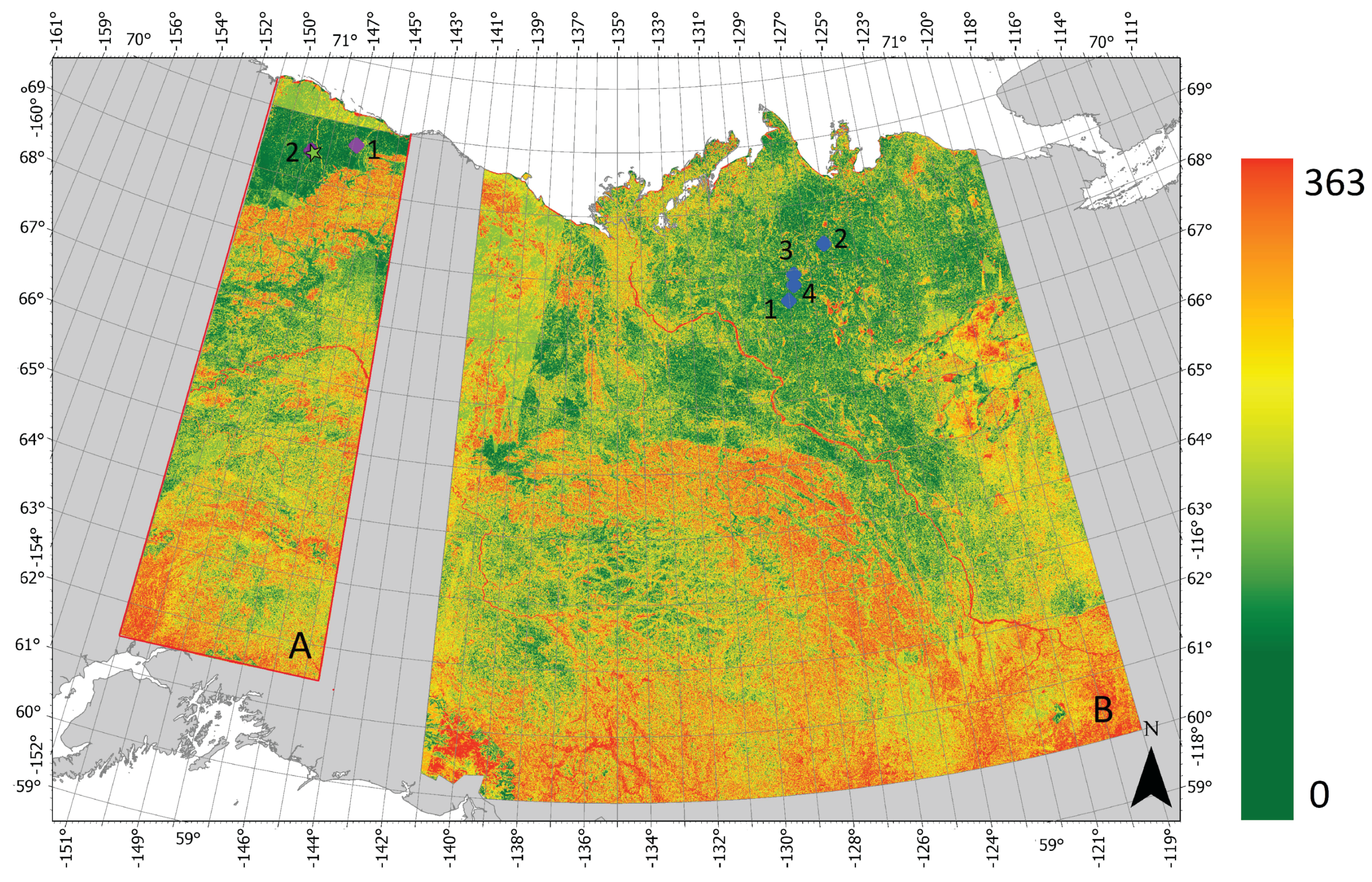
Extent of the surface state datasets; extent of circumpolar Advanced SCATterometer (ASCAT) dataset [42] visualized by the black rectangle (total map extent); extent of Advanced Synthetic Aperture Radar (ASAR) dataset [41] visualized by red polygons for the regions: Alaska (A); Mackenzie (B); Ob Estuary (C); Central Yakutia (D); Laptev Sea Coast (E); in Regions A, B and C, black dots symbolize selected ASCAT grid cells; colors correspond to landscape types (purple: tundra with partial floodplain; blue: lake dominated tundra; pink: tundra; green: forest).
Figure 1.
Extent of the surface state datasets; extent of circumpolar Advanced SCATterometer (ASCAT) dataset [42] visualized by the black rectangle (total map extent); extent of Advanced Synthetic Aperture Radar (ASAR) dataset [41] visualized by red polygons for the regions: Alaska (A); Mackenzie (B); Ob Estuary (C); Central Yakutia (D); Laptev Sea Coast (E); in Regions A, B and C, black dots symbolize selected ASCAT grid cells; colors correspond to landscape types (purple: tundra with partial floodplain; blue: lake dominated tundra; pink: tundra; green: forest).
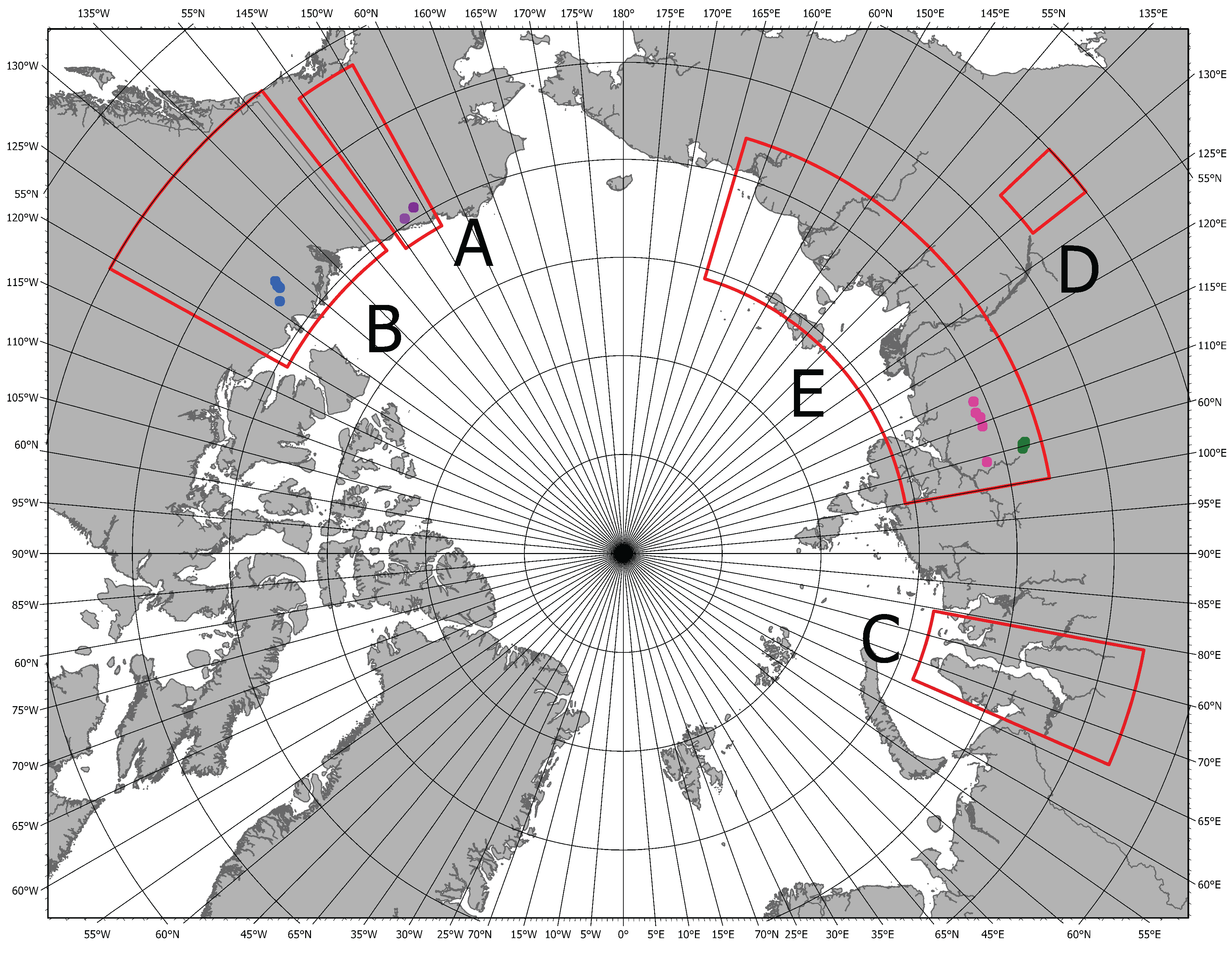
Figure 2.
Temporal discrepancies in freeze thaw data (SAR-ASCAT) between the ASCAT [42] and SAR [42] datasets for selected ASCAT grid cells in Alaska. The percentage of areas is given for all possible types of combinations between the two datasets (averaged for 2007–2010).

Figure 3.
ASAR acquisitions included in the freeze/thaw dataset [41] for the Ob Estuary in 2007–2010.
Figure 3.
ASAR acquisitions included in the freeze/thaw dataset [41] for the Ob Estuary in 2007–2010.

Figure 4.
Days of discrepancies (yearly mean) between the ASCAT [42] and SAR [42] datasets for the regions covered by the SAR dataset; Alaska (A); Mackenzie (B); squares represent selected grid cells, colors correspond to landscape types (purple: tundra with partial floodplain; blue: lake dominated tundra); the red outline around Region A indicates the extent of the terrain map (Figure 7).

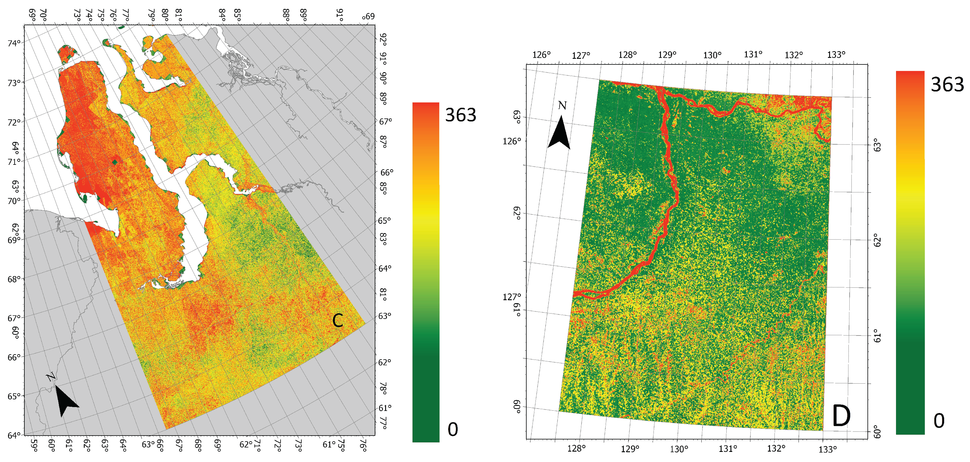
Figure 5.
Days of discrepancies (yearly mean) between the ASCAT [42] and SAR [42] datasets for the regions covered by the SAR dataset; Ob Estuary (C); Central Yakutia (D).

Figure 6.
Days of discrepancies (yearly mean) between the ASCAT [42] and SAR [42] datasets for the regions covered by the SAR dataset; Laptev Sea Coast (E); squares represent selected grid cells; colors correspond to landscape types (pink: tundra, green: forest).
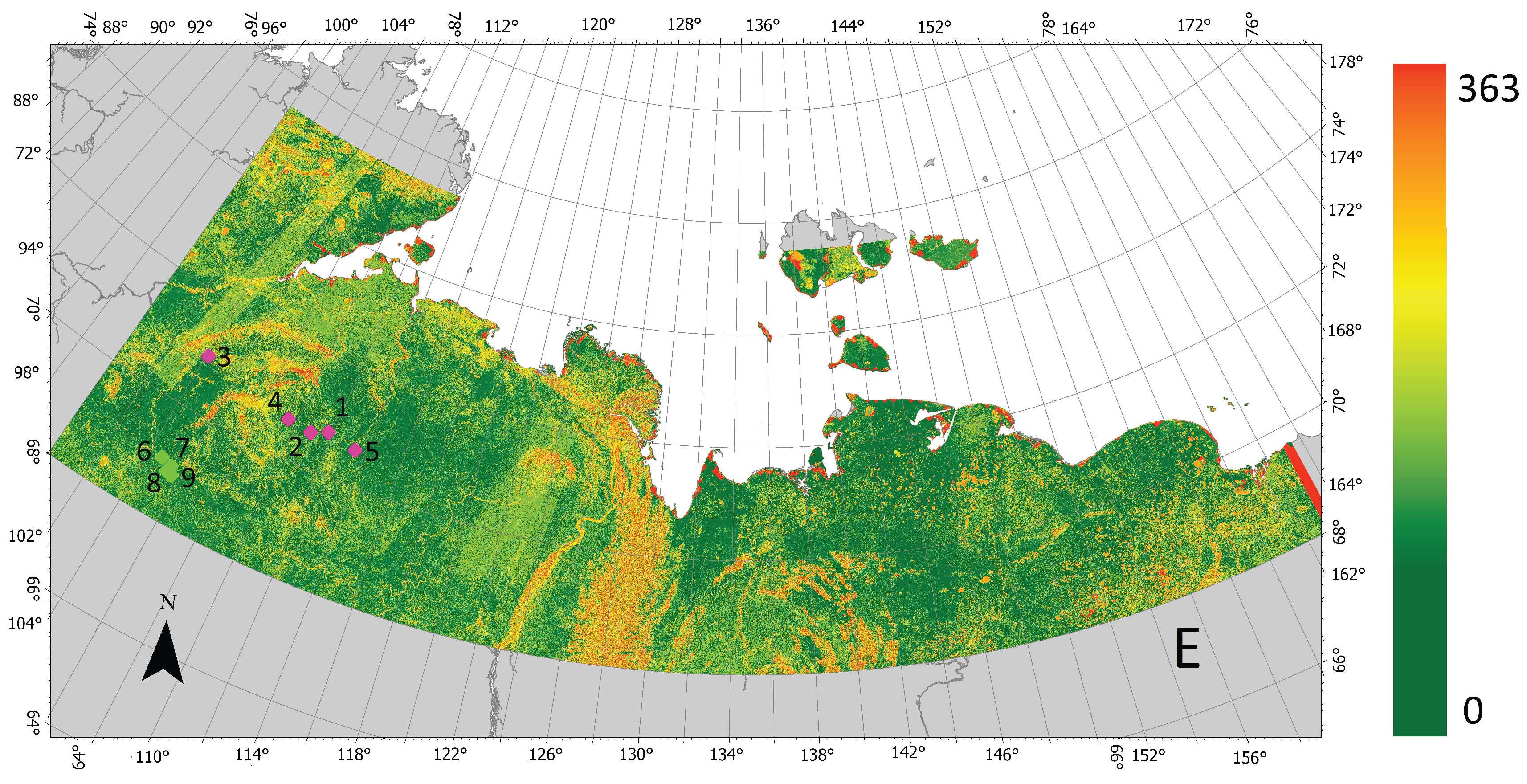
Figure 7.
Topographical map of area covered by SAR dataset, region Alaska (A) as in Figure 4.
Figure 7.
Topographical map of area covered by SAR dataset, region Alaska (A) as in Figure 4.
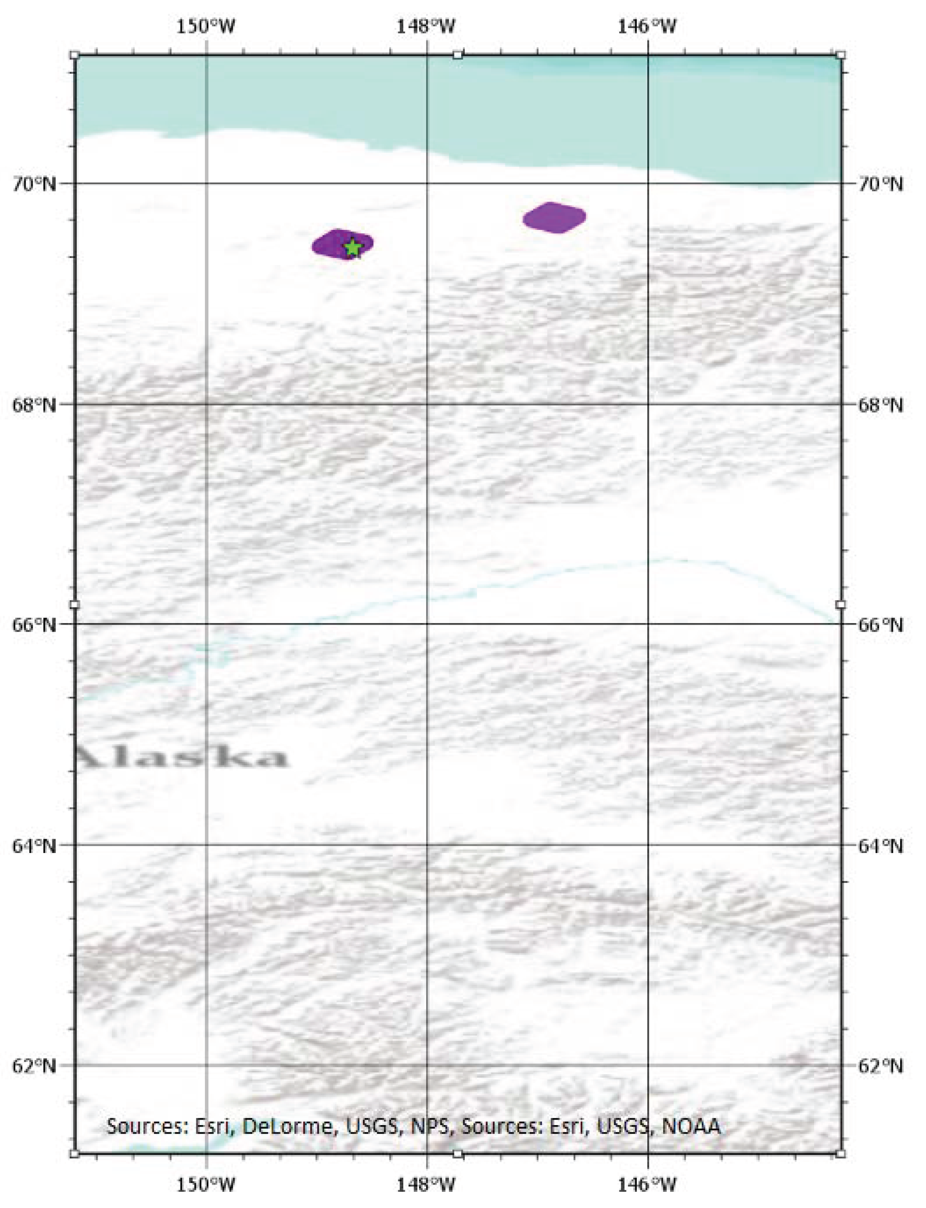
Figure 8.
Percentage of thawed SAR pixel within one ASCAT grid cell during transitional periods (indicated by the Day Of the Year (DOY)), including DOY of the last surface state change in the ASCAT product (red symbols) for the selected grid cells with no assigned landscape type (Alaska 1, Alaska 2), for the ASCAT [42] and SAR [42] datasets.

Figure 9.
Percentage of thawed SAR pixel within one ASCAT grid cell during transitional periods (indicated by the DOY), including DOY of the last surface state change in the ASCAT product (red symbols) for the selected grid cells with the assigned landscape type Lake dominated tundra (Mackenzie 1, Mackenzie 2, Mackenzie 3, Mackenzie 4), for the ASCAT [42] and SAR [42] datasets.
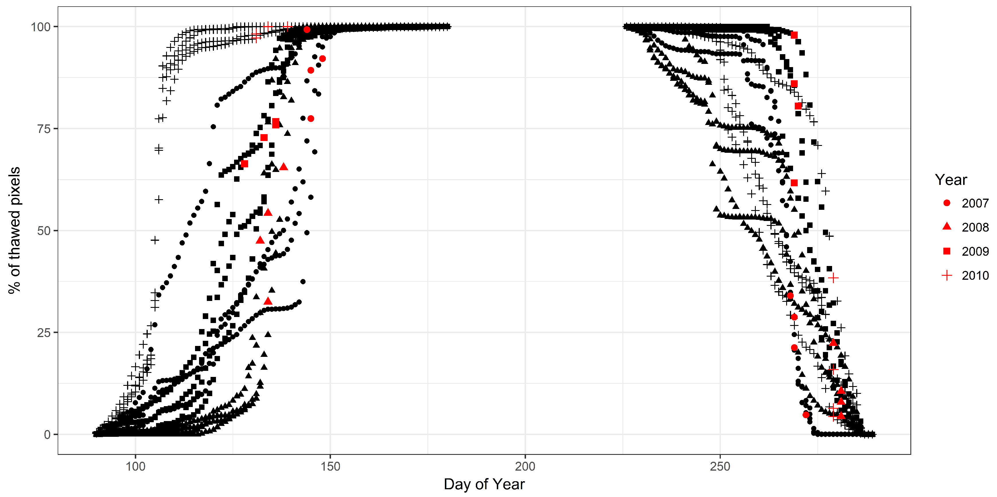
Figure 10.
Percentage of thawed SAR pixel within one ASCAT grid cell during transitional periods (indicated by the DOY), including DOY of the last surface state change in the ASCAT product (red symbols) for the selected grid cells with the assigned landscape type Tundra (Laptev Sea 1, Laptev Sea 2, Laptev Sea 3, Laptev Sea 4, Laptev Sea 5), for the ASCAT [42] and SAR [42] datasets.

Figure 11.
Percentage of thawed SAR pixel within one ASCAT grid cell during transitional periods (indicated by the DOY), including DOY of the last surface state change in the ASCAT product (red symbols) for the selected grid cells with the assigned landscape type Forest (Laptev Sea 6, Laptev Sea 7, Laptev Sea 8, Laptev Sea 9), for the ASCAT [42] and SAR [42] datasets.
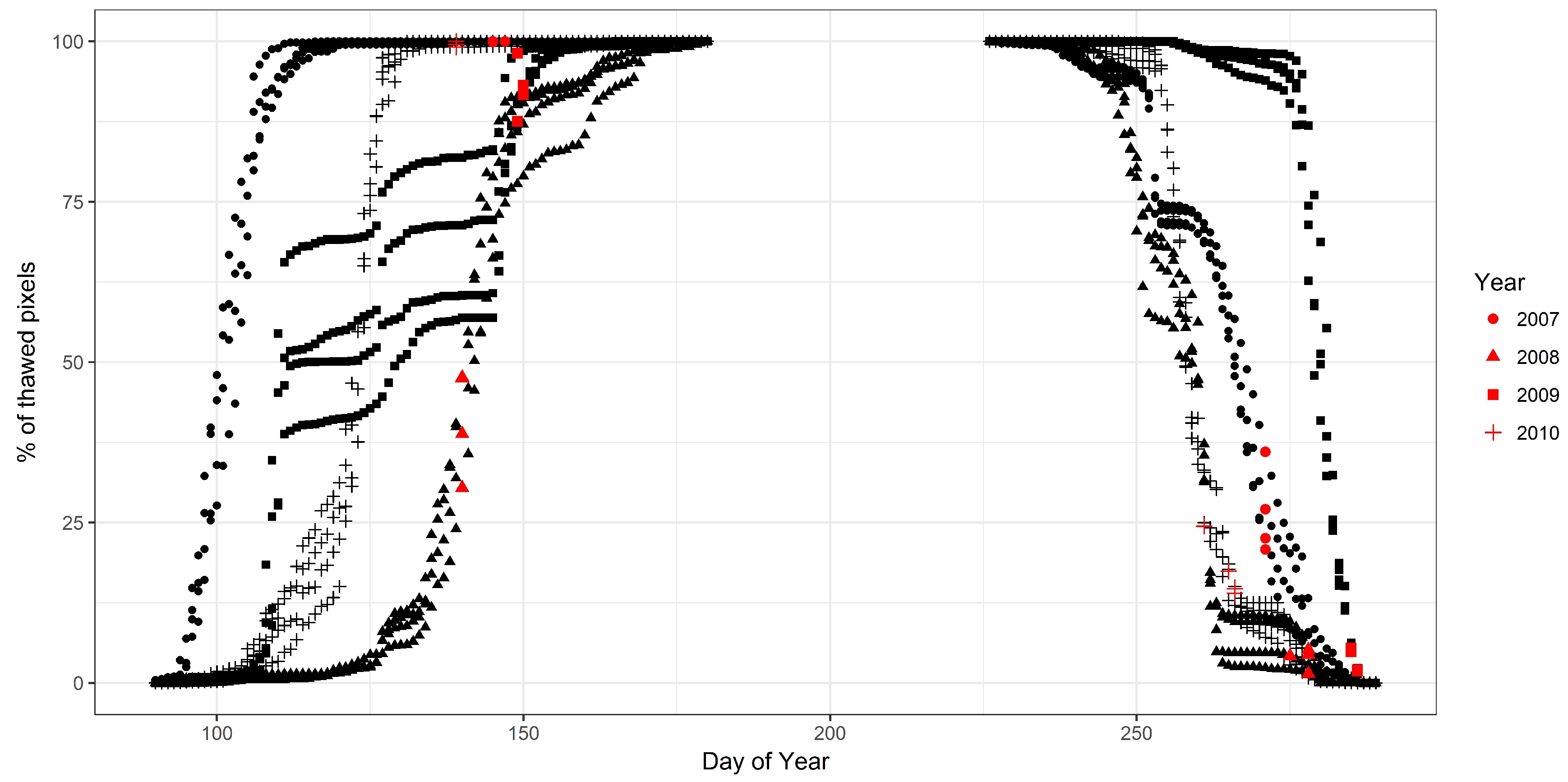
Figure 12.
Detailed view showing the % of thawed SAR pixels and the DOY for the ASCAT grid cell Laptev Sea 5 (type Tundra) for the years 2007–2010; based on the SAR [41] and ASCAT [42] freeze/thaw datasets; data are displayed from the last day of 0% thawed pixel each year to the first day of 100% thawed pixel each year; including a linear regression and a logistic fit with respective R2 and residual standard error (RSE).
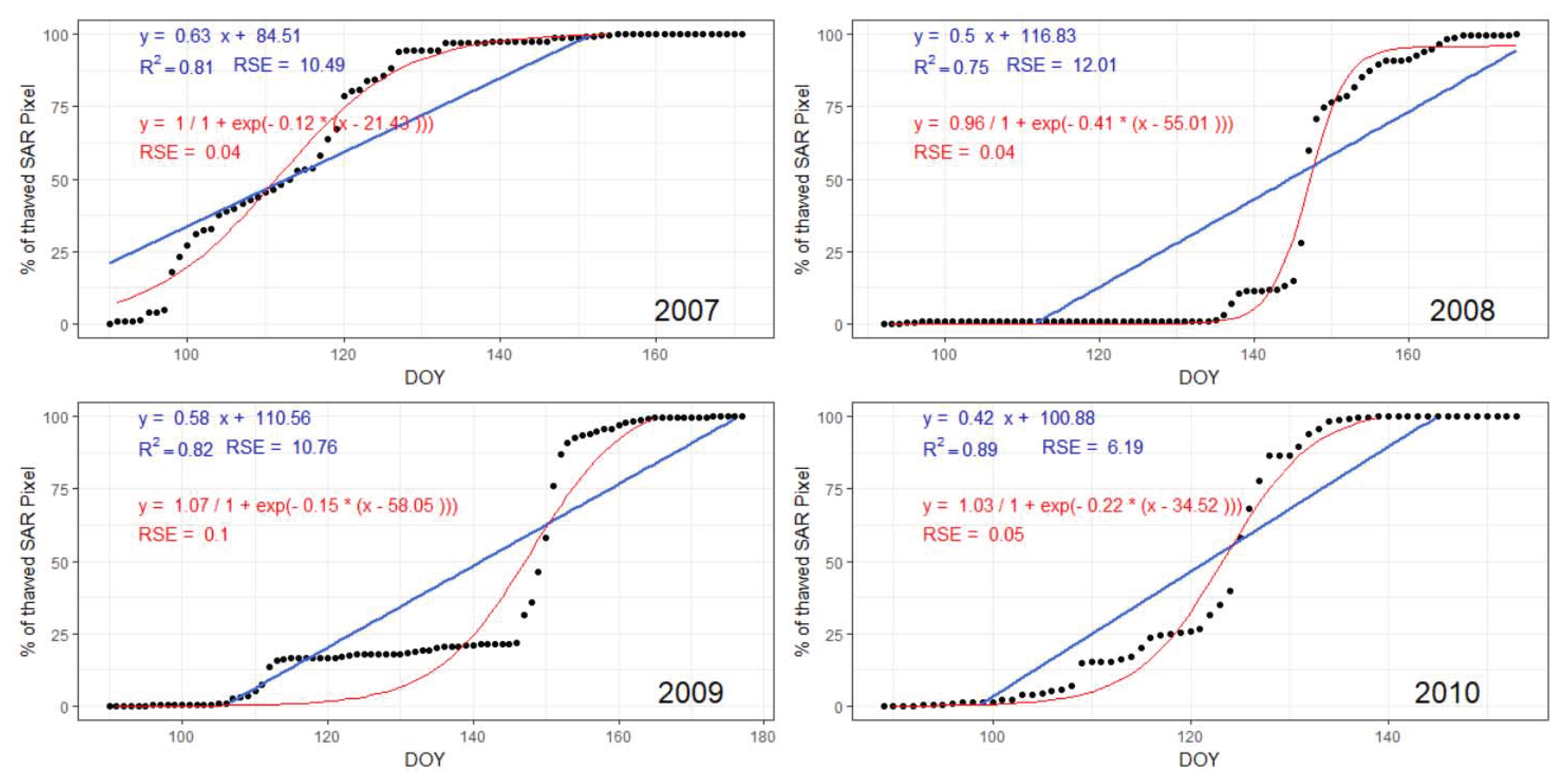
Figure 13.
Median, maximum and minimum of percentages of thawed and frozen SAR pixels (with black dots symbolizing outliers) within one ASCAT grid cell at the time of the last surface state change in spring and autumn in the ASCAT product for different landscape types, for the ASCAT [42] and SAR [42] datasets.

Figure 14.
Median, maximum and minimum of percentages of thawed and frozen SAR pixels (with black dots symbolizing outliers) within one ASCAT grid cell at the time of the first surface state change in spring and autumn in the ASCAT product for different landscape types, for the ASCAT [42] and SAR [42] datasets.

Figure 15.
Median discrepancy days between the ASCAT [42] and ASAR [41] datasets for all selected grid cells for spring and autumn in relation with median SAR coverage for all selected ASCAT grid cells for the years 2007–2010.
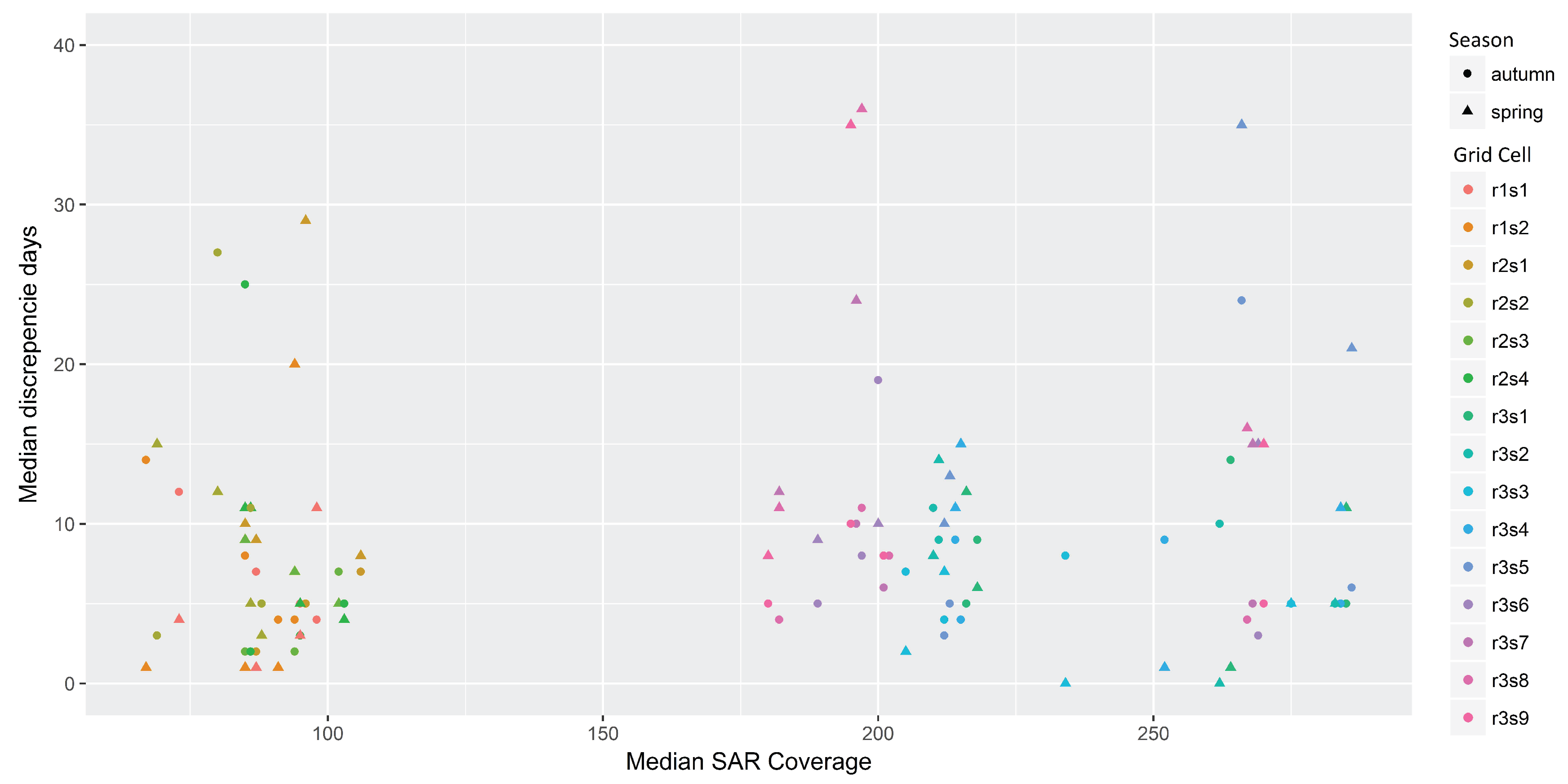
Figure 16.
Scatterplot of four-year mean values of discrepancy days between the ASCAT [42] and SAR [41] product for spring and autumn for all selected grid cells.
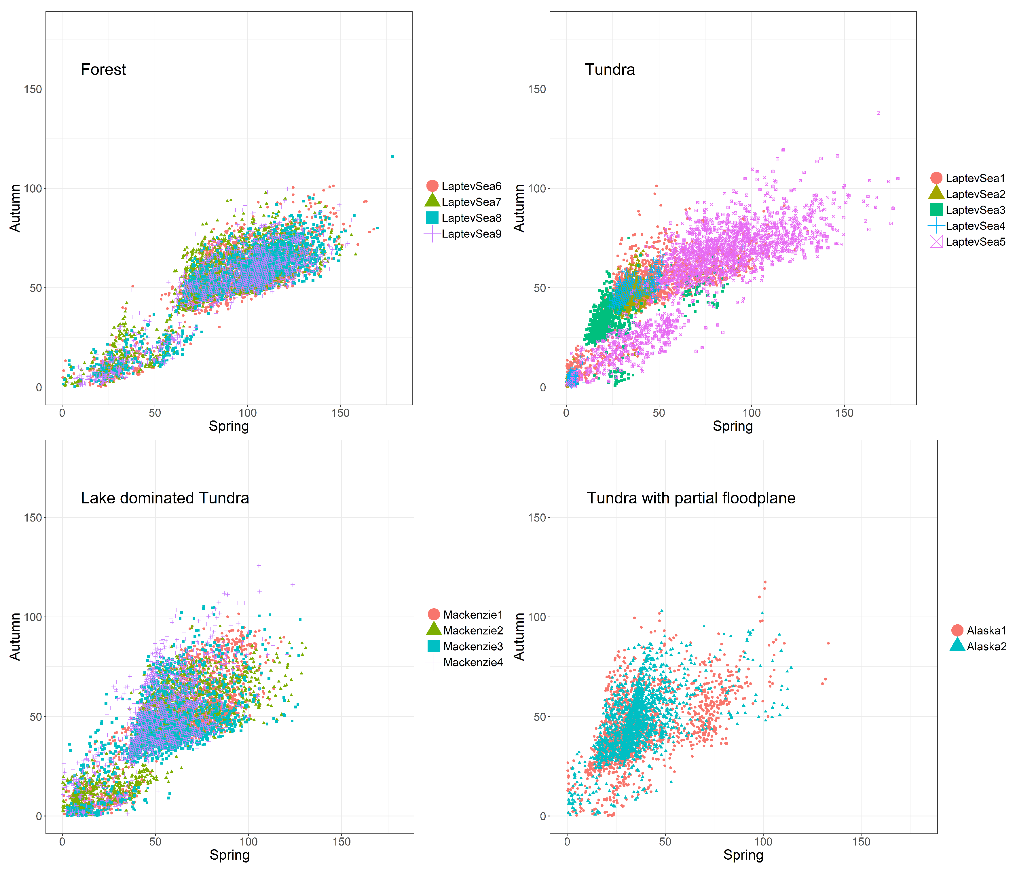
Figure 17.
Air and near surface soil temperature for Sagwon [54], ASCAT surface state change date for the corresponding grid cell (red), percentage of thawed SAR pixels within the ASCAT grid cell and SAR surface state change date for the location of the measurement site (blue).
Figure 17.
Air and near surface soil temperature for Sagwon [54], ASCAT surface state change date for the corresponding grid cell (red), percentage of thawed SAR pixels within the ASCAT grid cell and SAR surface state change date for the location of the measurement site (blue).


Table 1.
Selected Advanced SCATterometer (ASCAT) grid cells, including landscape type (Lake-dominated tundra: L; Tundra: T; tundra partially including Floodplain: FL; Forest: F), elevation range in meters [56], standard deviation of 4-year mean values for days of discrepancies in spring (SD Sp.) and autumn (SD At.) and average acquisition times for the Advanced Synthetic Aperture Radar (ASAR) and ASACT; the standard deviation is calculated using the sum of days of discrepancies between datasets on the SAR grid for spring (April, May and June) and autumn (September, October and November) 2007–2010.
| Site | Latitude | Longitude | Type | EL.Range | SD S. | SD A. | Av.ASAR Acqu.Times | Av.ASCAT Acqu. Times |
|---|---|---|---|---|---|---|---|---|
| Al.1 | 69.698 | −146.842 | FL | 147–328 | 21.25 | 17.17 | 6–8 a.m.; 8–10 p.m. | 04–7:30 a.m.; 7:30–11 p.m. |
| Al. 2 | 69.458 | −148.765 | FL | 149–360 | 14.63 | 14.85 | 6–8 a.m.; 8–10 p.m. | 04–7:30 a.m.; 7:30–11 p.m. |
| Mack.1 | 67.534 | −128.027 | L | 155–283 | 23.84 | 21.64 | 4–6 a.m.; 5–8 p.m. | 3–6 a.m.; 6–9 p.m. |
| Mack. 2 | 68.342 | −126.270 | L | 150–286 | 27.35 | 22.90 | 4–6 a.m.; 5–8 p.m. | 3–6 a.m.; 6–9 p.m. |
| Mack. 3 | 67.927 | −127.694 | L | 150–299 | 21.82 | 18.72 | 4–6 a.m.; 5–8 p.m. | 3–6 a.m.; 6–9 p.m. |
| Mack. 4 | 67.766 | −127.747 | L | 235–380 | 19.27 | 19.70 | 4–6 a.m.; 5–8 p.m. | 3–6 a.m.; 6–9 p.m. |
| Lap.Sea1 | 70.737 | 111.738 | T | 98–330 | 21.36 | 16.24 | 2–4 a.m.; 11 a.m.–3 p.m. | 2–5 a.m.; 9 a.m.–1 p.m. |
| Lap.Sea 2 | 70.607 | 110.869 | T | 375–508 | 7.64 | 7.58 | 2–4 a.m.; 11 a.m.–3 p.m. | 2–5 a.m.; 9 a.m.–1 p.m. |
| Lap.Sea 3 | 70.967 | 104.118 | T | 331–487 | 12.34 | 8.76 | 2–4 a.m.; 11 a.m.–3 p.m. | 2–5 a.m.; 9 a.m.–1 p.m. |
| Lap.Sea 4 | 70.657 | 109.495 | T | 429–606 | 15.62 | 17.93 | 2–4 a.m.; 11 a.m.–3 p.m. | 2–5 a.m.; 9 a.m.–1 p.m. |
| Lap.Sea 5 | 70.623 | 113.418 | T | 16–163 | 31.31 | 22.66 | 2–4 a.m.; 11 a.m.–3 p.m. | 2–5 a.m.; 9 a.m.–1 p.m. |
| Lap.Sea 6 | 69.023 | 104.712 | F | 180–328 | 27.65 | 17.19 | 2–4 a.m.; 11 a.m.–3 p.m. | 2–5 a.m.; 9 a.m.–1 p.m. |
| Lap.Sea 7 | 68.964 | 105.309 | F | 189–304 | 30.85 | 20.16 | 2–4 a.m.; 11 a.m.–3 p.m. | 2–5 a.m.; 9 a.m.–1 p.m. |
| Lap.Sea 8 | 68.853 | 105.228 | F | 179–272 | 27.77 | 17.52 | 2–4 a.m.; 11 a.m.–3 p.m. | 2–5 a.m.; 9 a.m.–1 p.m. |
| Lap.Sea 9 | 68.823 | 105.524 | F | 231-301 | 29.57 | 18.54 | 2–4 a.m.; 11 a.m.–3 p.m. | 2–5 a.m.; 9 a.m.–1 p.m. |
© 2017 by the authors. Licensee MDPI, Basel, Switzerland. This article is an open access article distributed under the terms and conditions of the Creative Commons Attribution (CC BY) license (http://creativecommons.org/licenses/by/4.0/).
Share and Cite
MDPI and ACS Style
Bergstedt, H.; Bartsch, A. Surface State across Scales; Temporal and Spatial Patterns in Land Surface Freeze/Thaw Dynamics. Geosciences 2017, 7, 65. https://doi.org/10.3390/geosciences7030065
AMA Style
Bergstedt H, Bartsch A. Surface State across Scales; Temporal and Spatial Patterns in Land Surface Freeze/Thaw Dynamics. Geosciences. 2017; 7(3):65. https://doi.org/10.3390/geosciences7030065
Chicago/Turabian StyleBergstedt, Helena, and Annett Bartsch. 2017. "Surface State across Scales; Temporal and Spatial Patterns in Land Surface Freeze/Thaw Dynamics" Geosciences 7, no. 3: 65. https://doi.org/10.3390/geosciences7030065
Note that from the first issue of 2016, this journal uses article numbers instead of page numbers. See further details here.