The Isopach Mapping of Volcanic Deposits of Mount Samalas 1257 AD Based on the Values of Resistivity and Physical Properties

Abstract

A detailed study had been conducted on the sediment of Mount Samalas’ volcanic eruption in 1257 AD. Using the framework of the reconstruction of the ancient eruption of Mount Samalas, the first step was to map and analyze the deposits of volcanic sediment. Secondly, we analyzed the effect of geomorphology and the distance function to the isopach thickness. The results show that a combination of methods allowed to provide a high resolution map of the distribution of the thickness of the volcanic deposits, both on the slope and in alluvial areas. Geo-electric survey results (both Vertical Electric Sound (VES) and 2D mapping) show consistent changes in the pattern of contrast resistivity layer interface, for all areas. The pattern changes in a row of the top layer, the high resistivity turned into the low. Furthermore, the second and third layer interface changes from low to the high resistivity. High resistivity on the top layer is interpreted as a layer of unconsolidated volcanic sediment. High resistivity values are range from 736 to 2000 Ohm.m on the top layer in the area of the slopes while in the area of alluvial, the resistivity values range from 20 to 958 Ohm.m. Generally, the volcanic deposits in the area of the slopes have a higher value of isopach (>17 m) than in areas of alluvial (<25 m). The geomorphology seemed to have no significant effect on the isopach value, particularly pyroclastic fallout. Such is the case with distance from the source to the site, which is not linear. The value of isopach increases westward from 21 to 31 km, in contrast to the East, which began to occur at a distance of 14 km to 21 km.

1. Introduction

Many scientists and common people had shown their interests in volcanic mountains since a long time ago, because volcanic areas are prosperous and provide plenty of resources for humans. The researchers were more concerned with the substantial fact that the volcanic eruptions represent humans’ life. Therefore, the science of the activities of a volcanic mountain is now being promoted in several aspects, including the evolution and the history of the volcanic system. The evolutional pattern and the volcanic historical system have to be read in a more careful manner. The patterns have to be predicted accurately to reduce the impacts on humans and the surrounding environment. Here we use Mount Samalas in the Rinjani Volcanic Complex in Indonesia as an example. The history and the volcanic system of Mount Samalas since its 1257 AD plinian eruption [1] can be identified from the sedimentary map and the spatial context. In the last two decades, the understanding of the sedimentation of volcanic plume has been growing significantly. The models of plume sediment have been elaborated and are synchronous with the field data [2]. Generally, sediment from a volcanic eruption contains both falls and current deposits. Both types of sediments supply an important insight related to the volcanic activities in the past, including the dynamics of eruption’s column. The main dangers of an eruption are the intensity and the scale of the eruption. The estimated value of the tephra fall volume is one of the essential keys to predicting how dangerous the eruption of a volcanic mountain is. However, the inadequate data from outcrops underestimate the calculation of the tephra volume. The potential solution to solve the problem is an availability of indirect investigations methods such as geophysical ones. This method can greatly help in the mapping of volcanic plume sediments at affordable/reasonable costs, especially the geoelectrical resistivity method.

In order to appraise the volcanic sediment, it is important to construct isopach maps. The combination of geoelectrical technique, rock outcropmapping, and drilling data are appropriate methods to solve this problem. The geoelectrical method has been widely used to investigate those matters beyond the superficial, such as geological, environmental, geotechnical, and hydrogeological matters [3]. The Vertical Electric Sound (VES) method has been used in differentiating the deposition of Quarter paleo-climate sediments [4]. VES application is used for mapping the pyroclastic thickness [5] on a morphological situation where the mountain slopes are steep and inaccessible as an affordable and flexible method. Shallow Quaternary volcanic sediment was measured using the geoelectric method [6].

The characteristics of volcanic sediment on the bedrock level obtained from VES data inversion showed a unit of high and low resistivity [7]. Bedrock is a solid rock exposed at the surface or underlying soil; has a shear-wave velocity greater than 795 m/s at small (0.0001 percent) strains.

The 2D mapping has been utilized to visualize the ventilation and the volcanic embankment, volcanic geological tuff contact, and basaltic rock [8].

The integrated information between geophysics and geology can be applied to characterize the sediment composition around lakes [9]. Is the combination of geophysical methods, outcrop observation, and drilling efficient for the isopach mapping of the volcanic sediment? Do the topographic condition and the distance from the crater influence the value of isopach?

2. Materials and Methods

In this research, vertical electrical sounding (VES) and electrical resistivity tomography (ERT) method are used.

2.1. Geological Background

Mount Samalas is located at the western side of Mount Rinjani, Lombok, Indonesia (Figure 1). As written in Babad Lombok [10], this very large eruption created the caldera named Segara Anak and produced large tens of cubic kilometers of pumice. The dimension of caldera Segara Anak is 6.0 km × 8.5 km and 0.2 km depth [11]. The other indication of the phenomenon is the existence of pumice fallout deposits which can be found in all parts of Lombok Island as well as thick Pyroclastic Density Currents (PDCs) deposits in some areas. Based on [12] the caldera was created in between 1210 and 1260 AD. Further studies succeeded to correlate this catastrophic volcanic event to the so-called 1257 AD “mystery eruption” found in polar ice cores [1,13].

Generally, volcanic sediment of Mount Samalas is divided into three main units, with massive characteristics, unsorted, and multi-model granule size [14]. Three basic types of volcanic deposits are falls, surge, and PDCs sediments. The characteristics of fall deposits involve: topographic coated, parallel bedding, well-organized, and opened gradation (very close to vent, particles fall vertically and reach broader scope). While the characteristics of flow sediment encompass limited topography, unorganized, and opened gradation. PDCs deposition’s characteristics are separated topography, cross-bedding, medium-opened gradation. PDCs sediment includes scoria (big-sized mafic), pumice (big-sized silica), and ash. This kind of deposit can be found almost everywhere and has the similar thickness in some distances and direction from the vent. Therefore, falls sediment became the topographic coating.

Volcanic deposits of Mount Samalas can be found in all parts of Lombok Island. The volcanic sediment constructed the stratigraphy of Lombok Island, particularly in Rempek, Sembalun, Sedau, and Korleko (Figure 1). Formation Qv is the ancient volcanic mountain rock and Quaternary Holocene-Pleistocene. Types of the rock are andesitic, alluvial, and sand sediment [15]. The composition of volcaniclastic at the western part of Mount Samalas especially in Tanjung and Pemenang area is Tqb and Qvl formation. So are the southern and eastern parts of Mount Samalas such as Narmada-Sedau, Masbagik, and Korleko.

The thick and wide deposits of Mt. Samalas are found in three main directions, namely to the NW, SW and SE. For example, the thickness of the PDC deposits reaches 34 m at Tebing Beach (NW), 20 m at Luk (NW), and 20 m at Ladon. The sediment sequence consists of three units: Ultraplinian, Plinian, and Phreatoplinian [1]. The third unit is covered by thick sediments containing pumice stone.

The variations of volcanic deposit were found in different locations, such as alluvial, and diagonal slopes according to the geomorphological state. The deposit showed that PDC was commonly precipitated in the horizontal slopes, while drop deposit turned into the topographic coating and can be found in almost all parts except the eastern part. The volcanic deposit in the coating form was commonly found in Qvl (undidifferentiated), TQb (Kalibabak formation), and TQp (Kalipalung formation) (Figure 1).

2.2. Methods

The distribution of the resistivity of subsurface can be determined by performing the geoelectrical measurements on the surface. This distribution is influenced by the mineral content, porosity and fluid saturation level in the rocks. In this research, electrical resistivity surveys have been used for mapping volcanic deposits. The resistivity measurements are made by injecting current into the ground through two current electrodes (C1 and C2 in Figure 2a) and measuring the resulting voltage difference at two potential electrodes (P1 and P2). Next, we calculated the apparent resistivity ($\rho \alpha$) value from the current (I) and voltage (V),

$$\rho \alpha =\kappa (\frac{V}{I}),$$

(1)

where κ is the geometric factor which depends on the arrangement of the electrodes, see Figure 2.

A geo-electric survey has been conducted in two stages and two different techniques: the acquisition of a VES and 2D mapping. Measurement of the VES data, using the hybrid configuration of Wenner-Schlumberger. The hybrid configuration of Wenner-Schlumberger is more sensitive to the vertical and horizontal direction compared with Wenner and Schlumberger, as well as the configuration of Dipole-dipole [16,17,18,19]. Therefore this hybrid configuration was chosen for use in this study.

Measurement using the hybrid configuration of VES Wenner-Schlumberger, where four electrodes arranged in a straight line: each one pair of electrode current and potential. The distance of the electrode current is constantly improved steadily until the measured potential difference is quite small. When a potential difference is small it has been reached, then the distance of the electrode potential is increased once, at least for the current electrode. Furthermore, the distance from the electrode’s current is increased again as before until the measured potential difference is small enough again. The distance of the electrode potential is increased again. The process of improving the current and potential electrode distance is repeated continuously until it reaches the maximum limit of the specified line. The system increased the distance of the electrode potential and current these are typical of this hybrid configuration Wenner-Schlumberger. What follows is a discussion of 2D mapping.

The 2D mapping is done using the configuration of Dipole-dipole multi channels (Figure 2b). The electrodes are laid out all at once in an array, then measuring potential difference and current or subsurface resistance. In one 2D mapping path, one to four arrays is done in a straight line at each location. 14 electrodes are overlaid (Figure 2b) between one array with the next array. The overlapping electrode covers a wider depth. The mapping is done continuously to the point of the nth datum. The dipole-dipole circuit has n = 1 to 8 with some dipole length (1 to 3) to cover the near surface area.

Measurements are made with forwarding and backward arrays. The forward array is somewhat similar but not exactly the same as backward. The measurement begins with the forward direction to the end of the track and then proceeds with the measurement from the end of the path without changing the array type to save time throughout the survey. In this measurement, the reciprocal arrangement or command file switches the transmitter and receiver for a pair of forwarding and reciprocal measurements to check the quality of the data. Locations of our measure include three regions: Mataram region, Tanjung region, and Korleko region. The data VES acquisition by using a GSound tool and 2D mapping using a SuperSting R8 tool (AGI, Austin, TX, USA). The positions of every measurement were observed by using Global Positioning System (GPS) and an Inclinometer to obtain the accurate locations. This was crucial when interpreting the geoelectric data precisely.

VES data was acquired from 9 to 16 November 2015. The track of VES measurement was from the southeast to the northwest as represented by the triangles in Figure 1. The acquisition was performed from the southeast including Krumut beach, Tirpas, Ladon-Masbagik, Kembang Kerang, and Karang Baru. Meanwhile, the northwest areas included Luk, Sambik-Bangkol (call Samba), and Sanjajak. The distance between the acquisition location of VES ± 2 km and three sounds were occupied for each location. The distance between the sounding was 20 m to 30 m and put in a straight line. Thus, there were 24 soundings spots and the length of the minimum array (AB/2) was 75 m and a maximum of 150 m. The array’s length was suited to the field conditions and the approximate depth of the target, as well as the relative length (50–200) m as recommended [16].

The acquisition of 2D mapping was conducted from 1–9 August 2016. The 2D data acquisition was acquired in Mataram and the surrounding area (21 lines), in the region of Tanjung (9 lines) and 5 lines in the area of Korleko. The location of all these lines is indicated by red circles (Figure 1). The 2D Data Acquisition used the SuperSting R8 tool with digital continuous recording systems and 56 steel electrodes (stainless steel). These electrodes were assembled and inserted into the ground with fixed electrode spacing and connected to the multi-core cable. 2D mapping data acquisition lines were performed perpendicular with the alignment of the sediment. Spaced electrodes were adjusted to the approximate depth of the target and the field conditions. In the 2D mapping, the Dipole-dipole configuration was used, with variations of electrodes’ spaces: 1.5, 2.5, 3, 4, 5, and 10 m. The maximum length of the array in one measuring was 550 m. In each location, measurements were performed with three arrays and in a straight line with an overlap of 14 electrodes. The minimum length of measurement path for each was 82.5 m and a maximum of 1390 m.

Beside the geoelectric measurements (VES and 2D mapping), we had analyzed four outcrops, OC (Figure 1) and performed two boreholes, BH (Figure 1). The outcrops area at Tebing beach and Luk are described in

Table 1. Description of outcrops PDCs at Lokok Meang-Luk (±20 m high), OC-3 (Figure 1 and Figure 13a).

Lithology	Thickness (m)
Cl, Pu: Clay, pumice	5
Pu: Pumice	0.8
As, ig: Ash, ignimbrite	6
As, pu, ig: Ash, pumice, ignimbrite	8
Pu, ig: Pumice, ignimbrite	5
Pu, Sa, As: Pumice, Sand Ash	1
Pu: pumice Pu, Sa, As: Pumice, Sand, Ash	3
Cl, st: Clay stone	~

and

Table 2. Description of outcrops PDCs on Tebing Beach (height ± 34 m), OC-4 (Figure 1 and Figure 13b).

Lithology	Thickness (m)
Clay, pumice	5
Graind pumice	7
Sand	5
Pumice, sand	5
Sand Coarse pumice	6
	5
Sand	~

in Section 3. While the Samba and Krumut beach outcrops are displayed in Figure 3, Figure 4, Figure 5 and Figure 6. Drilling was also conducted at two research sites where outcrops were not available. It was on the Antareja street, Mataram (BH-1 in Figure 1) and in Jeranjang, West Lombok (BH-2 in Figure 1). The depth of drilling was based on the analysis of geoelectric respectively in the Antareja 21 m (Figure 6) and it samples described in

Table 3. Description of samples lithology was acquired at Antareja, Mataram. (403,754, 9,050,304) UTM (see BH-1 in Figure 1).

Depth (m)	Description of Lithology	Interpreted Resistivity (Ohm.m)
0.00–1.00	Clays	32–41
1.00–2.00	Sand, clay, gravel, grain pumice	103–205
2.00–10.00	Sand, clay, grain pumice	205–809
10.00–11.00	grain pumice
11.00–12.00	grain pumice, sand
12.00–13.00	Block fine sand, grain pumice	52–407
13.00–14.00	Block fine sand, mud	26–41
14.00–15.00	Block fine sand, mud
15.00–21.00	Mud, sand	6–23

and in Jeranjang 10 m depth (Figure 7) and its samples are described in

Table 4. Description of samples lithology was acquired at Jeranjang, West Lombok. (398,963, 9,042,313) UTM (see BH-2 in Figure 1).

Depth (m)	Description of Lithology	Interpreted Resistivity (Ohm.m)
0.00–1.00	Clays	52–103
1.00–2.00	Sand, clay, gravel, grain pumice	32–60
2.00–3.00	Sand, clay, grain pumice
3.00–4.00	Fine sand, grain pumice
4.00–9.00	Sand, mud, grain pumice
9.00–10. 00	Sand, coarse grain pumice
10.00–11.00	Clay, grain pumice

.

2.3. Processing Data VES and 2D Mapping

Observation data of geoelectric field were processed, interpreted and validated with data drill or outcrops. To get the model parameters (depth and resistivity) resistivity data VES and 2D ERT are modeled and invereted. The inversion of resistivity data modeling is done by using 1-D and 2-D ERT algorithms. The inversion process is implemented using Res2Dinv software (Geotomosoft Solutions, Penang, Malaysia) and IP2Win (Geoscan-M-Ltd, Moscow State University, Moscow, Russia).

Advanced modeling data was constructed from the observation of resistivity. The models were built from blocks with the assumption that each block had a constant resistance value and different from other blocks, in both vertical and horizontal directions. Advanced modeling was obtained by calculating the resistivity of pseudo-section. This advanced model was occupied as initial data in the inversion process.

Inversion means the estimation of subsurface model parameters (resistivity and thickness) based on experimental resistivity data. The inversion was executed by using the finite difference method and the initial data resistivity and the “prior information” from the drilling data or outcrops. Apparent resistivity was calculated in accordance with the respective electrodes space and trajectory configuration. Theoretical resistivity data is compared with the observed pseudo resistivity data, as described in the linear or nonlinear systems below.

All the pseudo-inverted resistivity data used L2-norm also known as least squares method [17] and quadratic optimization method [24,25]. If root means square (RMS) (Equations (3) or (5) or (6)) is still high (>5% or 10%) then the inversion process is tried again. To minimize this difference can be done using different approaches (Gauss-Newton approach, Tikhonov regularization strategy, and Occam’s strategy) to obtain smooth model parameters (i.e., the real resistivity estimate of the subsurface materials). The standard method of Gauss-Newton optimization, Tikhonov regularization strategy, and Occam’s strategy was used to limit the convergence error (5–10%). Jacobian matrix (Equation (3)), Taylor’s theorem (Equation (4)) or the damped least squares (Equation (5) or Equation (6)) was recalculated to obtain the most optimal resolution model. For more details see the linear system and nonlinear system the next discussion.

2.4. A Linear System

Considering a discrete linear problem we begin with a data vector d of m observations and a model vector m of n model parameters that we wish to determine. The inversion problem can be written as a linear system of Equation (2).

d = Gm

(2)

In some problems, the number of unknowns is more than the number of parameters (over-determined problems). A common way to estimate a model is to seek the model m that gives the best fit to the data in the sense that the difference, measured by the L2-norm, between the data vector d and the recalculated data Gm, is made as small as possible. This means that the least-squares solution is given by the model that minimizes the following cost function.

s = [d−Gm]²

(3)

This quantity is minimized by the following model estimate m = (G^TG)⁻¹G^Td.

2.5. Nonlinear Inversion Algorithm

Occam’s inversion Technique (2) with a higher-order Tikhonov regularization, inversion procedure contains two fundamental components. First, an algorithm (forward engine) is required to construct a theoretical dispersion curve based on the properties of an assumed profile. Second, an algorithm is required to minimize the objective function which is usually the error between the theoretical and experimental dispersion curves plus a damping term [22,25,26].

As the first step of inversion process, we need to linearize the nonlinear Equation (1). Given a trial model m^k approximation, Taylor’s theorem is applied to obtain the local approximation,

G(m^k + Δm) ≈ G(m^k) + J(m^k) Δm = d

(4)

where J(m^k) is the Jacobian matrix.

Suppose that we have a discrete n-point model m and discrete m-point data vector d that are related to a nonlinear system of equation G(m) = −d. We can formulate this problem as a damped least squares problem. The solution is given as

m^k+1 = (J(m^k)^T J(m^k) + α²L^TL)⁻¹ J(m^k)^Td(m^k),

(5)

where L is the roughening matrix and α is the damping factor.

The damped least squares solution for Q = 1 would be in the form of

m^k+1 = (QJ(m^k)^T (QJ(m^k)) + α²L^TL)⁻¹ (QJ(m^k))^TQd(m^k),

(6)

The flowchart of Occam’s inversion which implemented is:

• Set initial model (apparent resistivity, thickness).
• Calculate the theoretical curves G(m^k) and Jacobian matrix J(m^k) of the current model.
• Set a range of damping parameters (α α₁ α₂, α₃...).
• For each damping parameter α: (a) calculate and save a new model m^k+1 (6); (b) and the corresponding RMS errors RMS^k+1(α_i).
• Select the model m^k+1(α_i) based on the following criterions: if two or more trial models give RMS errors below a user-specific threshold ε₁: the largest α is preferred if no such values exist, then pick a value of α_i that minimizes the RMS^k+1(α_i).
• Check the model m^k+1(α_i) for convergence, in another word, check that the RMS^k+1(α_i) is small than a user-specific threshold ε₂.
• If the model does not converge, pass the model to next iteration (Step 2) until maximum iterations reached.

3. Results

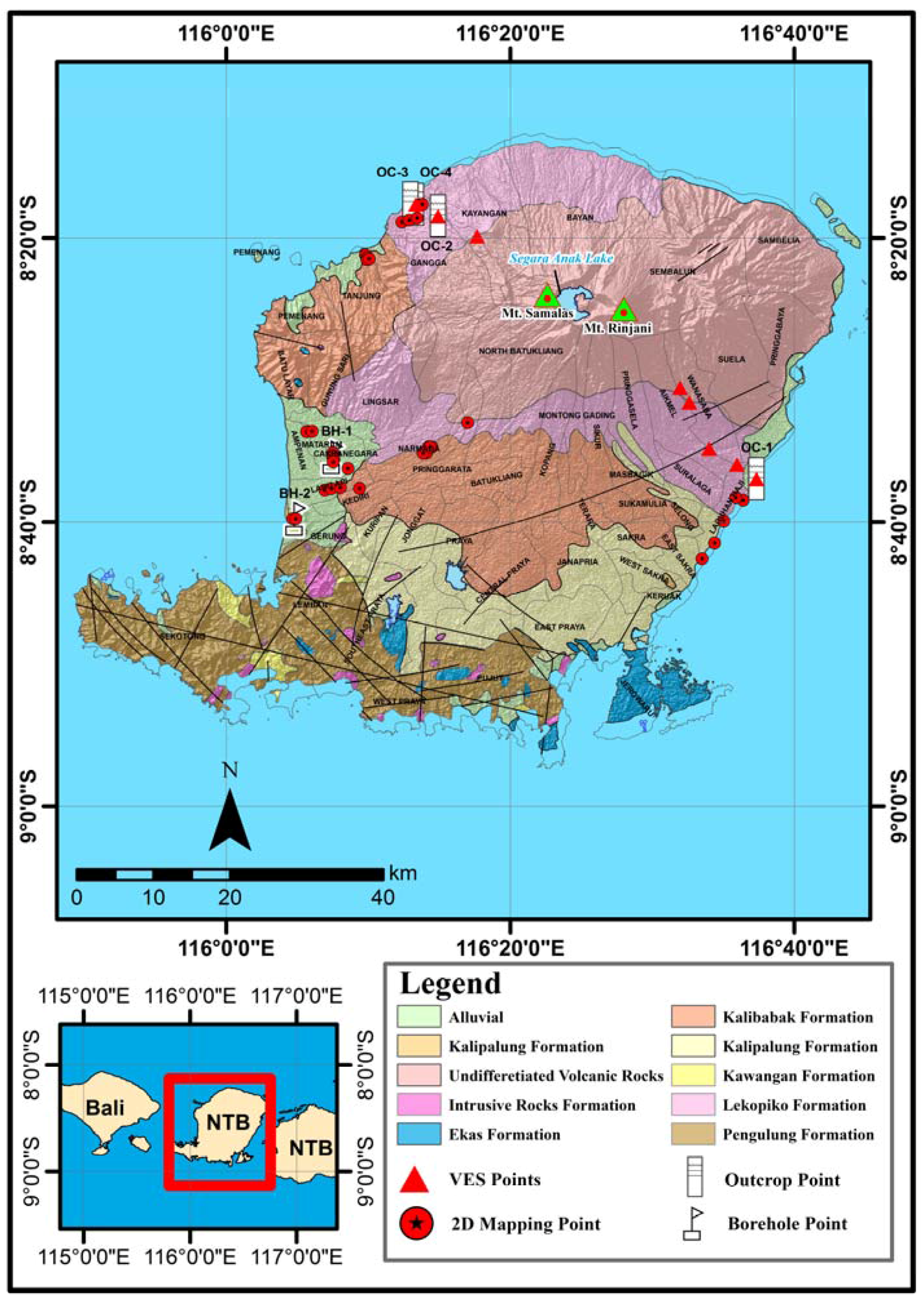
Field observation data, which had been inverted form VES resistivity, is shown in Figure 3 and Figure 5. Meanwhile, the depth profile (Figure 3) and resistivity logs (Figure 6) was constructed from the VES inversion. Figure 7, Figure 8 and Figure 9 are cross-sectional 2D ERT. 2D mapping was conducted in Mataram, Tanjung, and Korleko. Table 3 and Table 4 and Figure 7 and Figure 8 describe samples BH-1 and BH-2 (Figure 1 and Figure 10) in Antareja, Mataram, and in Jeranjang, West Lombok. Furthermore, the data inversion results were interpreted, validated, and then analyzed to create an isopach map as in Figure 10. The next job was to analyze the geomorphological effects on the isopach value to create an isopach profile of the Lombok Island (Figure 11). While the distance to the source of isopach site was used to analyze the profile distance function of the isopach to the source (Figure 12).

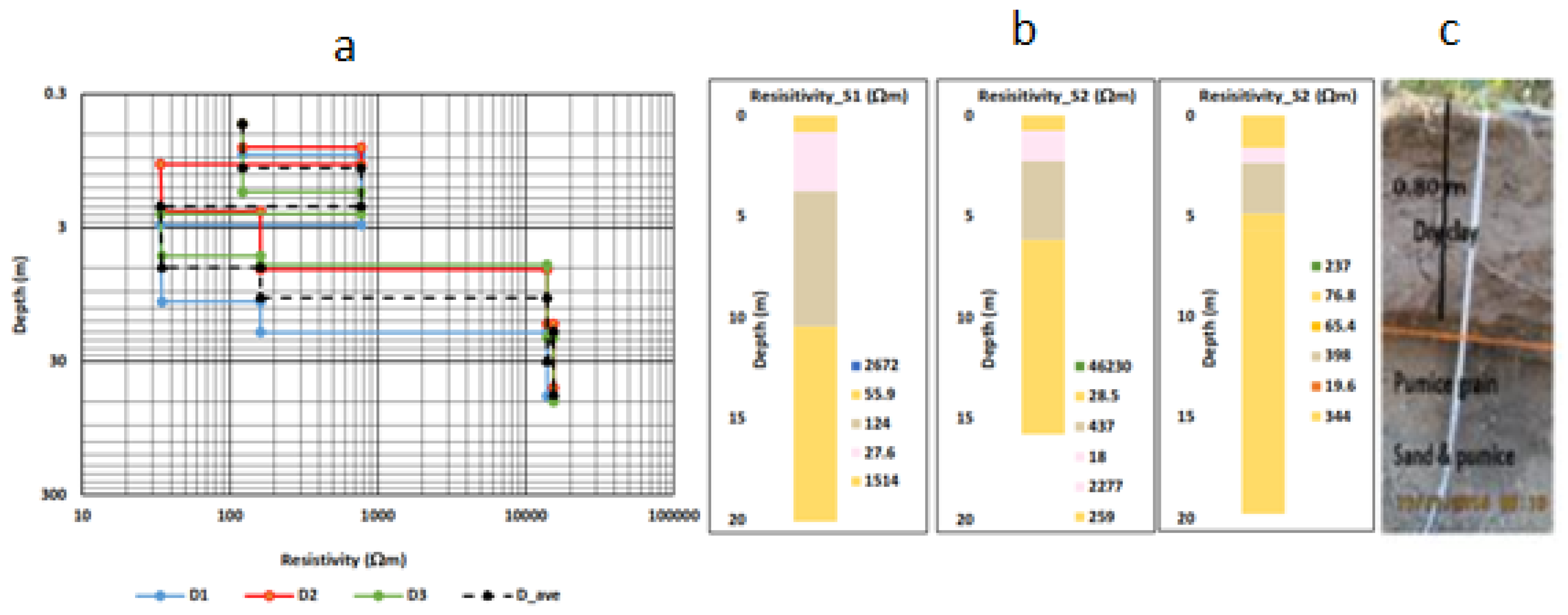
VES data which had been processed (Figure 3 and Figure 5) were validated by the outcrop-based observations (Figure 3b and Figure 5b). Thus, the actual value of the resistivity and thickness of each layer were then obtained. Profile depth as shown in Figure 3 was the result of the correlation of the three 1D inversion models S1, S2, and S3 (Figure 3). 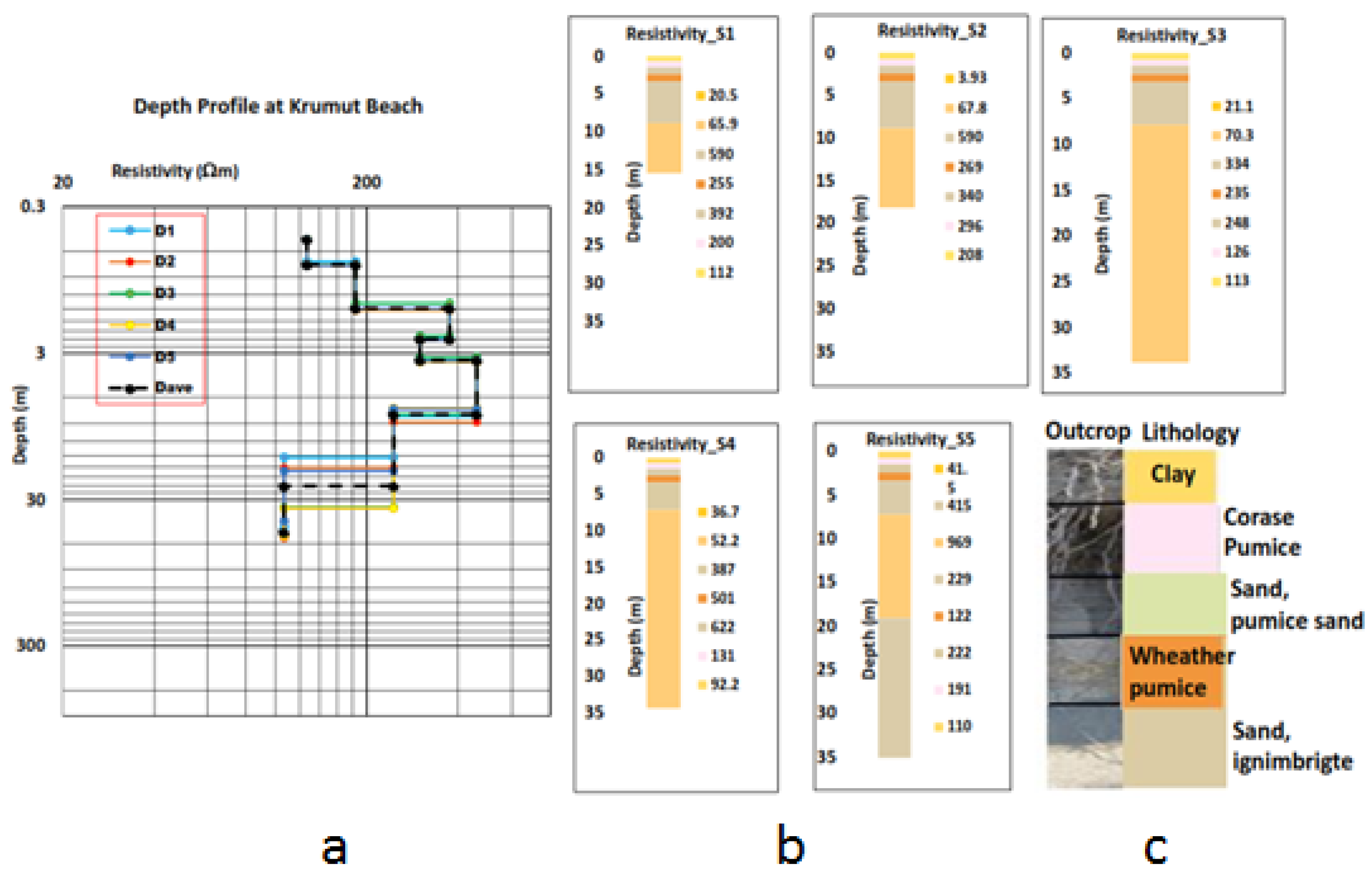The value of each of the three 1D inversion models (Figure 4b), was synchronized with the Log lithology (Figure 4c). Five resistivity soundings were conducted in Krumut beach (Figure 5) in the same manner, obtaining the in-depth resistivity profile (Figure 6a), which matched with the outcrop (Figure 5b), and then the average Log-resistivity was obtained (Figure 6b).

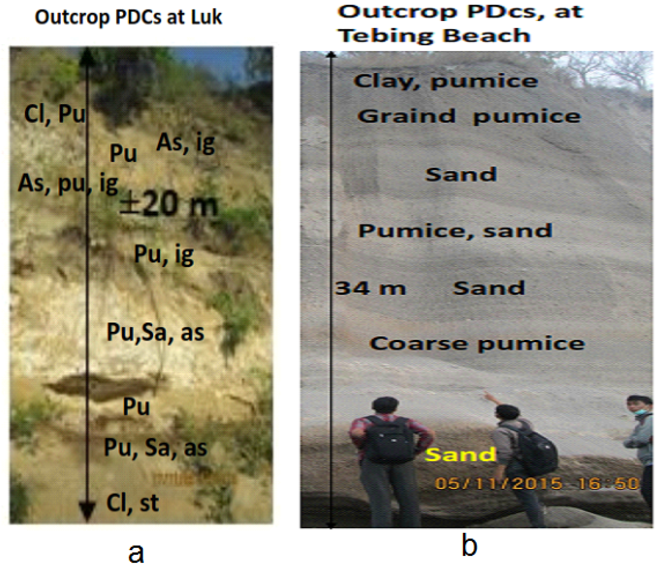
PDCs outcrop stratigraphy in Lokok Meang-Luk and Tebing Beach is shown in Table 1 and Table 3. The outcrop stratigraphy is composed of rocks: clay, coarse and fine pumice, sand, and ignimbrite inserts (Table 1 and Table 2). The strata layers were alternating between clays, pumice, sand ignimbrites inserts.

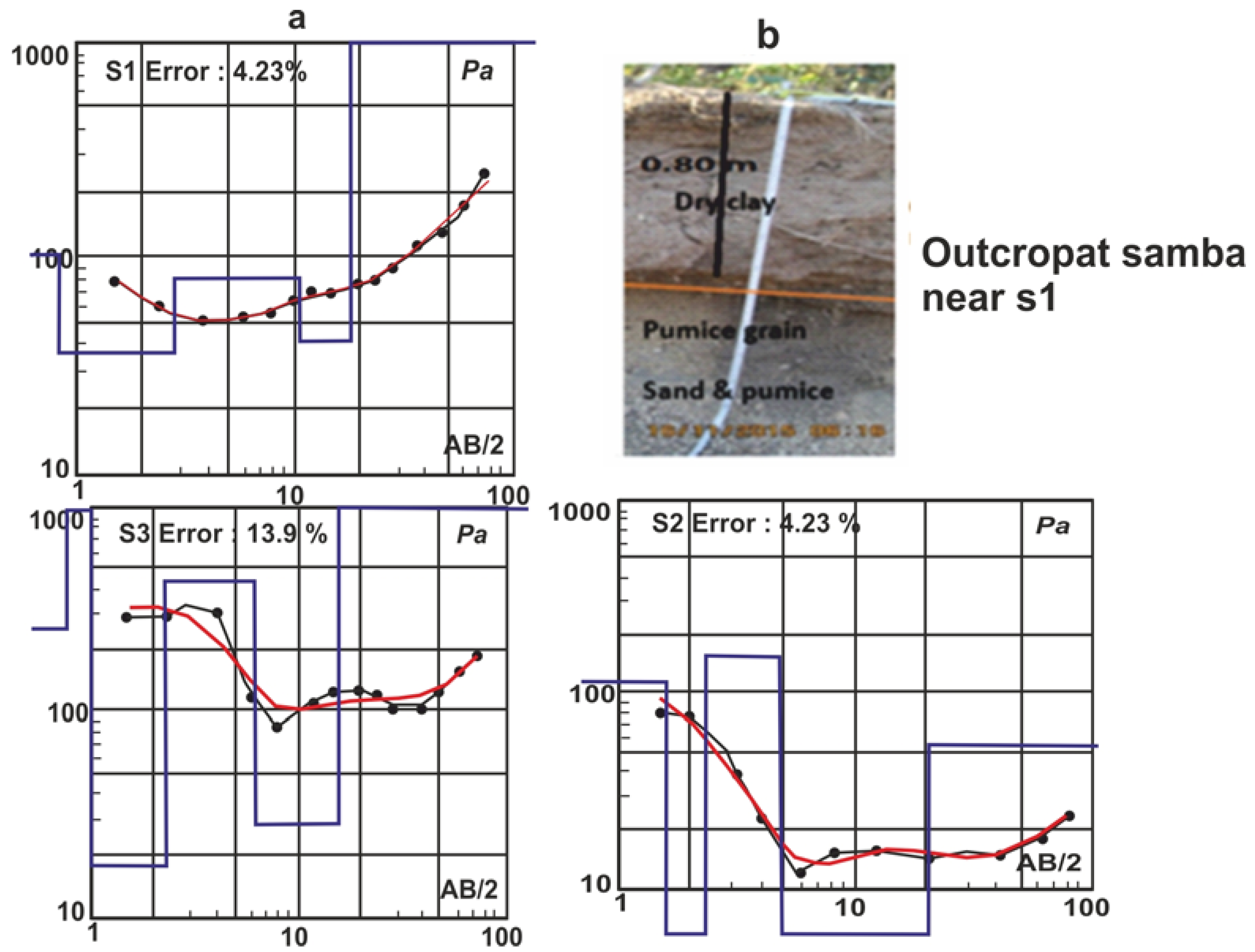
The results of VES data inversion in Figure 2 and Figure 3, were interpreted as follows: the first layer with a resistivity of 706 Ohm.m value was dry clay with pumice stone inserts (outcrop of 0.80 m thick, close to the calculated average, 1.06 m). The second layer corresponds to granular pumice with 1.30 m thick and 775 Ohm.m of detainees’ value. The third layer was composed of sand and pumice stone inserts, with a thickness of 2.48 m and resistivity value of 180 Ohm.m. Next was a mud layer with a pumice stone inserts, a thick layer of 5.66 m and resistivity value of 186 Ohm.m and an average depth of 9.14 m. The fifth layer was a 11.86 m thick claystone with resistivity values of 926 Ohm.m and was located at a depth of 17.52 m. The outcrop in Figure 3 and Figure 4 was located near the audible S1.

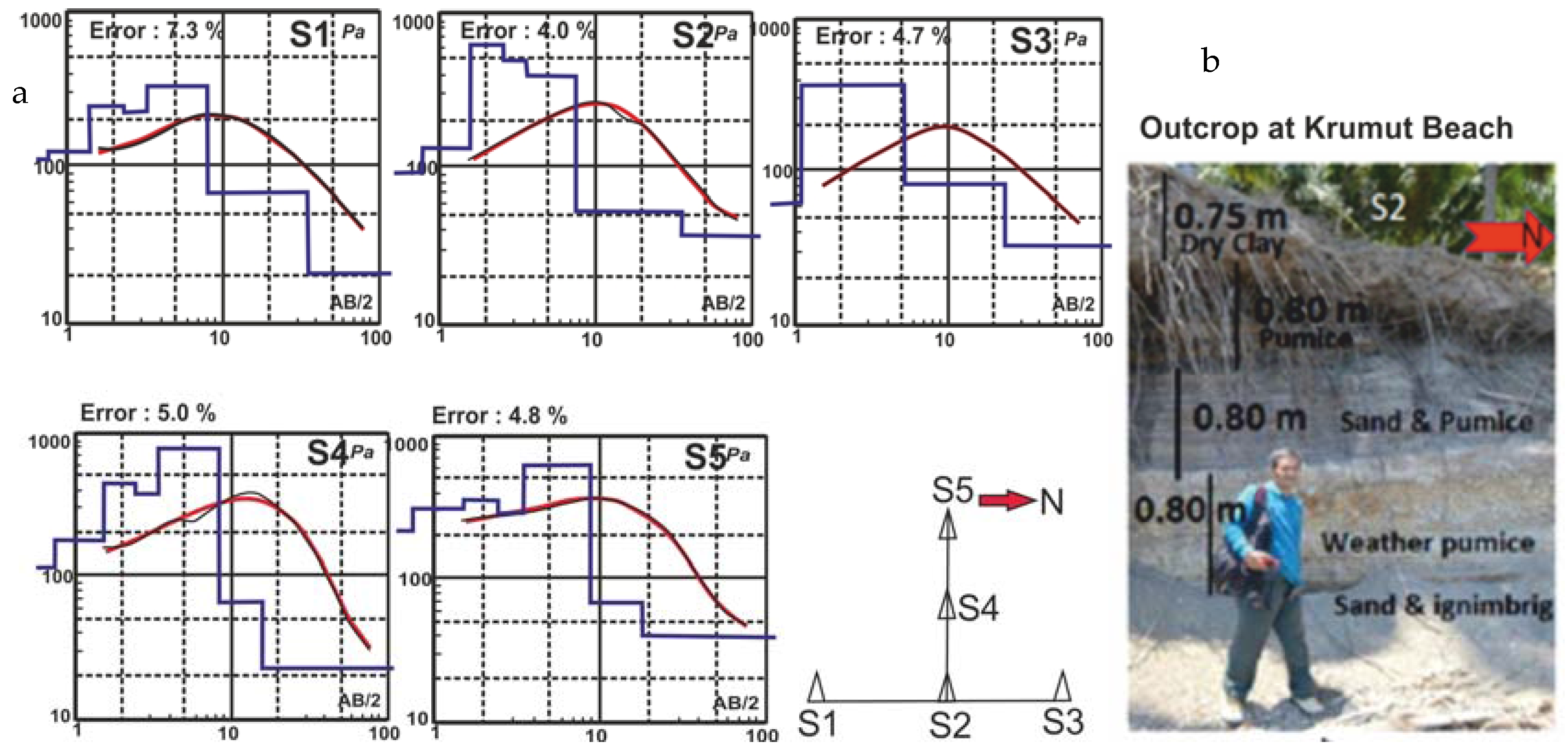
Profiles in Figure 5a showed the bedding level of Krumut beach a 0.75 m thick layer of clay with resistivity value of 127.04 Ohm.m (Figure 5b). The second layer consists of pumice with a resistivity value of 188.80 Ohm.m and thickness of 0.73 m (0.80 m on outcrop). The thickness of the third layer is 0.92 m (0.80 m thick) and 364.80 Ohm.m in resistance value which consists of alternating layers of sand with a thin layer of pumice sand. The fourth layer was filled by a thick layer of pumice by 0.95 m (0.80 m on riel value) and resistivity value of 276.40 Ohm.m. The fifth layer had a resistivity of 447.60 Ohm.m and 4.62 m thick sand and ignimbrite insert, and the sixth layer, defined as a rock with a thick clay 16.20 m and 245.04 Ohm.m. The innermost layer (23.21 m) had a resistivity value of 99.45 Ohm.m which could be detected and interpreted as sandstone. The next job was to interpret the 2D mapping data, as many as 35 lines at 9 locations.

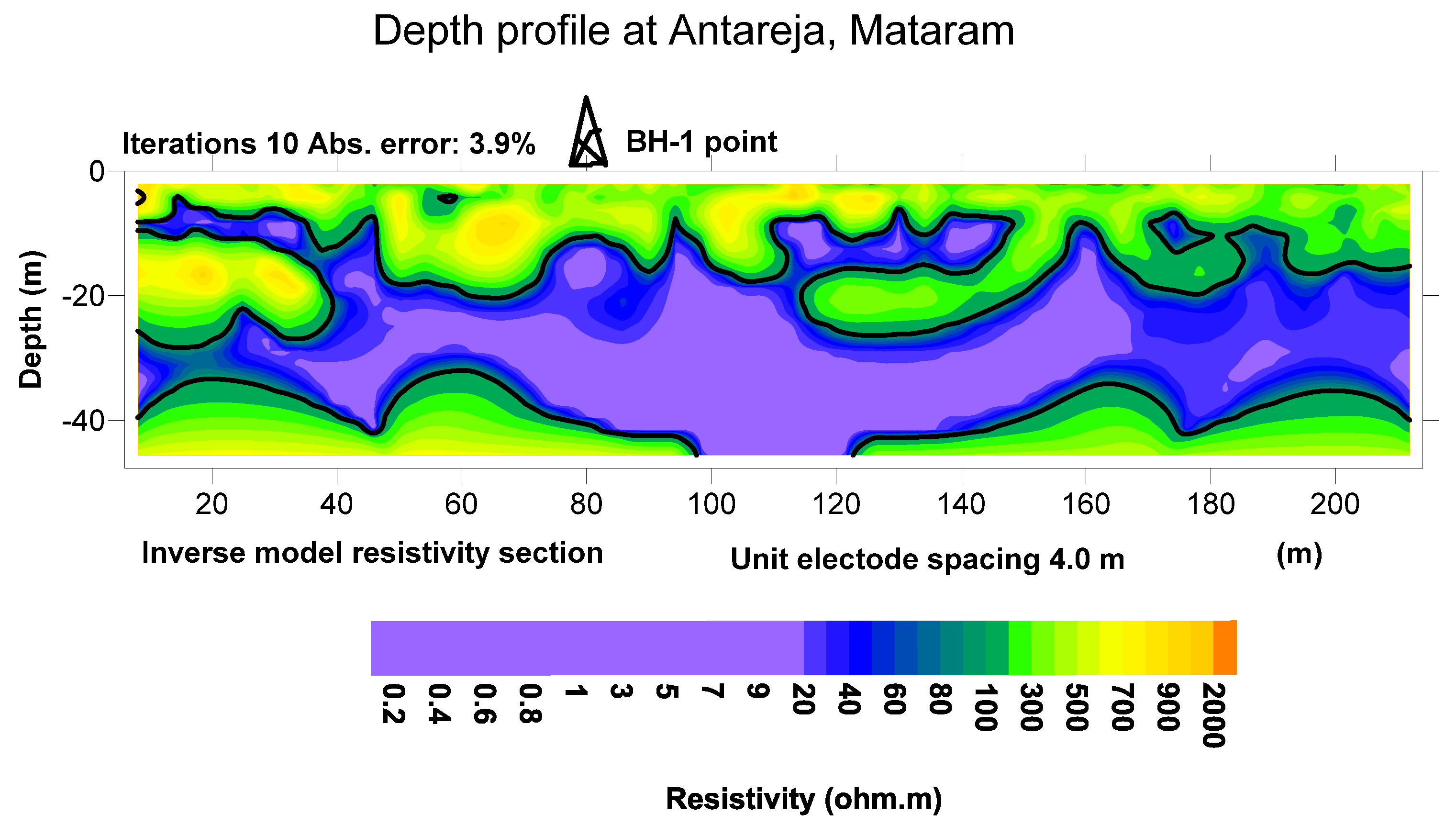
The first section of the 2D resistivity was Antareja crossroad in Mataram (Figure 7). This measurement site was the largest alluvial area with an average altitude of 15–16 m a.s.l. The 2D trajectory mapping was performed with electrodes spaced 4 m and 220 m long track to the North-South direction. The results of 2D inversion (Figure 7) had a wide range of resistivity values from 0.2 to 2000 Ohm.m with an error rate of 3.9%. The results were validated by drilling samples (Table 3). Drilling at this location was taken at 80 m from the starting point of the track at a depth of 21 m from the surface.

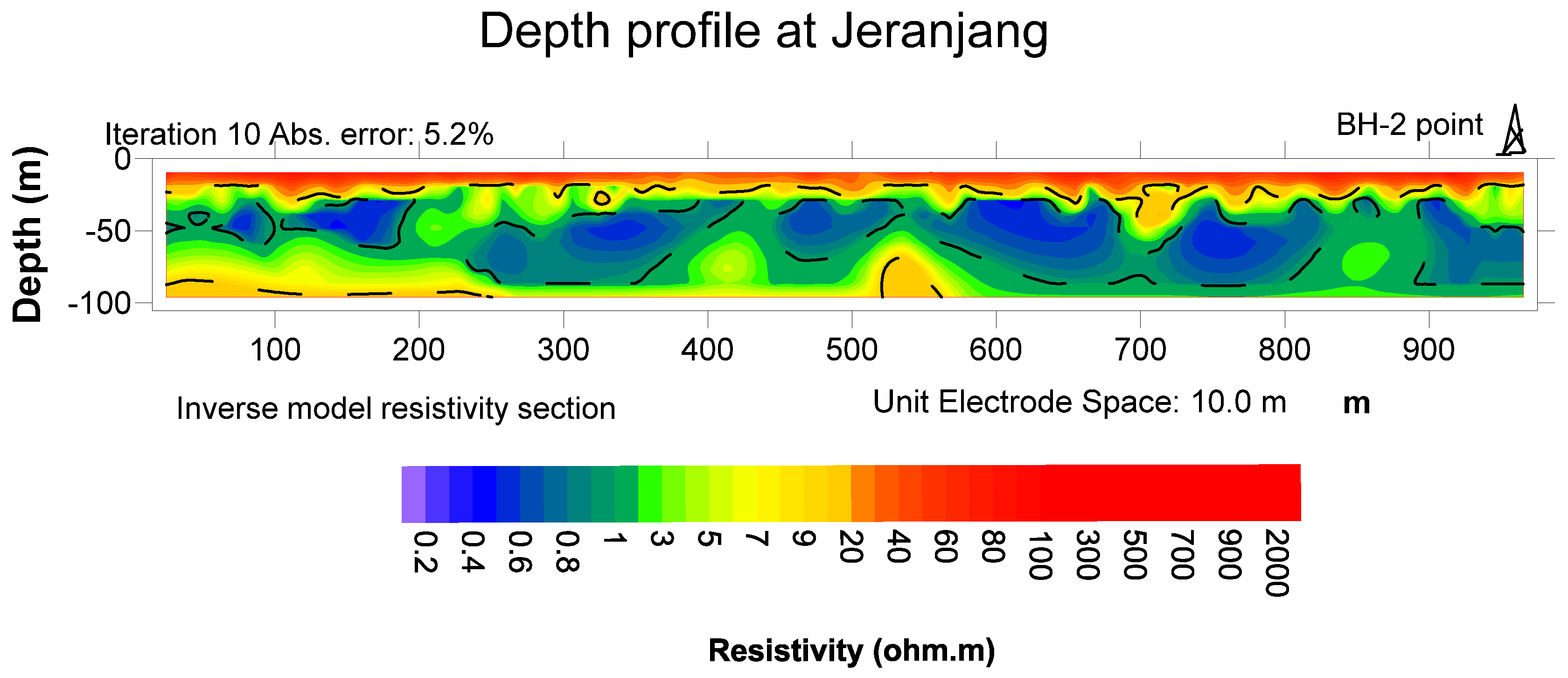
Another 2D mapping was performed in Jeranjang, West Lombok (Figure 8). The location was close to the Jeranjang beach. Data acquisition’s trajectory was directed perpendicularly toward the beach with the electrode spacing of 10 m and a total length of the trajectory of 970 m. Results of mapping 2D inversion (Figure 8) at this location had a wide range of resistivity values of 0.2–2000 Ohm.m with error 5.2%. In this area, 1020 m was drilled in a position with a depth of 10 m. Drilling results and each lithologic log are shown in Table 4.

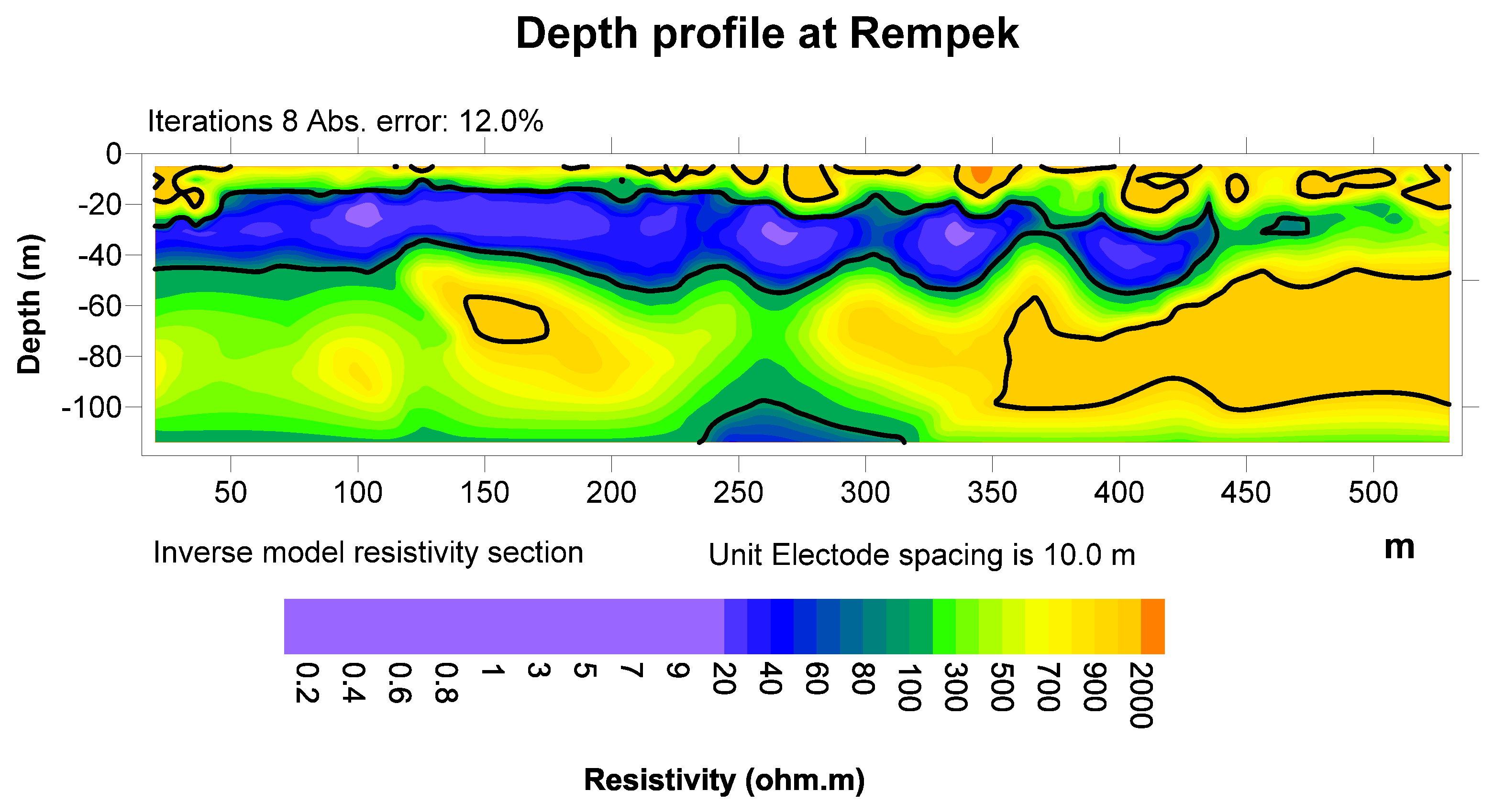
2D mapping was carried out well in some upland areas (>600 m a.s.l.) for example on Batu Ginjang-Rempek (≥900 m a.s.l.) Northwest of Mount Rinjani. This area is quite flat and wide. The data acquisition at this location were: two lines spaced 2.5 m and 4 lines spaced 10 m. Tracks 137.5 m minimum and maximum 1390 m. 2D geoelectric cross-section (Figure 9) is one of the inversion results at this location, with error 12.0%. Resistivity values ranging from 0.2–2000 Ohm.m and a maximum depth of 119 m were the maximum depth of investigation detected. Furthermore, the interpretation of the results of the mapping of 2D inversion is described as follows.

The 2D resistivity’s cross-section in Figure 7 was grouped into three layers. The top layer has resistivity values ranging (150–2000) Ohm.m with an average thickness of 13 m. The first layer was composed of rocks: clay, sand, gravel, coarse grains of pumice stone, mud, black sand and smooth (see Table 3 and Figure 10a), alternately until a depth of 28 m. The second layer with resistivity values from (0.2–150) Ohm.m defined as fine sand, black mud and at a depth of (7–13) m. The third layer having resistivity values: (150–2000) Ohm.m, defined as silt and fine sand saturated with water. This lithology filled the layer to a depth of 47.0 m and was interpreted as paleo-topography. Paleo-topography is the topography of area before the massive eruption of Mount Samalas. High resistivity values (≥150 Ohm.m) was found in the third layer at a depth of 47 m. As elsewhere, this layer was interpreted as the bedrock.

The 2D cross-section’s resistivity in Figure 8 was interpreted as follows: the first layer has a resistance value from (20–2000) Ohm.m with an average thickness of 17.0 m. Based on the drilling data, this layer was filled with clay, sand, pumice granules, fine sand, silt and coarse pumice stone, filling depth of (0–17) m. The second layer had a resistivity value of (0.2–20) Ohm.m. This low resistivity values occupied a depth of (17–27.9) m. The final layer with the depth of 81.9 m and a value of resistivity more than (1.5–20) Ohm.m. The same thing in Figure 9, with a high resistivity value: (150–2000) Ohm.m, was located on the surface to a depth of 17 m and was defined as a layer of volcanic deposits. Second, the value of resistivity: (0.2–150) Ohm.m with a thickness of 29 m. The third layer had a high resistivity of (150–2000) Ohm.m with the depth of 45 m. The second and third layers were treated respectively as paleo-topography and bedrock. The phenomenon of high resistivity values in the first and third layers also occurred in 35 other cross-sectional resistivities. The first layer was interpreted as a layer of volcanic deposits and the third layer as the bedrock. Low resistivity values in the second layer were interpreted as paleo-topography.

4. Discussion

Inversion models from 24 VES which cross the island of Lombok (Figure 1), composed of type curves [20,21]: type HKH, 25%, KHKQ, 12.5%, Type HK and KQH respectively 8.3% and 11 other types respectively 4.2%. The VES inversion model in Figure 3 and Figure 5, both of are, showing the resistivity values of level bedding with high, medium and low, as the characteristics of the sediment. The data of VES model in Figure 3 was acquired from the slopes, and in Figure 7 was acquired from alluvial areas. Both data VES models were very helpful in mapping the layer of volcanic deposits with great details in the vertical direction. A layer of volcanic deposits as described above, particularly a layer of pumice in Figure 4, had a resistivity value of 700 Ohm.m, while pumice in Figure 6 reflects the value of resistivity of 180 Ohm.m. The values’ comparison was much smaller than that in the slope areas.

This condition could be explained because of the physical characteristics of pumice itself and environmental conditions of deposition. Resistivity values are influenced by saturation, alteration and porosity variation together with mineralogical compositions. Pumice, in both slopes and alluvial areas, has the same various porosity and composition because it was acquired simultaneously in one event time and the same source, Mount Salamas. Pumice in both areas also was altered. Pumice stone in sloping areas possesses physical characteristics: over the shaft, the pores are filled with air, more rugged, shape and geometry various and waterless as we see in Table 1 and Table 2. These characteristics are contributed to increasing resistivity value. Meanwhile, the physical characteristics of pumice in alluvial areas (Figure 6) was more compact and saturated where its pores were filled with clay or water. Both clay and water contribute to reducing resistivity value.

Secondly, the drier the depositional environment was, the more homogeneous and shaft it would be. They were the factors that caused the higher value of resistivity of pumice on the higher slopes. On the contrary, in alluvial depositional was relatively more humid and heterogeneous, as we see in Table 3 and Table 4, characteristics lithologic of the sample borehole in Antareja, Mataram (BH-1) and Jeranjang, West Lombok (BH-2). The borehole data was used to constrain models. Such is the case with alteration, where the rock started having reduced resistivity value treat. The same thing, if rocks contain water or clay.

The outcrops of volcanic deposits were at Krumut beach (Figure 6), particularly the layer of pumice in the second and fourth layers. The second layer had different physical characteristics compared with the fourth layer. The differences in these characteristics showed there was an eruption event in two different phases. The first stage, pumice which was located on the fourth layer had the following characteristics: oval, reddish, size of (106.25 × 78.65) mm, porous, and could be destroyed by finger. The thickness of the layer was 0.5 m and was located at a depth of 1.80 m. The average resistivity value was 276.40 Ohm.m. At the second stage, characteristics of pumice layers of oval, rough, porous, brown, very pivot and fresh. These outcrops were located on the second layer with an average thickness of 0.30 m and resistivity value of 188.90 Ohm.m. Other similar outcrops were found in the northwest of Mount Rinjani, in Tebing beach (OC-4), Lokok Meang (OC-3), Lokok Piko and Anyar beach.

The second type of outcrops, which had different characteristics from the previous outcrops, was located at Medana, Samba, Sanjajak, Batu Ginjang, and Sembalun. The outcrops generally became the topographic coat and closer to the source. Outcrops came in the form of clay, pumice, and sand. The pumice’s physical characteristics: oval, fresh, and sorrel. The third kind of outcrops was found in the southern part of Mount Rinjani at Benang Kelambu, Benang Stokel, South Batukliang, and Barabali-Kopang as well as in the Southwest of Penimbung to Bukit Tinggi. To the next, we were discussion the result of ERT.

The 2D inversion models indicated three unit layers with high resistivity contrast as shown in Figure 7, Figure 8 and Figure 9. The Figure 7 and Figure 9 showed three units of the layer where a layer of volcanic deposits located in the uppermost layer with high resistivity values more than 150 Ohm.m, while in Figure 8 the uppermost layer has high resistivity of more than 20 Ohm.m. Meanwhile, low resistivity (<150 Ohm.m) in Antareja and Rempek while in the Jeranjang, the resistivity less than 20 Ohm.m. The second layer, we interpreted as the Paleo-topography. The third layer is a layer of bedrock with high resistivity values (20–2000) Ohm.m.

For the 2D geo-electric cross-section, the inversion results show the same layering pattern, characterized by a contrasting resistivity pattern. The changing pattern in the value of resistivity was in sharp contrast to the vertical direction, i.e., from a high value to low resistivity value. Then followed by a change from a low value to high value again. In contrast to the variation of the horizontal direction and isopach thickness, the resistivity almost had the same value. High resistivity values (>150 Ohm.m) in the uppermost layer showed the volcanic deposits. Volcanic deposits consisted of clay, sand, pumice, ash, and PDCs. Low resistivity values (<150 Ohm.m) in the second layer was a reflection of the fine sand and black mud. The second layer was interpreted as Paleo-topography that existed before the eruption in 1257 AD. High resistivity values (20–2000) Ohm.m in the third layer was interpreted as bedrock consisting of sandstone and mudstone. To the next, we discussed about the influence of geomorphology, topography, and distance to isopach volcanic deposits. To answer this question, here is the isopach map analysis: an analysis of isopach across the source area and the function of distance from the source is shown in Figure 11 and Figure 12 below.

The isopach mapping of volcanic deposits (Figure 11) was constructed from the interpretation of VES and 2D geo-electric mapping. Isopach map was divided into three main areas: Mataram, Tanjung, and Korleko. Thin isopach (<25 m) generally occupied an area of alluvial deposits, such as Mataram, Tanjung, and Korleko. Instead, thick isopach (>25 m) was found on the slopes, for example in Sedau, at Tebing beach, Luk, Rempek, and Mamben. The next thing is how influential the distance to the isopach value was?

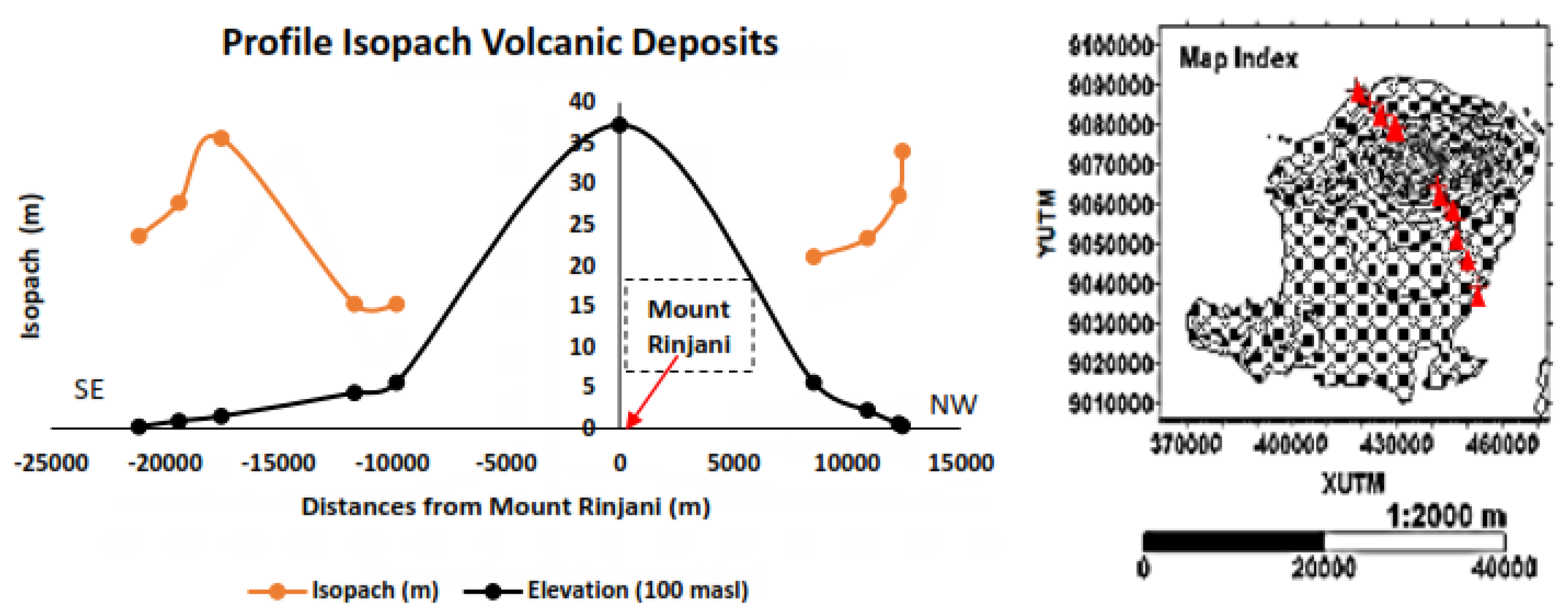
The isopach profile of volcanic deposits that crosses the island of Lombok was shown in Figure 10. The profile was obtained from the inversion of 24 points of VES and 2 site outcrops in the direction of Southeast-Northwest. Isopach seemed not linear from the source (zero distance) to the beach in both crossed directions. Isopach from a distance of 21 to 31 km to the North-West and in the 15 to 21 km to the southeast, both rose sharply. Conversely, at a distance of 21 to 28 km, the depletion of isopach was too steep. The maximum isopach in Southeastern was found in Mamben at a distance of 21.17 km, and in the Northwest that was in Tebing beach at a distance of 31 km.

The geomorphological condition of measurement location in the southeast of Karang Baru until Kembang Kerang was quite steep (see Figure 10c). Furthermore, from Kembang Kerang to Krumut Beach, the geomorphological conditions tend to be ramps and flat areas. Thick outcrops (± 20 m) were found in the area of the ramps precisely in Ladon-Mamben Lauq. While the geomorphology at Northwestern of Mount Rinjani from Sanjajak to Tebing beach was a fairly steep. A thick PDCs was found at northwestern like: in Lokok Meang_Luk (OC-3) is 20 m and Tebing Beach (OC-4) is 34 m (Figure 1, Figure 11 and Figure 13).

The thick outcrops above were generally dominated by PDCs, both in the East and in the West Sea. PDCs layers consisted of clay, pumice stone, and alternated with layers of sand and volcanic ash and inserts of ignimbrite. These thick isopachs were located at specific points. It showed that the topography did not affect the value of the isopach (see Figure 10). In the next paragraph, we discuss the affects of distance sites to the isopach value.

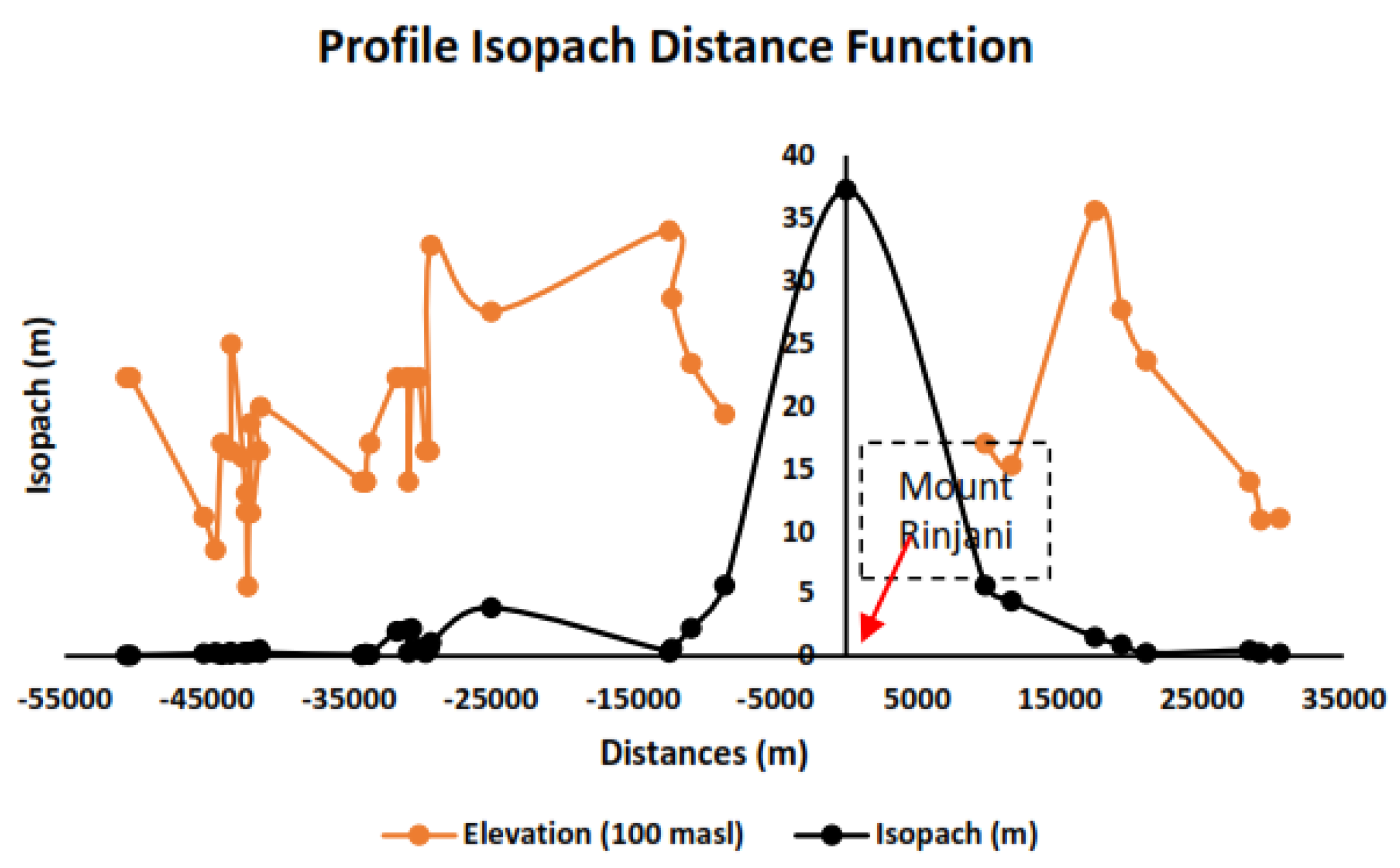
The profile of isopach geomorphology function (Figure 12), which are the distance measured from sites to the source, is shown in Figure 1. The distance was measured based on the position of the measuring point from Mount Rinjani, as the source. The consecutive point of measurement: 24 VES, two outcrops, and 35 geoelectric 2D mapping. The note is that isopach rose sharply to the NW from a distance of 21.20–30.83 km, and to the east SE at a distance of 14.76 to 21.17 km. A maximum isopach (34 m) occurred at a distance of 30.83 km to NW, precisely at the Tebing Beach, and isopach 35.60 m at a distance of 21.17 km to the SE, especially in Mamben. Isopach was sharply reduced from a distance of 30.83 to 50.36 km to the NW and at a distance of 21.17 to 30.51 km (Figure 12) in the SE Mount Rinjani and Mount Samalas.

Isopach deployment directions showed the dominant effect of the wind at the time of eruption [1]. The isopach of volcanic deposits on slopes was greater than in the alluvial areas. The sufficient distance to the source became the factors that affect the value of isopach of volcanic deposits. However, the effect of isopach value was not very significant on the geomorphology for the fallout of deposition.

The field observations indicated that the main volcanic sediment, which consisted of precipitation of the fall, stream sediment and PDCs sediment as described by [1]. The precipitated fallouts spread widely and evenly throughout the Lombok. Debris deposits generally cover (coat) topography, parallel layers (beds), good order, both relegated, a grain size of multi-mode, and widespread and evenly, as described by [14]. The fall deposition was interspersed with sporadic wave (surge) pyroclastic, particularly in the area of alluvial re-deposition. The type of rock layers that made up the beds volcanic deposits included: clay, gravel, pumice sand, sand, pumice granules rough, silt and black fine sand, as described by [15].

The VES data provided important information about isopach and paleo-topography. The applications of VES were very effective in mapping the volcanic deposits. The same thing had been performed by [4,20]. The 2D resistivity of geoelectric mapping was useful in distinguishing layers of volcanic deposits and the essential sediments, as had been conducted by [8,9,20].

The results of this study were the first geophysical research in Lombok Island particularly the research associated with volcanic deposits of Mount Samalas. The application of geoelectrical method was one of the geophysical innovations especially for isopach mapping of volcanic deposits on the slope areas which were difficult-to-access areas. However, this research data was still lacking, especially to the South, Northeast, and Southwest as well as in the area of Segara Anak caldera. Preferably in the same study, the geoelectrical method, combined with another geophysical method, such as seismic refraction, seismic reflection and Multi Channel Analysis of Surface Waves (MASW). Second, further study of this research will be the analysis of the eruption’s dynamics of Mount Samalas in the past.

5. Conclusions

We used a combination of geophysical methods, field surveys and drilling in order to map the isopach of volcanic deposits distribution, both in the alluvial region and in the sloping region. The border of isopach of volcanic deposits and paleo-topography was characterized by the contrast of high resistivity value. Isopach resistivity values on the slopes were generally higher than in the alluvial areas. The average value of the resistivity of volcanic deposits in the alluvial areas: (20–958) Ohm.m and on the slope areas (150–1936) Ohm.m. Isopach volcanic research areas were ranging from (6–36) m. Bedding patterns and isopach had similar characteristics to other sites, both in vertical and horizontal directions. The value of the isopach volcanic deposits on the slopes of the area generally higher (>25 m) compared with the alluvial area (<25 m). Both the geomorphology and the distance seems not linear on the increase or decrease in the value of isopach. Isopach thick occurs at a certain distance and area. Generally, increased isopach occurred between a distance of 14 km and 31 km from the source. In the future, there will be an analysis of the dynamics and ballistic simulation of the eruption of Mount Samalas 1257 AD, for prediction and mitigations in the future. In the future, there will be an analysis of the dynamics and simulation of the ballistic eruption Samalas 1257 AD and image subsurface of the Samalas mount. This analysis useful for prediction dynamics of eruptions, and disaster mitigation.

References

1. Lavigne, F.; Degeai, J.-P.; Komorowski, J.-C.; Guillet, S.; Robert, V.; Lahite, P.; Oppenheimer, C.; Stofflel, M.; Vidal, C.M.; Surono; et al. Source of the Great A.D.1257 Mystery Eruption Unveiled, Samalas Volcano, Rinjani Volcanic Complex, Indonesia. PNAS 2013, 110. [Google Scholar] [CrossRef] [PubMed]
2. Bonadonna, C.; Phillips, J.C. Sedimentation from strong volcanic plumes. J. Geophys. Res. 2003, 108, 2340. [Google Scholar] [CrossRef]
3. Reynolds, J.M. An Introduction to Applied Environmental Geophysics; John Wiley & Sons Ltd.: West Sussex, UK, 1997. [Google Scholar]
4. Batayneh, A.T. Application of geoelectric methods on paleoenvironments of the Qa’el-Jufr Lake, southeastern Jordan Plateau. J. King Saud Univ. Sci. 2011, 23, 381–388. [Google Scholar] [CrossRef]
5. De Vita, P.; Agrello, D.; Ambrosino, F. Landslide susceptibility assessment in ash-fall pyroclastic deposits surrounding Mount Somma-Vesuvius: Application of geophysical surveys for soil thickness mapping. J. Appl. Geophys. 2006, 59, 126–139. [Google Scholar] [CrossRef]
6. De la Vega, M.; Lopez, E.; Osella, A.; Rovere, E.I.; Violante, R.A. Quaternary volcanic sedimentary sequences and evolution of the Llancanelo Lake region (Southern Mendoza, Western Argentina) evidenced from geoelectric methods. J. South Am. Earth Sci. 2012, 40, 116–128. [Google Scholar] [CrossRef]
7. Urrutia Fucugauchi, J.; Trigo-Huesca, A.; Téllez García, E.; Pérez Cruz, L.; Méndez Rivero, F. Volcano-sedimentary stratigraphy in the Valsequillo Basin, Central Mexico inferred from electrical resistivity soundings. Geofisica Int. 2014, 53, 87–94. [Google Scholar] [CrossRef]
8. Saribudak, M.; Caran, C. Resistivity, Magnetic Data Delineate Volcanic Tuff in Travis County, Tex; Environmental Geophysics Associates: Austin, TX, USA, 2015. [Google Scholar]
9. Violante, R.; Osella, A.; de la Vega, M.; Rovere, E.; Osterrieth, M. Paleo-environmental reconstruction in the western lacustrine plain of Llancanelo Lake, Mendoza, Argentina. J. South Am. Earth Sci. 2010, 29, 650–664. [Google Scholar] [CrossRef]
10. Wacana, L. Babad-Lombok; Departemen Pendidikan dan Kebudayaan Proyek Penerbitan Buku Bacaan Sastra Indonesia dan Daerah: Jakarta, Indonesia, 1979; p. 66. Available online: https://openlibrary.org/books/OL2703706M/Babad_Lombok (Accessed on 3 July 2017).
11. Smithsonian Institution. Global Volcanism Program. Available online: http://volcano.si.edu/ (Accessed on 13 July 2017).
12. Asnawir, N.; Akira, T.; Udibowo; Djedi, S.W.; Hutasoit, L.M. Rinjani and Paropok Volcanics as a Heat Sources of Geothermal Prospects from Eastern Lombok, Indonesia. In Proceedings of the World Geothermal Congress, Bali, Indonesia, 25–29 April 2010. [Google Scholar]
13. Vidal, C.M.; Pratomo, I.; Carazzo, G.; Komorowski, J.C.; Kartadinata, N.; Lavigne, F.; Métrich, N.; Prambada, O.; Rodysill, J.; Michel, A.; et al. Dynamics of the major plinian eruption of Samalas in 1257 A.D. (Lombok, Indonesia). Bull. VolIcanol. 2015, 73. [Google Scholar] [CrossRef]
14. Maeno, F.; Nakada, S.; Nagai, M.; Kozono, T. Ballistic ejecta and eruption condition of the vulcanian explosion of Shinmoedake volcano, Kyushu, Japan on 1 February 2011. Earth Planets Space 2013, 65, 609–621. [Google Scholar] [CrossRef]
15. Mangga, S.A.; Atmawinata, S.; Hermanto, B.; Setyonugroho, B.; Amin, T.C. Geological Map of the Lombok Sheet, West Nusa Tenggara; Departemen Pendidikan dan Kebudayaan Proyek Penerbitan Buku Bacaan Sastra Indonesia dan Daerah: Jakarta, Indonesia, 1994. [Google Scholar]
16. Loke, M.H.; Chambers, J.E.; Rucker, D.F.; Kuras, O.; Wilkinson, P.B. Recent developments in the direct-current geoelectrical imaging method. J. Appl. Geophys. 2013, 95, 135–156. [Google Scholar] [CrossRef]
17. Chitea, F.; Ioane, D.; Airinei, I.; Serban, A.; Dorobantu, A. Geoelectrical Methods Applied for Prospecting an area with geothermal potential. In Proceedings of the 14th SGEM GeoConference on Science and Technologies in Geology, Exploration and Mining, Sofia, Bulgaria, 17–26 June 2015; SGEM: Sofia, Bulgaria, 2014. [Google Scholar]
18. Bahkaly, I.M.; Jallouli, C.; El-Waheidi, M.M.; Batayneh, A.T. Assessment of shallow aquifer salinity in the Aqaba Coastal plain using ERT method: a case study of Maqnah region, northwestern Saudi Arabia. Environ. Earth Sci. 2015, 74, 2105–2114. [Google Scholar] [CrossRef]
19. Kumar, N.; Rao, R.; Naganjaneyulu, K. Electrical resistivity imaging (ERI) using multielectrodes for studying subsurface formations in Cauvery plains. Adv. App. Sci. Res. 2015, 6, 47–53. [Google Scholar]
20. Zohdy, A.A. Use of Dar Zarrouk Curves in the Interpretation of Vertical Electrical Sounding Data; No. 1331; USGS: Washington, DC, USA, 1974.
21. La Delfa, S.; Camuti, M.G.; Patané, G. A multi disciplinarity study of the volcanic deposit named “Chiancone”, inland and offshore, in the frame of the evolution of volcanism in the Etna area. Phys. Earth Planet. Inter. 2011. [Google Scholar] [CrossRef]
22. Gyulai, Á.; Ormos, T.; Dobroka, M. A quick 2-D geoelectric inversion method using series expansion. J. Appl. Geophys. 2010, 72, 232–241. [Google Scholar] [CrossRef]
23. USGS. Lithclass polygon colors. Available online: http://mrdata.usgs.gov/catalog/lithclass-color.php (accessed on 27 May 2017).
24. Van Dam, R.L. Landform characterization using geophysics—Recent advances, applications, and emerging tools. Geomorphology 2012, 137, 57–73. [Google Scholar] [CrossRef]
25. Loke, M.H. Tutorial: 2-D and 3-D Electrical Imaging Surveys. Available online: http://personales.upv.es/jpadin/coursenotes.pdf (accessed on 3 July 2017).
26. Constable, S.C.; Parker, R.L.; Constable, C.G. Occam’s inversion: A practical algorithm for generating smooth models from electromagnetic sounding data. Geophysics 1987, 52, 289–300. [Google Scholar] [CrossRef]
Figure 1. Geological map of Lombok Island and the study location (modified after [15]). Mount Samalas and Mount Rinjani, both indicated with green fill triangle, as a source of Sediment volcanic and created Segara Anak lake. Location of geoelectrical measurement: VES is indicated with the red triangle and the ERT section are indicated with red circles The Borehole is indicated with the white flag and the Outcrops is indicated with the squares.
Geosciences 07 00067 g001
Figure 2. (a) Wenner-Schlumber array and (b) Dipole-dipole array.
Geosciences 07 00067 g002
Figure 3. The Profile of the VES data inversion results (all types HKH) and outcrops in Samba (OC2), Northwest (417,258, 9,081,645) UTM of Mount Rinjani. S1, S2, and S3 are sounding numbers of VES. The outcrop (photographed by the authors, 2015) layers from the surface were: dry clay with a pumice stone inserts, with the thickness of 0.80 m, the second rough pumice stones with sand inserts (interpretation of resistivity values and layers’ thickness, in the text).
Geosciences 07 00067 g003
Figure 4. (a) Depth profile of the resistivity, and (b) resistivity logs (its color is based on Lithclass polygon colors (23)); and (c) lithologic logs at Samba. D1, D2, D3: depth soundings S1, S2, S3 in Figure 2. Dave: average depth profiles D1, D2, D3. The S1 location is (417,258; 9,081,645) UTM and its elevation is 224 m a.s.l. Spacing S1 to S2 is 30 m and to S3 is 60 m and elevation of S2 is 232 m a.s.l. and S3 219 m a.s.l. The depth of zero means situated at ground level. The outcrop (c) consists of dried clay, pumice, and sand mixed pumice stone.
Geosciences 07 00067 g004
Figure 5. (a) Five VES resistivity profiles (types: AKHQ, AKQQ, KQ, AKHKQ and AKHKQ) [20,21,22]. were taken on above outcrop; (b) Outcrop of volcanic deposits of Krumut Beach (OC-1), where the acquisition of VES was executed. S1 to S5: sounding point numbers. Rock type’s layers: clay, coarse pumice, alternating sand and pumice, weathered pumice and sand inserts ignimbrites (see depth profile and Log resistivity in Figure 6 and text for more info).
Geosciences 07 00067 g005
Figure 6. (a) VES Depth Profile of 5 soundings in Krumut beach. D1 to D5: Soundings depths, S1 to S5 (Figure 5); Dave: average depth of five soundings; (b) Logs of average resistivity and lithology in Krumut beach [23]; (c) The outcrop (OC-1, see Figure 1). Based on the outcrop, the values of resistivity and thickness of the successive layers of the surface: 127.04, 188.80, 364.80, 364.80, and 276.40 Ohm.m, and: 0.74, 0.73, 0.93, 0.95, and 4.62 m.
Geosciences 07 00067 g006
Figure 7. 2D geo-electrical cross-sections of Antareja Street, Mataram-Lombok (403,754, 9,050,304) UTM (see Figure 1). BH-1: location of the drilling and sediment sampling up to 21 m depth (see Table 3).
Geosciences 07 00067 g007
Figure 8. The 2D geo-electrical cross-section in Jeranjang, West Lombok (398,963, 9,042,313) UTM (see BH-2, on Figure 1). The Well point: the extended point at position 1020 m from the end of the line. It was drilled and samples were taken every meter, to a depth of 10 m of the site (see Table 4 and text).
Geosciences 07 00067 g008
Figure 9. The 2D geo-electric cross-section in Batu Tinjang-Rempek (412,596, 9,080,848) UTM (see Figure 1). The Line length of 550 m, and the electrode spacing of 10 m. Resistivity value ranged from (0.2–2000) Ohm.m. The boundaries between layers could be seen obviously which were characterized by high resistivity contrasts.
Geosciences 07 00067 g009
Figure 10. Isopach mapping of Mountains Samalas sediment, which was built upon the geoelectric observation data. (a) Isopach map in Mataram and its surroundings; (b) the isopach map in the Tanjung region and; (c) the isopach mapping of the Korleko region. The experimental points indicate with red ball for 2D mapping and triangle for VES points, while the Flag indicated Boreholes and the outcrops (OC) indicated with fill rectangles. The Mount Samalas and Mount Rinjani as sources volcanic deposits are indicated in the map index. The 3D contour isopach algorithm was a kriging algorithm with range values: 6–40 m and its interval is 2 m.
Geosciences 07 00067 g010
Figure 11. Sediments isopach profile from Mount Samalas crossed the Lombok Island in the direction of Southeast-Northwest (SE-NW). The red line on isopach profile was the volcanic deposits, and the black line was the topography in 100 MASL. A reference point (zero distance) was the position of Mount Rinjani (441 288, 9,069,599) UTM and 3726 m asl. The minus sign meant next to Southeast and vice versa in the Northwest of Mount Rinjani.
Geosciences 07 00067 g011
Figure 12. The influence of distance from the source toward the isopach thickness. The black line showed the isopach profile and the red line the topography in 100 MASL. The reference point (zero distance) is the position of Mount Rinjani (441 288, 9,069,599) UTM, 3726 masl. The minus sign means the location on the west side of Mount Rinjani. All experiment points (VES and 2D mapping) are indicated in map Figure 1 and Figure 10.
Geosciences 07 00067 g012
Figure 13. (a) Outcrop at Lokok Meang-Luk (OC-3, Figure 1). (b) Outcrop at Tebing Beach (OC-4, Figure 1). Both these outcrops composed of volcanic materials of Mount Samalas 1257 AD. These outcrops consist of volcanic ash, granulated pumice stone, sand, and ignimbrite. For detail, see Table 1 and Table 2 and text.
Geosciences 07 00067 g013