Quantifying Porosity through Automated Image Collection and Batch Image Processing: Case Study of Three Carbonates and an Aragonite Cemented Sandstone

 , ,
, ,
Abstract
:1. Introduction
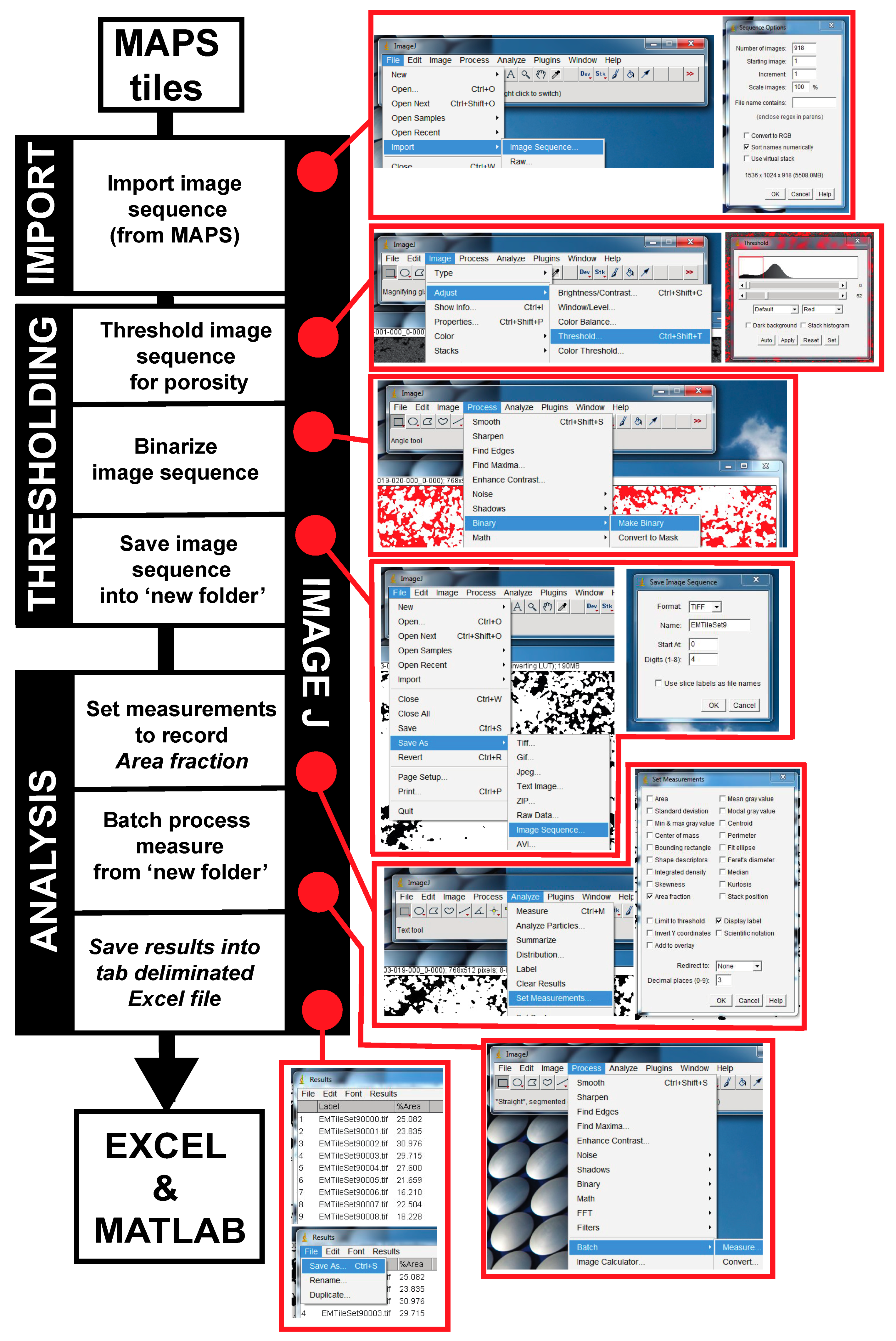
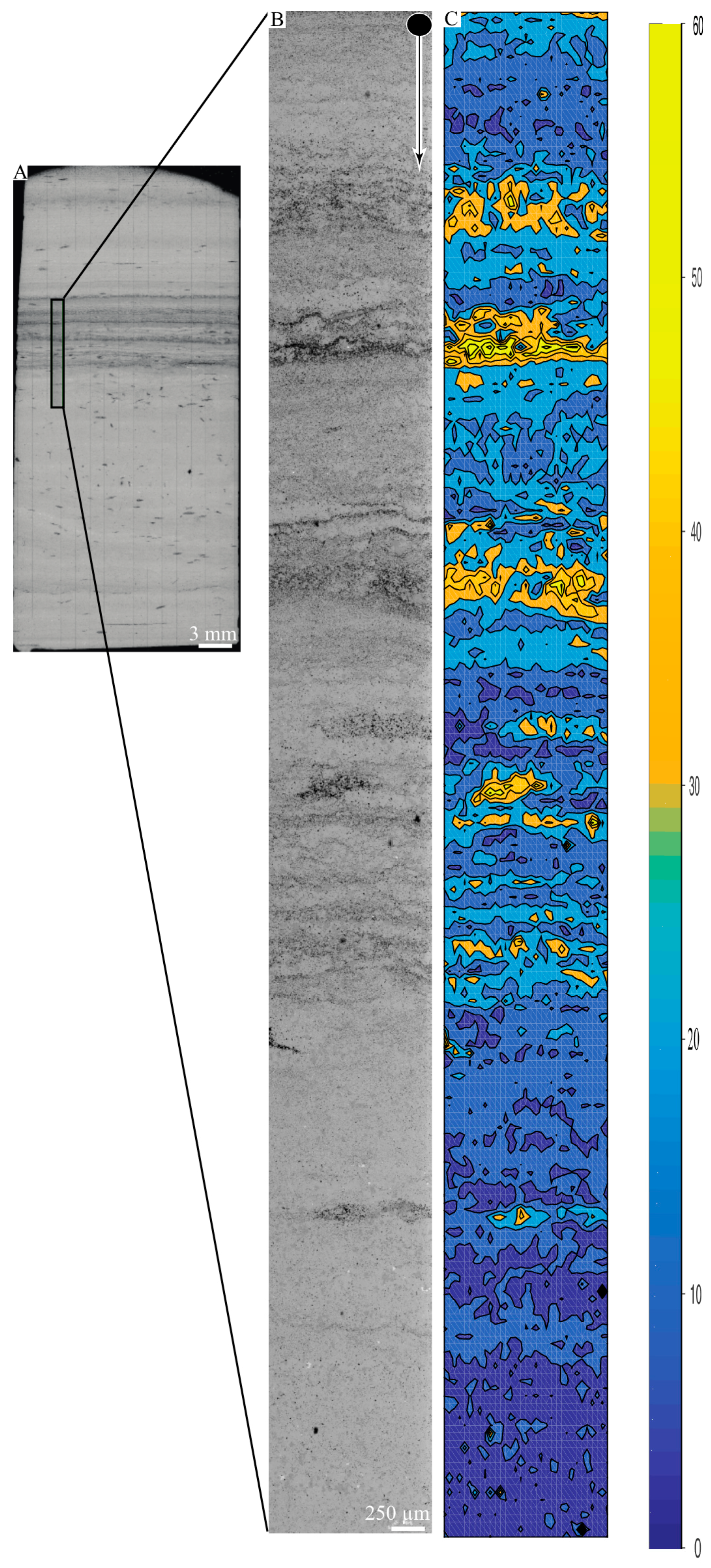
2. Materials and Methods
3. Results
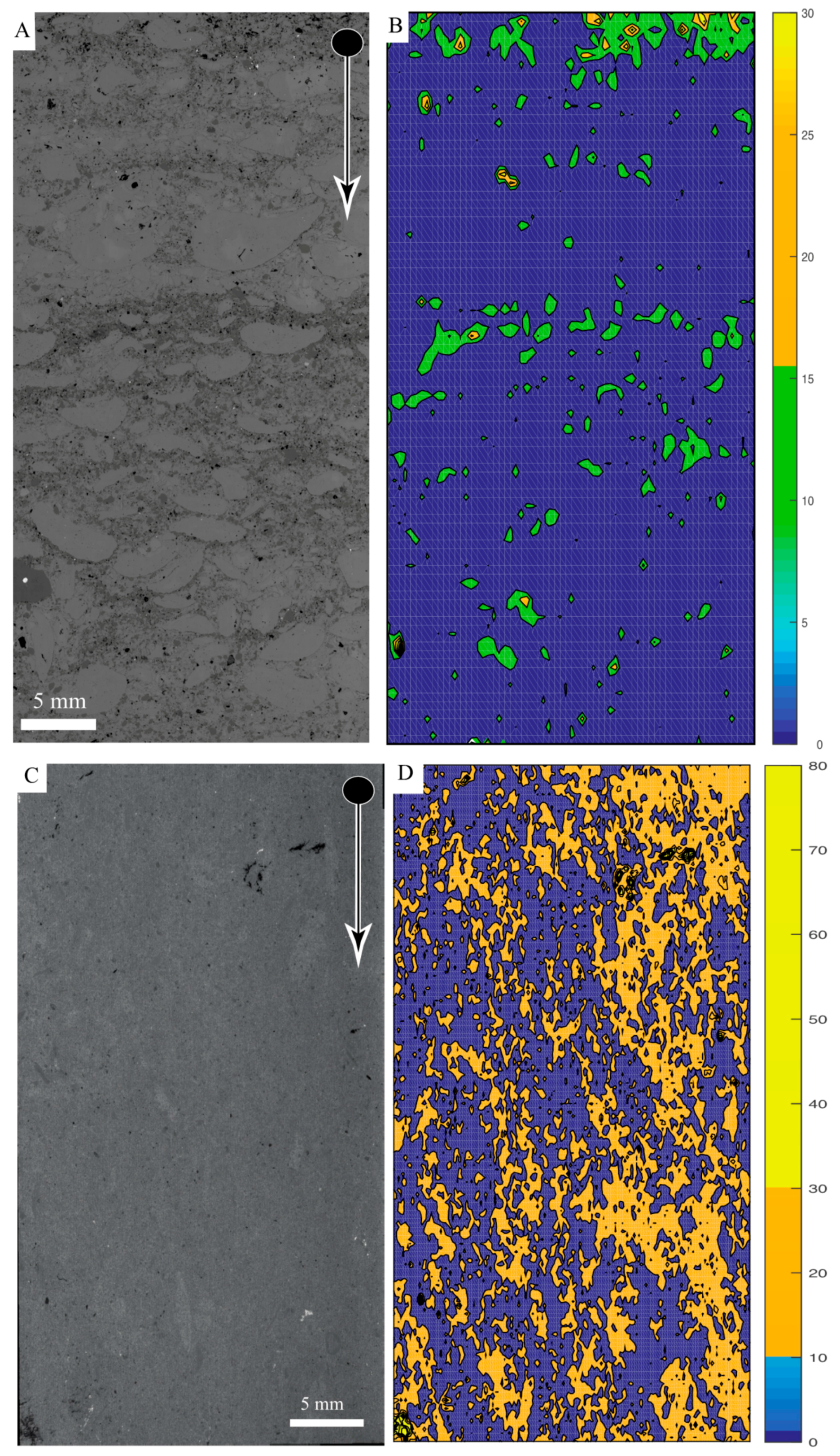
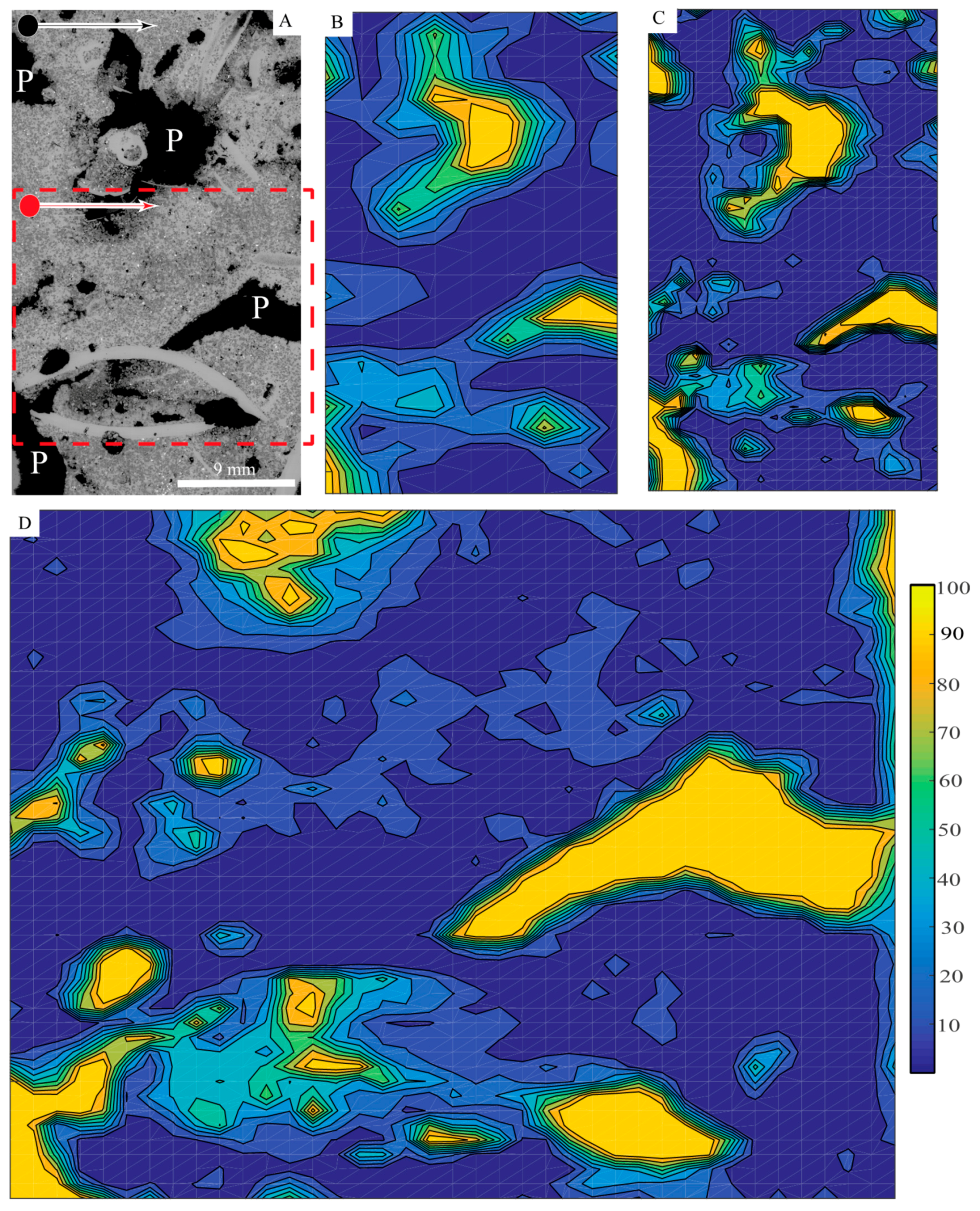
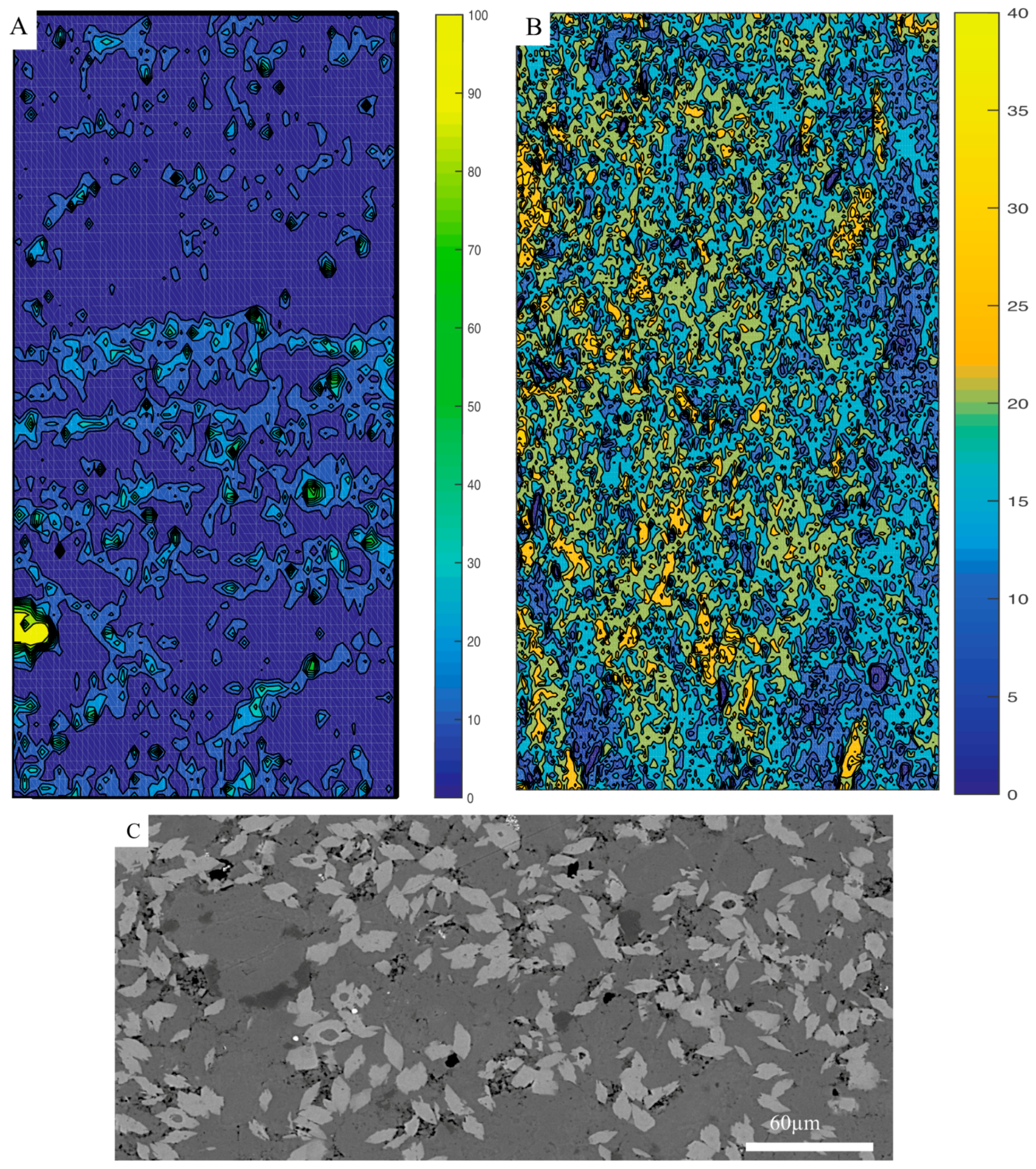
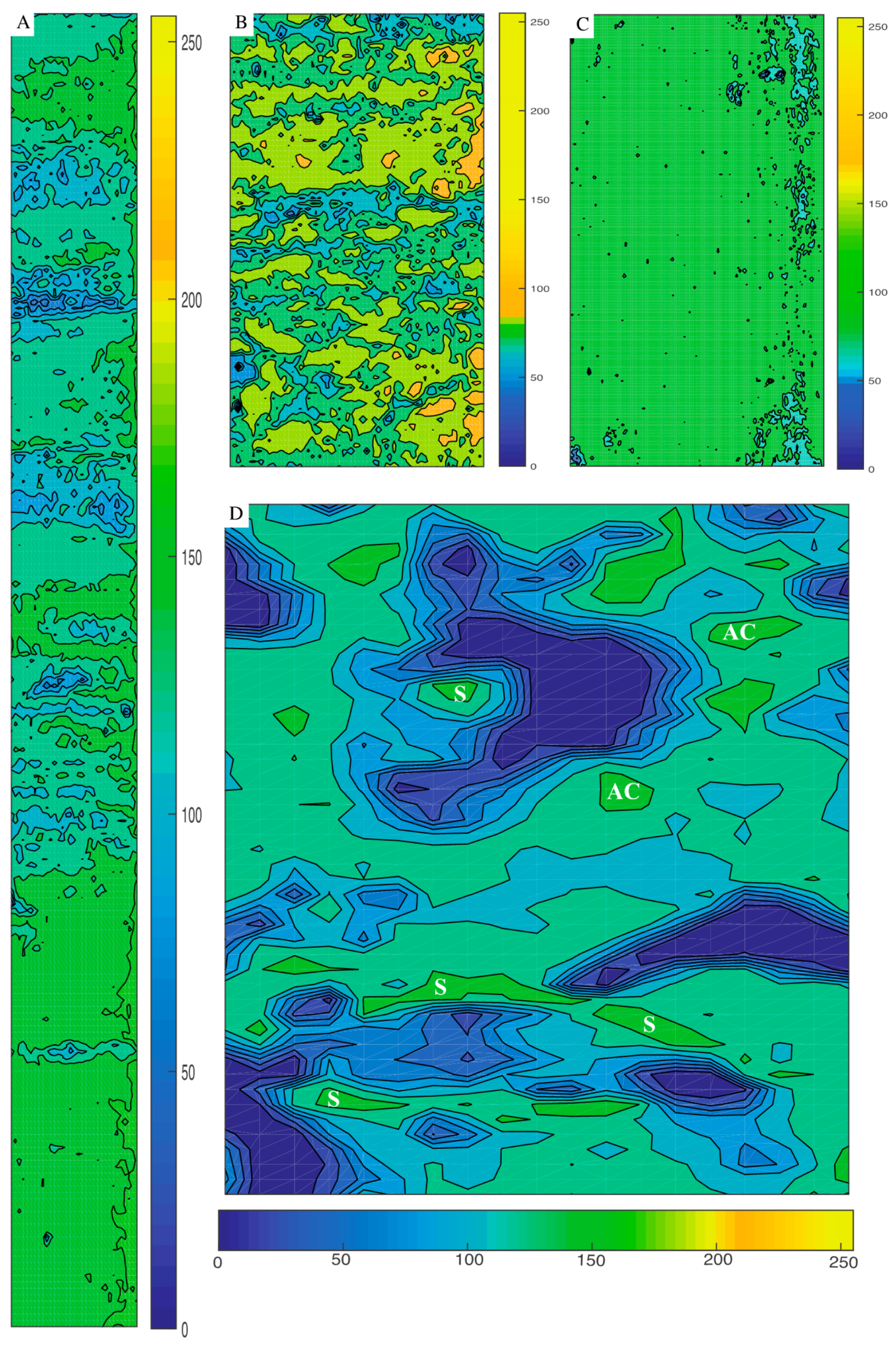
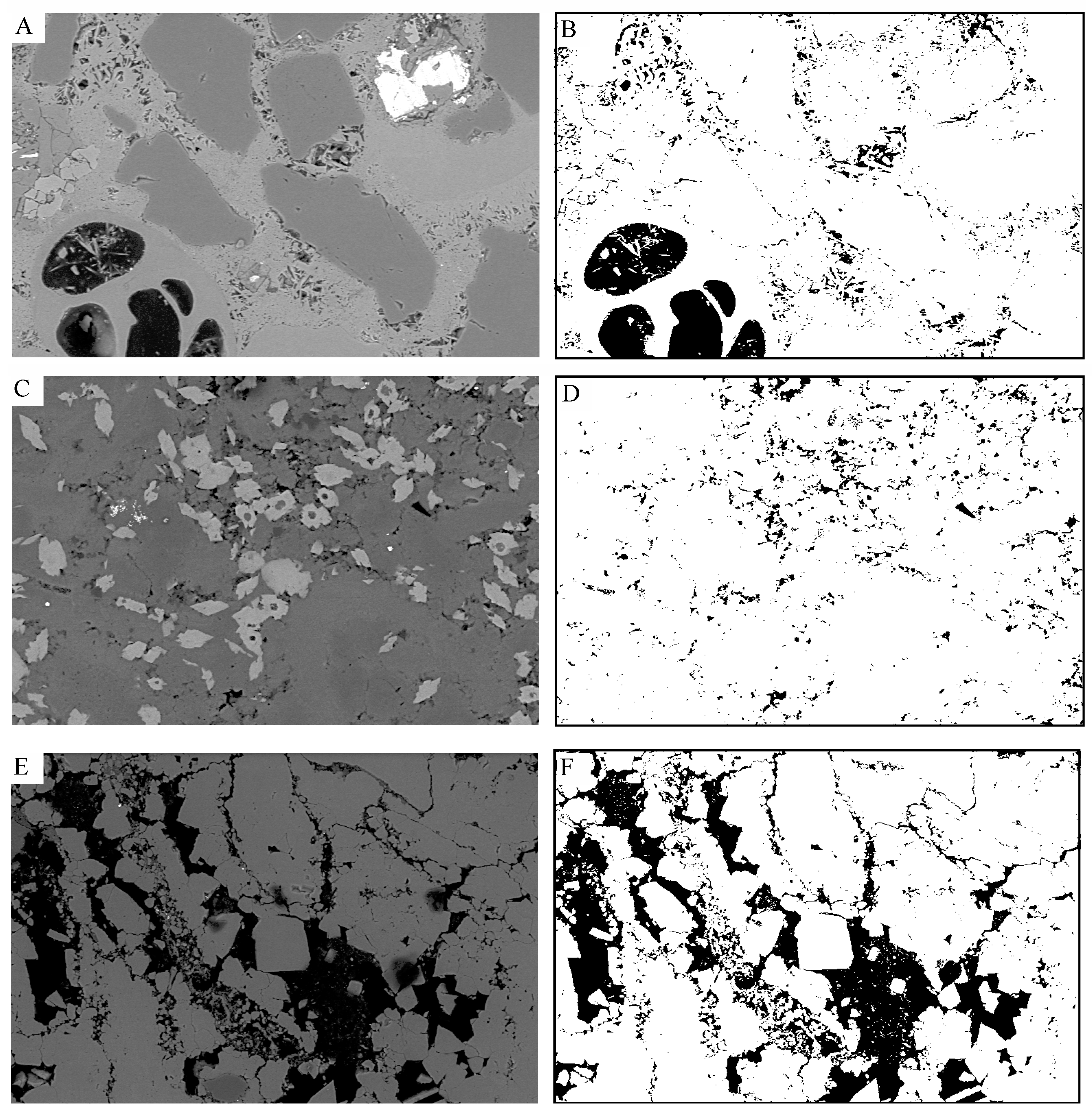
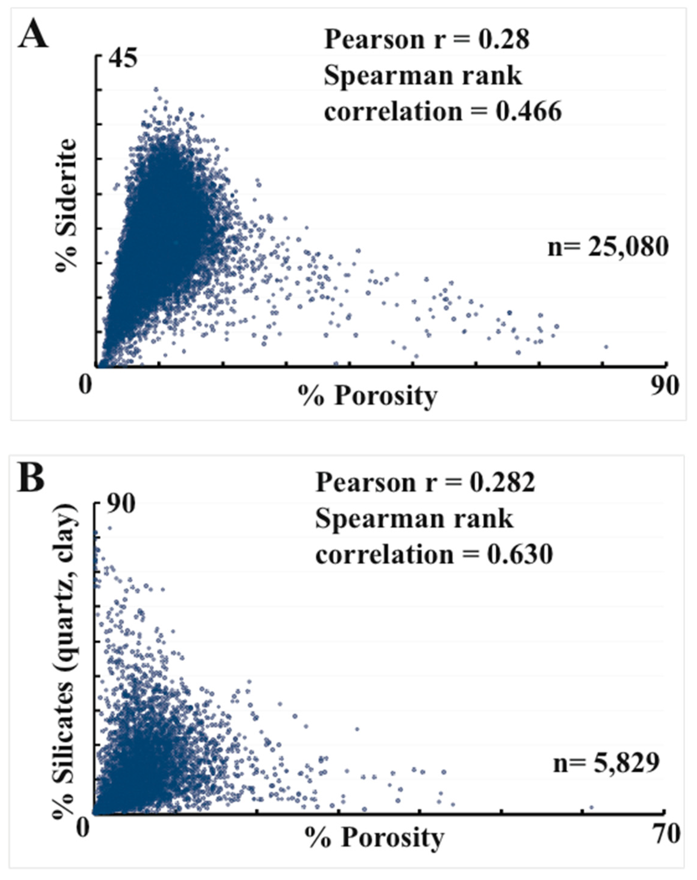
3.1. Porosity Percentage
3.2. Mineral Distribution
3.3. Mean Grayscale
4. Discussion
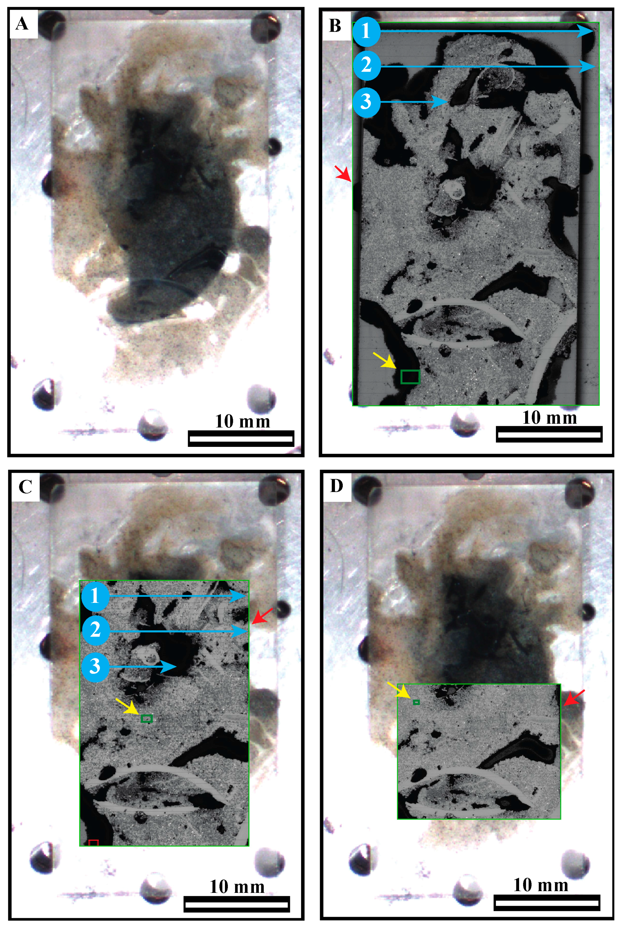
4.1. Beam Stability Issues
4.2. Preparation Considerations
4.3. Potential Problem Areas
4.4. Relevance of Technique
4.5. Mineral Distribution
4.6. Mean Grayscale
4.7. Other Parameters
4.8. Effect of Individual Tile Size
4.9. Future Potential
5. Conclusions
Supplementary Materials
Acknowledgments
Author Contributions
Conflicts of Interest
References
- Tovey, N.K.; Wang, J. An automatic image acquisition and analysis system for a scanning electron microscope. Scanning Microsc. 1997, 11, 211–227. [Google Scholar]
- Buckman, J. Use of automated image acquisition and stitching in scanning electron microscopy: Imaging of large scale areas of materials at high resolution. Microsc. Anal. 2014, 28, 13–15. [Google Scholar]
- Buckman, J.; Mahoney, C.; Bankole, S.; Nazari-Moghaddam, R.; Couples, G.; Lewis, H.; Wagner, T.; Marz, C.; Blanco, V.; Stow, D.; Jamiolahmady, M.; et al. Workflow Model for the Digitization of Shale Rocks. Application of Analytical Techniques to Petroleum System Problems. In Proceedings of the Application of Analytical Techniques to Petroleum Systems Problems, London, UK, 28 February–1 March 2017; pp. 16–17. [Google Scholar]
- Lemmens, H.; Richards, D. Multiscale imaging of shale samples in the scanning electron microscope. In Electron Microscopy of Shale Hydrocarbon Reservoirs; AAPG Memoir 102; Camp, W.K., Diaz, E., Wawak, B., Eds.; AAPG: Tulsa, OK, USA, 2013; pp. 27–36. [Google Scholar]
- Ogura, K.; Yamada, M.; Hirahara, O.; Mita, M.; Erdman, N.; Nielsen, C. Gigantic montages with a fully automated FE-SEM (serial sections of a mouse brain tissue). Microsc. Microanal. 2010, 16, 52–53. [Google Scholar] [CrossRef]
- Deshpande, S.; Kulkarni, A.; Sampath, A.; Herman, H. Application of image analysis for characterization of porosity in thermal spray coatings and correlation with small angle neutron scattering. Surf. Coat. Technol. 2004, 187, 6–16. [Google Scholar] [CrossRef]
- Doktor, T.; Kytyr, D.; Valach, J.; Jirousek, O. Assessment of pore size distribution using image analysis. In Proceedings of the 9thYouth Symposium on Experimental Solid Mechanics, Trieste, Italy, 7–9 July 2010. [Google Scholar]
- Ziel, R.; Haus, A.; Tulke, A. Quantification of the pore size distribution (porosity profiles) in microfiltration membranes by SEM, TEM and computer image analysis. J. Membr. Sci. 2008, 323, 241–246. [Google Scholar] [CrossRef]
- Berrezueta, E.; Gonzálex-Menéndez, L.; Ordóñez-Casado, B.; Olaya, P. Pore network quantification of sandstones under experimental CO2 injection using image analysis. Comput. Geosci. 2015, 77, 97–110. [Google Scholar] [CrossRef]
- Mazurkiewicz, L.; Mlynarczuk, M. Determining rock pore space using image processing methods. Geol. Geophys. Environ. 2013, 39, 45–54. [Google Scholar] [CrossRef]
- Anselmetti, F.S.; Luthi, S.; Eberli, G.P. Qualitative characterization of carbonate pore systems by digital image analysis. AAPG Bull. 1998, 82, 1815–1836. [Google Scholar]
- Haines, T.J.; Neilson, J.E.; Healy, D.; Michie, E.A.H. The impact of carbonate texture on the quantification of total porosity by image analysis. Comput. Geosci. 2015, 85, 112–125. [Google Scholar] [CrossRef]
- Anovitz, L.M.; Cole, D.R. Characterization and analysis of porosity and pore structures. Rev. Mineral. Geochem. 2015, 80, 61–164. [Google Scholar] [CrossRef]
- Van der Land, C.; Wood, R.A.; Wu, K.; Van Dijke, M.I.J.; Jiang, Z.; Corbett, P.W.M.; Couples, G.D. Modelling the permeability evolution of carbonate rocks. Mar. Pet. Geol. 2013, 48, 1–7. [Google Scholar] [CrossRef]
- Robinet, J.C.; Sardini, P.; Siitari-Kauppi, M.; Prêt, D.; Yven, B. Upscaling the porosity of the Callovo-Oxfordian mudstone from the pore scale to the formation scale; insights from the 3H-PMMA autoradiography technique and SEM BSE imaging. Sediment. Geol. 2015, 321, 1–10. [Google Scholar] [CrossRef]
- Hellmuth, K-H.; Siitari-Kauppi, M. Investigation of the Porosity of Rocks; STUK-B-VALO63; Finnish Centre for Radiation and Nuclear Safety (STUK): Helsinki, Finland, 1990. [Google Scholar]
- Hurley, N. Microporosity quantification using confocal microscopy. In Proceedings of the Mountjoy Carbonate Research Conference, Carbonate Pore Systems, Austin, TX, USA, April 2017. [Google Scholar]
- Buckman, J.O.; Corbett, P.W.M.; Mitchell, L. Charge contrast imaging (CCI): Revealing enhanced diagenetic features of a coquina limestone. J. Sediment. Res. 2016, 86, 734–748. [Google Scholar]
- Catto, B.; Jahnert, R.J.; Warren, L.V.; Varejao, F.G.; Assine, M.L. The microbial nature of laminated limestones: Lessons from the Upper Aptian, Araripe Basin, Brazil. Sediment. Geol. 2016, 341, 304–315. [Google Scholar] [CrossRef]
- Warren, L.V.; Varejão, F.G.; Quaglio, F.; Simões, M.G.; Fürsich, F.T.; Poiré, D.G.; Catto, B.; Assine, M.L. Stromatolites from the Aptian Crato Formation, a hypersaline lake system in the Araripe Basin, northeastern Brazil. Facies 2017, 63, 3. [Google Scholar] [CrossRef]
- Leslie, A.G.; Browne, M.A.E. Scotland’s coal—A life after extraction. Edinb. Geol. 2015, 58, 11–17. [Google Scholar]
- Francus, P.; Pirard, E. Testing for sources of errors in quantitative image analysis. In Image Analysis, Sediments and Paleoenvironments; Developments in Paleoenvironmental Research; Volume 7, Francus, P., Ed.; Springer: Dordrecht, The Netherlands, 2005; pp. 87–102. [Google Scholar]
- Grove, G.; Jerram, D.A. jPOR: An ImageJ macro to quantify total optical porosity from blue-0stained thin sections. Comput. Geosci. 2011, 37, 1850–1859. [Google Scholar] [CrossRef]
- Berrezueta, E.; Ordóñez-Casado, B.; Bonilla, W.; Banda, R.; Castroviejo, R.; Carrión, P.; Puglla, S. Ore petrography using optical image analysis: application to Zaruma-Portovelo deposit (Ecuador). Geosciences 2016, 6. [Google Scholar] [CrossRef]


| Sample | Laminite | Coquina | Spireslack | Antrim | ||
|---|---|---|---|---|---|---|
| Tile Width (µm) | 50 | 518 | 259 | 518 | 1000 | 2000 |
| Tile Pixel Dimensions | 768 × 512 | 768 × 512 | 768 × 512 | 768 × 512 | 768 × 512 | 768 × 512 |
| Grid Size | 206 × 33 | 87 × 67 | 165 × 152 | 39 × 48 | 19 × 47 | 9 × 23 |
| Total Number Tiles | 6798 | 5829 | 25,080 | 1872 | 893 | 207 |
| Time Taken | 10 h | 8 h | 35 h | 3 h | 1.5 h | 20 min |
| Pixel Resolution | 6.51 nm | 674 nm | 337 nm | 674 nm | 1.3 µm | 2.6 µm |
| Sample | Antrim (2 mm) | Antrim (1 mm) | Antrim (518 µm) | Coquina (518 µm) | Spireslack (259 µm) | Laminite (50 µm) |
|---|---|---|---|---|---|---|
| Minimum | 1 | 0 | 0 | 0 | 1 | 3 |
| Maximum | 100 | 100 | 100 | 61 | 80 | 83 |
| Average | 23 | 24 | 25 | 5 | 9 | 18 |
| Modal | 4 | 2 | 3 | 1 | 9 | 10 |
| Sample | Antrim (2 mm) | Antrim (1 mm) | Antrim (518 µm) | Coquina (518 µm) | Spireslack (259 µm) | Laminite (50 µm) |
|---|---|---|---|---|---|---|
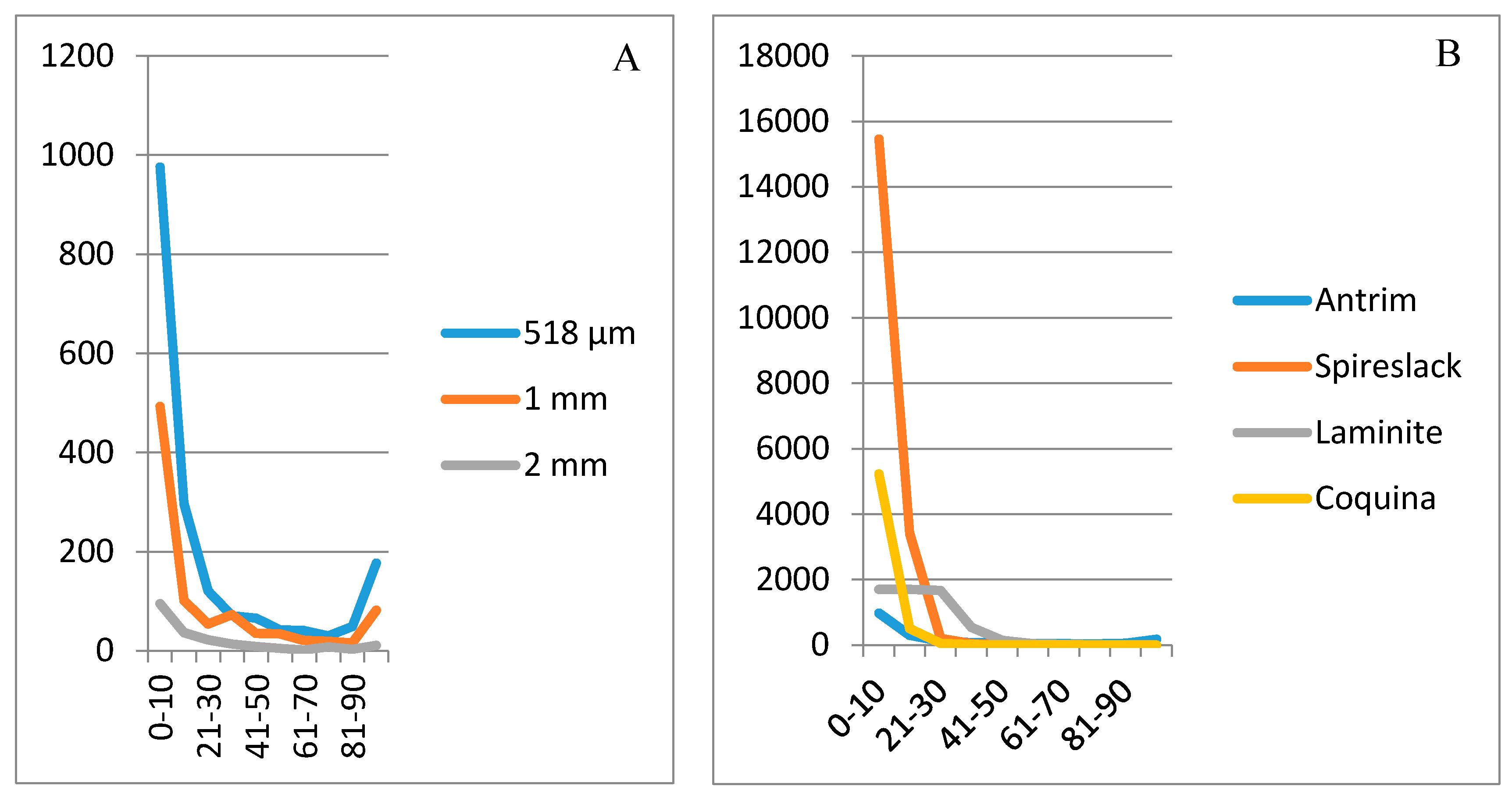
| 0–10% | 95 | 493 | 976 | 5225 | 15,463 | 1697 |
| 11–20% | 37 | 102 | 297 | 503 | 3413 | 1698 |
| 21–30% | 22 | 54 | 121 | 53 | 204 | 1667 |
| 31–40% | 14 | 73 | 71 | 13 | 47 | 538 |
| 41–50% | 9 | 35 | 66 | 4 | 15 | 148 |
| 51–60% | 5 | 34 | 42 | 0 | 22 | 48 |
| 61–70% | 2 | 21 | 41 | 1 | 17 | 16 |
| 71–80% | 8 | 19 | 30 | 0 | 3 | 2 |
| 81–90% | 3 | 16 | 49 | 0 | 0 | 0 |
| 91–100% | 11 | 82 | 177 | 0 | 0 | 0 |
© 2017 by the authors. Licensee MDPI, Basel, Switzerland. This article is an open access article distributed under the terms and conditions of the Creative Commons Attribution (CC BY) license (http://creativecommons.org/licenses/by/4.0/).
Share and Cite
Buckman, J.; Bankole, S.A.; Zihms, S.; Lewis, H.; Couples, G.; Corbett, P.W.M. Quantifying Porosity through Automated Image Collection and Batch Image Processing: Case Study of Three Carbonates and an Aragonite Cemented Sandstone. Geosciences 2017, 7, 70. https://doi.org/10.3390/geosciences7030070
Buckman J, Bankole SA, Zihms S, Lewis H, Couples G, Corbett PWM. Quantifying Porosity through Automated Image Collection and Batch Image Processing: Case Study of Three Carbonates and an Aragonite Cemented Sandstone. Geosciences. 2017; 7(3):70. https://doi.org/10.3390/geosciences7030070
Chicago/Turabian StyleBuckman, Jim, Shereef A. Bankole, Stephanie Zihms, Helen Lewis, Gary Couples, and Patrick W. M. Corbett. 2017. "Quantifying Porosity through Automated Image Collection and Batch Image Processing: Case Study of Three Carbonates and an Aragonite Cemented Sandstone" Geosciences 7, no. 3: 70. https://doi.org/10.3390/geosciences7030070