Structure of Volatile Conduits beneath Gorely Volcano (Kamchatka) Revealed by Local Earthquake Tomography

Abstract

Gorely is an active volcano located 75 km from Petropavlovsk-Kamchatsky, Kamchatka. In 2010–2015, it exhibited strong activity expressed by anomalously high gas emission. In 2013–2014, we deployed a temporary network consisting of 20 temporary seismic stations that operated for one year. We selected 333 events with 1613 P-wave and 2421 S-wave arrival times to build the first tomographic model of this volcano. The seismic model was carefully verified using a series of synthetic tests. Our tomographic model provides a mechanism for volatile feeding of Gorely. An unexpected feature of the model was low Vp/Vs ratios; below 1.4 in some parts. One reason for such low Vp/Vs ratios is gas contamination due to magma degassing. In the central part of the model, directly underneath the Gorely crater, we observe a 2.5 km wide and 1.5 km thick seismic anomaly with a very high Vp/Vs ratio of up to 2. This may represent a magma reservoir with a high melt and/or volatile content. The upper limit of this anomaly, 2.5 km below the surface, may indicate the degassing level, which coincides with the most intense seismicity. Below this reservoir, we observe another columnar high Vp/Vs ratio anomaly. This can be interpreted as a conduit bringing magma and fluids from deeper sources.

1. Introduction

Studying the deep structure beneath active volcanoes is important for understanding how magma and volatile plumbing systems work. This information may reveal the general mechanisms of magma source development, and provide useful criteria for forecasting eruptions. Volcanic research using seismic methods is challenging because active volcanoes are represented by highly heterogeneous, strongly scattered, and rapidly varying geologic media. Examples of fast velocity changes beneath volcanoes can be found in [1,2,3]. Recent studies of different volcanoes around the world [1,3,4,5,6,7] have shown that each appear to be unique, with specific features. Here, we present the first seismic model of Gorely volcano in Kamchatka (Russia), corresponding to 2013–2014 when a temporary seismic network was installed by the Trofimuk Institute of Petroleum Geology and Geophysics.

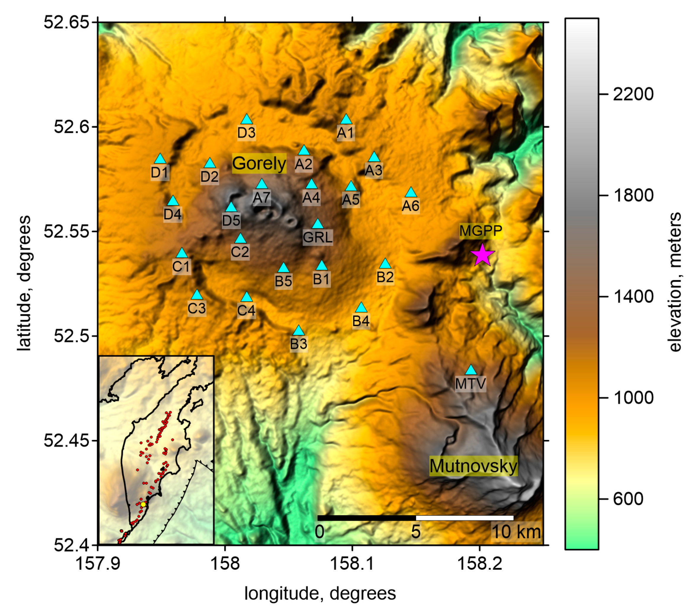
Gorely volcano has a total height of 1800 m, and is located 75 km south-west from Petropavlovsk-Kamchatsky, which is the main city of in Kamchatka, and 25 km from the western coast of Kamchatka. Together with the neighboring Mutnovsky volcano, it forms a common geothermal area with numerous fumaroles and geothermal sources. The Mutnovsky Geothermal Power Plant (MGPP) lies within this area (Figure 1). It has a capacity of 50 MW and is fed by hot underground steam associated with activity from these two volcanoes.

Gorely volcano is located inside a circular caldera approximately 12–15 km in diameter that is clearly observable on topographic maps (Figure 1). This caldera was formed by a large explosive eruption of the Proto-Gorely that ejected more than 100 km³ of material approximately 38,000 years ago [8,9]. After this event, the volcano continued to be active, but it changed composition from andesitic to basaltic [10,11]. Ongoing moderate basaltic to basalt-andesitic eruptions have created an edifice of ~800 m elevation with respect to the caldera bottom. Today, Gorely volcano is a complex structure combining three to five adjoining stratovolcanoes with 11 summit craters and more than 30 flank cones associated with several fissures [8,12]. The recent eruptions of Gorely vary from moderate lava flows to explosive eruptions ejecting a significant amount of ash that, in some cases, reached Petropavlovsk-Kamchatsky [13]. Recorded eruptions occurred in 1828, 1832, 1855, 1869, and 1929–1930 [14], and in May 1931, 1941, and December 1961 [15]. The most recent lava eruption occurred in 1984–1986 [16]. Since 1978–1979, fumarole activity has been continuous in one or several craters. From 2010 to 2015, Gorely volcano was in an active phase expressed by an increase of seismic activity and the presence of tremors. During this time, there was considerable gas emission (mostly consisting of water steam) from a single fumarole in the main crater, which reached 11,000 tons per day [17].

Because of the explosive eruption potential of Gorely and its close proximity to populated areas of Kamchatka, it has been studied for decades using different geologic, geochemical, and geophysical methods. Geophysical investigations, including magnetotelluric surveys and gravity measurements, were performed in the Gorely and Mutnovsky area in the 1980s with the purpose of planning MGPP construction [8]. However, the results of these studies are not openly available. Seismicity beneath Gorely has been investigated since 1984 [18,19] by a permanent seismic station GRL (Figure 1) deployed by the Kamchatkan Branch of Geophysical Survey (KBGS). Two other seismic stations on the Asacha (25 km south-west from Gorely) and Mutnovsky (16 km south-east from Gorely) volcanoes enable approximate location of seismic events; however, the accuracy of the source parameters is low. No other seismic investigations have been performed on Gorely volcano.

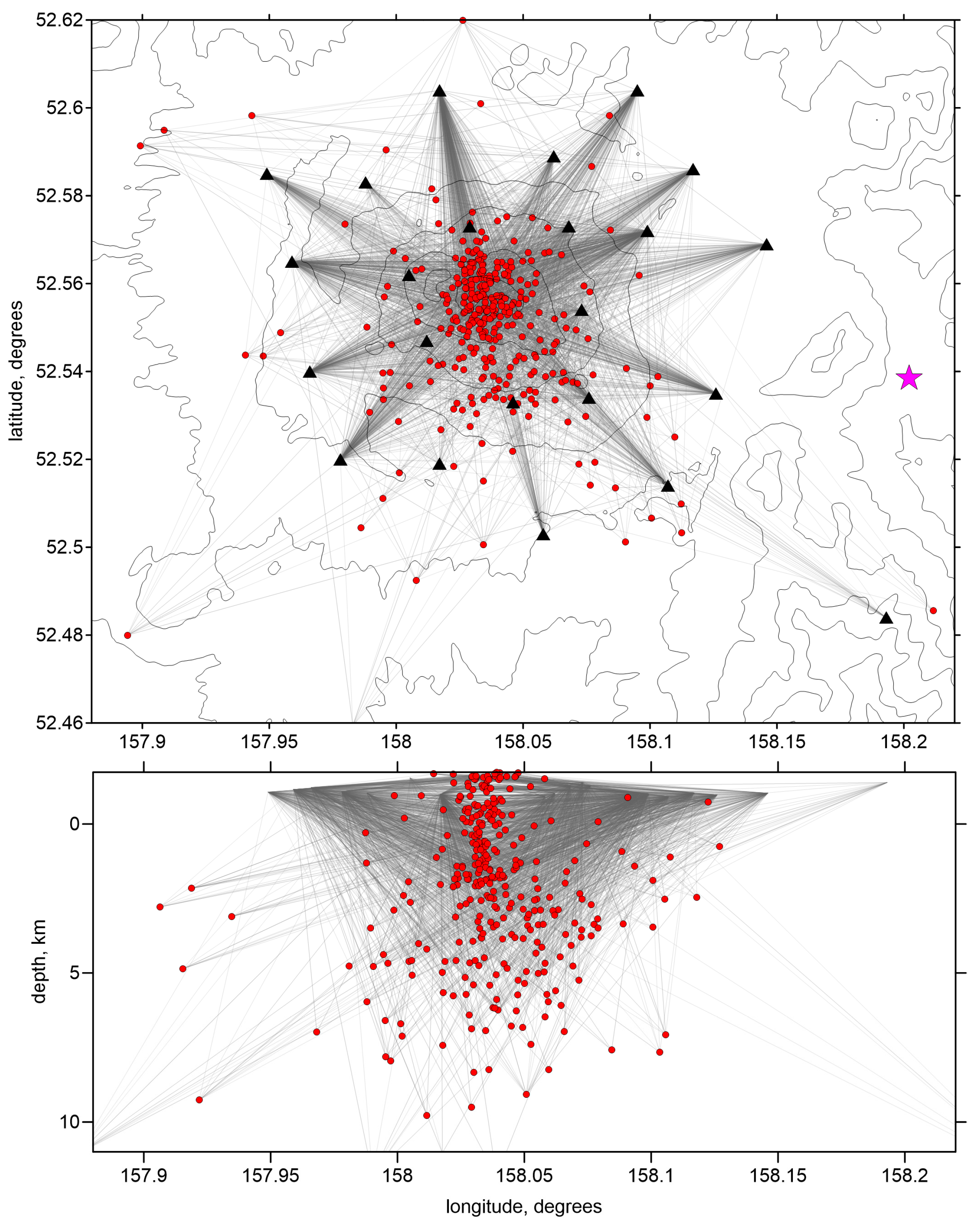
During the recent period of activity, we deployed a network of 21 seismic stations on the volcanic edifice and caldera rim. The purpose of this campaign was to investigate the seismic structure beneath the volcano and to accurately localize seismicity within the edifice. Here, we present the results of this research.

2. Data Description and the Algorithm

To study the seismic structure beneath Gorely volcano, we deployed a network of 20 portable stations on the volcano flanks and surrounding areas (Figure 1). Each station consisted of a three-component broadband sensor CME-4111-LT (R-sensors, Moscow, Russia) (with a period of up to 30 s) and data loggers (Baykal-ACN87 or 88, R-sensors, Novosibirsk, Russia), both of which were manufactured in Russia. The recording time was synchronized using GPS receivers available for each station. At all stations, data were recorded with a frequency of 100 samples per second. Continuous operation of the stations for one year was enabled by sets of ten chemical batteries (Baken-AZ-1, UralElement, Verchniy Ufaley, Russia) with a total capacity of 700 Ah and an output voltage of 12–14 V. The stations were deployed in August 2013 and removed in July 2014. Unfortunately, the full set of stations operated for only three months, after which some equipment became unusable due to various reasons (freezing of batteries, flooding, bear attack, etc.). At the end of the experiment, only six stations were working correctly. For this reason, we processed only the data during the first three months of the network deployment. In addition to data collected at the portable stations, we used the continuous records of three KBGS permanent stations deployed on Gorely and neighboring Mutnovsky and Asacha volcanoes.

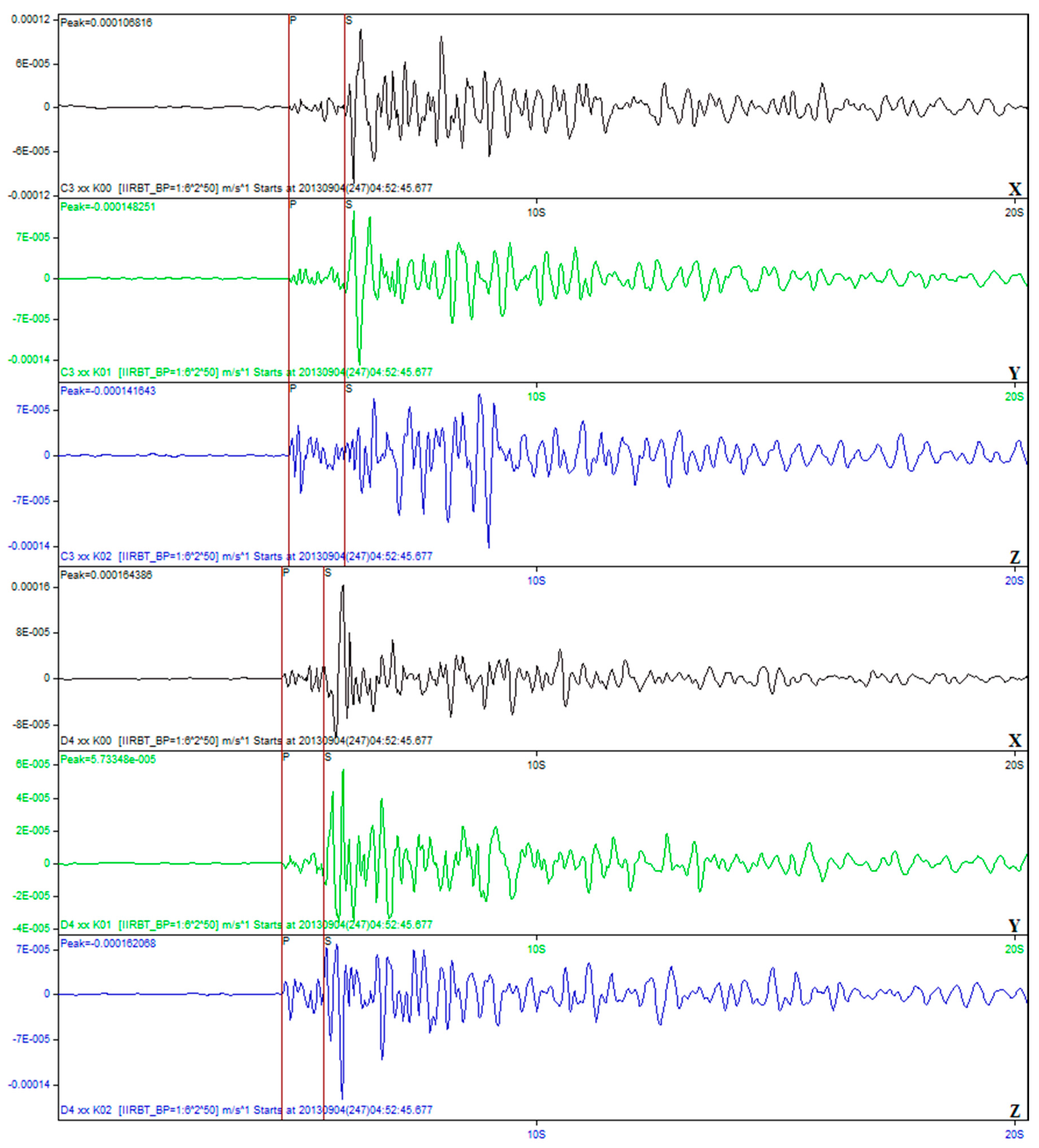
Identification of seismic events and picking of P and S wave arrival times were performed manually using the DIMAS software (version 11 July 2013) designed specifically by KBGS to analyze volcanic seismicity [20]. To identify relevant events, we used a band-pass filter in the range of 2–8 Hz. Most of the seismic activity was associated with tremors and drum-bit events, which could not be used for tomography. On some days, the KBGS reported more than 200 events; however, they were mostly identified as drum-beats events or tremors that are not suitable for time picking. We were only able to find 360 local earthquakes with detectable P and/or S wave arrivals. An example of the processing procedure for one such event using the DIMAS software is presented in Figure 2. The piking errors were strongly dependent on the magnitudes of events and on the recording conditions. For weak events, the error was maximum and reached 0.5 s for both P and S-waves. The locations of all identified events are shown in Figure 3.

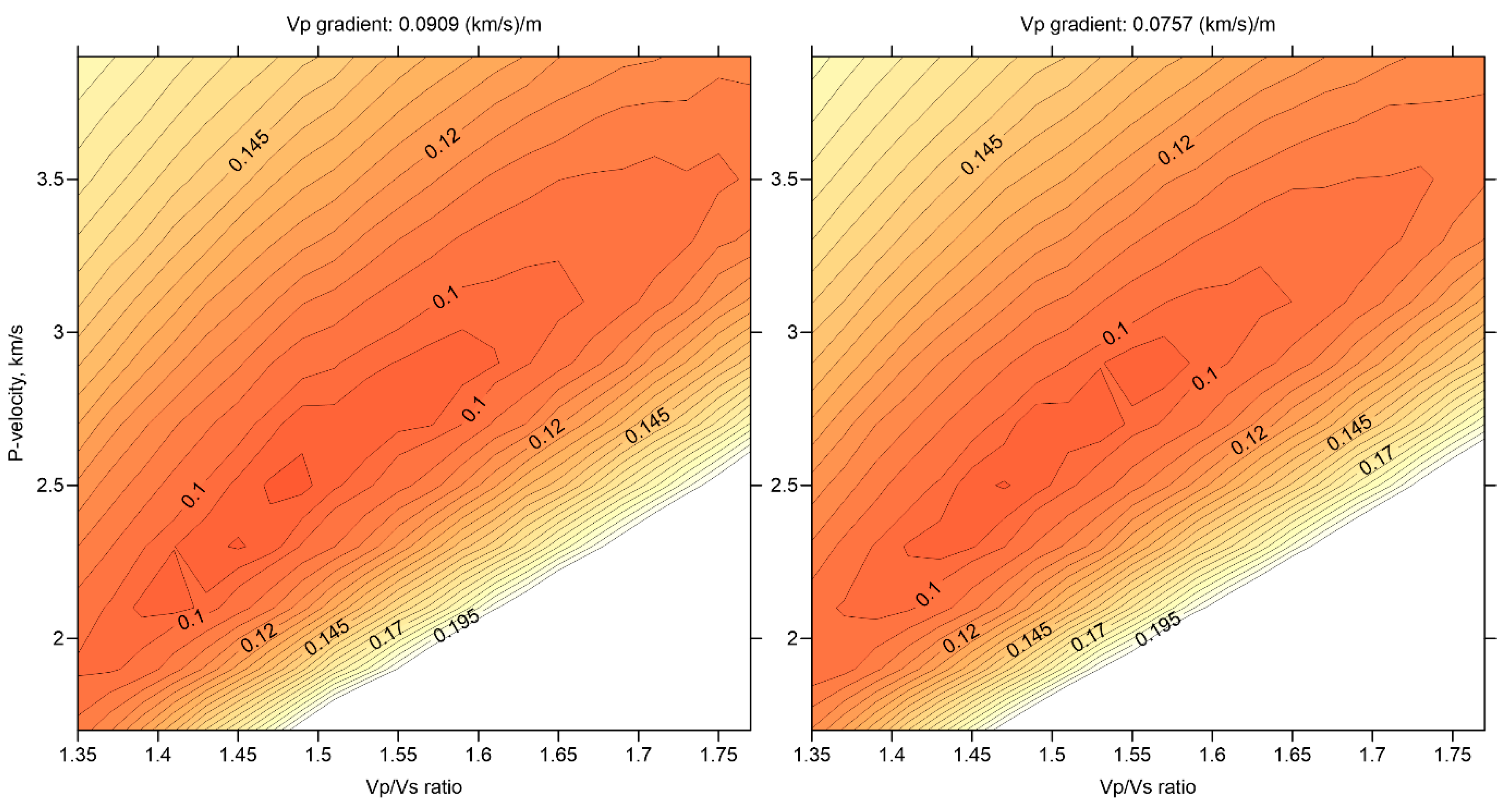
Preliminary source locations were calculated using a grid search method that ensured robust hypocenter determination corresponding to the global extreme of the target function [21]. To speed up the calculations, we computed travel times by integration along straight lines using velocity according to the 1D starting model. For the existing source-receiver configurations, the deviations of the 1D-velocity-based rays from the straight lines are relatively small; thus this method appeared to be an adequate approximation for the case of Gorely. Before starting the tomographic inversion, we searched for the optimum reference 1D velocity model. At this stage, we calculated source locations in a series of 1D models and compared the computed data fit as mean residual deviations in the L1 norm, which is less sensitive to the presence of outliers. Each velocity model had a constant depth gradient and a constant Vp/Vs ratio. We conducted a grid search for the P-wave velocity in the uppermost level at 3 km a.s.l. in the range of 1.7 km/s to 3.9 km/s with an increment of 0.2. For the Vp/Vs ratio, the grid search ranged from 1.35 to 1.77 with an increment of 0.02. Furthermore, we considered several cases with different gradients of P-wave velocity. Figure 4 presents the results of the grid search optimization for two velocity gradients: 0.0909 (km/s)/km and 0.0757 (km/s)/km. In all cases, we obtained unexpectedly low values of Vp/Vs ratio, ranging between 1.45 and 1.55.

Further optimization of the reference model was made after several complete cycles of full tomographic inversion. After obtaining the tomographic inversion results, we calculated the average P and S wave velocities at certain depths (0 and 4 km depth), and used them to define the starting 1D velocity model for the next cycle. After repeating several times, we obtained the model indicated in

Table 1. Reference velocity distribution used in the starting velocity model for tomographic analysis.

Depth (km)	Vp (km/s)	Vs (km/s)
0	2.71	1.75
4	2.83	1.84
30	5.1	3.19

, which provides an approximate balance of positive and negative anomalies in the final tomographic model. Above sea level, the velocities are approximated according to the gradient in the first layer.

To select data for tomographic analysis, we used two criteria: (1) the total number of P and S picks per event should not be less than 6, and (2) the value of the residuals after the preliminary inversion step in the 1D model should not be larger than 0.5 s. As a result, we selected 333 events with 1613 P-wave arrivals and 2421 S-wave arrivals (12.1 picks per event on average). Note that, in this dataset, there is a larger amount of S-wave arrivals because they had larger amplitudes and they had clearer onsets. (Figure 2).

For the tomographic inversion, we used the LOTOS (Local Tomography Software) code for local earthquake travel-time tomography [22]. Based on the arrival times of P and S waves, the code performs iterative calculations and derives the 3D distributions of P and S velocities, and the distribution of local events. One iteration includes subsequent source location, matrix calculation, and inversion. Sources are located in the updated 3D velocity models. In this case, travel times and ray paths are calculated using the bending algorithm of ray tracing. Note that the vertical coordinates of the sources are limited by the topography; thus, the events can be located above sea level.

The velocity distributions were parameterized using a set of nodes distributed only in areas where there were rays. In map view, the nodes were regularly distributed (with the spacing of 0.5 km in our case), whereas in the vertical direction, the distance between nodes was set according to ray density (but it should not be smaller than a predefined value, 0.3 km in our case). To minimize any artefacts related to node geometry, we performed the inversions with four grids with different basic azimuths of node distributions (i.e., 0°, 22°, 45°, and 67°). After computing the models for all grids, they were averaged and combined in one regularly spaced model, which was used in the next iteration for source locations.

The inversion was performed using the LSQR method [23,24]. We performed simultaneous inversion for Vp, Vs, and source parameters (with correction for coordinates dx, dy, dz and origin times, dt). Normally, the LOTOS code includes the station corrections but we did not use this option. The flattening of the velocity anomalies was controlled by adding equations with two nonzero elements with opposite signs, which corresponded to all pairs of neighboring nodes. The optimal values of flattening parameters were determined using synthetic modeling that enabled best recovery of the models. Note also that the number of iterations has a similar effect as damping changes. Therefore, we always used five iterations and only varied the flattening parameters. The amplitude damping was not applied in this case.

3. Synthetic Modeling

Before discussing the experimental data inversion results, we present the results of the synthetic modeling. Besides verifying resolution limitations, such tests are important for finding the optimal values of inversion parameters and for evaluating the role of noise in the data. In the LOTOS code workflow, the synthetic modeling follows the realistic procedure of data processing, and simulates the same problems that exist in experimental data processing. Synthetic travel times were computed for the same source-receiver pairs as used in the final iteration of the experimental data inversion. At this step, we used the bending algorithm that conducted tracing of the rays in the synthetic three-dimensional model. The travel times were perturbed by random noise with a magnitude that has similar variance reduction as for experimental data inversion. When starting the recovery of the model, we “forgot” about the true velocity model and perturbed the locations of sources. Then, we conducted the same inversion procedure, as for the experimental data analysis, that starts from the absolute locations of the sources in the starting 1D velocity model (Table 1).

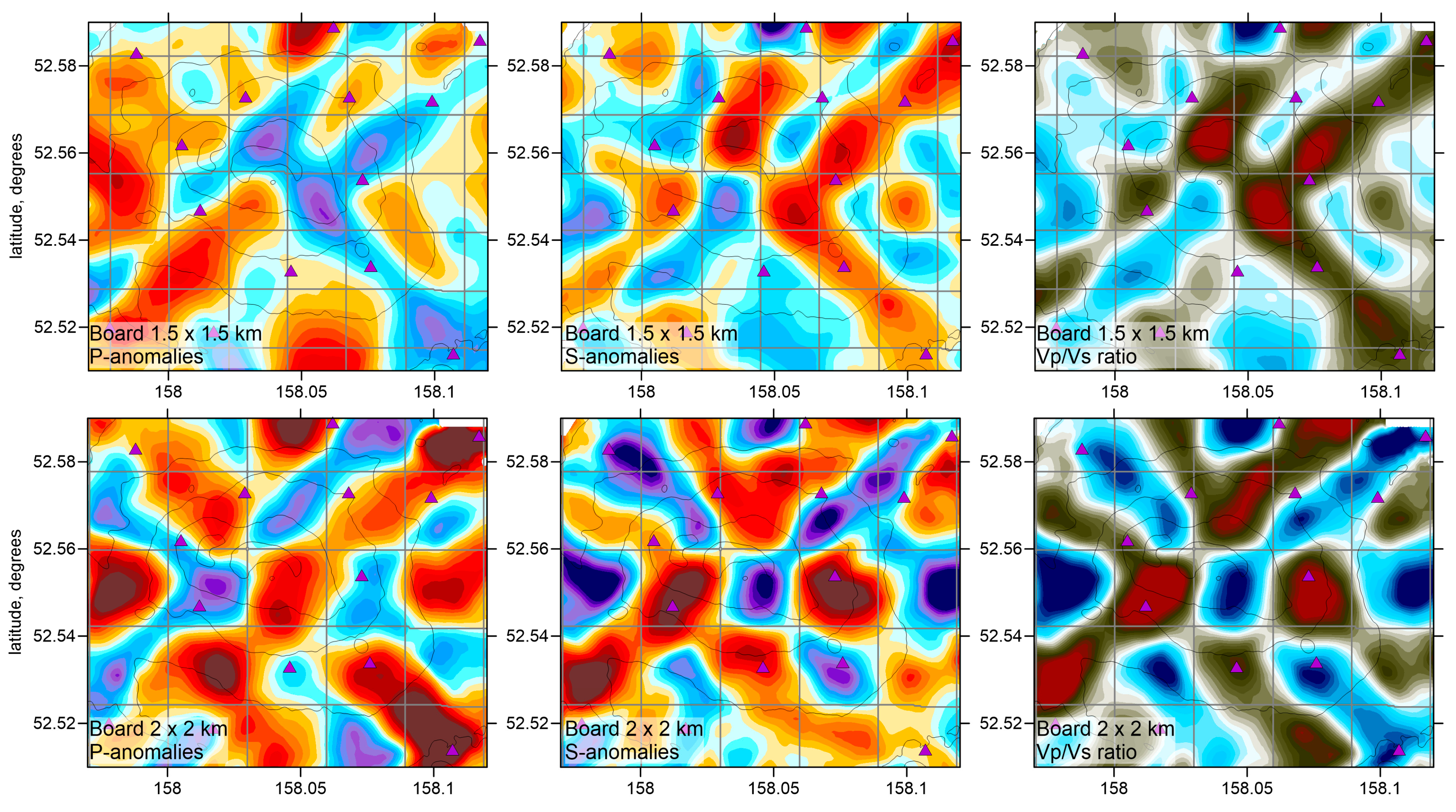
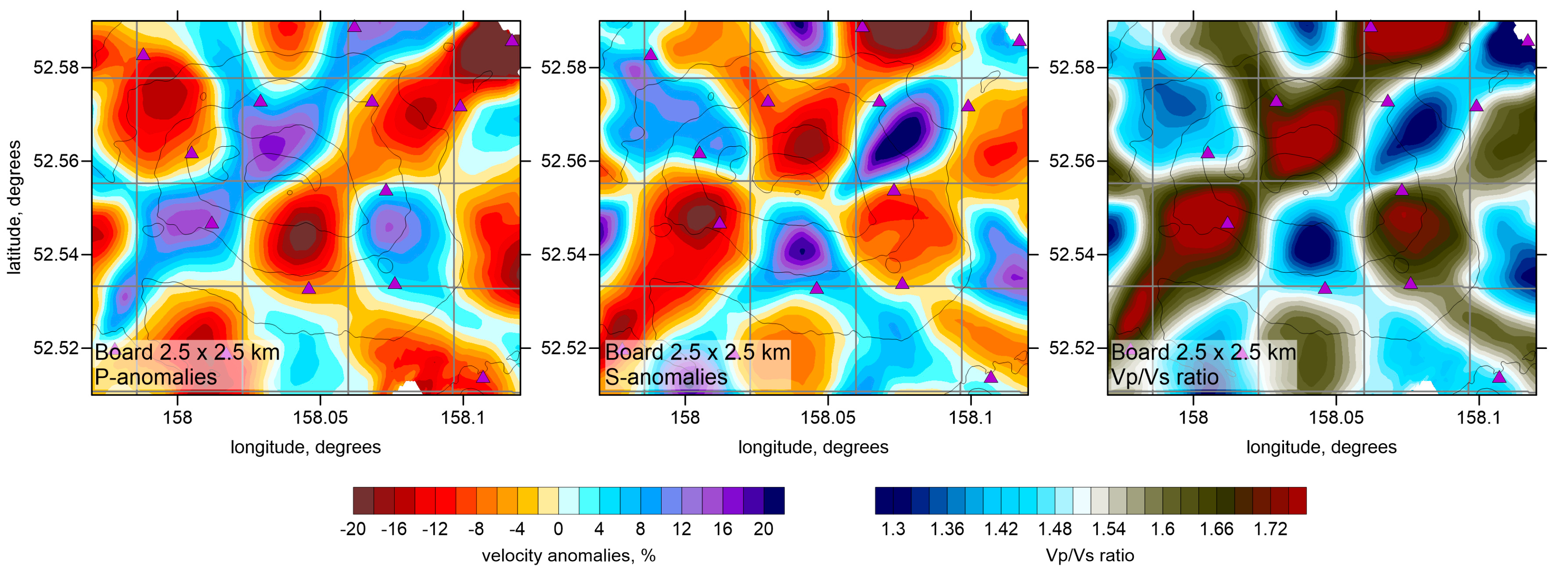
In Figure 5, we present several checkerboard tests aimed to verify the horizontal resolution of the model. In these models, we defined alternating positive and negative anomalies with amplitudes of ±14%. These anomalies remained unchanged with depth. In these tests, we added random noise with a mean magnitude of 0.1 s for both P and S wave data that roughly represent the mean uncertainty of time picking. This error enabled similar variance reductions after inversions of the synthetic models, as in the case of the experimental data inversion. Here, we consider three different models with anomalies having the lateral sizes of 1.5 km, 2 km, and 2.5 km. In all cases, we show the results at 2 km depth b.s.l. The number of iterations and inversion parameters was the same as for the main model derived from the experimental data. In the recovered models, we observe that, for smaller anomalies, the resolution is limited in some parts; however, the larger anomalies are robustly resolved throughout the study area. It is important to note that the Vp/Vs ratio, which was calculated by a simple division of the derived P and S wave velocities, is robustly resolved despite of different sensitivity of the P and S models.

The vertical resolution in passive source tomography is typically lower due to uncertainty in determining the origin time, and the trade-off between source depth and velocity. In Figure 6, we estimate the vertical resolution in two profiles, which will be used to present the main results. The models for each section were calculated independently as separate tests. Each model was defined along each of the vertical sections as periodic rectangular blocks with an unchanging shape across the section. The anomalies are 1 × 1 km² and have amplitudes of ±14%. In both recovery results, we observe significant diagonal smearing of anomalies, which is a typical artifact for this type of modeling. However, beneath the summit, we obtained sufficient resolution to restore three levels of anomalies with opposite signs. This is important for validating the results of the experimental data inversion, in which we observe similar structures. In summary, the major anomalies in the main model, which will be discussed in the following sections, appear to be robust and reliably resolved.

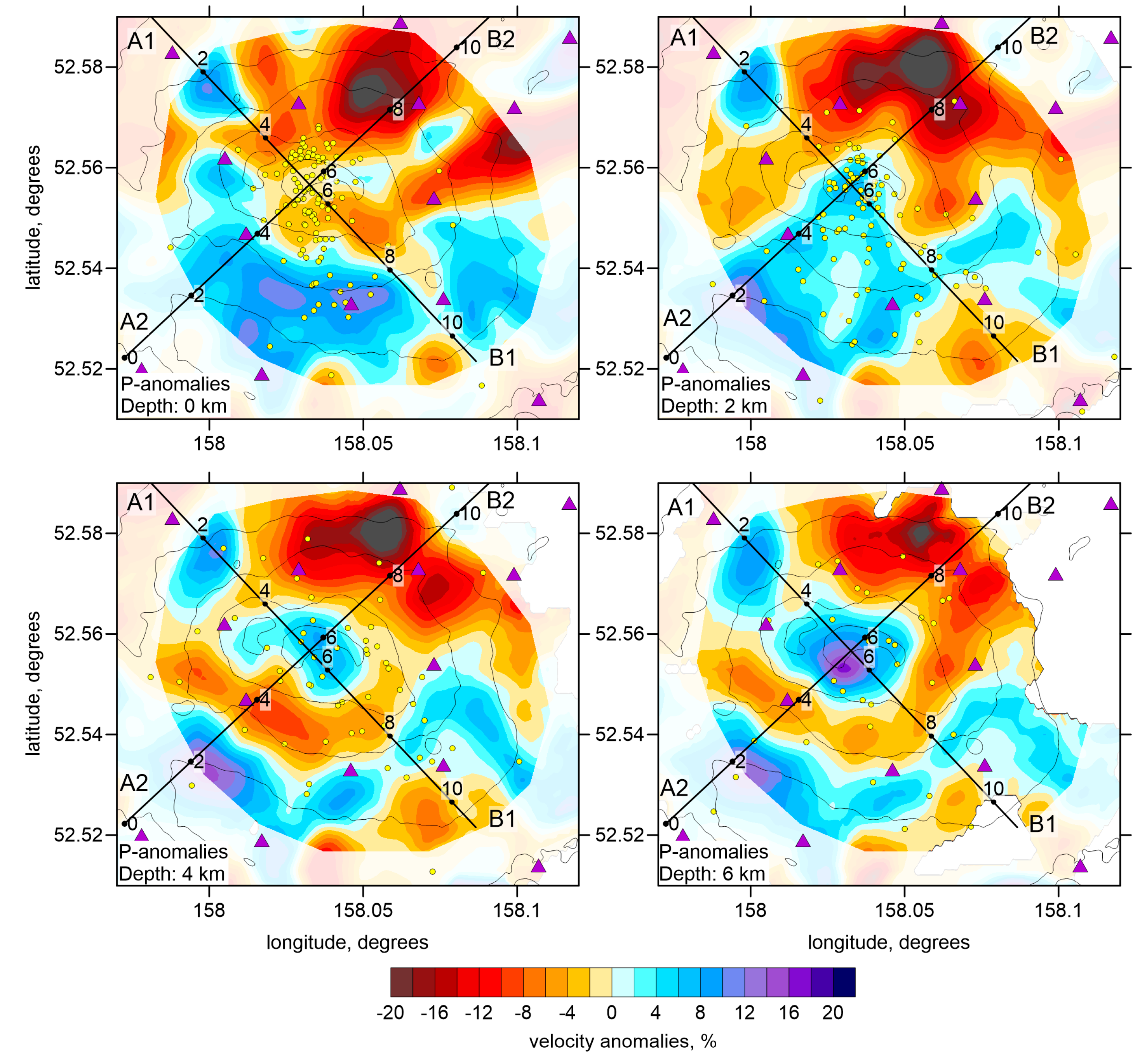
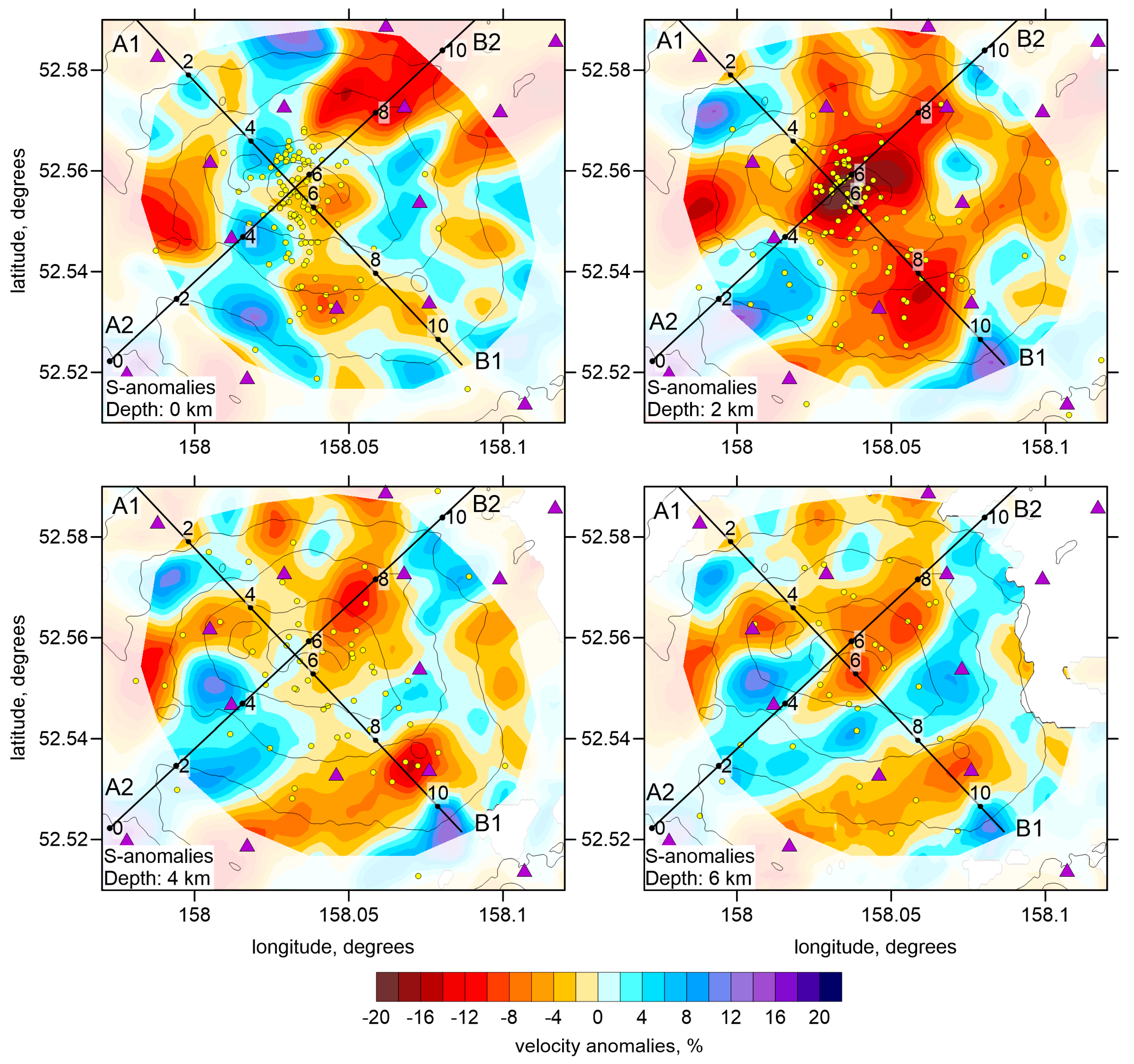
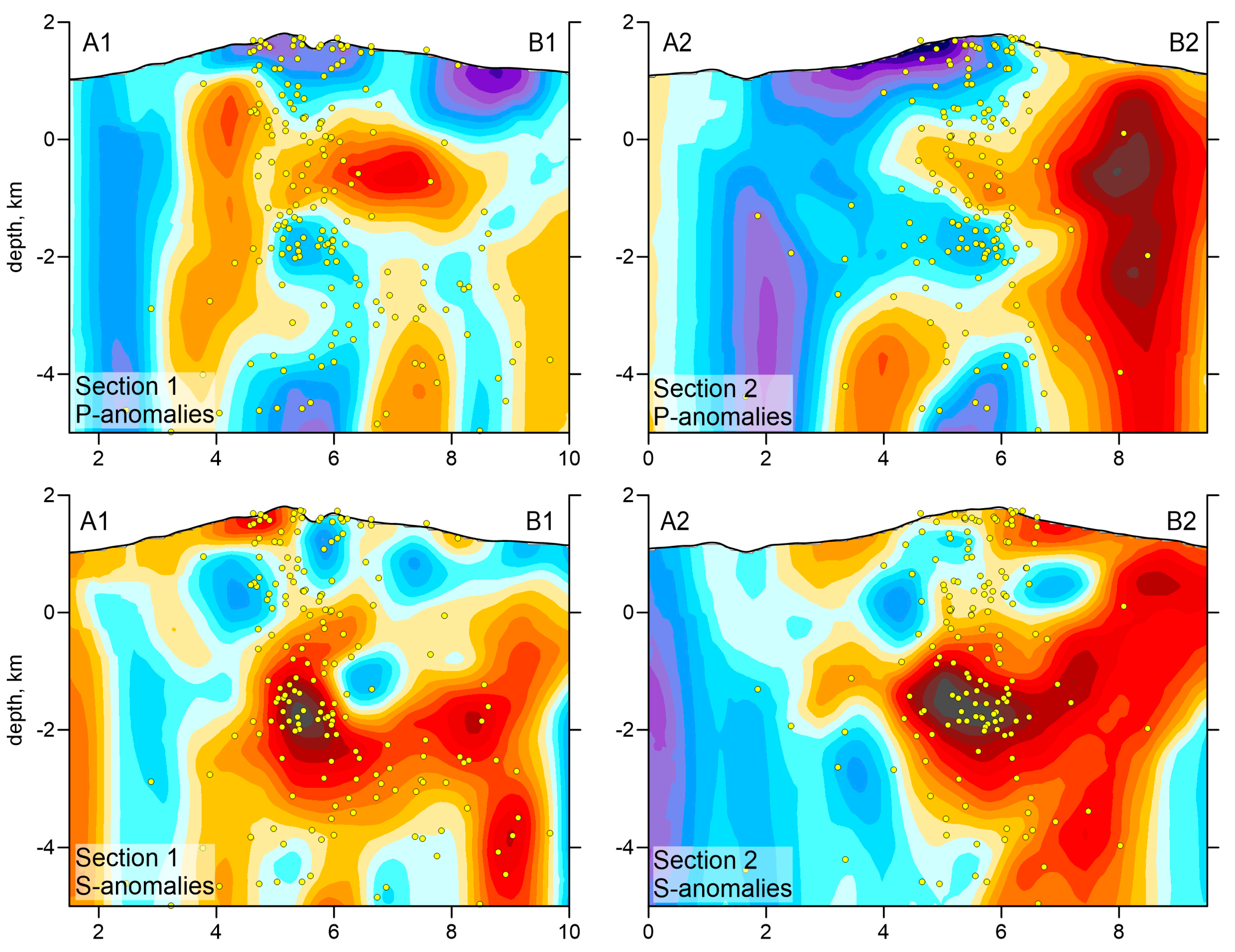
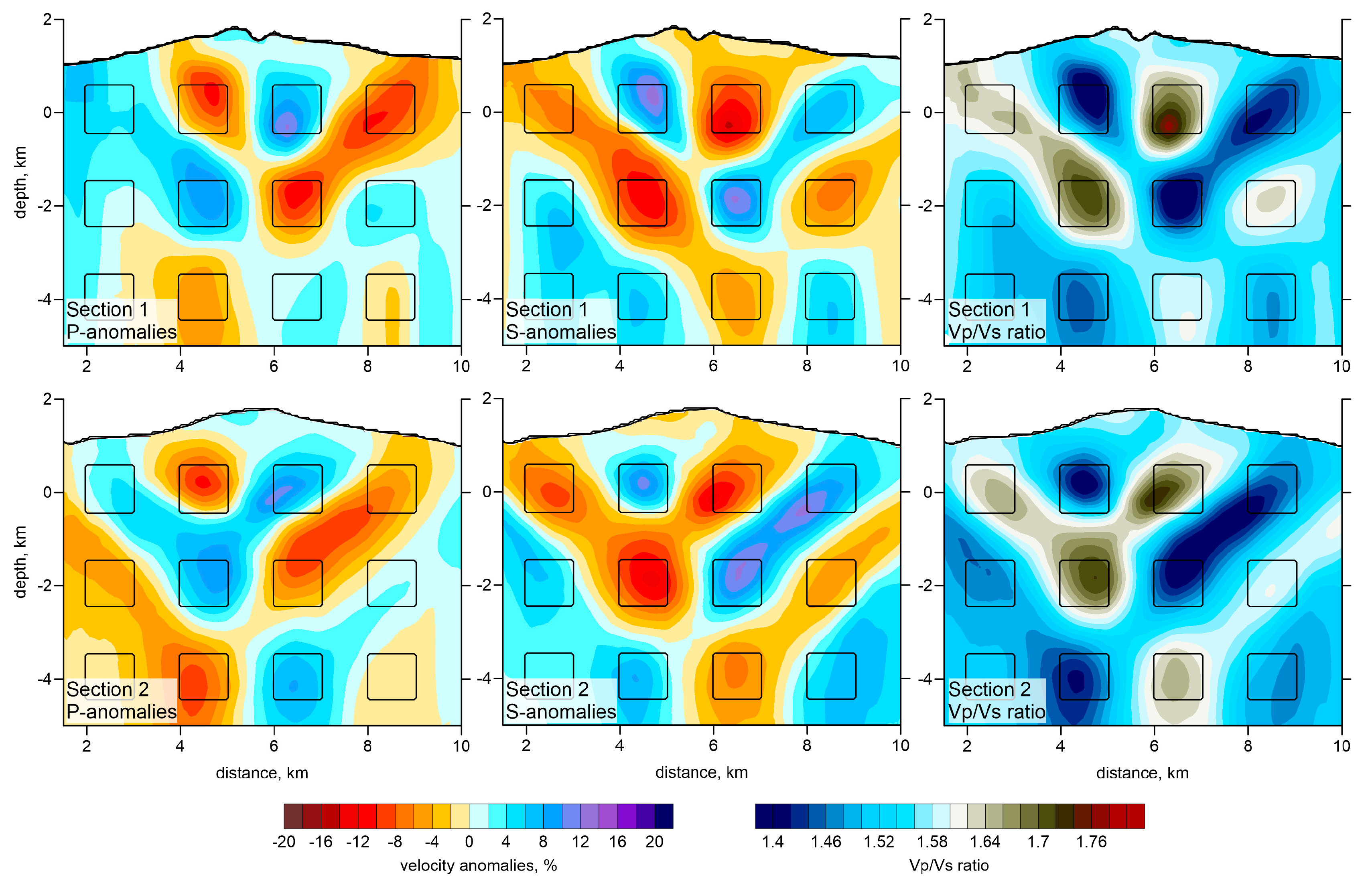
4. Results of Experimental Data Inversion

As a result of tomographic inversion, we obtained the three-dimensional distributions of P and S wave velocities and event locations. The Vp/Vs ratio was obtained by a simple division of the resulting velocities of P-waves to that of S-waves. The stability of this method was proven by a series of synthetic tests presented in Section 3. The resulting P and S wave velocity anomalies, with respect to the reference 1D velocity, and the Vp/Vs ratios are presented in several horizontal and vertical sections in Figure 7, Figure 8, Figure 9 and Figure 10. The seismic models are accompanied with distributions of localized seismic events in the vicinity of the sections.

The derived model appears to be highly heterogeneous. The amplitudes of the P and S anomalies reach 15–20%. In some parts, the P and S anomalies are anti-correlated, which results in intense Vp/Vs ratio variations, ranging from 1.3 to 2. The variance reduction of the residual during five iterations of the inversion is presented in

Table 2. Average absolute values of P- and S-wave residuals (in the L1 norm), and their cumulative reduction during the inversion of experimental data.

Iteration	P-Residual Deviation (s)	P-Residual Reduction (%)	S-Residual Deviation (s)	S-Residual Reduction (%)
1	0.128	0	0.162	0
2	0.118	8.2	0.140	13.6
3	0.113	11.4	0.133	17.5
4	0.113	11.9	0.131	19.0
5	0.110	13.9	0.129	20.1

. For the P and S data, the reduction is 14% and 20%, respectively, which is relatively low. However, similar reductions were observed in some other volcanic studies [2,4]. This can be explained by the relatively small study area. Although anomaly amplitudes are high in the target area, the short ray distances do not allow accumulation of large residuals. They remain at the same order of magnitude as the accuracy of time picking, and the relatively low signal-to-noise ratio does not allow for high variance reduction. However, as was shown in Section 3 by synthetic tests with noisy data, such a low variance reduction does not preclude stable results. The higher reduction for the S-residuals can be explained by the higher sensitivity of S-waves to velocity anomalies (the same values of velocity anomaly lead to a larger residual for S rays than P-rays). Furthermore, in our data, the P-wave arrivals often cannot be picked due to the low amplitude of the signal, which is hard to detect in our noisy seismograms.

5. Discussion

In the horizontal sections of the P-wave velocity anomalies (Figure 7), we observe an isometric high-velocity anomaly just beneath the summit of Gorely. It is surrounded by a circular band of low-velocity. This is a typical volcano-associated structure, which was previously observed in many other studies [1,4,7]. The higher velocity likely corresponds to the volcano edifice consisting of rigid solidified igneous rocks. The surrounding lower velocity anomaly may represent the deposit of soft pyroclasts. The S-velocity structure (Figure 9) shows completely different structures: most intensive low-velocity anomaly is observed beneath the volcano center, in the location where the positive P-velocity anomaly was observed. Such anticorrelation of the P and S-wave velocity anomalies is a typical feature observed in many active volcanoes during their unrests. For example Kasatkina et al. [1] found that beneath the Mt. Redoubt, after beginning of an eruption in 2009, the positive S-wave velocity anomaly changed to a strong negative one, whereas the high P-wave velocity anomaly remained almost unchanged. For the Redoubt eruption, this was explained by strong saturation of the magma sources by fluids and melts that strongly affects the S-velocity. We propose that similar saturation took place beneath the Gorely volcano during its activity period in 2014, when the network was installed.

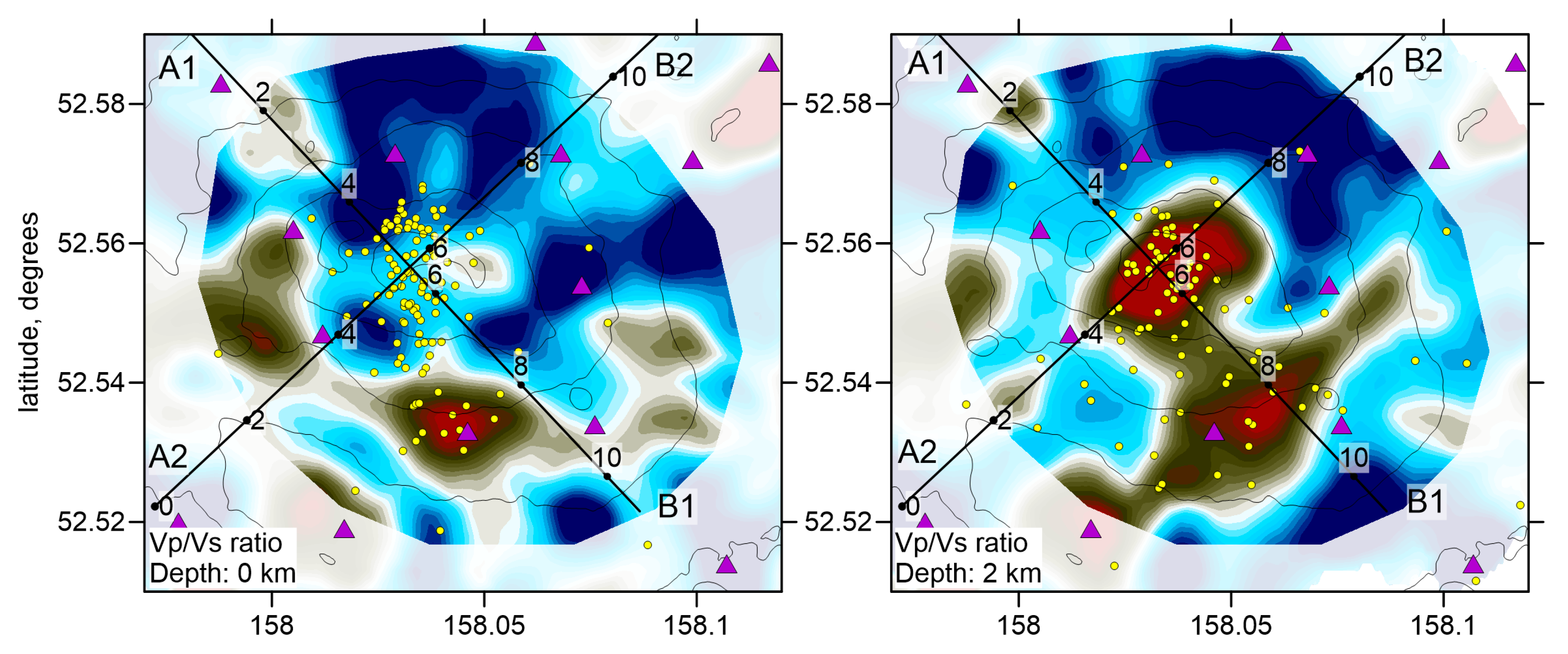
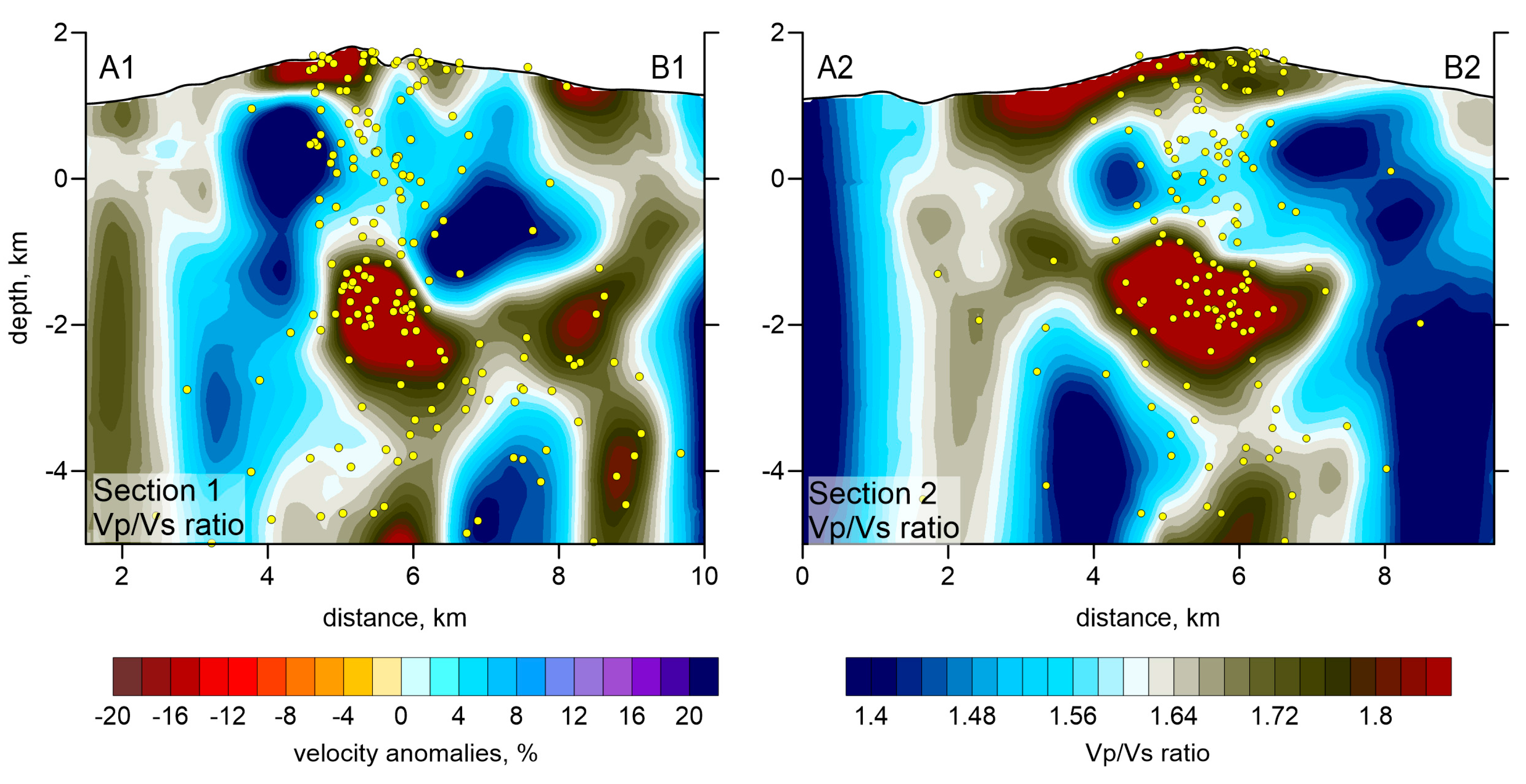
When studying volcano-related structures, the Vp/Vs ratio distribution is often considered one of the most informative parameters, as it appears to be the most sensitive to liquid and gas contents. From the beginning of our processing, we detected a very low average Vp/Vs ratio of 1.5. This was unexpected because volcanic structures are typically associated with the presence of liquids (melts and fluids); thus, a high Vp/Vs ratio was predicted. However, in some volcanic areas, volcanic conduits are associated with low Vp/Vs ratio zones, indicating the presence of gas. For example, in Campi Flegrei, a large low Vp/Vs ratio anomaly [25,26] corresponds to the area of maximum degassing observed on the surface. Similar features have been detected beneath the Yellowstone Caldera [27,28]. Nakajima and Hasegawa [29] detected a columnar anomaly with a low Vp/Vs ratio beneath the Naruko volcano in Japan, and interpreted it as a conduit of degassed volatiles. Similar zones of low Vp/Vs ratio have been observed in the upper layers beneath Mt. Spurr in Alaska [6] and Nevado del Ruiz in Colombia [3]. Both these volcanoes emitted a large amount of gas during observation periods; thus, the anomalously low Vp/Vs ratio was interpreted as saturation of the shallow rocks with gases.

This relationship between gas content and low Vp/Vs ratio is supported by numerous results of laboratory and field experiments [30]. A porous medium saturated with dry gas behaves as a sponge, and thus has a low compression modulus that leads to very low velocity P-waves. The drop in S-wave velocity in such a medium is not as substantial, as the dry matrix may retain the shear strength of the rock. As a result, the Vp/Vs ratio in such a medium is low.

Although the mean Vp/Vs ratio in our study is low, the major finding of our results is a highly heterogeneous anomaly of very high Vp/Vs ratio (up to 2) located just below the main crater at a depth interval of 0.8–2.6 km b.s.l. Within this feature, we observe a high P- and low S-wave velocity anomaly. Such a relationship is observed beneath many active volcanoes, such as Mt. Spurr [6], Redoubt [1], Nevado del Ruiz [3], Klyuchevskoy and Bezymianny volcanoes in Kamchatka [31], and Lunayyir in Saudi Arabia [32]. As compressional waves are more sensitive to composition, a higher P-wave velocity may indicate the presence of magma with a more primitive composition that arrived from deeper reservoirs. Conversely, shear waves are more sensitive to the aggregate state; thus, the low S-wave velocity may indicate the presence of melts and/or contamination with liquid fluids. Therefore, the coexistence of high Vp, low Vs, and a very high Vp/Vs ratio is often considered indicative of an active magma reservoir [31]. In the case of Gorely, the area with the relatively high P-wave velocity and very low S-wave velocity at the depth of around 3 km below surface has a very high Vp/Vs ratio. It may represent a reservoir, which appears to be the source of recent magmatic eruptions [16] and very intensive gas emission [17].

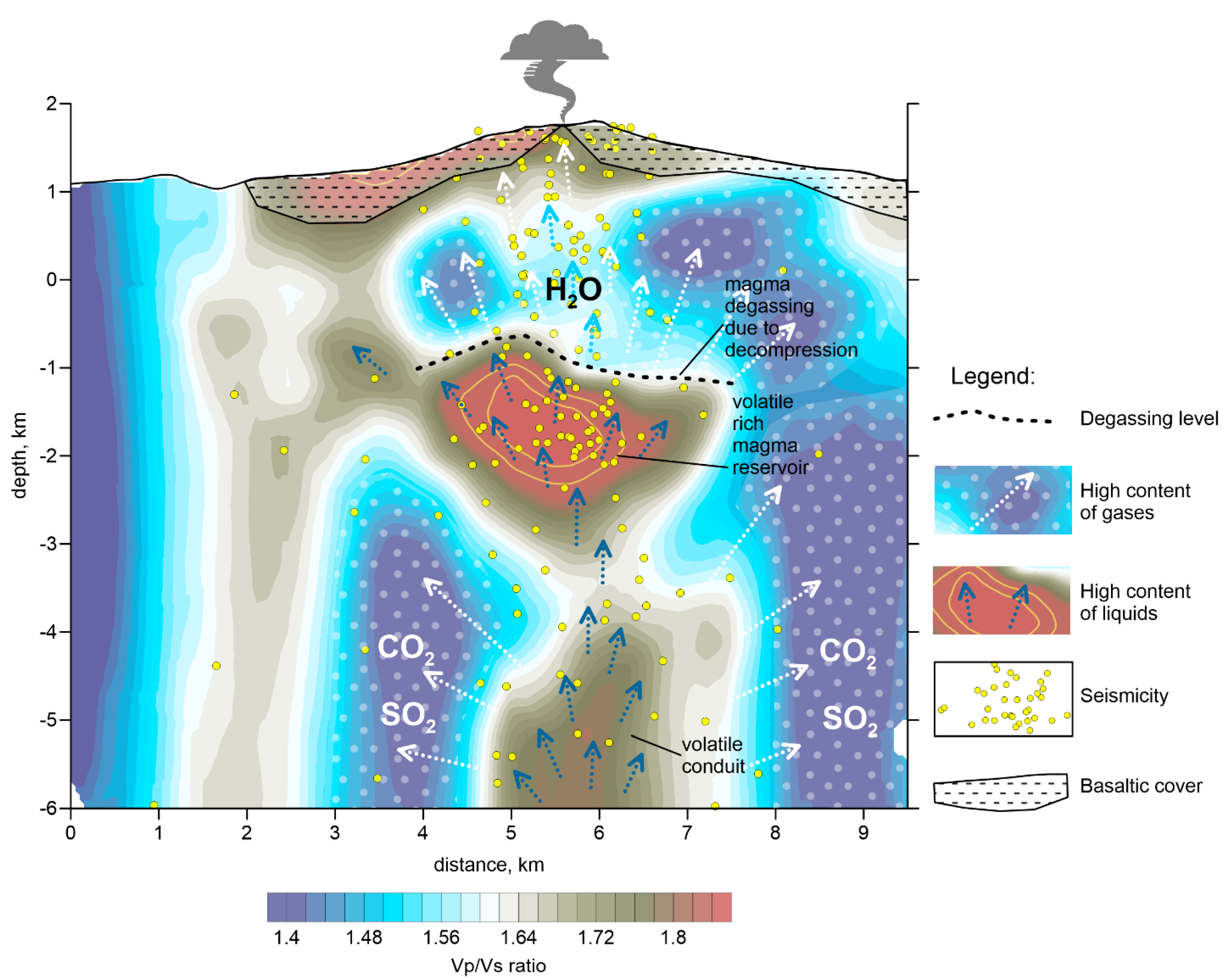
The upper limit of this high Vp/Vs anomaly is located 2.6 km below the surface, and roughly parallel to the topography line. The transition from a high to low Vp/Vs ratio can be interpreted as the degassing level, as schematically shown in Figure 11. A very similar feature was observed beneath the Nevado del Ruiz volcano in Colombia [3] where the transition from high to low Vp/Vs was observed ~2 km below the surface, and was coherent with the relief. We propose that, at Gorely, this boundary represents the degassing level of water saturated in a magma reservoir located at depths of 2–4 km below the surface (reddish anomaly in Figure 11). Note that most seismicity is observed within and above this reservoir, which may represent gradual stages of H₂O extraction from the melt and degassing.

The reservoir-related anomaly appears to extend downward into another high-Vp/Vs anomaly observed below 3 km below surface (Figure 11). This may represent a conduit zone bringing volatiles (mostly H₂O) from deeper sources. This anomaly is surrounded by areas of extremely low Vp/Vs ratio of approximately 1.4, which may be associated with gas-saturated areas. We propose that, at such depths, this might represent traces of CO₂ and SO₂ degassing that occurs at much deeper levels than that of H₂O [33].

The existence of large areas of low Vp/Vs ratio is an unusual phenomenon, which may indicate that Gorely volcano behaves as a large steam boiler with only one safety valve, located in the main crater. During the active period in 2010–2015, the gas flux from this valve reached 11.000 tons per day [17]. The basaltic lava flows forming the edifice of Gorely serve as a rigid cover that prevent gas escape from other locations than the crater. It is notable that the Mutnovsky Geothermal Power Plant lies on the margins of this steam boiler, and uses energy from the volcanic gases that accumulate beneath the volcano.

6. Conclusions

The first temporary network on Gorely volcano, consisting of 20 seismic stations deployed in 2013–2014, provided continuous three-component records during a period of increased gas emission and seismicity. Careful and time-consuming separation of relevant seismic events from drum-bits and tremor activity was required to select sufficient data for a travel-time tomographic analysis. Good resolution of the derived seismic model was proven by a series of synthetic tests.

Optimization of the initial velocity model, as well as further 3D tomography models, revealed unusually low Vp/Vs ratios. In many parts of the model, it is below 1.4. This may indicate substantial contamination of the rocks beneath Gorely by gases. This is supported by gas flux measurements from the central fumarole that reach 11,000 tons per day [17]. In this sense, Gorely volcano is a kind of steam boiler with only one “safety valve” in the main crater to release the accumulated pressure.

At a depth of ~2.5 km, we observe a large anomaly, 2.5 km wide and 1.5 km thick, of very high Vp/Vs ratios, up to 2, in which high Vp coexists with low Vs. A similar relationship exists beneath many other active volcanoes, and such anomalies are often interpreted as active magma reservoirs with high melt and/or liquid fluid contents. In the case of Gorely, this anomaly may represent the main source of recent eruptions and gas emission. The upper limit of this anomaly, located ~2.5 km below the surface, may represent the degassing level where water steam escapes from the magma reservoir. This decompression area corresponds to the area of most intense seismicity. At deeper levels, we observe another columnar high Vp/Vs anomaly zone surrounded by very low Vp/Vs ratios. We propose that this may represent the conduit bringing up volatile-enriched magma. The areas of low Vp/Vs ratio may be associated with contamination by CO₂ and SO₂, which may be released from deeper magma reservoirs.

Based on this new tomography model, we conclude that Gorely volcano is an active thermodynamic machine, where complex aggregate transitions and chemical reactions cause a large amount of gas release. We postulate that this might be the mechanism behind strong explosive eruptions.