Influence of Flow Velocity on Tsunami Loss Estimation


Department of Civil Engineering, Queen’s School of Engineering, University of Bristol, Queen’s Building, University Walk, Bristol BS8 1TR, UK
*
Author to whom correspondence should be addressed.
Geosciences 2017, 7(4), 114; https://doi.org/10.3390/geosciences7040114
Submission received: 30 September 2017
/
Revised: 28 October 2017
/
Accepted: 1 November 2017
/
Published: 7 November 2017
(This article belongs to the Special Issue Interdisciplinary Geosciences Perspectives of Tsunami)
Abstract
:Inundation depth is commonly used as an intensity measure in tsunami fragility analysis. However, inundation depth cannot be taken as the sole representation of tsunami impact on structures, especially when structural damage is caused by hydrodynamic and debris impact forces that are mainly determined by flow velocity. To reflect the influence of flow velocity in addition to inundation depth in tsunami risk assessment, a tsunami loss estimation method that adopts both inundation depth and flow velocity (i.e., bivariate intensity measures) in evaluating tsunami damage is developed. To consider a wide range of possible tsunami inundation scenarios, Monte Carlo-based tsunami simulations are performed using stochastic earthquake slip distributions derived from a spectral synthesis method and probabilistic scaling relationships of earthquake source parameters. By focusing on Sendai (plain coast) and Onagawa (ria coast) in the Miyagi Prefecture of Japan in a case study, the stochastic tsunami loss is evaluated by total economic loss and its spatial distribution at different scales. The results indicate that tsunami loss prediction is highly sensitive to modelling resolution and inclusion of flow velocity for buildings located less than 1 km from the sea for Sendai and Onagawa of Miyagi Prefecture.
1. Introduction
The most recent devastating tsunami that struck the Tohoku region of Japan in 2011 caused a tremendous economic loss. The underestimated tsunami hazard for the coastal areas in Tohoku region prior to the event highlighted deep uncertainty and potential bias in some of the key assumptions in the assessment (e.g., the maximum largest earthquake in the offshore region of Tohoku). A strategy to address this issue is to consider possible scenarios comprehensively in the tsunami hazard assessment. The uncertainty in hazard propagates in the risk assessment, being transformed into tsunami impact parameters (i.e., economic loss). Catastrophe risk assessment is essential for achieving effective risk management to deal with the low-probability high-consequence catastrophes in the global insurance–reinsurance system by transferring financial risks among stakeholders [1,2,3]. Tsunamis are one of the low-probability high-consequence natural disasters, and thus the improved accuracy of tsunami loss estimation can help insurance/re-insurance underwriters to better understand their exposure to catastrophe risks and is beneficial for profitable design of risk transfer instruments [4,5,6].
Tsunami fragility curves convert tsunami hazard intensity into tsunami damage probabilities, and are key components in a tsunami loss estimation framework. Due to different geographical features and tsunami propagation path, tsunami hazard varies within inundated areas significantly. Multiple intensity measures (IM) that describe the extent of tsunami inundation have been proposed, including inundation depth, flow velocity, and momentum flux [3,7,8]. Although inundation depth is the most observable intensity measure in post-tsunami situations and the most common IM in the tsunami risk assessment [9,10,11,12], it cannot be taken as the sole representation of tsunami impact on structures, especially for damage caused by hydrodynamic and debris impact forces that are mainly determined by flow velocity [13,14]. During tsunami events, flow velocity is measurable from particle image velocimetry analysis of videos of survivors [15,16], coastal oceanographic radar tsunami system [17], and satellite altimetry [18]. Therefore, when validated and supplemented by accurate numerical tsunami simulations, reliable estimates of flow velocity can be obtained; they can be used for developing velocity-based tsunami fragility functions. The influence of flow velocity on tsunami fragility has been demonstrated by several studies [7,8,19], but the importance of velocity for tsunami loss has not been explored yet. Existing velocity-based fragility functions [20,21] offer an option to use either inundation depth or flow velocity, which enables the comparison of two intensity measures in risk assessment. However, such comparisons cannot be directly used to evaluate the difference made by flow velocity in addition to inundation depth, since these models are developed for tsunami hazard parameters individually. There is a knowledge gap between importance of velocity for tsunami fragility model development and its influence on tsunami loss estimation; the latter may be more relevant for risk managers who are concerned with financial impact of tsunami disasters.
Moreover, in the context of efficient tsunami IM, momentum flux () is often considered to be a superior hazard indicator for tsunami damage estimation because it captures two fundamental characteristics of tsunami waves, i.e., inundation h and flow velocity v at the same time [7,8,22,23]. However, its observation is almost impossible in post-tsunami damage surveys, and, hence, the tsunami fragility modelling based on momentum flux needs to solely rely on numerical simulations without calibration against actual data—this is a major drawback. In addition, the difference made by momentum flux compared to inundation depth in probabilistic tsunami loss estimation cannot appropriately represent the difference made by v because momentum flux is proportional to h, whereas it is proportional to .
Existing tsunami risk assessments are often carried out using a scenario-based approach focusing on either historical tsunami catalogue or specific critical scenarios, although selected scenarios cannot comprehensively consider all possible situations [24,25,26,27]. This is a critical issue for major tsunami disasters. For instance, spatial slip distributions of a 9.0 earthquake can vary significantly in terms of location and dimension of the earthquake rupture and details of earthquake slips along the rupture plane. It has been demonstrated that the uncertainty in earthquake source characterisation results in significant variability of tsunami loss in coastal regions [28,29,30,31]. In probabilistic tsunami risk analysis, several studies adopted a stochastic approach where the seismic source is characterised by magnitude and average slip [32], while probabilistic scaling relationships can be used to characterise earthquake source through multiple source parameters in a comprehensive way [33]. The effects due to uncertainty of tsunami source characterisation on tsunami loss estimation can be evaluated through Monte Carlo tsunami simulation using numerous synthesised source models [31,34]. Tsunami loss estimated in a stochastic approach is beneficial to assess the importance of velocity for tsunami inundation in different situations.
This study extends the stochastic tsunami risk assessment framework of Goda and Song [31] and develops a new stochastic bivariate-IM tsunami loss estimation method by integrating stochastic tsunami hazard simulations with tsunami fragility curves that take into account both inundation depth and flow velocity as IM. The bivariate-IM fragility function facilitates the investigations of how and when flow velocity is important for tsunami loss estimation in addition to inundation depth, and will shed light on the necessity of using more complex terms, such as momentum flux and hydrodynamic forces, for tsunami risk assessment [8,35]. Targeting on probabilistic tsunami loss estimation of a large number of buildings due to numerous different tsunami scenarios, flow velocity is generated through stochastic tsunami simulation [28,36]. Scaling relationships, which link earthquake source parameters (e.g., geometry, slip statistics and spatial slip distribution) of a fault rupture with earthquake magnitude, are employed to generate stochastic source models corresponding to a 9.0 earthquake [33]. Subsequently, inundation depth and flow velocity are obtained from Monte Carlo tsunami simulation, and are integrated with depth-based fragility and depth-and-velocity-based fragility derived by De Risi et al. [37], respectively, to calculate tsunami loss. The tsunami scenarios are ranked by the total tsunami losses for the given building portfolio. Scenarios corresponding to pre-defined loss percentiles (e.g., 10th, 50th and 90th) obtained considering and neglecting the flow velocity are compared both in terms of probability distribution and spatial distribution of tsunami loss. Since tsunami simulation is sensitive to resolutions of digital elevation models (DEM), the finer DEM produces more accurate estimates of inundation depth and flow velocity. Inaccurate estimation of velocity leads to a loss of capability of illuminating the influence of velocity on tsunami loss estimation realistically. Therefore, two DEM datasets with 50-m and 10-m resolutions are employed to assess the sensitivity of tsunami loss to spatial grid resolution in addition to inclusion of velocity. These results provide insight regarding where and when flow velocity is important, which facilitates accurate risk prediction given a specific building portfolio.
Analyses are carried out at three geographical levels: (i) municipal scale; (ii) community scale and (iii) single building (e.g., local) scale. To consider the potential intensity amplification due to the coastal topography, two coastal types are investigated: the plain type and ria type, respectively. Moreover, to reflect the typical buildings in the case study areas, four building typologies are considered: reinforced concrete (RC), steel, wood and masonry. Building portfolios of Sendai and Onagawa in Miyagi Prefecture as representative sites for plain coast and ria coast, respectively, are focused on. Tsunami scenarios generated within the source zone, which is defined for a 9.0 Tohoku-type earthquake, are adopted.
The results indicated that tsunami loss is highly sensitive to the two considered DEM resolutions, with the coarser DEM of 50 m resolution overestimating for Sendai and underestimating for Onagawa. Compared to influence of spatial grid resolution, the inclusion of flow velocity hardly makes a difference for tsunami loss at a municipal scale (e.g., all of Sendai). For smaller communities close to the sea, RC structures turned out to be the most sensitive structure to inclusion of velocity in the tsunami loss estimation, followed by steel and masonry; wood buildings are not influenced by velocity for the considered scenarios. Due to the sensitivity of flow velocity to DEM resolution, the relative importance of flow velocity and DEM resolution largely depends on the combination of inundation depth and flow velocity, which is a joint consequence of tsunami propagation of a specific tsunami scenario, building location, and topography. Regions within 1 km from the coastline are the most sensitive regions where flow velocity is important especially for non-wood structures. Tsunami loss in Onagawa is not sensitive to consideration of flow velocity for a 9.0 earthquake.
2. Materials and Methods
2.1. Tsunami Hazard Modelling
The probabilistic tsunami loss is calculated according to the stochastic tsunami risk assessment framework [31], by accommodating a method of stochastic tsunami modelling targeted for large mega-thrust subduction earthquakes to take into account the uncertainty in earthquake rupture characterisation [28,30,38]. Using probabilistic scaling relationships that predict earthquake source parameters [33], stochastic earthquake slip models are generated within the seismic source zone, given the moment magnitude of an earthquake. For a seismic source zone of interest, relevant inversion-based rupture models can be found in the SRCMOD database which contains 226 inverted finite-fault source models for past earthquakes [39]. In this study, all possible 9.0 earthquakes that occur on a pre-defined fault plane that is large enough to accommodate a 9.0 event off the Tohoku coast based on the source model developed by Satake et al. [40] for the 2011 Tohoku tsunami, are considered. Figure 1 shows an example of a synthesised earthquake model. Tsunami propagation is carried out using a well-tested numerical code [36] that generates off-shore tsunami propagation and inundation by evaluating nonlinear shallow water equations using a leap-frog staggered-grid finite difference scheme. The onshore inundation is performed by a moving boundary approach, where a dry or wet condition of a computational cell is determined based on total water depth in comparison with its elevation. Coastal defence structures in place before the 2011 Tohoku event were considered in the tsunami simulations as vertical walls on the northern and/or eastern sides of computational cells, and their elevation data were provided by the Miyagi Prefectural Government. The volume of overflow over coastal defence structures was evaluated by Homma’s formulae. Bathymetry data, which represents the depth of water in oceans with respect to the reference sea level, is provided by the Miyagi Prefecture Government. The Manning’s roughness coefficients were assigned for six land classes according to national land use data: 0.02 for agricultural land, 0.025 for ocean/water, 0.03 for forest vegetation, 0.04 for low-density residential areas, 0.06 for moderate-density residential areas, and 0.08 for high-density residential areas. The inundation profiles are saved as peak wave height and peak flow velocity. Inundation depth is then calculated by subtracting land elevation from wave height. Because the modelling resolution has a major influence on the accuracy of simulated velocity, two DEM resolutions are considered to investigate the relative importance of velocity given the spatial grid resolution. Integrating with the building information for the 2011 Tohoku tsunami damage survey compiled by the Ministry of Land, Infrastructure and Transportation (MLIT) [41], the simulated inundation depth and flow velocity are assigned to each building in the selected portfolio.
To reflect the physical features of two coastal topographical types, Sendai and Onagawa are selected as representative sites for the plain coast and ria coast, respectively. In total, 1200 tsunami simulations were carried out for four different cases in terms of location and DEM resolution: Sendai of 50-m resolution, Onagawa of 50-m resolution, Sendai of 10-m resolution, and Onagawa of 10-m resolution; all cases are based on the same set of 300 stochastic slip models of 9.0 earthquakes. It was found that 300 simulations are sufficient to keep the median tsunami height stable, which is in agreement with other preliminary test results [42]. Note that the resolution of a tsunami simulation is the same as its DEM resolution. Finally, the tsunami risk (i.e., economic loss) is analysed in terms of probabilistic total loss and spatial distribution for the given building portfolios.
2.2. Bivariate-IM Tsunami Loss Estimation
Empirical fragility models proposed by De Risi et al. [37] are adopted for tsunami loss assessment. Such models are built based on the same initial database considering and neglecting tsunami flow velocity in addition to inundation depth; therefore, they allow to estimate tsunami loss in both cases. Both fragility models take into account four structural types (i.e., RC, steel, wood and masonry), and different coastal topographical effects (i.e., plain coast and ria coast) are further considered by the bivariate-IM fragility model. Six damage states (DS) are considered: no damage (DS0), minor damage (DS1), moderate damage (DS2), major damage (DS3), complete damage (DS4), and collapse & washed-away (DS5). Unlike using the single-IM tsunami fragility model, the damage probabilities of a building are a function of both inundation depth and velocity.
Consider that damage state that takes one of the six discrete values (i.e., , , , ..., ), and let
where denotes the probability that the ith observation falls in the jth category. All damage states are mutually exclusive and completely exhaustive; the sum of probabilities of all six damage states is 1. The probability that all buildings of the ith bin fall in each damage state is determined by the multinomial probability distribution shown in Equation (2), which represents the random component of the model and describes the distribution of the response around the central value:
where is the total number of buildings corresponding to the ith bin and denotes the number of structures in the ith bin attaining the jth damage state .
The relationship between the probability and a vector of explanatory variables x is represented by a link function , which is normally a linear function of explanatory variables:
where denotes the vector of the model parameters and determines the shape of a curve for each damage state, and p denotes the number of explanatory variables. The logit model is adopted as link function (Equation (4)), and thus commonly known as multinomial logit regression [43]:
The point estimates for the regression parameters are obtained based on the maximum likelihood estimation (MLE) method, by calculating the first and second derivatives of the likelihood function that is expressed in Equation (5):
The fragility function based on inundation depth only is shown in Equation (6), and the fragility function considering velocity is expressed in Equation (7). Both take into account four structural types and interaction between inundation depth and structural typology:
where , and are the dummy variables for wooden, masonry and steel buildings, respectively, and take a value of 1 when a building belongs to this material typology. For example, for wood structures, equals 1, and both and are equal to 0. There are only three dummy variables instead of four to avoid over-parametrisation.
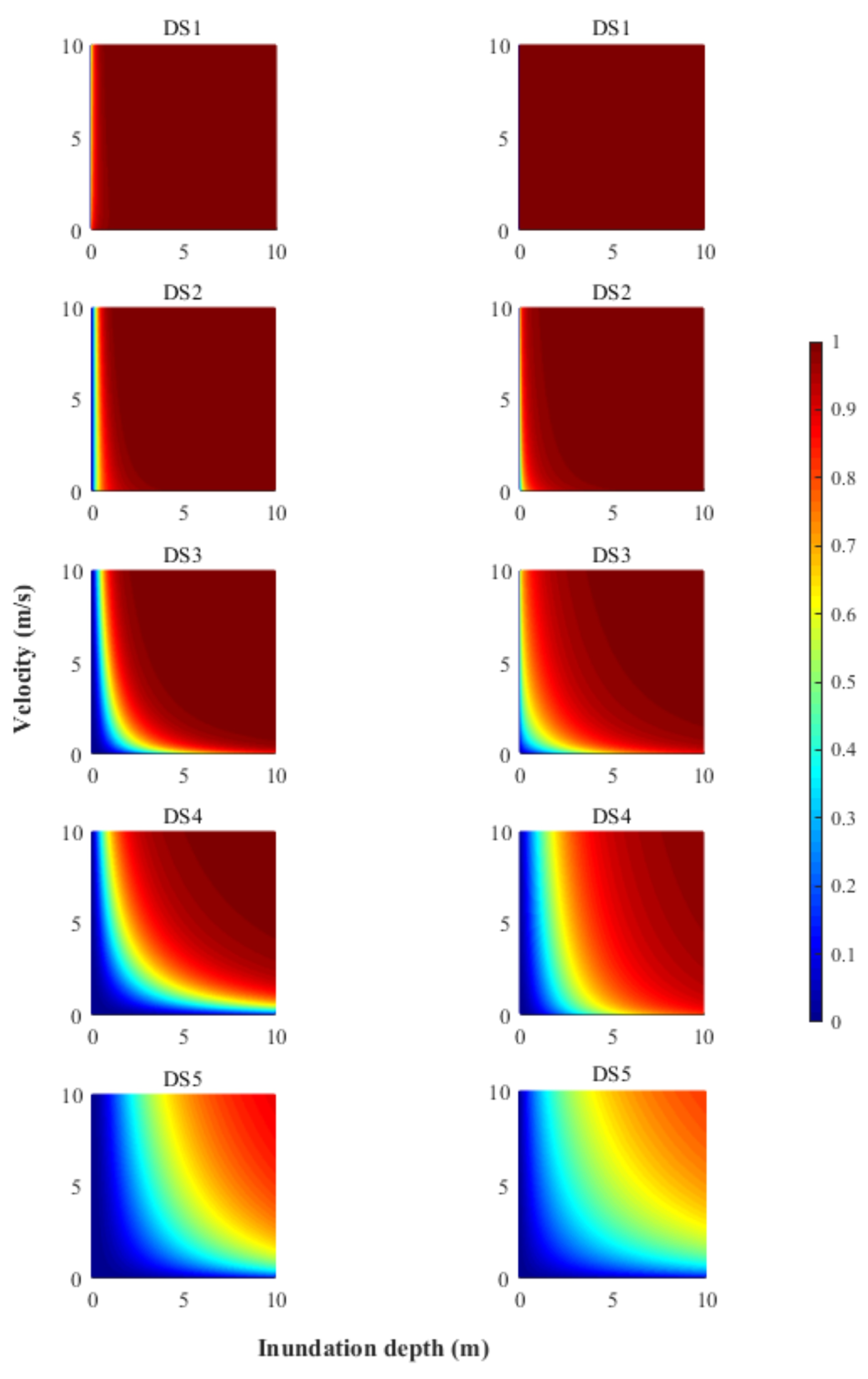
The regression parameters for depth-based fragility according to Equation (6) are shown in Table 1, and Figure 2 shows corresponding fragility curves, noting that this fragility model was referred to as M3 in De Risi et al. [37]. Regression parameters for bivariate-IM fragility according to Equation (7) for plain coast and ria coast are listed in Table 2; this fragility function was referred to as M4 in De Risi et al. [37]. Figure 3 shows an example of bivariate-IM fragility surfaces for RC structures by distinguishing plain and ria coast types. It can be observed that, at higher damage states, the fragility curves are more sensitive to the change of flow velocity. In other words, due to the inclusion of flow velocity, the shape of fragility curves is determined by the velocity. The difference by consideration of velocity is increasing with worsening damage, particularly for DS5 where buildings had collapsed or washed away. Similar fragility surfaces can be obtained for steel, wood and masonry structures.
Integrated with simulated tsunami intensities, for mutually exclusive damage states that are defined in a discrete manner, the damage probability of damage state can be obtained given the IM of a building, which can be expressed as:
Based on the Monte Carlo tsunami simulation results, stochastic tsunami risk for a given region can be obtained for any selected probability levels. By incorporating damage cost models for different buildings, the tsunami damage information can be transformed into tsunami loss information for individual buildings as well as building portfolios. The loss ratios in terms of replacement cost of a building for the six damage levels (i.e., from no damage to collapse & washed-away) can be assigned as: 0.0, 0.05, 0.2, 0.4, 0.6, and 1.0 [41]. Using the damage state probability and the loss ratio , tsunami damage cost for a given tsunami hazard intensity can be calculated as:
where is the replacement cost of a building. An advantage of using loss metrics, instead of damage probability or number of damaged buildings, is that the consequences due to tsunami damage in coastal cities/towns can be aggregated for the entire building portfolio.
Since the MLIT database does not provide occupancy information for individual buildings, the buildings are classified by building materials into residential houses (i.e., wood structures) and commercial buildings (i.e., RC, steel and masonry structures) according to a Japanese building cost information handbook published by the Construction Research Institute [44]. Moreover, typical floor areas of wood-frame houses and store/offices are determined based on the Japan’s national construction statistics maintained by the MLIT [45]. In this study, uncertainty in the cost model is not considered and a mean unit cost and floor area are applied for all buildings. The mean unit cost and mean floor area are 1600 and 130 for residential houses, and 1500 and 540 for commercial buildings. Therefore, the mean replacement cost of a residential house and commercial house is evaluated as 208,000 US$ and 810,000 US$.
2.3. Influence of Flow Velocity on Tsunami Loss
Considering two tsunami intensity measures at the same time in the tsunami fragility, the tsunami loss is evaluated as a function of both inundation depth and flow velocity. The difference in the estimated tsunami loss considering and neglecting flow velocity in terms of all possible combinations of depth and velocity is presented in Figure 4 as the percentage of complete replacement cost, by distinguishing four building materials and two topographical types. The loss is calculated based on the corresponding bivariate-IM fragility of each structural type for a single building and is not related to tsunami hazard results at specific locations. The coloured contour graphs indicate that the importance of flow velocity for the loss estimate largely depends on the local inundation depth and flow velocity of a building.
For both types of coastal topography, when flow velocity is very small, the consideration of velocity can result in an underestimation of tsunami loss. It is noteworthy that the top left corners of the contour graphs are less meaningful because it is rare that a location experiences a low inundation depth and high flow velocity (e.g., 1 m inundation depth with 8 m/s velocity). For the areas where depth-based loss is less than depth–velocity-based loss, the most loss difference occurs in a range of low inundation depth less than 3 m. Although red-coloured and orange-coloured areas for all four structural types are roughly a wedge shape that extends with the increase of flow velocity, given the range of inundation depth of 1 m to 3 m where the largest difference is found, a high velocity such as 8 m/s is not very likely to happen. Moreover, RC structures are the most sensitive to flow velocity with larger areas in red and orange, which cover the combination of an inundation depth higher than 2 m and flow velocity faster than 3 m/s. In other words, for an area that is severely inundated where high flow velocities and high inundation depths are expected, the consideration flow velocity does not make a significant difference compared to a less destructive tsunami.
However, the distributions of tsunami loss considering and neglecting flow velocity for plain coast and ria coast are still slightly different for certain depth–velocity combinations. Firstly, focusing on the most sensitive RC structures, there is a wider gap of green and blue along the velocity axis of the graph of plain coast than ria especially in the left bottom corner, which represents less than 10% difference, as seen in Figure 4a. This means flow velocity is not important when tsunami hazard intensity falls in the range of inundation depth less than 1 m and velocity less than 2.5 m/s for plain coast. This characteristic is not reflected for ria coast shown in Figure 4b. For ria coast, the bivariate-IM fragility produces greater tsunami loss from a velocity value as low as 1 m/s, while this number for plain coast is about 4 m/s. Similar features are found for steel and masonry structures. Secondly, although the region corresponding to a difference between 5% to 30% for RC is roughly the same for plain coast and ria coast, a positive difference for ria coast is found from lower velocity and inundation depth, while that for plain coast occurs only when inundation depth is greater than approximately 2 m and velocity is larger than about 4 m/s. Given a limit of velocity up to 10 m/s, the positive difference for plain coast covers a range of higher inundation depth than ria coast. For all structural types, consideration of velocity results in more tsunami loss from lower velocity values for ria coast than plain coast. A similarity is that, for both topographic types, the loss difference of more than 20% caused by consideration of velocity mainly occurs when inundation depth is lower than 3 m, and it increases with the rise of velocity. Except for RC structures, ria coast has a larger region of difference ratio over 30% than plain coast, particularly for steel and masonry structures. For instance, for masonry, when inundation depth falls between 1 m and 2 m and flow velocity ranges between 3 m/s and 5 m/s, the difference for plain coast is about 5% to 10%, while that for ria coast is 20% to 30%. Judging from the areas of loss difference ratio, RC is the most sensitive to consideration of flow velocity, followed by steel and masonry structures, and wood structures are the least sensitive. This is consistent with general observations of tsunami fragility of wood structures that when the inundation depth reaches a certain value, it tends to be critical regardless of flow velocity. Overall, the importance of flow velocity increases with the increase of flow velocity, however, it is only true for a certain range of inundation depth values.
3. Results and Discussion
Sendai and Onagawa in Miyagi Prefecture are selected as representative locations for plain and ria coast, respectively. Tsunami losses considering and neglecting velocity are compared at three scales: (i) the whole city; (ii) a small community; and (iii) within 1 km from the coastline. The influence of DEM resolution is also considered.
3.1. Sendai
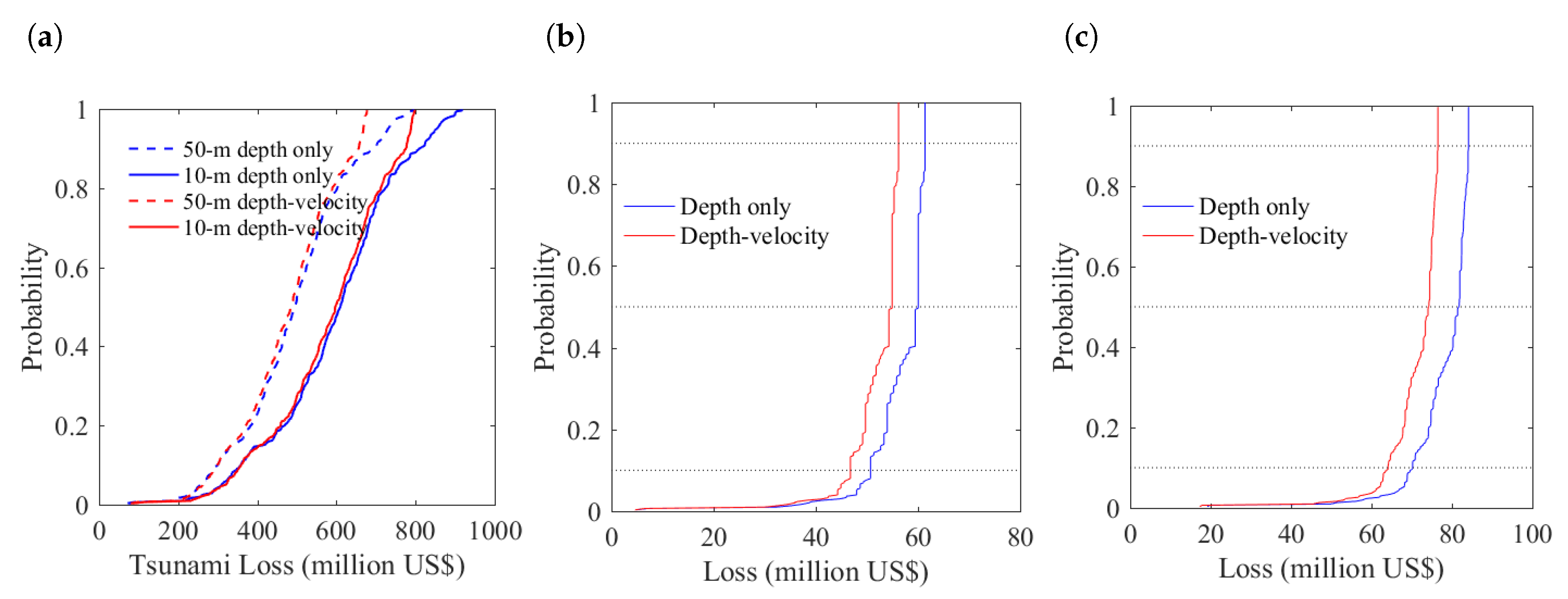
A pre-2011 building portfolio of Sendai consists of 337 RC structures, 695 steel structures, 7488 wood structures, and 1097 masonry structures (Figure 5a). The probabilistic tsunami loss curves for the entire portfolio in Sendai shown in Figure 6a indicate that velocity is not important at a city scale. However, this is the result of the fact that the majority of buildings in Sendai are wood structures that are least sensitive to velocity. Resolution makes a larger difference than consideration of velocity for all of Sendai, with 50-m DEM resulting in more than 20% overestimation in comparison with 10-m resolution. The reason is that, on plain coast, the coarse resolution is unable to reflect the rapid drop of tsunami waves travelling inland realistically.
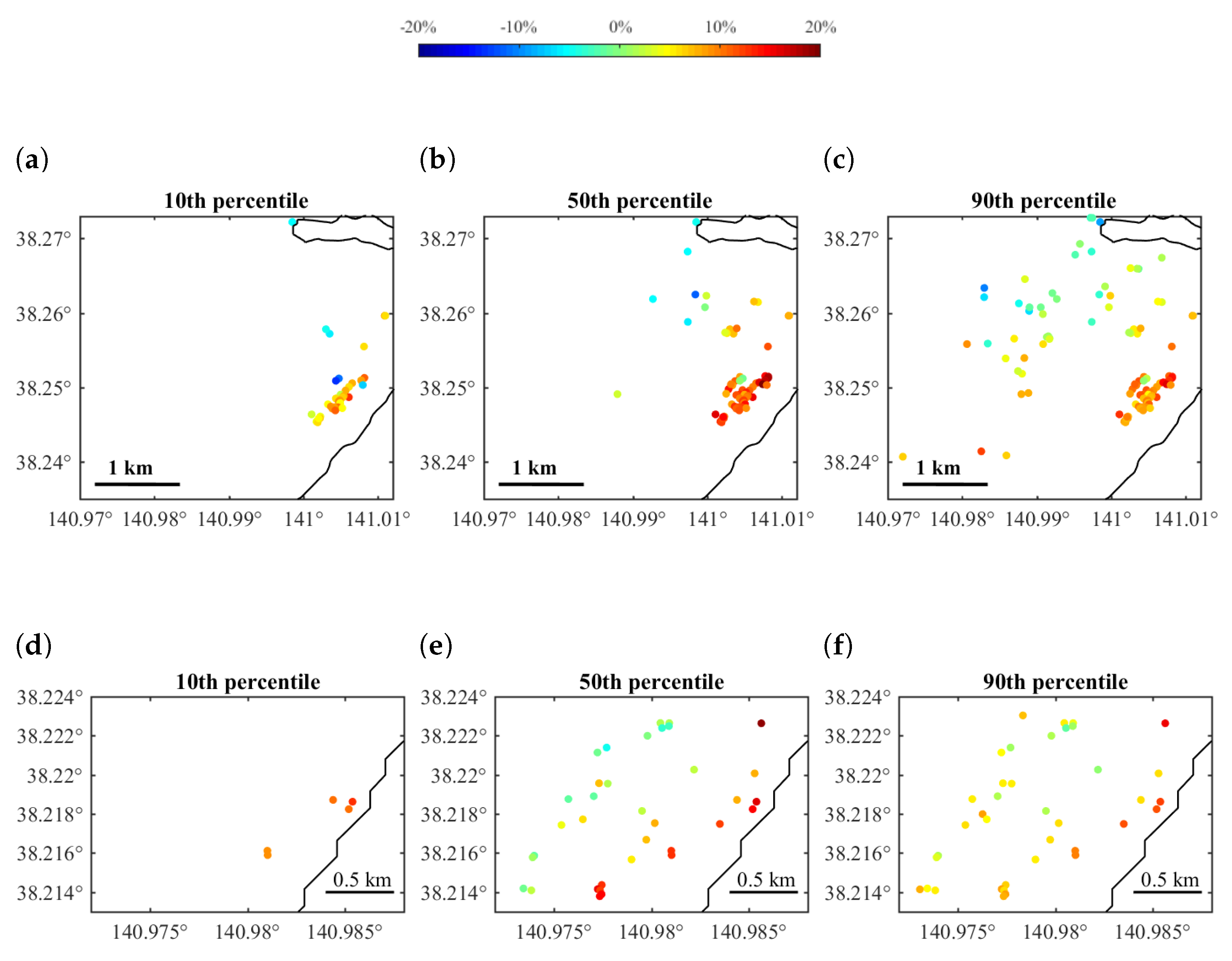
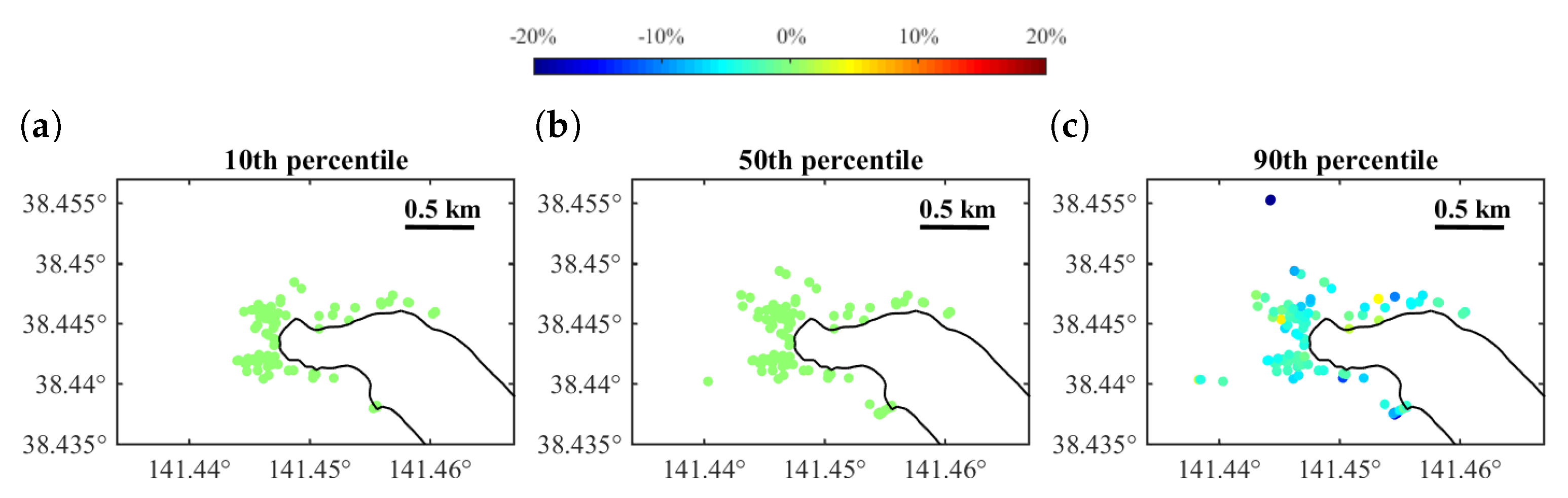
To look into the loss difference more closely, the spatial distribution of differences in the tsunami loss whether velocity is considered for a smaller region R1 for tsunami scenarios corresponding to 10th, 50th and 90th percentiles of total tsunami loss (Figure 7a–c). RC structures are taken for illustration as they are the most sensitive structural type to flow velocity as found in Section 2.3. A positive loss ratio means that flow velocity gives higher loss and a negative one means the opposite. The largest difference occurs at buildings closest to the sea (i.e., within 1 km from the coastline), which experience much faster tsunami flow than the rest of the buildings. It is noteworthy that the difference for this small group of buildings at the 50th percentile is larger than those at the 10th percentile and the 90th percentile. The reason is that the corresponding inundation depths for those buildings at the 90th percentile of total tsunami loss are higher than that at the 50th percentile, while velocities at the 50th percentile are larger than those at the 90th percentile. In addition, the loss difference becomes smaller when inundation depth becomes higher and flow velocity becomes lower, as shown in Figure 4. Such features that the largest difference for certain buildings do not necessarily occur at the high percentiles are caused by the tsunami propagation path of specific scenarios and the location of buildings. To put in another way, the tsunami loss of a small coastal community cannot represent the damage scale of the whole city. Moreover, minor underestimation of bivariate-IM loss is observed at the far end of the building stock. Because both depth and velocity decrease when tsunami waves travel further inland, these buildings fall into the blue area in Figure 4, which means that consideration of velocity generates lower tsunami loss than neglecting it.
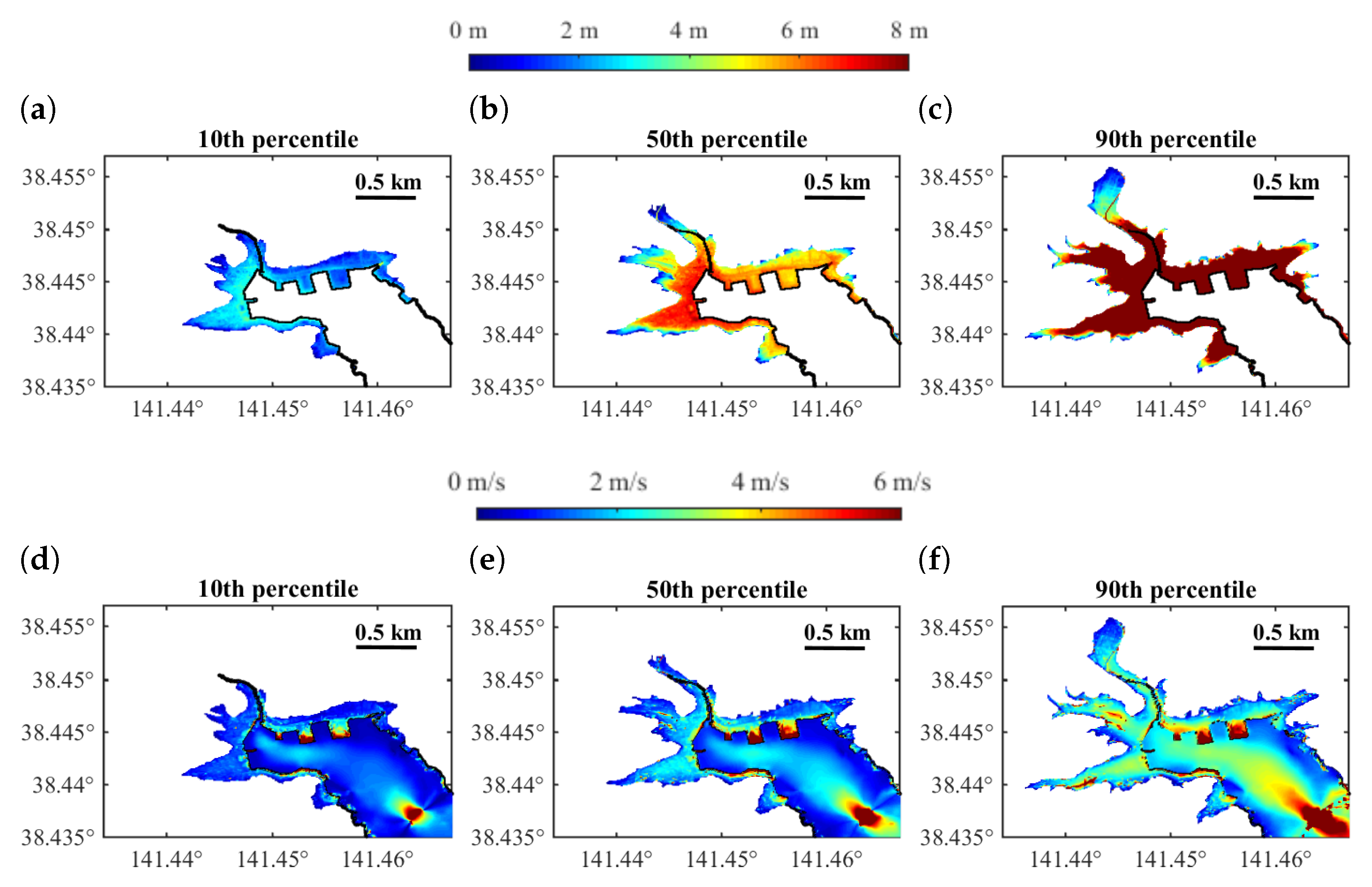
Given the tsunami losses of every building considering and neglecting flow velocity, the percentage of loss difference (i.e., loss considering velocity minus loss neglecting velocity) over total replacement cost was calculated. Since the loss difference distribution in region R1 indicates that buildings located close to the coastline tend to be more sensitive to flow velocity, a small region R2, which is a community located within 1 km from the sea, is focused on, as shown in Figure 5a. Similar features as found in region R1 in terms of largest difference can be seen in region R2 (Figure 7d–f). Overall, the difference is decreased with the increasing distance from the shoreline. Referring to the inundation depth and velocity contour maps in Figure 8, the inundation depth is consistent with the rank of total loss, while higher velocity occurs at the 50th percentile rather than the 90th percentile. It means that, for the same location, a higher inundation does not necessarily comes with a higher velocity for different tsunami scenarios. This also explains why a larger difference is found at the 50th percentile than the 90th percentile. This finding indicates that observations of tsunami hazard level at certain points may not be sufficient to reflect the overall inundation scale. As a result, the actual tsunami propagation inland can make a significant difference in total tsunami loss. In addition, in region R2, no significant underestimation of loss by consideration of velocity is found. Therefore, the importance of flow velocity for tsunami loss estimation in Sendai on plain coast largely depends on the combination of inundation depth and flow velocity of the specific tsunami scenario at buildings’ locations. The depth–velocity distributions of region R2 at three percentile levels shown in Figure 9 indicate that at all three percentiles the majority of inundated buildings fall in the green area, which represents a difference of less than 10%, and a few of them fall into the yellow area, which corresponds to a difference of 10% to 20%.
The sensitivity of RC structures to velocity in region R2 is consistent with the findings in R1. The loss curves for RC buildings in region R2 (Figure 6b) show a more than 10% loss by consideration of flow velocity, which is due to a high proportion of RC buildings being located close to the shoreline (i.e., less than 0.5 km). Another noteworthy feature of tsunami loss curves in region R2 is that the curves start to become steeper after about the 60th percentile. Given the location of region R2 as a small community, when the hazard intensity reaches a certain level, the majority of buildings will collapse or be washed away and thus the increase of tsunami intensity will greatly increase the tsunami loss. This information not only provides potential economic loss for a given building portfolio considering all possible situations, but also indicates the area where the greatest loss comes from. Although corresponding maps based on depth-based fragility can be obtained, for the purpose of exploring the difference caused by flow velocity, the difference between losses based on the bivariate-IM method and the single-IM method is computed and discussed.
Based on the finding above that buildings located within 1 km from the coastline are most sensitive to inclusion of flow velocity in terms of tsunami loss, the tsunami loss curves in Figure 6c show that a loss of up to 15% more is caused by consideration of velocity for buildings within 1 km from the coastline. Although velocity hardly has any influence on tsunami loss of all of Sendai, it does not mean it is not important at the municipal scale. For this specific situation of Sendai, the majority of buildings are wood structures and most buildings are located farther than 1 km from coastline, as presented in Figure 5b. Therefore, the importance of velocity for loss estimation depends on the locations of buildings and composition of building materials.
3.2. Onagawa
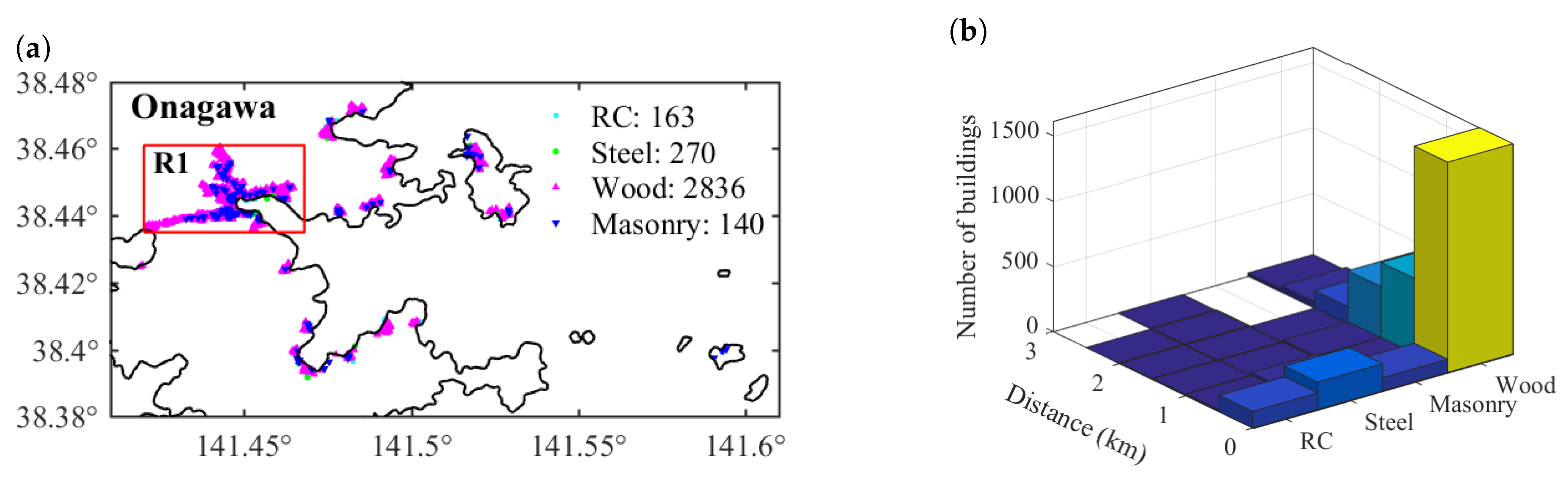
The buildings in Onagawa are distributed along the dendritic shoreline, consisting 163 RC structures, 270 steel structures, 2836 wood structures, and 140 masonry structures. Most buildings are concentrated in region R1, as shown in Figure 10a. A notable feature of the building composition in Onagawa is that most buildings are located within 0.5 km from the coastline where the land is flat (Figure 10b). An opposite finding compared to the results in Sendai in terms of influence of DEM resolution is that the coarse resolution tends to underestimate tsunami loss in Onagawa (Figure 11a). This is due to the rising elevation of Onagawa, and the DEM of coarse resolution cannot accurately simulate the tsunami intensity where the elevation changes abruptly. Although the importance of velocity at a city scale agrees with the finding in Sendai, a deviation is seen above the 90th percentile that consideration of velocity leads to smaller tsunami loss. Another opposite trend of tsunami loss curve of Onagawa compared to that of Sendai is that tsunami loss considering velocity is slightly lower than that neglecting velocity, although the difference is fairly small.
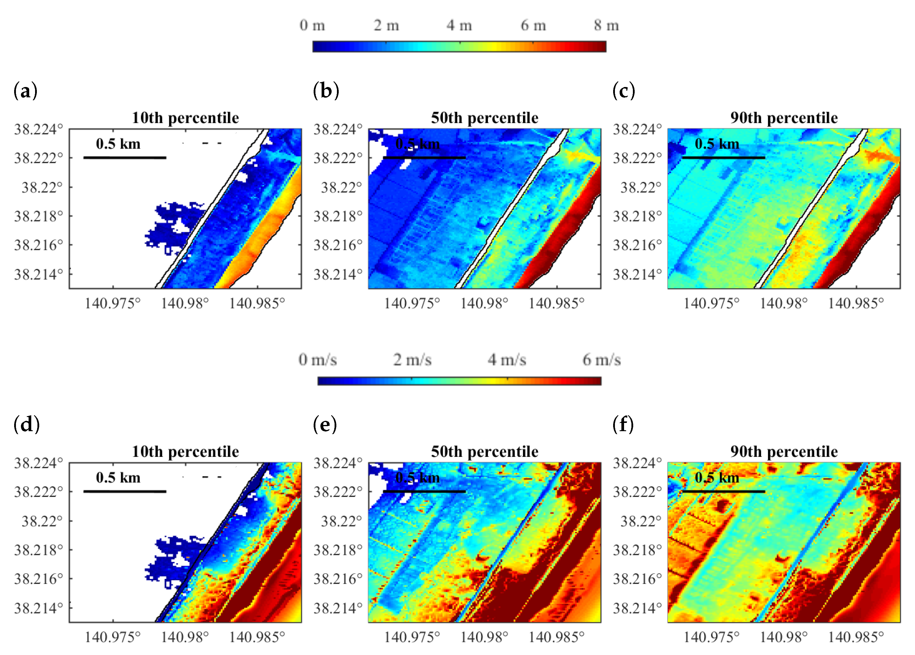
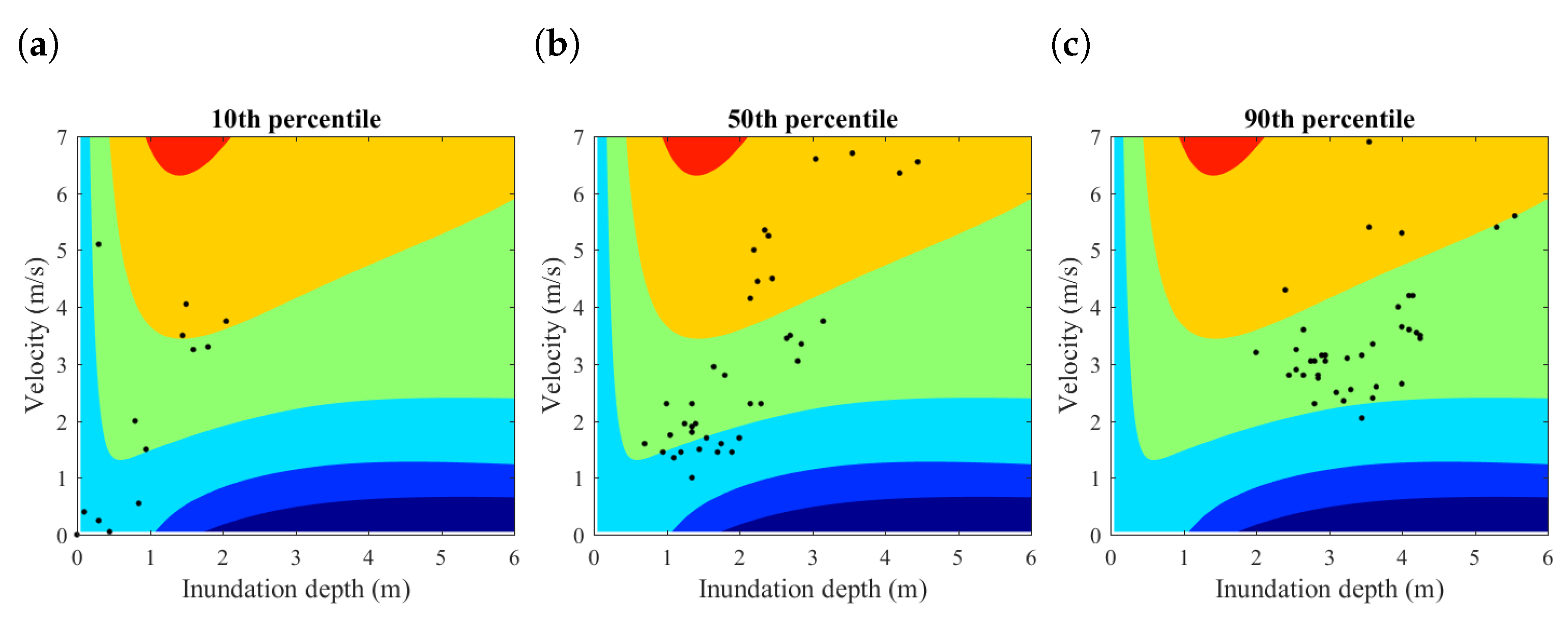
Focusing on region R1 and taking RC structures as an example, Figure 12 shows a significantly different inundation depth–velocity distribution characteristic compared to Sendai on plain coast in which buildings in Onagawa tend to experience low flow velocity with high inundation depth, which agrees with observations [46]. For buildings on ria coast, there are blue strips along the inundation depth axis, and the paired inundation depth and flow velocity in Onagawa make most buildings fit into the green or blue areas, which indicate less than 10% loss difference. The loss difference distribution of RC structures shown in Figure 13 agrees with the loss curves that little difference is found for scenarios corresponding to 10th and 50th percentiles of total loss, whereas underestimation of less than 5%, which is caused by flow velocity, is seen at the 90th percentile. Not many RC buildings experience flow velocity larger than 5 m/s and a concentration of points can be found with inundation depth higher than 10 m, which can also be seen from the inundation maps in Figure 14. These results show the dominating influence of inundation depth on estimated tsunami loss for 9.0 tsunami in Onagawa. However, for RC structures in R1, an approximately 10% difference still exists (Figure 11b) because the majority of RC structures in region R1 fall in the areas which represent difference in Figure 12. Another feature of tsunami loss for buildings in Onagawa is that the probabilistic loss curve becomes very steep after the 10th percentile for RC, which means that the inundation scale in region R1 in Onagawa is more extensive given the same set of tsunami scenarios. This implies that, for tsunamis generated by earthquakes of lower magnitudes, the conclusion may be different because the combination of depth and velocity will be different. Assuming a tsunami of lower earthquake magnitude generates lower inundation depth, the tsunami loss estimation considering flow velocity may not be less than that neglecting flow velocity.
The tsunami loss curves shown in Figure 11c are consistent with the finding for Sendai on plain coast that the buildings close to the coastline are more sensitive to consideration of velocity. This is true for region R1 in Onagawa only because the land is flat for area close to the coastline, and thus may not apply to other cities and towns on ria coast where the features of land elevation are different. Similar to Sendai, consideration of velocity does not make a significant difference in the tsunami loss for all of Onagawa, due to the dominance of wood structures.
Therefore, the importance of flow velocity for ria coast is related to the inundation scale, land elevation, building distributions and building materials.
4. Conclusions
This paper investigated the importance of flow velocity, in addition to inundation depth, to tsunami loss estimation at different scales, by distinguishing plain and ria coastal types. The main conclusions are:
- Tsunami losses of both Sendai on plain coast and Onagawa on ria coast are highly sensitive to DEM resolution. In addition, 50-m DEM gives 20% more loss for Sendai and 20% less loss in Onagawa than 10-m DEM. DEM of coarse resolution is unable to realistically reflect the gradually decaying tsunami waves over inland and the change of land elevation.
- For both plain and ria coasts, RC buildings are the most sensitive structure type to flow velocity, followed by steel and masonry. Wood structures are not sensitive to consideration of velocity for tsunami loss estimation.
- The importance of flow velocity for tsunami mainly depends on the inundation depth and flow velocity combinations at buildings’ locations. Velocity is more important for buildings located close to the sea (e.g., less than 1 km). The influence of velocity for total tsunami loss at a municipal or community scale, depends on the locations of buildings, the main structural types, topography, land elevation, and inundation scale. For buildings located close to the sea affected by a small tsunami and buildings located farther from the shoreline affected by a destructive tsunami, flow velocity may be important for more accurate loss estimation, but for buildings close to the sea due to a destructive tsunami, flow velocity may not be important. However, for a 9.0 Tohoku-type tsunami, loss estimation for buildings located very close to the sea is more likely to be influenced by the inclusion of flow velocity.
Supplementary Materials
Supporting data are provided as supplementary information. Figures for colour blinded readers are available from the Figshare database, under the DOI: http://dx.doi.org/10.6084/m9.figshare.5545645.
Acknowledgments
The bathymetry and elevation data for the Tohoku region were provided by the Miyagi Prefectural Government. The tsunami damage data for the 2011 Tohoku earthquake were obtained from the Ministry of Land, Infrastructure, and Transportation (http://www.mlit.go.jp/toukeijouhou/chojou/stat-e.htm). This work is funded by the Engineering and Physical Sciences Research Council (EP/M001067/1).
Author Contributions
All authors contributed to the paper. J.S. took the leadership in conducting numerical calculations and producing the main results, whereas R.D.R. and K.G. supported J.S. in carrying out tsunami fragility analysis and tsunami loss estimation. All authors have reviewed and approved the content of this paper.
Conflicts of Interest
The authors declare no conflict of interest.
Abbreviations
The following abbreviations are used in this manuscript:
| DEM | Digital Elevation Model |
| MLIT | Ministry of Land, Infrastructure, and Transportation |
| h | Inundation depth |
| v | Flow velocity |
| Momentum flux | |
| MLE | Maximum likelihood estimation |
References
- Mitchell-Wallace, K.; Foote, M.; Jones, M.; Hillier, J. Natural Catastrophe Risk Management and Modelling: A Practitioner’s Guide; John Wiley & Sons: Hoboken, NJ, USA, 2017. [Google Scholar]
- Lakdawalla, D.; Zanjani, G. Catastrophe bonds, reinsurance, and the optimal collateralization of risk transfer. J. Risk Insur. 2012, 79, 449–476. [Google Scholar] [CrossRef]
- Gibson, R.; Habib, M.A.; Ziegler, A. Reinsurance or securitization: The case of natural catastrophe risk. J. Math. Econ. 2014, 53, 79–100. [Google Scholar] [CrossRef] [Green Version]
- Yoshikawa, H.; Goda, K. Financial seismic risk analysis of building portfolios. Nat. Hazards Rev. 2013, 15, 112–120. [Google Scholar] [CrossRef]
- Hagendorff, B.; Hagendorff, J.; Keasey, K.; Gonzalez, A. The risk implications of insurance securitization: The case of catastrophe bonds. J. Corp. Financ. 2014, 25, 387–402. [Google Scholar] [CrossRef] [Green Version]
- Goda, K. Seismic risk management of insurance portfolio using catastrophe bonds. Comput. Civ. Infrastruct. Eng. 2015, 30, 570–582. [Google Scholar] [CrossRef]
- Park, H.; Cox, D.T.; Barbosa, A.R. Comparison of inundation depth and momentum flux based fragilities for probabilistic tsunami damage assessment and uncertainty analysis. Coast. Eng. 2017, 122, 10–26. [Google Scholar] [CrossRef]
- Macabuag, J.; Rossetto, T.; Ioannou, I.; Suppasri, A.; Sugawara, D.; Adriano, B.; Imamura, F.; Eames, I.; Koshimura, S. A proposed methodology for deriving tsunami fragility functions for buildings using optimum intensity measures. Nat. Hazards 2016, 84, 1257–1285. [Google Scholar] [CrossRef]
- Suppasri, A.; Mas, E.; Charvet, I.; Gunasekera, R.; Imai, K.; Fukutani, Y.; Abe, Y.; Imamura, F. Building damage characteristics based on surveyed data and fragility curves of the 2011 Great East Japan tsunami. Nat. Hazards 2013, 66, 319–341. [Google Scholar] [CrossRef]
- Charvet, I.; Ioannou, I.; Rossetto, T.; Suppasri, A.; Imamura, F. Empirical fragility assessment of buildings affected by the 2011 Great East Japan tsunami using improved statistical models. Nat. Hazards 2014, 73, 951–973. [Google Scholar] [CrossRef]
- Narita, Y.; Koshimura, S. Classification of tsunami fragility curves based on regional characteristics of tsunami damage. J. Jpn. Soc. Civ. Eng. Ser. B2 Coast. Eng. 2015, 71, I_331–I_336. (In Japnese) [Google Scholar] [CrossRef]
- De Risi, R.; Goda, K.; Mori, N.; Yasuda, T. Bayesian tsunami fragility modeling considering input data uncertainty. Stoch. Environ. Res. Risk Assess. 2017, 31, 1253–1269. [Google Scholar] [CrossRef]
- Yeh, H.; Sato, S.; Tajima, Y. The 11 March 2011 East Japan earthquake and tsunami: Tsunami effects on coastal infrastructure and buildings. Pure Appl. Geophys. 2013, 170, 1019–1031. [Google Scholar] [CrossRef]
- Yeh, H.; Barbosa, A.R.; Ko, H.; Cawley, J. Tsunami loadings on structures: Review and analysis. Coast. Eng. Proc. 2014, 1, 1–13. [Google Scholar] [CrossRef]
- Fritz, H.; Borrero, J.; Synolakis, C.; Yoo, J. 2004 Indian Ocean tsunami flow velocity measurements from survivor videos. Geophys. Res. Lett. 2006, 33. [Google Scholar] [CrossRef]
- Hayashi, S.; Koshimura, S. The 2011 Tohoku tsunami flow velocity estimation by the aerial video analysis and numerical modeling. J. Disaster Res. 2013, 8, 561–572. [Google Scholar] [CrossRef]
- Lipa, B.; Isaacson, J.; Nyden, B.; Barrick, D. Tsunami arrival detection with high frequency (HF) radar. Remote Sens. 2012, 4, 1448–1461. [Google Scholar] [CrossRef]
- Song, Y.T.; Fukumori, I.; Shum, C.K.; Yi, Y. Merging tsunamis of the 2011 Tohoku-Oki earthquake detected over the open ocean. Geophys. Res. Lett. 2012, 39. [Google Scholar] [CrossRef]
- Charvet, I.; Suppasri, A.; Kimura, H.; Sugawara, D.; Imamura, F. A multivariate generalized linear tsunami fragility model for Kesennuma City based on maximum flow depths, velocities and debris impact, with evaluation of predictive accuracy. Nat. Hazards 2015, 79, 2073–2099. [Google Scholar] [CrossRef]
- Koshimura, S.; Oie, T.; Yanagisawa, H.; Imamura, F. Developing fragility functions for tsunami damage estimation using numerical model and post-tsunami data from Banda Aceh, Indonesia. Coast. Eng. J. 2009, 51, 243–273. [Google Scholar] [CrossRef]
- Maruyama, Y.; Kitamura, K.; Yamazaki, F. Tsunami damage assessment of buildings in Chiba Prefecture, Japan using fragility function developed after the 2011 Tohoku-Oki Earthquake. In Safety, Reliability, Risk and Life-Cycle Performance of Structures and Infrastructures; Taylor & Francis Group: London, UK, 2013; pp. 4237–4244. [Google Scholar]
- Tanaka, N.; Onai, A.; Kondo, K. Fragility curve of different damage of wooden building due to tsunami based on tsunami fluid force and its moment. J. Jpn. Soc. Civ. Eng. Coast. Eng. 2015, 71, 1–11. [Google Scholar] [CrossRef]
- Park, H.; Cox, D.T. Probabilistic assessment of near-field tsunami hazards: Inundation depth, velocity, momentum flux, arrival time, and duration applied to Seaside, Oregon. Coast. Eng. 2016, 117, 79–96. [Google Scholar] [CrossRef]
- González-Riancho, P.; Aguirre-Ayerbe, I.; García-Aguilar, O.; Medina, R.; González, M.; Aniel-Quiroga, I.; Gutiérrez, O.Q.; Álvarez-Gómez, J.A.; Larreynaga, J.; Gavidia, F. Integrated tsunami vulnerability and risk assessment: Application to the coastal area of El Salvador. Nat. Hazards Earth Syst. Sci. 2014, 14, 1223–1244. [Google Scholar] [CrossRef] [Green Version]
- Schneider, B.; Hoffmann, G.; Reicherter, K. Scenario-based tsunami risk assessment using a static flooding approach and high-resolution digital elevation data: An example from Muscat in Oman. Glob. Planet. Chang. 2016, 139, 183–194. [Google Scholar] [CrossRef]
- Browning, J.; Thomas, N. An assessment of the tsunami risk in Muscat and Salalah, Oman, based on estimations of probable maximum loss. Int. J. Disaster Risk Reduct. 2016, 16, 75–87. [Google Scholar] [CrossRef]
- Okumura, N.; Jonkman, S.N.; Esteban, M.; Hofland, B.; Shibayama, T. A method for tsunami risk assessment: A case study for Kamakura, Japan. Nat. Hazards 2017, 88, 1451–1472. [Google Scholar] [CrossRef]
- Goda, K.; Mai, P.M.; Yasuda, T.; Mori, N. Sensitivity of tsunami wave profiles and inundation simulations to earthquake slip and fault geometry for the 2011 Tohoku earthquake. Earth Planets Space 2014, 66, 1–20. [Google Scholar] [CrossRef] [Green Version]
- Mueller, C.; Power, W.; Fraser, S.; Wang, X. Effects of rupture complexity on local tsunami inundation: Implications for probabilistic tsunami hazard assessment by example. J. Geophys. Res. Solid Earth 2015, 120, 488–502. [Google Scholar] [CrossRef]
- Goda, K.; Abilova, K. Tsunami hazard warning and risk prediction based on inaccurate earthquake source parameters. Nat. Hazards Earth Syst. Sci. 2016, 16, 577–593. [Google Scholar] [CrossRef]
- Goda, K.; Song, J. Uncertainty modeling and visualization for tsunami hazard and risk mapping: A case study for the 2011 Tohoku earthquake. Stoch. Environ. Res. Risk Assess. 2016, 30, 2271–2285. [Google Scholar] [CrossRef] [Green Version]
- Jaimes, M.A.; Reinoso, E.; Ordaz, M.; Huerta, B.; Silva, R.; Mendoza, E.; Rodríguez, J.C. A new approach to probabilistic earthquake-induced tsunami risk assessment. Ocean Coast. Manag. 2016, 119, 68–75. [Google Scholar] [CrossRef]
- Goda, K.; Yasuda, T.; Mori, N.; Maruyama, T. New Scaling Relationships of Earthquake Source Parameters for Stochastic Tsunami Simulations. Coast. Eng. J. 2016, 58, 1–40. [Google Scholar] [CrossRef]
- Murotani, S.; Satake, K.; Fujii, Y. Scaling relations of seismic moment, rupture area, average slip, and asperity size for M9 subduction-zone earthquakes. Geophys. Res. Lett. 2013, 40, 5070–5074. [Google Scholar] [CrossRef]
- Petrone, C.; Rossetto, T.; Goda, K. Fragility assessment of a RC structure under tsunami actions via nonlinear static and dynamic analyses. Eng. Struct. 2017, 136, 36–53. [Google Scholar] [CrossRef]
- Goto, C.; Ogawa, Y.; Shuto, N. IUGG/IOC Time Project: Numerical Method of Tsunami Simulation with the Leap-Frog Scheme; IOC Manuals and Guides No. 35; UNESCO: Paris, France, 1997. [Google Scholar]
- De Risi, R.; Goda, K.; Yasuda, T.; Mori, N. Is flow velocity important in tsunami empirical fragility modeling? Earth-Sci. Rev. 2017, 166, 64–82. [Google Scholar] [CrossRef]
- Mai, P.M.; Beroza, G.C. A spatial random field model to characterize complexity in earthquake slip. J. Geophys. Res. Solid Earth 2002, 107. [Google Scholar] [CrossRef]
- Mai, P.M.; Thingbaijam, K.K.S. SRCMOD: An online database of finite-fault rupture models. Seismol. Res. Lett. 2014, 85, 1348–1357. [Google Scholar] [CrossRef]
- Satake, K.; Fujii, Y.; Harada, T.; Namegaya, Y. Time and space distribution of coseismic slip of the 2011 Tohoku earthquake as inferred from tsunami waveform data. Bull. Seismol. Soc. Am. 2013, 103, 1473–1492. [Google Scholar] [CrossRef]
- Ministry of Land, Infrastructure and Transportation (MLIT). Survey of Tsunami Damage Condition. Available online: http://www.mlit.go.jp/toshi/toshi-hukkou-arkaibu.html (accessed on 1 July 2014).
- De Risi, R.; Goda, K. Probabilistic earthquake–tsunami multi-hazard analysis: Application to the Tohoku region, Japan. Front. Built Environ. 2016, 2. [Google Scholar] [CrossRef]
- Hosmer, D.W.; Lemeshow, S.; Sturdivant, R.X. Applied Logistic Regression; John Wiley & Sons: Hoboken, NJ, USA, 2013. [Google Scholar]
- Construction Research Institute. Japan Building Cost Information; Construction Research Institute: Tokyo, Japan, 2011. [Google Scholar]
- Ministry of Land, Infrastructure and Transportation (MLIT). Available online: http://www.mlit.go.jp/toukeijouhou/chojou/stat-e.htm (accessed on 1 July 2014).
- Latcharote, P.; Suppasri, A.; Yamashita, A.; Adriano, B.; Koshimura, S.; Kai, Y.; Imamura, F. Possible failure mechanism of buildings overturned during the 2011 Great East Japan tsunami in the town of Onagawa. Front. Built Environ. 2017, 3, 1–18. [Google Scholar] [CrossRef]
Figure 1.
An example of a synthesised earthquake source model.
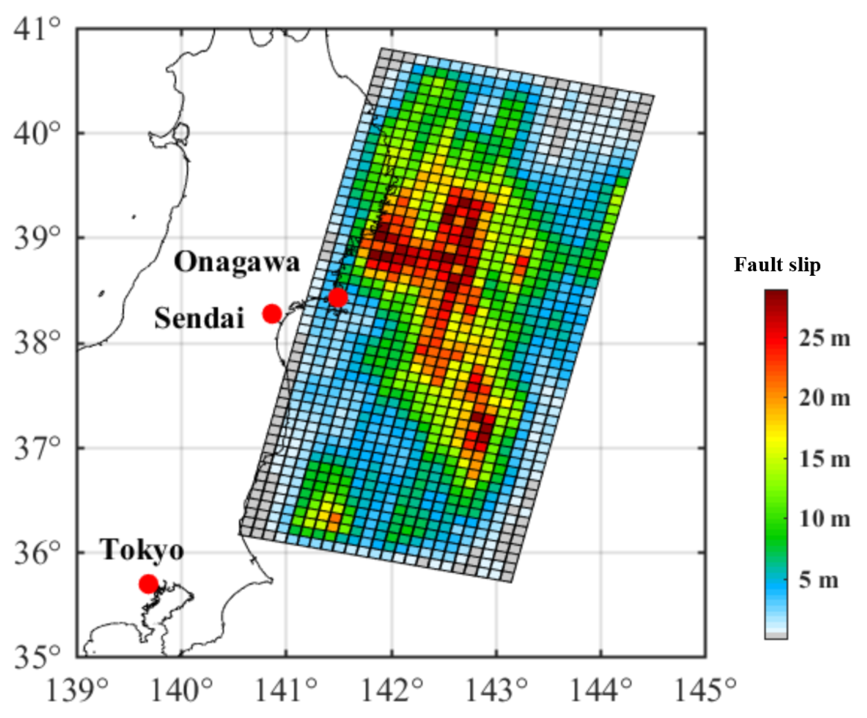
Figure 2.
Fragility neglecting flow velocity for four structural types: (a) RC; (b) steel; (c) wood; and (d) masonry.
Figure 2.
Fragility neglecting flow velocity for four structural types: (a) RC; (b) steel; (c) wood; and (d) masonry.
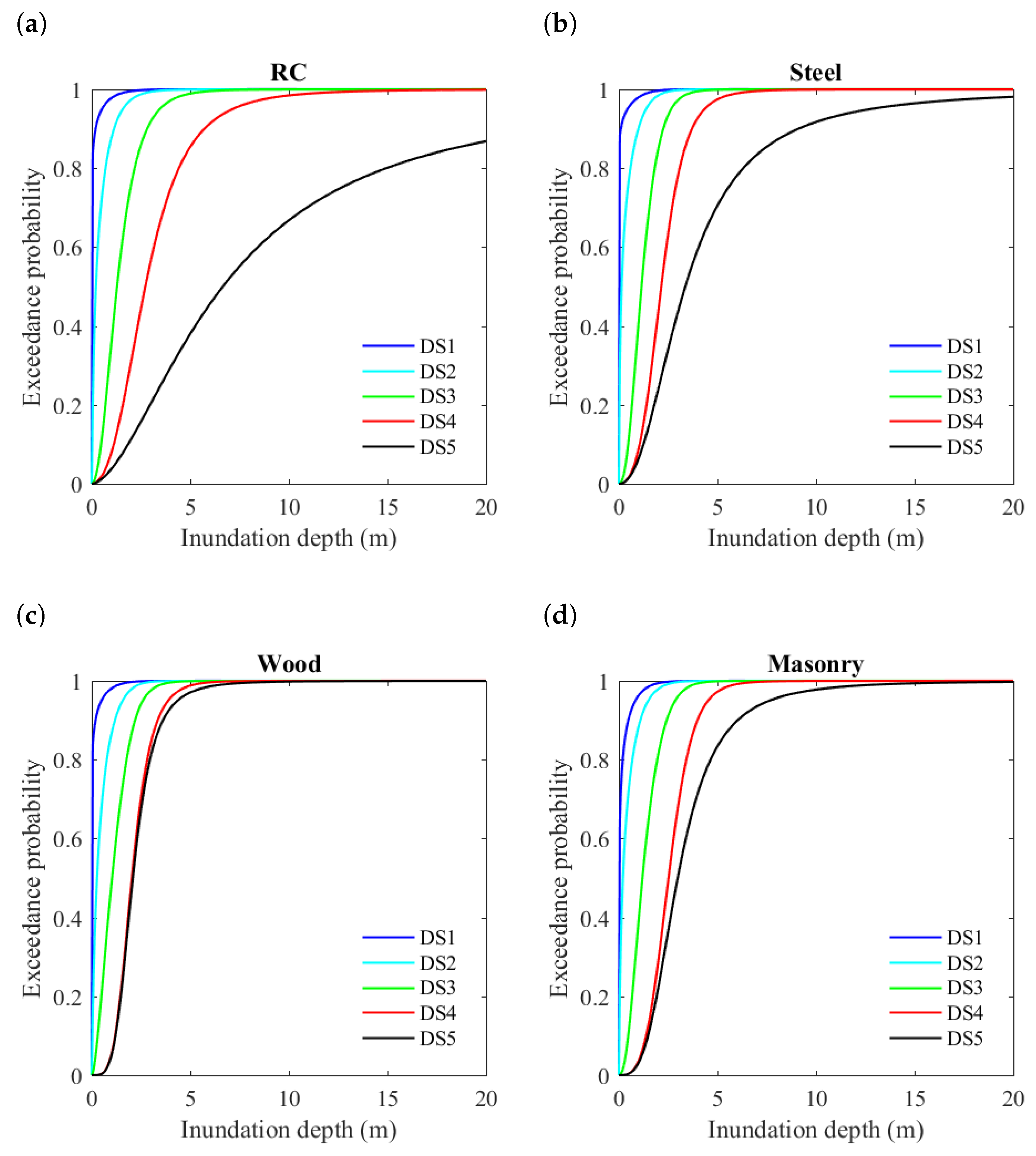
Figure 3.
Fragility surfaces considering flow velocity for RC structures (on the left for plain coast and on the right for ria coast).
Figure 3.
Fragility surfaces considering flow velocity for RC structures (on the left for plain coast and on the right for ria coast).

Figure 4.
Percentage of loss difference considering and neglecting velocity: (a,b) RC; (c,d) steel; (e,f) wood; and (g,h) masonry; on the left for plain coast and on the right for ria coast.
Figure 4.
Percentage of loss difference considering and neglecting velocity: (a,b) RC; (c,d) steel; (e,f) wood; and (g,h) masonry; on the left for plain coast and on the right for ria coast.
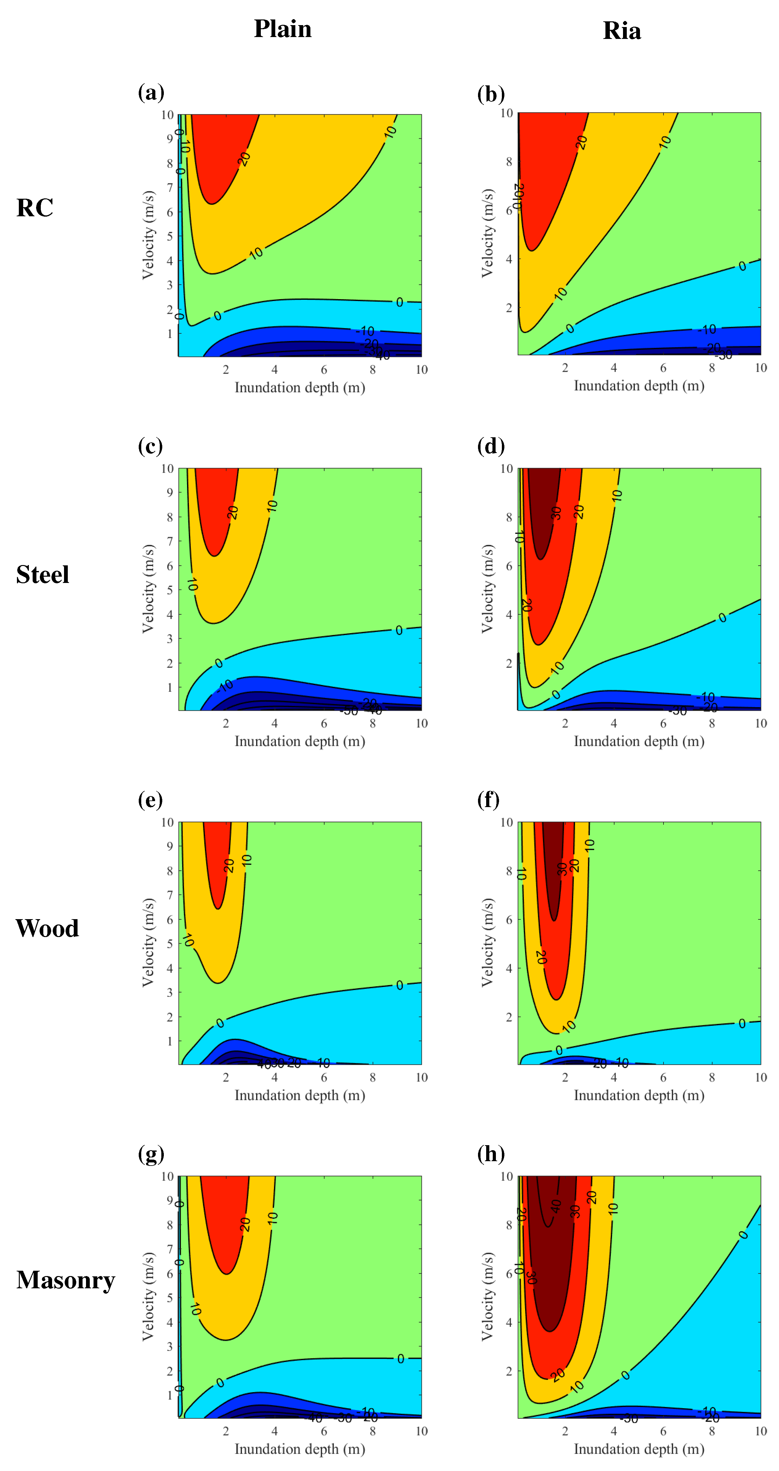
Figure 5.
Building portfolio of Sendai: (a) building distribution; and (b) number of buildings by distance from the coastline.
Figure 5.
Building portfolio of Sendai: (a) building distribution; and (b) number of buildings by distance from the coastline.
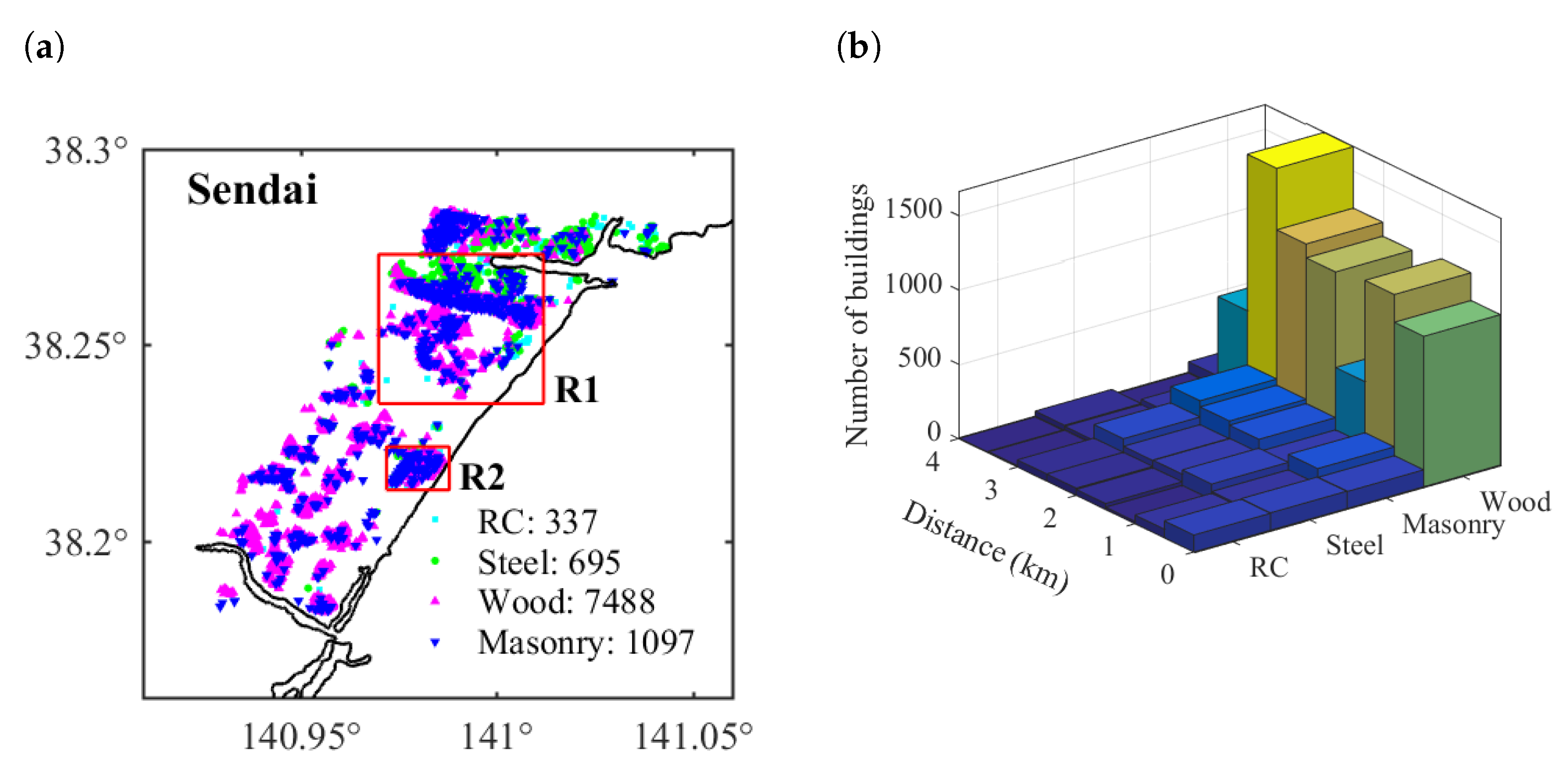
Figure 6.
Probabilistic tsunami loss in Sendai: (a) all of Sendai; (b) RC in region R2; and (c) buildings within 1 km from the coastline.
Figure 6.
Probabilistic tsunami loss in Sendai: (a) all of Sendai; (b) RC in region R2; and (c) buildings within 1 km from the coastline.
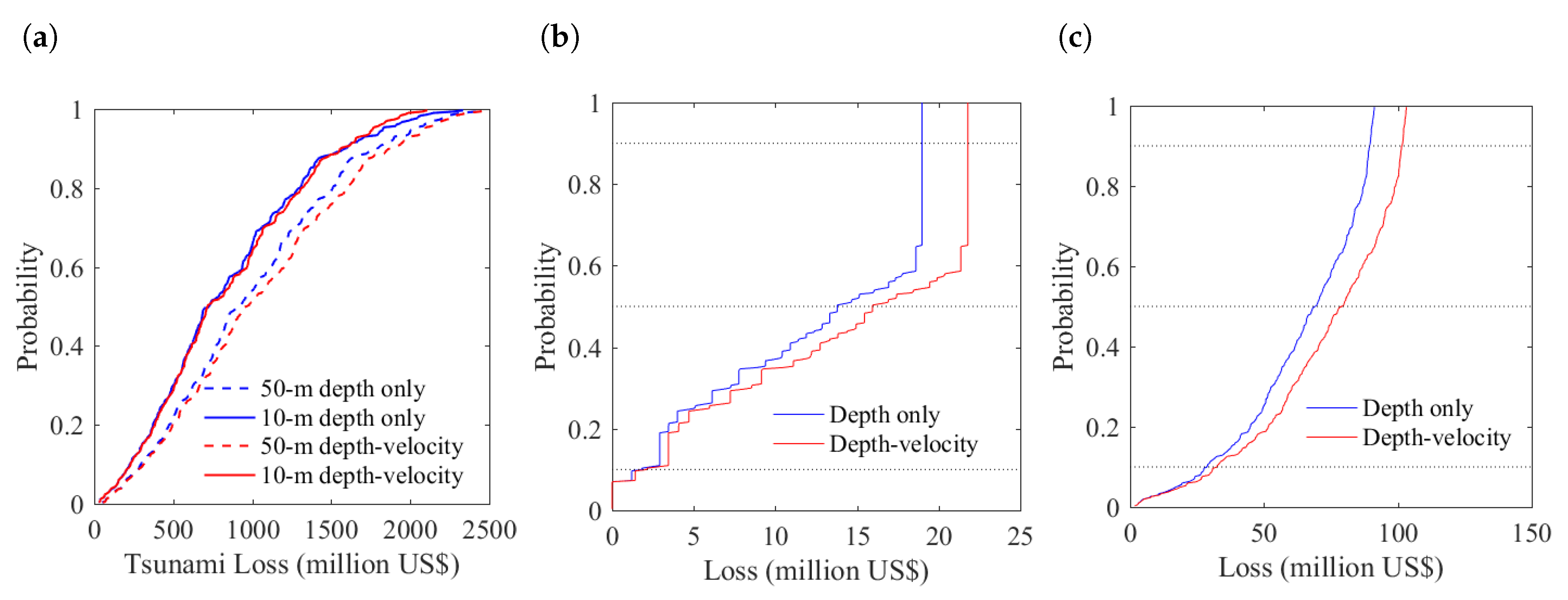
Figure 7.
Distribution of loss difference ratio for RC structures in small regions R1 and R2 of Sendai: (a–c) region R1 and (d–f) region R2.
Figure 7.
Distribution of loss difference ratio for RC structures in small regions R1 and R2 of Sendai: (a–c) region R1 and (d–f) region R2.

Figure 8.
Stochastic tsunami hazard maps for region R2 in Sendai: (a–c) inundation depth; and (d–f) velocity.
Figure 8.
Stochastic tsunami hazard maps for region R2 in Sendai: (a–c) inundation depth; and (d–f) velocity.

Figure 9.
Distribution of inundation depth and flow velocity for RC structures of region R2 in Sendai: (a) 10th percentile; (b) 50th percentile; and (c) 90th percentile.
Figure 9.
Distribution of inundation depth and flow velocity for RC structures of region R2 in Sendai: (a) 10th percentile; (b) 50th percentile; and (c) 90th percentile.

Figure 10.
Building portfolio of Onagawa: (a) building distribution; and (b) number of buildings by distance from the coastline.
Figure 10.
Building portfolio of Onagawa: (a) building distribution; and (b) number of buildings by distance from the coastline.

Figure 11.
Probabilistic tsunami loss in Onagawa: (a) all of Sendai; (b) RC in region R2; and (c) buildings within 1 km from the coastline.
Figure 11.
Probabilistic tsunami loss in Onagawa: (a) all of Sendai; (b) RC in region R2; and (c) buildings within 1 km from the coastline.

Figure 12.
Distribution of inundation depth and flow velocity for RC structures of region R1 in Onagawa: (a) 10th percentile; (b) 50th percentile; and (c) 90th percentile.
Figure 12.
Distribution of inundation depth and flow velocity for RC structures of region R1 in Onagawa: (a) 10th percentile; (b) 50th percentile; and (c) 90th percentile.
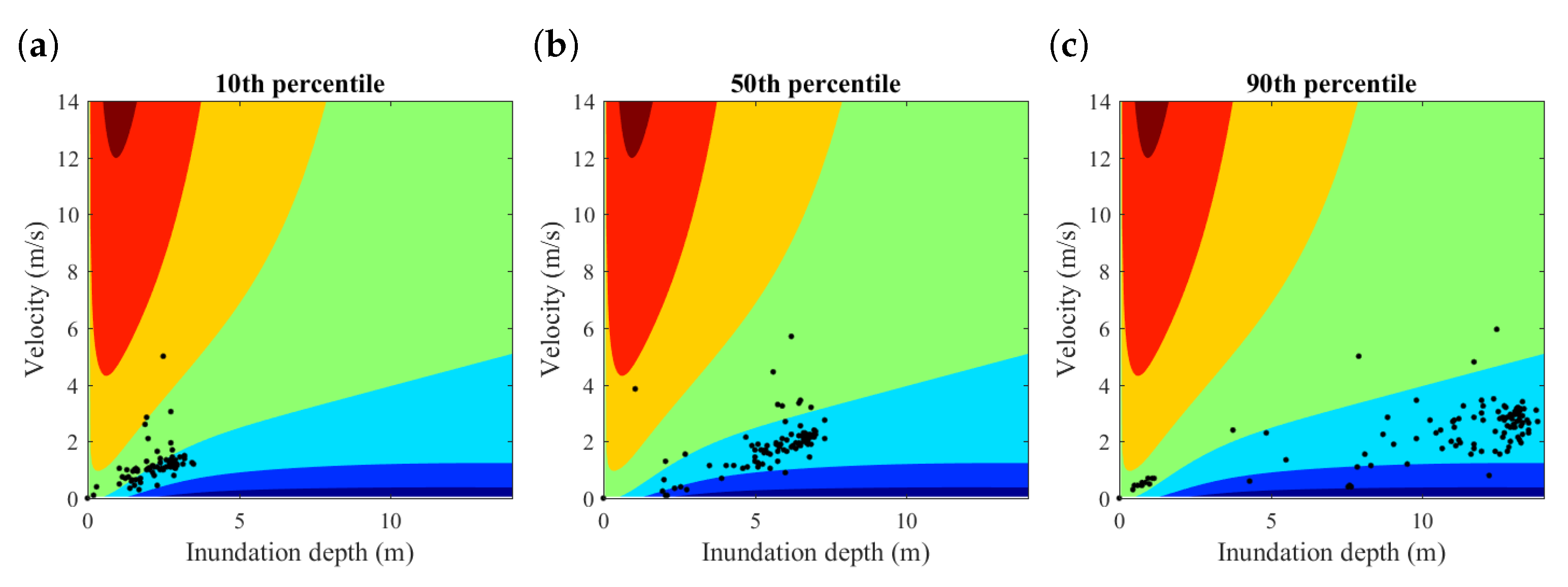
Figure 13.
Distribution of loss difference for RC structures of region R1 in Onagawa: (a) 10th percentile; (b) 50th percentile; and (c) 90th percentile.
Figure 13.
Distribution of loss difference for RC structures of region R1 in Onagawa: (a) 10th percentile; (b) 50th percentile; and (c) 90th percentile.

Figure 14.
Stochastic tsunami hazard maps for region R1 in Onagawa: (a–c) inundation depth; and (d–f) flow velocity.
Figure 14.
Stochastic tsunami hazard maps for region R1 in Onagawa: (a–c) inundation depth; and (d–f) flow velocity.

Table 1.
Regression parameters of single-IM tsunami fragility neglecting flow velocity.
| Parameter | DS1 | DS2 | DS3 | DS4 | DS5 |
|---|---|---|---|---|---|
| 1.54 | 1.43 | ||||
| 0.105 | 0.924 | 1.65 | 2.299 | 1.557 | |
| 0.186 | 0.768 | 0.738 | |||
| 0.023 | 0.437 | 0.215 | |||
| 0.169 | 0.213 | 0.696 | |||
| 0.058 | 0.906 | 2.023 | |||
| 0.108 | 0.27 | 1.486 | 1.16 | ||
| 0.319 | 0.878 | 0.354 |
Table 2.
Regression parameters of bivariate-IM tsunami fragility considering flow velocity.
| Parameter | Plain Coast | Ria Coast | ||||||||
|---|---|---|---|---|---|---|---|---|---|---|
| DS1 | DS2 | DS3 | DS4 | DS5 | DS1 | DS2 | DS3 | DS4 | DS5 | |
| 1.795 | 1.742 | 81.396 | 1.685 | |||||||
| 0.307 | 1.355 | 1.925 | 1.564 | 1.701 | 1.638 | 0.827 | 0.458 | 1.774 | 1.063 | |
| 1.105 | 0.548 | 0.459 | 0.432 | |||||||
| 0.754 | 0.144 | 105.544 | 0.767 | 1.039 | ||||||
| 0.406 | 0.589 | 21.37 | 0.223 | 0.486 | 0.849 | |||||
| 1.415 | 2.001 | 0.052 | 0.976 | 1.47 | 2.491 | |||||
| 0.375 | 1.263 | 0.088 | 0.808 | 2.09 | 0.595 | |||||
| 1.152 | 0.296 | 0.776 | 0.702 | 1.73 | 0.304 | |||||
| 0.782 | 1.604 | 0.850 | 0.004 | 0.767 | 0.234 | 0.773 | ||||
© 2017 by the authors. Licensee MDPI, Basel, Switzerland. This article is an open access article distributed under the terms and conditions of the Creative Commons Attribution (CC BY) license (http://creativecommons.org/licenses/by/4.0/).
Share and Cite
MDPI and ACS Style
Song, J.; De Risi, R.; Goda, K. Influence of Flow Velocity on Tsunami Loss Estimation. Geosciences 2017, 7, 114. https://doi.org/10.3390/geosciences7040114
AMA Style
Song J, De Risi R, Goda K. Influence of Flow Velocity on Tsunami Loss Estimation. Geosciences. 2017; 7(4):114. https://doi.org/10.3390/geosciences7040114
Chicago/Turabian StyleSong, Jie, Raffaele De Risi, and Katsuichiro Goda. 2017. "Influence of Flow Velocity on Tsunami Loss Estimation" Geosciences 7, no. 4: 114. https://doi.org/10.3390/geosciences7040114
Note that from the first issue of 2016, this journal uses article numbers instead of page numbers. See further details here.