Flood Risk Assessment in Urban Areas Based on Spatial Analytics and Social Factors

1
Geomatics Engineering, Department of Earth & Space Science & Engineering, Lassonde School of Engineering, York University, Toronto, ON M3J 1P3, Canada
2
Canada Centre for Mapping and Earth Observation, Nature Resources Canada, Ottawa, ON K1S 5K2, Canada
*
Author to whom correspondence should be addressed.
Geosciences 2017, 7(4), 123; https://doi.org/10.3390/geosciences7040123
Submission received: 1 November 2017
/
Revised: 15 November 2017
/
Accepted: 22 November 2017
/
Published: 27 November 2017
(This article belongs to the Special Issue Integrated Risk Analysis and Management of Floods)
Abstract
:Flood maps alone are not sufficient to determine and assess the risks to people, property, infrastructure, and services due to a flood event. Simply put, the risk is almost zero to minimum if the flooded region is “empty” (i.e., unpopulated, has not properties, no industry, no infrastructure, and no socio-economic activity). High spatial resolution Earth Observation (EO) data can contribute to the generation and updating of flood risk maps based on several aspects including population, economic development, and critical infrastructure, which can enhance a city’s flood mitigation and preparedness planning. In this case study for the Don River watershed, Toronto, the flood risk is determined and flood risk index maps are generated by implementing a methodology for estimating risk based on the geographic coverage of the flood hazard, vulnerability of people, and the exposure of large building structures to flood water. Specifically, the spatial flood risk index maps have been generated through analytical spatial modeling which takes into account the areas in which a flood hazard is expected to occur, the terrain’s morphological characteristics, socio-economic parameters based on demographic data, and the density of large building complexes. Generated flood risk maps are verified through visual inspection with 3D city flood maps. Findings illustrate that areas of higher flood risk coincide with areas of high flood hazard and social and building exposure vulnerability.
1. Introduction
In recent years, large Canadian cities have experienced significant flooding, resulting in the loss of lives, the endangerment of vulnerable populations, the disruption of services, and substantial damage to properties and critical infrastructure. Examples include the 2005 and 2013 floods in Calgary, the 2009 and 2011 floods in Winnipeg, and the 2005, 2013, 2014, and 2016 floods in Toronto. While accurate flood forecasting contributes significantly to the reduction of fatalities and damages, a very important contribution is the generation of flood maps and the estimation of flood risk. Generally, “risk” is defined as the potential consequences of a hazard. Flood maps indicate the inundated areas based on the rising water levels. Earth observation (EO) datasets (spaceborne, aerial, and low-altitude) together with geographic information systems can be extensively used to determine the extent of flood areas based on terrain elevation, hydrology network, land cover, and land use. Geomatics technologies such as earth observation satellites, Geographical Information Systems (GIS), Global Navigation Satellite Systems (GNSS), and geospatial infrastructures coupled with hazard modelling and analysis can offer considerable potential to reduce losses to life and property when integrated into disaster risk reduction procedures [1,2].
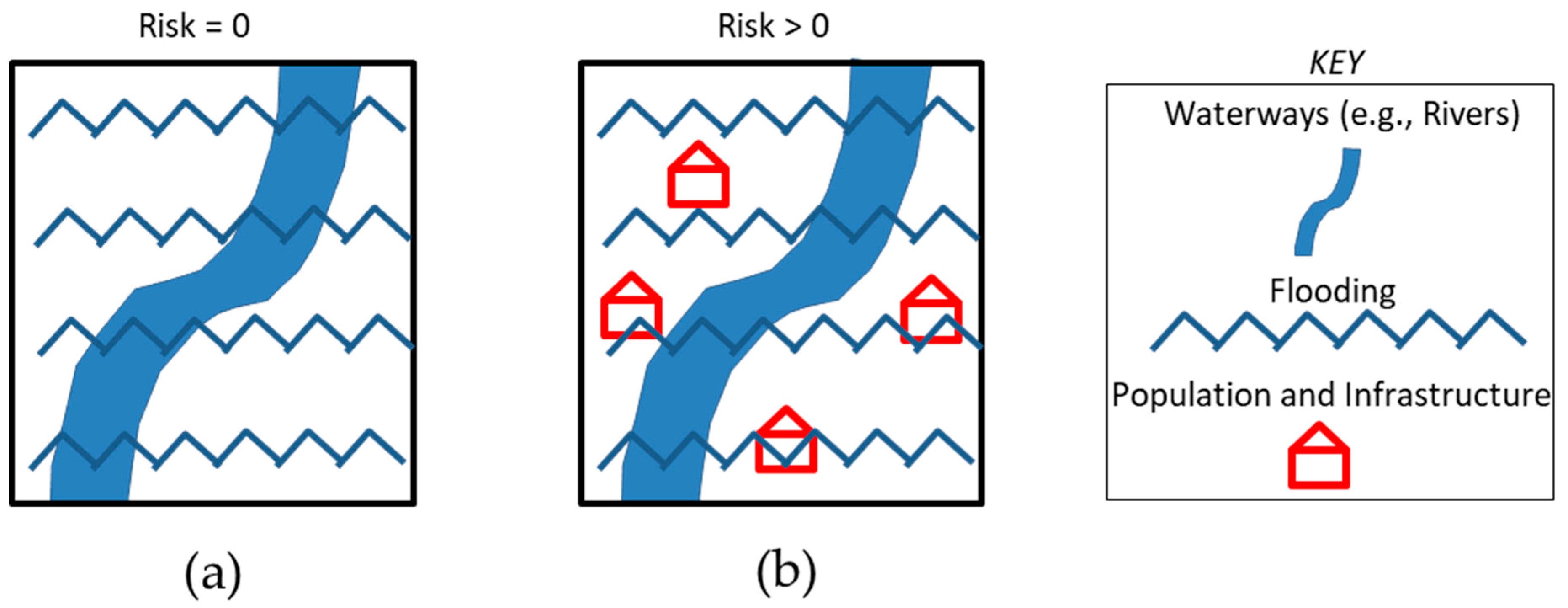
However, flood maps alone are not sufficient to determine and assess the risks to people, property, infrastructure, and services in case of a flood event [3]. Simply put, the impact of the flood is at the minimum if the flooded region is “empty” (unpopulated, has not property, no industry, no infrastructure, and no socio-economic activity) (Figure 1). Therefore, socio-economic factors are critical for risk assessment [4]. Risk assessment is a process or application of a methodology for evaluating risk as defined by the geographic coverage of the hazard, the exposure of people, property, and infrastructure to the hazard, and the vulnerability of people, property, and infrastructure to the event and impact [5]. In previous research on urban flood risk assessments, the majority of studies have focused on the physical systems of urban flood; there are far fewer works on social vulnerability during urban flood disasters [6]. Therefore, it is necessary to develop an approach for the determination of location-based risk indices due to flooding by integrating flood maps, socio-economic parameters, and impacts on infrastructure and services. For a better understanding of the comprehensive impacts of an urban flood disaster, further research is needed to reveal the impact of the uneven distribution of vulnerability, including sensitivity and adaptive capacity, to the disaster in the urban areas.
Due to the need to mitigate flood risk in urban areas, we have selected the Toronto area to demonstrate and test the proposed methodology. Toronto’s population is about 2.5 million, concentrated in an area of 630 km2. The Greater Toronto Area (GTA) covers 7100 km2 with about 5.5 million people. Toronto is socially and geographically a vulnerable city due to its population (largest in Canada, 6th in North America) and its location at the shores of Lake Ontario of the Great Lakes, which is the largest surface water system in the world and where numerous rivers, lakes, and creeks that are part of the large watershed come together. Furthermore, the city is also affected by air masses coming from the Gulf of Mexico, the Atlantic Ocean, and the Arctic. Toronto’s topography is relatively flat, starting at 75 m above sea level at Lake Ontario, to 209 m elevation around the North York area located about a 30 km away from the lake shore. However, the area is characterized by deep ravines, such as the Don River Valley, which is about 400 m wide but only 15 m wide at the river. The City of Toronto and GTA are located in the watersheds of the Don River in the east and the Humber River in the west, both of which drain into Lake Ontario. The Don River watershed is an urban flood-prone area.
2. Related Works
Accurate estimation of flood risk is not a simple issue as multiple factors must be considered. Over the years, various flood risk estimation approaches have been developed in multidisciplinary fields such as GIS, remote sensing, and disaster management.
Using a combination of both fieldwork and a multi-criteria decision analysis algorithm, an approach for flood risk assessment for Vietnam has been developed [7]. Household and field surveys were carried out to gather feedback from local residents to support the definition and selection of flood risk indicators. For hazard indicators, these included a number of categories for various factors such as flood depth (in meters), flood duration (in days), and flood velocity (meters per second). For vulnerability indicators, categories were defined for residential buildings, public institutions (e.g., schools, hospitals, and markets), and agricultural regions. Afterwards, these components were used as input into the decision analysis algorithm known as the Analytical Hierarchy Process (AHP). The AHP was used for the optimal selection of weights for the various indicators. Finally, flood risk was defined as the product of flood hazard and flood vulnerability.
A hybrid GIS and remote sensing-based approach for flood risk determination was produced for Sri Lanka [8]. Datasets included satellite imagery, topographic and GIS data, as well as hydro-meteorological data from rain gauges. This work includes flood simulation analysis using hydrologic (simulates rainfall-runoff in river basins) and hydraulic (used to obtain flood extent and depth) modeling. The simulation was used to verify flood extent regions delineated in the satellite data for hazard determination. The vulnerability was determined using population census data. Again, flood risk was determined to be the product of flood hazard and flood vulnerability.
A flood risk analysis GIS approach using wireless sensor networks has been recently developed [9]. Hydrology-based sensor nodes were deployed on surface water gauges to predict runoff and overflow rates within river basins. Other sensors were used to capture climate-based elements such as humidity levels, air pressure, and wind speed. These parameters were used to determine rainfall intensity.
Probabilistic approaches for flood risk assessment have also been introduced recently, considering flood-related vulnerabilities and fragility relationships. Both are derived from statistical analysis of loss or damage values based on actual observations from past events, simulations, or assumptions of the hazard severity [10]. Researchers have also explored the use of machine learning strategies for flood hazard mapping. Principal component analysis and logistic regression (LR) were used for predicting five flood hazard categories: very low, low, medium, high, and very high [11]. Principal components analysis was used for the selection of the most critical flooding predictor variables. LR is a binary classification model which was used to classify an area as having a flood or no flood. LR was specifically utilized since it provided regression coefficients, which measured the impact of each predictor variable on the flooding classification outcome. A random forest approach, which is a supervised classification scheme, has also been used to model flood risk assessment [12]. Random forests are based on a multitude of decision trees consisting of binary rules. The classification output is computed as the mode of predictions made by each decision tree within the random forest structure. A flood mapping approach based also on random forests was developed where the maps were exclusive of any risk categorization and instead concentrated on identifying and classifying flooded and non-flooded regions using unmanned aerial vehicle imagery [13].
Our approach builds upon the methods for estimating spatial vulnerability, spatial hazard, and spatial risk [14,15], and incorporates the higher spatial resolution and details determined from Earth Observation data. Specifically, the proposed workflow integrates the use of GIS spatial analysis and disaster management principles, which can be visualized in web-mapping browsers for planning and development purposes. This approach can be applied to the development of strategies for future flood risk reduction, risk-based land use planning, resilience, and capacity-building. In particular, it supports spatial decision-making and the development of disaster impact reduction strategies, and the overall effectiveness of disaster management.
3. Methodology
The applied methodology for estimating spatial disaster risk is based on determining risk indices for the selected areal unit. The risk was determined by integrating the values for the flood hazard impact, the vulnerability of people, the exposure of the physical infrastructure (e.g., large building complexes), and the risk resiliency to cope with the flood event. Initially, georeferenced spatial layers were created, representing flood hazard maps, vulnerability maps, and exposure (density of large buildings) maps per areal units.
3.1. Generation of Spatial Data Layers
The vulnerability and susceptibility of the population to damage resulting from the flood hazard is estimated based on socio-economic parameters derived from Statistics Canada Census 2006 data. The Census 2011 data were not used as they do not contain the details of the 2006 Census (e.g., long versus short form for data collection), and the Census 2016 data were not publicly available yet. Social vulnerability is associated with a lack of resources to mitigate, cope with, or recover from disaster. Based on the Statistics Canada Census, social indicators such as age, single-parent families, marital status, education, income, and minority populations were determined. The spatial level Census Tracts (CT) have been used as the areal units for this work. Attribute tables have been generated to link the demographic data as attribute data to these areal units.
The exposure spatial layers may contain the physical components of the urban system, such as infrastructure elements. These could be buildings (residential, commercial, industrial) and critical facilities (road and rail networks, healthcare facilities, educational institutions, ambulance, fire and police stations, airports, land cover/use). These elements can be acquired from various spatial databases and EO. A process can be developed to assign a level of significance for their location. For this project, the density of large building complexes per CT was used to demonstrate the exposure hazard.
The flood hazard spatial layer consists of areas that are susceptible to flooding, such as water bodies (e.g., floodplain maps), areas of low slope, land depressions, and certain areas of land cover element (e.g., bare soil, impervious surfaces). These have been obtained from the land cover map provided by the Canada Center for Mapping and Earth Observation (CCMEO) based on WorldView-2 satellite imagery. These terrain features, such as flood line boundaries (provided by the Toronto and Region Conservation Authority (TRCA)), land depressions, and areas of low terrain slope are used to assign different spatial impact weights (e.g., areas of water concentration and areas of high/low water depth).
3.2. Estimation of Spatial Flood Risk Index
The spatial risk index for each spatial areal unit (Census Tract) within each flood hazard zone has been estimated using a spatial layer overlay operation between the hazard and the spatial layers of flood consequences. The consequences layers were generated based on the spatial intersection of the vulnerability and exposure layers. Spatial intersection is performed using a raster multiplication operation. An index value for each grid raster cell is estimated and a ranked map based on the index values has been generated.
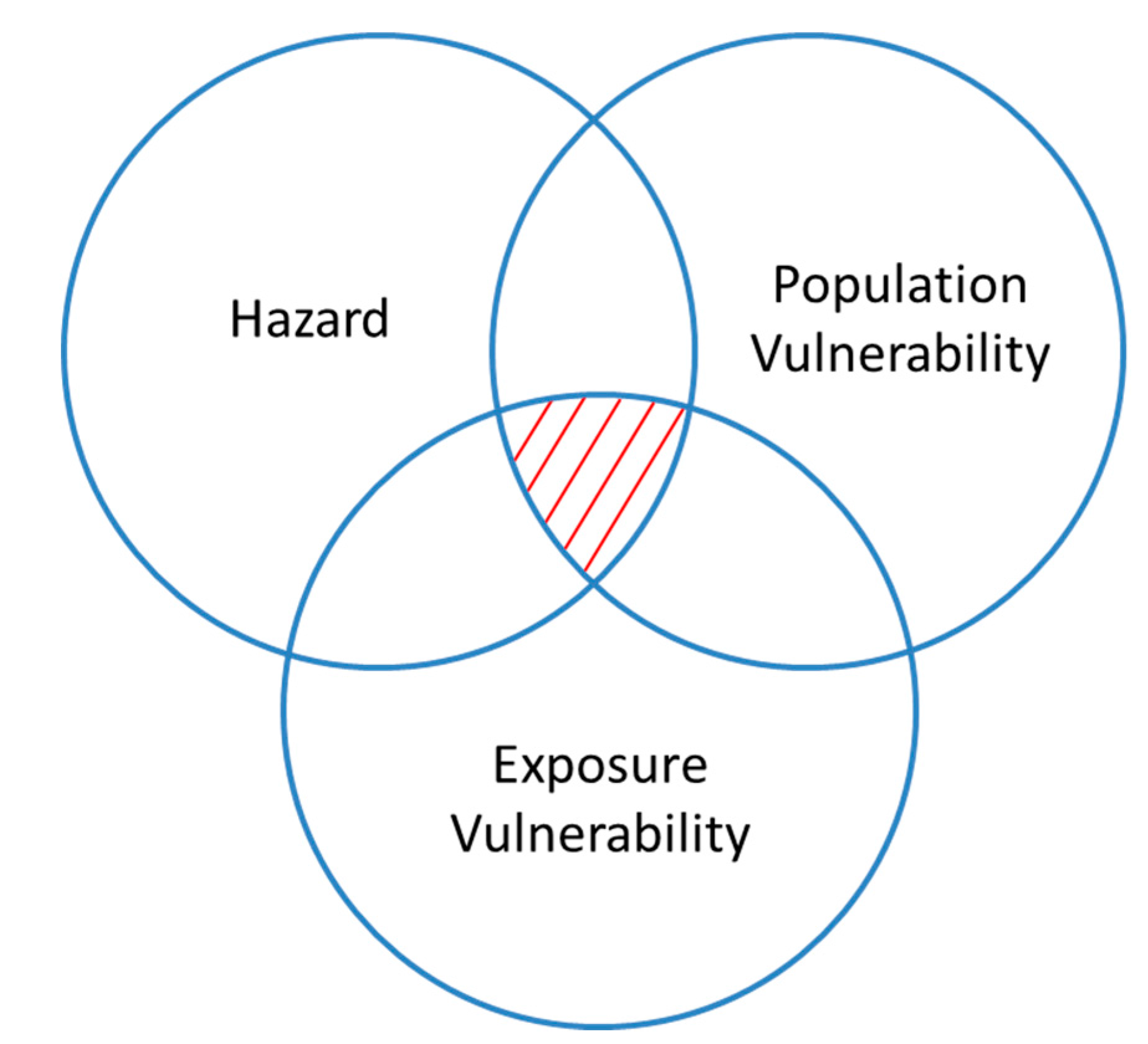
Therefore, the flood risk (RF) map, as defined by Equation (1), is the spatial intersection of flood hazard, social (population) and exposure vulnerability (Figure 2), and resilience spatial layers.
where,
- HF: is the flood hazard spatial layer and is equal to , where is the various flood hazards related to the areal components;
- VP: is the social vulnerability spatial layer and is equal to , where is the various population vulnerabilities related to the areal components;
- VE: is the exposure of infrastructure vulnerability spatial layer and is equal to , where is the various infrastructure related to the areal components;
- G: is the Resilience, expressing the degree of the ability to adapt and recover from the disaster.
It values range from 0 to 1, where 0 is very high resilience (no risk) and 1 is no resilience (no reduction of the risk).
Various weights can be used based on the expected impact of each contributing component to the estimated risk.
4. Study Area and Data
The study area is the common area between the Don River watershed (in blue) and the administrative boundary of the Greater Toronto Area (GTA) (in red), shown with the green dashed lines (Figure 3). The city of Toronto has experienced many major floods over the past century: the flood following hurricane Hazel on 15 October 1954, the 27 August 1976 floods, and the floods on 19 August 2005, 8 July 2013, 25 June 2014, 23 June 2015, and 27 July and 17 August 2016. For example, during the 8 July 2013 flooding, some parts of the City of Toronto received over 120 mm of rain, while the monthly average for Toronto is 74.4 mm. The impact was felt as 300,000 residents were affected by power outages. Other serious disruptions included flight cancellations and subway and other transportation closures. It was the most expensive disaster for the province of Ontario. According to the Insurance Bureau of Canada, the damage to the insured properties exceeded $850 million [16].
Location-based estimation of flood risk in urban areas supports flood disaster management operations and particularly those of mitigation and response. Essentially, the estimated risk is managed by taking measures to reduce the exposure and vulnerability of identified urban elements to the flood hazard [5].
The following data have been used.
Raw Data
- GTA Administrative boundary.
- Don River watershed.
- Flood lines polygon representation of the TRCA’s feature classes “Engineered Flood line” and “Estimated Flood line”. The “Estimated Flood line” used in this work has been altered from the original estimated flood plain as it has been clipped to where the “Engineered Flood line” has superseded it.
- Land Cover, classified data derived by WorldView-2 satellite imagery, ground pixel size 2 m × 2 m.
- Digital Elevation Model (DEM)—Provincial Tiled Dataset, ground pixel size 10 m × 10 m, with 32 bit pixel depth.
- Census tract boundaries, vector polygonal data, Statistics Canada.
- Demographics data—Tabular data, Census 2006, Statistics Canada.
- Toronto building footprints, vector polygonal data generated using Enterprise Stereoscopic Model (ESM) digital topographic map data and Property Data Map (PDM) data from the City of Toronto Geospatial Competency Centre (GCC), based on an in-house built data model. The original data is as of 2005, and it is updated against 2015 aerial photographs and Toronto building permit drawings. The polygon file contains the average height of buildings from Mean Sea Level and Building height for buildings in the entire city. The data is used for 3D context massing illustration and visualization purposes only.
- A point feature layer for large buildings shows the locations of buildings. Each point represents the centroid of a building footprint. Some features include additional data pertaining to address, building type, and building name.Note: Some of the Census Track data was missing as noted in the outcome maps.
Derived data from the DEM
- Slope
- Land Depression
All the data used were either already in, or converted to, raster format with a ground resolution of 10 m × 10 m. This was based on the resolution of the DEM data. Spatial Reference: NAD 1983 UTM Zone 17N.
5. Implementation and Results
5.1. Determination of Vulnerability
Two vulnerability spatial layers were derived based on the CT areas: the social population vulnerability based on the Census 2016 population data, and the exposure vulnerability based on the density of large building structures within each CT.
Social vulnerability comprises socio-economic and demographic indicators, such as age, gender, education level, and income level, which are affected by floods [17,18,19]. Social vulnerability is associated with a lack of resources to mitigate, cope with, or recover from disaster. Social vulnerability is clearly visible as the result of the impact of a disaster. Groups of people that are especially at risk are clearly defined in [20,21]. The 2006 Census Tracts data from Statistics Canada has been used to extract demographic information on vulnerable groups. We followed the approach given in [15]. The ten demographic category attributes used to determine social vulnerability are:
- -
- People 65 years and older
- -
- Children 4 years and younger
- -
- Single parents with young children
- -
- Households with children under 6 years old
- -
- Rented apartments
- -
- Non-English- or French-speaking people
- -
- Unemployed
- -
- Unpaid for work
- -
- High school education or less
- -
- Family income of less than $50,000 after tax.
In order to standardize various data types for each category, percentage values for each of the ten categories were calculated based on total population in the corresponding census tract (CT). The total normalized weighted vulnerability for each CT is calculated as:
where,
- VPCT: total vulnerability per each CT
- Ci: category attribute
- %Ci: category attribute percentage with respect to population in the CT
- P: total CT population.
Exposure vulnerability relates to man-made infrastructure elements which are affected by flooding. In this case, VE for each CT was defined as the normalized density of large buildings per census tract area:
where,
- VECT: exposure vulnerability for each CT area
- BCT: number of large building complexes within the CT
- ACT: area of the CT
- i: number of CTs.
The total vulnerability was determined as the spatial intersection between the two vulnerabilities (Figure 4).
5.2. Determination of Flood Hazard Areas
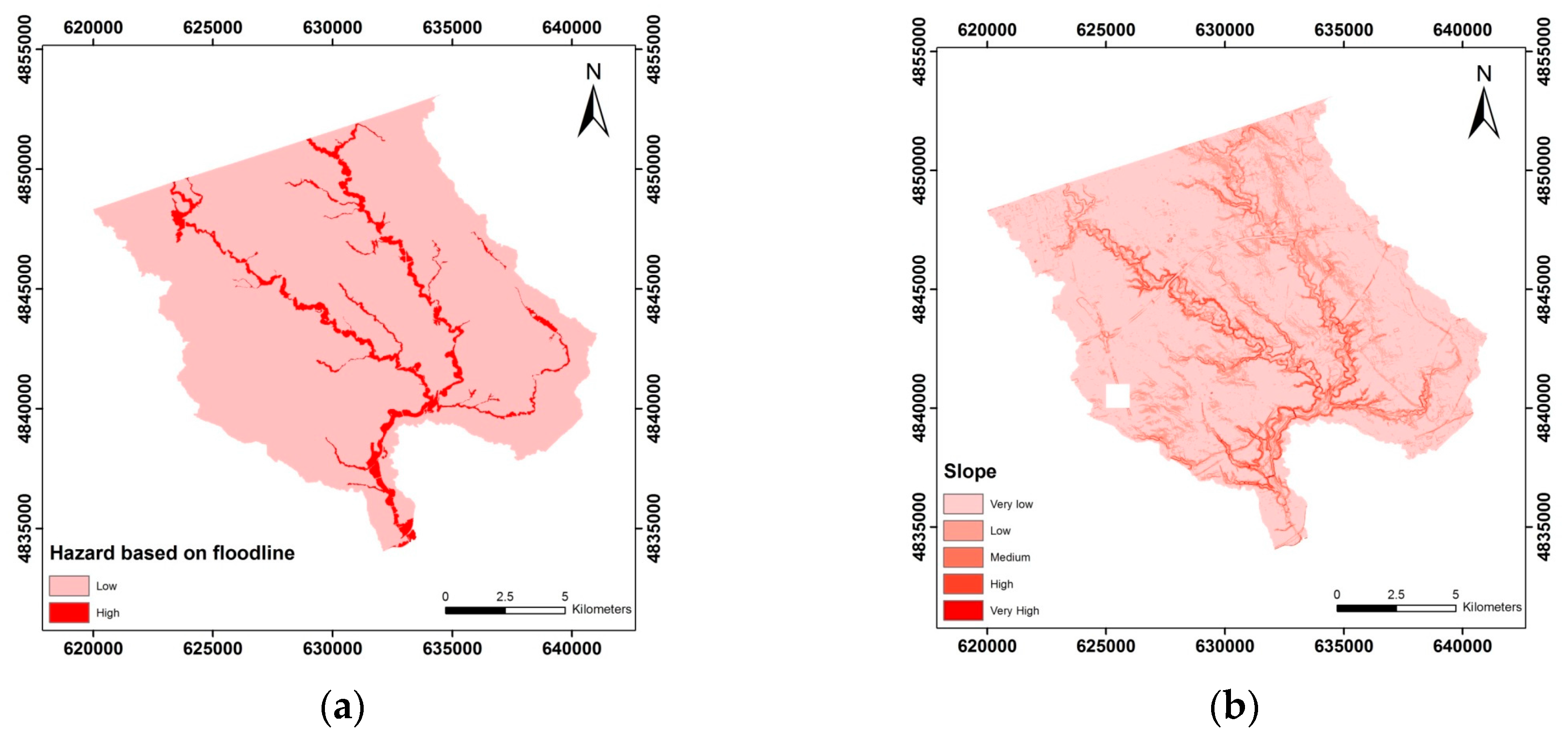
The flood hazard spatial layer consists of areas that are susceptible to flooding, such as water bodies (e.g., floodplain maps), areas of low slope, land depressions, and certain elements of land cover (e.g., bare soil, impervious surfaces). The flood hazard areas were determined as the weighted average of the following elements, which contribute to a flood event (Equation (4)). These are:
- -
- the flood lines (provided by TRCA) delineating the flood plains around the rivers in the study area (Figure 5a),
- -
- the areas of slope of less than 2% derived from the DEM data (Figure 5b),
- -
- the areas of land depressions generated as the fill DEM minus the actual DEM localizing the sink type areas in the region (Figure 5c), and
- -
- the land cover areas of vegetation, water, impervious surfaces, bare soil and grasslands (Figure 5d).
- HF: is the total hazard
- HFi: are the individual hazards
- wi: are the weights empirically set based on the significance ranking of each hazard area (w1 = 0.4 for flood lines, w2 = 0.1 for land depressions, w3 = 0.25 for slope of less than 2% and w4 = 0.25 for land cover).
The total flood hazard map derived by Equation (4) is shown in Figure 6.
5.3. Generation of Flood Risk Maps
The following three flood risk maps have generated based on the total flood hazards:
- (i).
- Flood risk map (A) based on Total Flood Hazard and Total Social vulnerability derived using Equation (5) and shown in Figure 7,
- (ii).
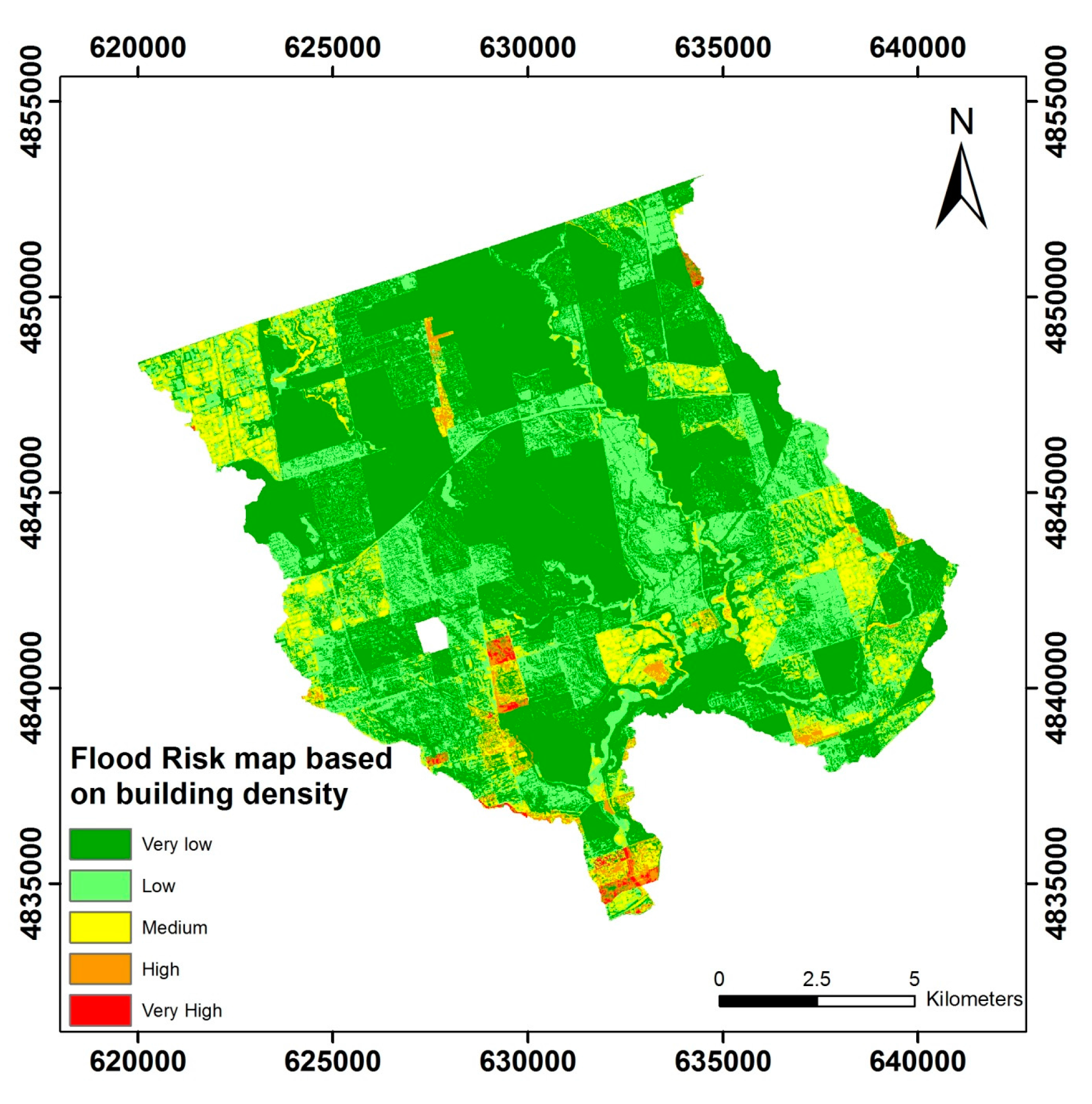
- Flood risk map (B) based on Total Flood Hazard and Total Exposure vulnerability derived using Equation (6) and shown in Figure 8,
- (iii).
- Flood risk map (C) based on Total Flood Hazard and Total vulnerability (Social and Exposure) using Equation (7) and shown in Figure 9:with weights wP = 0.7, wE = 0.3, respectively, and set empirically based on the significance impact of each vulnerability component.
6. Results Discussion and Concluding Remarks
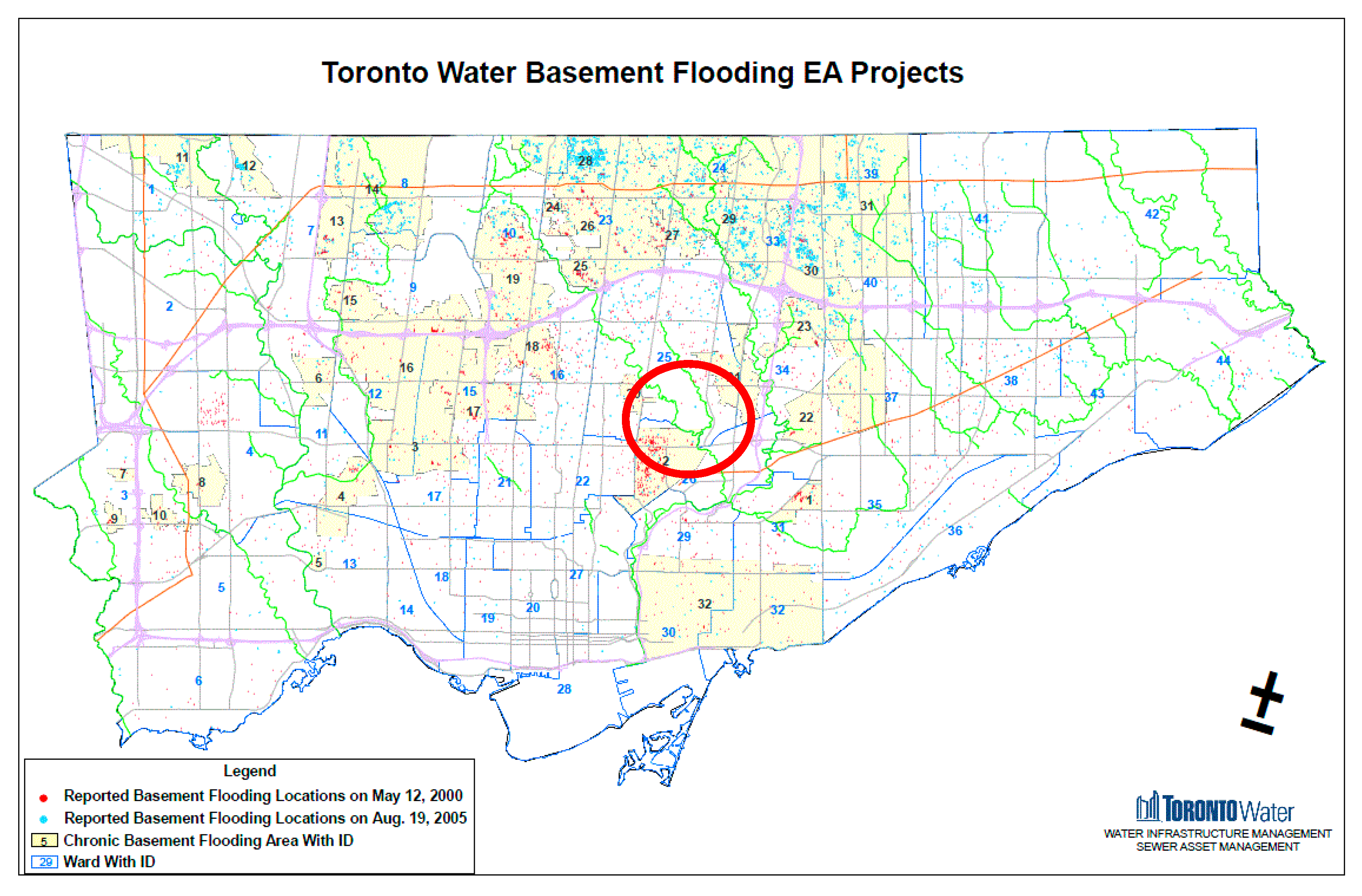
Preliminary validation of the results based on existing published flooding maps (Figure 10 and Figure 11) indicate an apparent agreement in flooding locations (circular-marked regions) with the red circled area in Figure 9.
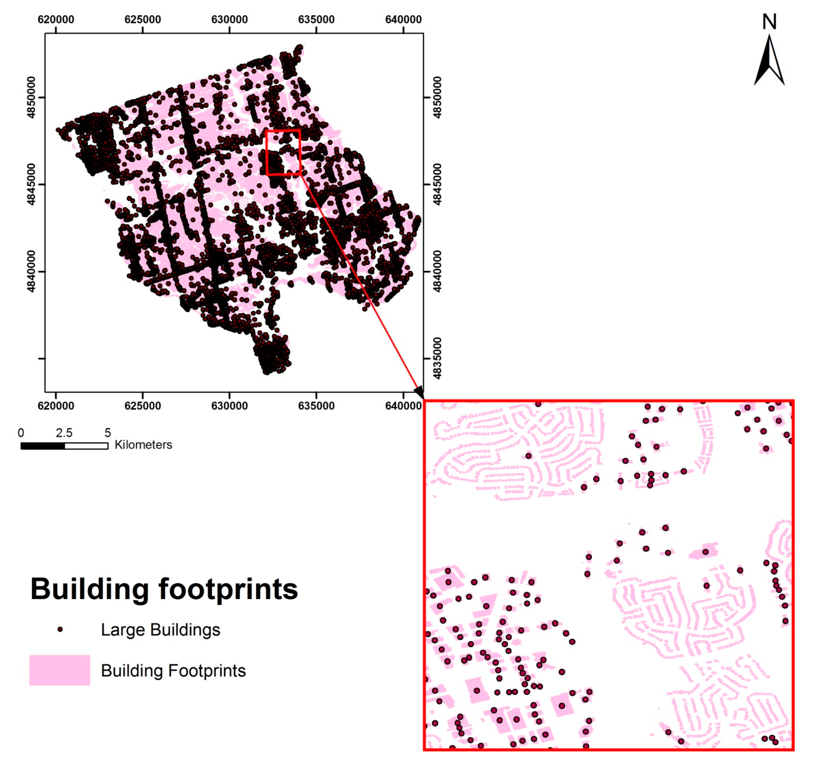
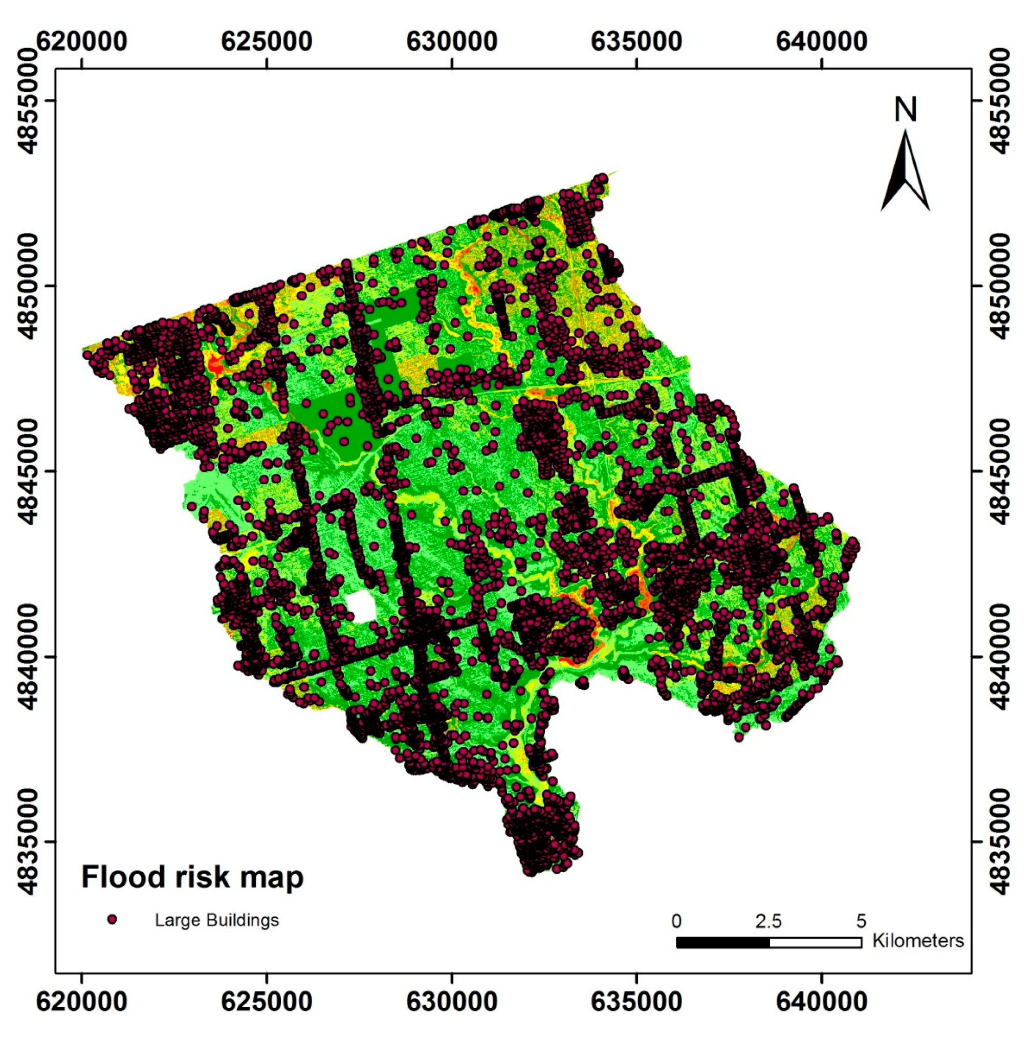
Visual inspection of the final risk maps indicate that the areas of higher flood risk coincide with (a) areas of high flood hazard (e.g., flood line); (b) areas of high social vulnerability; and (c) areas of high exposure vulnerability expressed as high density of large building structures (Figure 12 and Figure 13).
The knowledge of flood risk supports the disaster risk management cycle, which includes prevention, preparedness, response, and rehabilitation. In this work, the flood risk has been determined not only considering the physical process of flooding (water-level rise, water inundation) but also considering the impact of a flood event on population and infrastructure elements. For this process, spatial modeling has been applied for flood risk estimation based on the spatial intersection of the hazard and vulnerability raster layers. Various additional spatial layers can be also added and used to perform sensitivity analysis. Based on the preliminary results, we have observed consistency with a limited sample of ‘reference’ data indicating known flood-prone areas. Further validation is required, in collaboration with the relevant flooding management authorities for Toronto (such as the TRCA). The methodology is capable of providing total flood risk maps, as well as flood risk maps related to specific vulnerable classes (i.e., social vs. infrastructure). The weights used for the contribution of hazard and vulnerability elements were set by the project team without consulting subject matter experts due to the limited time constraints of the project. Methods such as multi-criteria analysis can be used in the future for the determination of the contribution weights. The use of data from the rain and flood gauges should also be considered. Further, different mathematical models can also be investigated to improve the flood risk estimation.
Acknowledgments
This work has been funded by Canada Center for Mapping and Earth Observation (CCMEO), Natural Resources Canada (NRCan). We are thankful to Rosa Orlandini, Head, Map Library/Librarian, York University, for her advice and guidance in finding the various data sets used in this project. We also very thankful to Dan Clayton, Senior Project Manager, Information Management Group, Toronto and Region Conservation Authority (TRCA) and the TRCA for providing the flood line data in the Don River watershed.
Author Contributions
Costas Armenakis and Ravi Ancil Persad conceived and designed the experiments; Erin Xinheng Du and Sowmya Natesan performed the experiments; Costas Armenakis, Erin Xinheng Du, Sowmya Natesan, Ravi Ancil Persad and Ying Zhang analyzed the data; Ying Zhang contributed data; Costas Armenakis drafted the paper and all authors contributed to its final version.
Conflicts of Interest
The authors declare no conflict of interest.
References
- Altan, O.; Backhaus, R.; Boccardo, P.; Zlatanova, S. Geoinformation for Disaster and Risk Management; Joint Board of Geospatial Information Societies: Copenhagen, Denmark, 2010. [Google Scholar]
- Safaripour, M.; Monavari, M.; Zare, M.; Abedi, Z.; Gharagozlou, A. Floor risk assessment using GIS (Case study: Golestan Province, Iran). Pol. J. Environ. Stud. 2012, 21, 1817–1824. [Google Scholar]
- Federal Emergency Management Agency (FEMA). Guidance for Flood Risk Analysis and Mapping—Flood Risk Assessments; Federal Emergency Management Agency (FEMA): Washington, DC, USA, 2014.
- National Research Council; Committee on Population. Tools and Methods for Estimating Populations at Risk from Natural Disasters and Complex Humanitarian Crises; National Academies Press: Washington, DC, USA, 2007. [Google Scholar]
- UN Office for Disaster Risk Reduction (UNISDR). Component of Risk—Disaster Risk, Global Assessment Report; Prevention Web, Serving the Information Needs of the Disaster Reduction Community; UNISDR: Geneva, Switzerland, 2015. [Google Scholar]
- Cho, S.Y.; Chang, H. Recent research approaches to urban flood vulnerability, 2006–2016. Nat. Hazards 2017, 88, 633–649. [Google Scholar] [CrossRef]
- Dang, N.M.; Babel, M.S.; Luong, H.T. Evaluation of food risk parameters in the day river flood diversion area, Red River delta, Vietnam. Nat. Hazards 2011, 56, 169–194. [Google Scholar] [CrossRef]
- Samarasinghea, S.M.J.S.; Nandalalb, H.K.; Weliwitiyac, D.P.; Fowzed, J.S.M.; Hazarikad, M.K.; Samarakoond, L. Application of remote sensing and GIS for flood risk analysis: A case study at Kalu-Ganga river, Sri Lanka. Int. Arch. Photogramm. Remote Sens. Spat. Inf. Sci. 2010, 38, 110–115. [Google Scholar]
- Ahmad, N.; Hussain, M.; Riaz, N.; Subhani, F.; Haider, S.; Alamgir, K.S.; Shinwari, F. Flood prediction and disaster risk analysis using GIS based wireless sensor networks, a review. J. Basic Appl. Sci. Res. 2013, 3, 632–643. [Google Scholar]
- Pregnolato, M.; Galasso, C.; Parisi, F. A Compendium of Existing Vulnerability and Fragility Relationships for Flood: Preliminary Results. In Proceedings of the 12th International Conference on Applications of Statistics and Probability in Civil Engineering, ICASP12, Vancouver, BC, Canada, 12–15 July 2015. [Google Scholar]
- Nandi, A.; Mandal, A.; Wilson, M.; Smith, D. Flood hazard mapping in Jamaica using principal component analysis and logistic regression. Environ. Earth Sci. 2016, 75, 465. [Google Scholar] [CrossRef]
- Wang, Z.; Lai, C.; Chen, X.; Yang, B.; Zhao, S.; Bai, X. Flood hazard risk assessment model based on random forest. J. Hydrol. 2015, 527, 1130–1141. [Google Scholar] [CrossRef]
- Feng, Q.; Gong, J.; Liu, J.; Li, Y. Flood mapping based on multiple endmember spectral mixture analysis and random forest classifier—The case of Yuyao, China. Remote Sens. 2015, 7, 12539–12562. [Google Scholar] [CrossRef]
- Armenakis, C.; Nirupama, N. Estimating spatial disaster risk in urban environments. Geomat. Nat. Hazards Risk 2013, 4, 289–298. [Google Scholar] [CrossRef]
- Armenakis, C.; Nirupama, N. Flood risk mapping for the city of Toronto. Procedia Econ. Financ. 2014, 18, 320–326. [Google Scholar] [CrossRef]
- Toronto Star. Toronto’s July Flood Listed as Ontario’s Most Costly Natural Disaster, by Carys Mills, Published on Wednesday, 14 August 2013. Available online: http://www.thestar.com/business/2013/08/14/july_flood_ontarios_most_costly_natural_disaster.html (accessed on 22 November 2017).
- Weichselgartner, J. Disaster mitigation: The concept of vulnerability revisited. Disaster Prev. Manag. 2001, 10, 85–94. [Google Scholar] [CrossRef]
- Adelekan, O.I. Vulnerability assessment of an urban flood in Nigeria: Abeokuta flood 2007. Nat. Hazards 2011, 56, 215–231. [Google Scholar] [CrossRef]
- Opolot, E. Application of remote sensing and geographical information systems in flood management: A review. Res. J. Appl. Sci. Eng. Technol. 2014, 6, 1884–1894. [Google Scholar]
- Ferrier, N.; Haque, E. Hazards risk assessment methodology for emergency managers: A standardized framework for application. Nat. Hazards 2003, 28, 271–290. [Google Scholar] [CrossRef]
- Provincial Emergency Preparedness (PEP). Hazard, Risk, and Vulnerability Analysis Toolkit; Provincial Emergency Preparedness Publication: Vancouver, BC, Canada, 2004; p. 66. [Google Scholar]
Figure 1.
Understanding flooding risk. (a) Flooded area is “empty”, thus flood risk is zero; (b) Flooded are contains population and infrastructure, thus flood risk is greater than zero.
Figure 1.
Understanding flooding risk. (a) Flooded area is “empty”, thus flood risk is zero; (b) Flooded are contains population and infrastructure, thus flood risk is greater than zero.

Figure 2.
Schematic diagram of risk definition (red area).

Figure 3.
Study area (dashed green lines). The blue region is the Don River watershed, with an extent of 38 km emptying into Lake Ontario, Canada. The red vector layer represents the Greater Toronto Area, which is a heavily populated conurbation.
Figure 3.
Study area (dashed green lines). The blue region is the Don River watershed, with an extent of 38 km emptying into Lake Ontario, Canada. The red vector layer represents the Greater Toronto Area, which is a heavily populated conurbation.
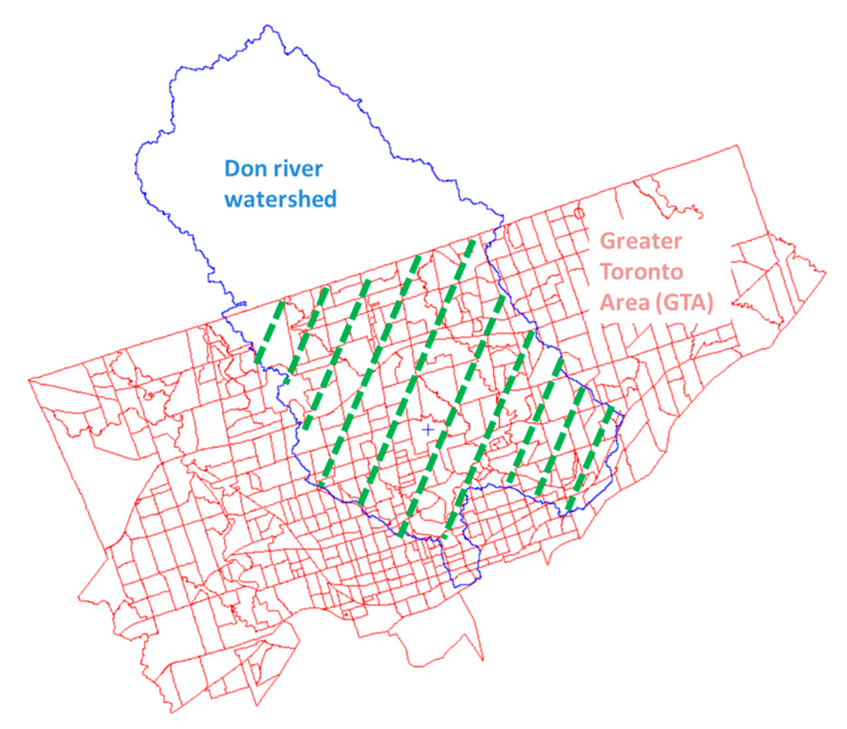
Figure 4.
Vulnerability maps. (a) Social vulnerability map (low green Census Tracts (CT) reflects missing Census data); (b) Exposure vulnerability map; (c) Total flood vulnerability map.
Figure 4.
Vulnerability maps. (a) Social vulnerability map (low green Census Tracts (CT) reflects missing Census data); (b) Exposure vulnerability map; (c) Total flood vulnerability map.
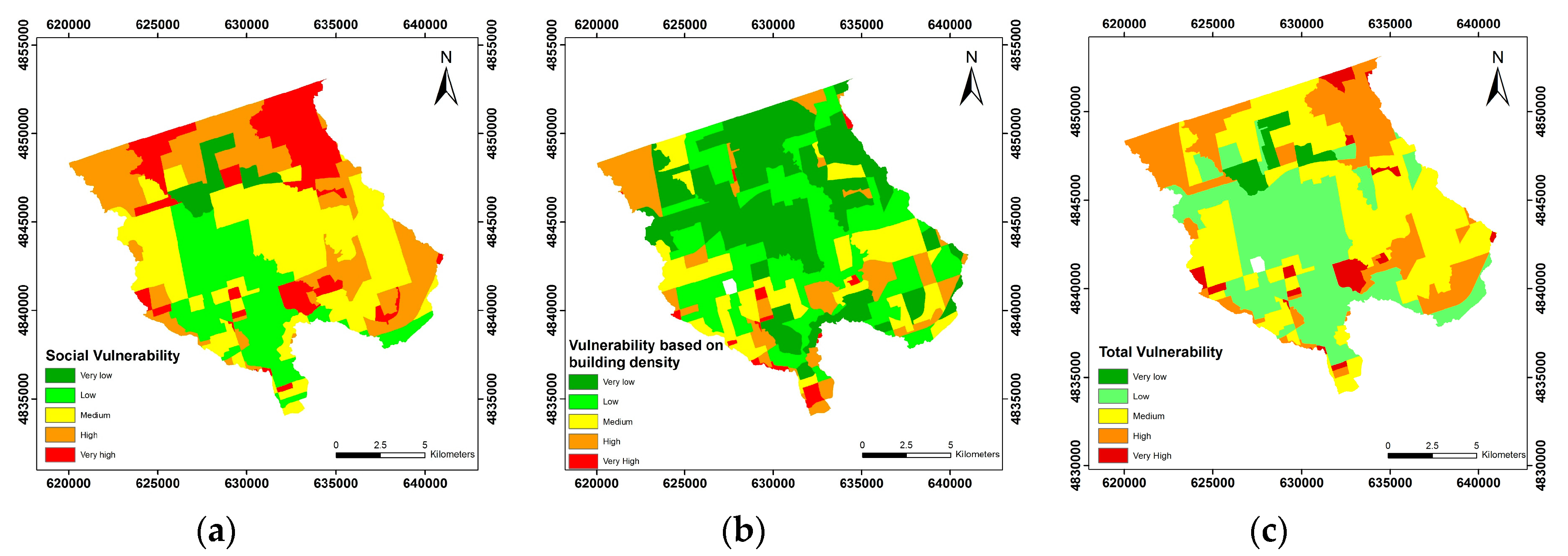
Figure 5.
Flood hazard areas maps. (a) Based on Don River flood lines; (b) based on terrain slope; (c) based on land depressions; (d) based on land cover areas of vegetation, water, impervious surfaces, bare soil, and grasslands.
Figure 5.
Flood hazard areas maps. (a) Based on Don River flood lines; (b) based on terrain slope; (c) based on land depressions; (d) based on land cover areas of vegetation, water, impervious surfaces, bare soil, and grasslands.


Figure 6.
Total flood hazard map.
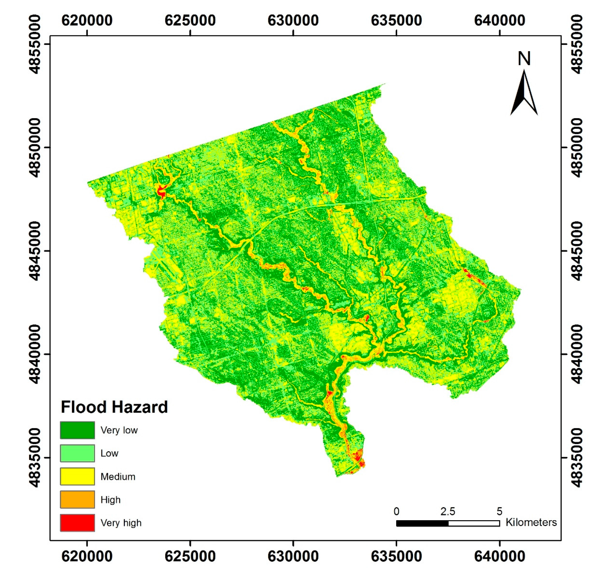
Figure 7.
Flood risk map based on total flood hazard and total social vulnerability. Note: In the upper region of the map, there are three distinct (green) polygon regions characterized with very low risk due to lack of data.
Figure 7.
Flood risk map based on total flood hazard and total social vulnerability. Note: In the upper region of the map, there are three distinct (green) polygon regions characterized with very low risk due to lack of data.

Figure 8.
Flood Risk map based on total hazard and total exposure vulnerability.
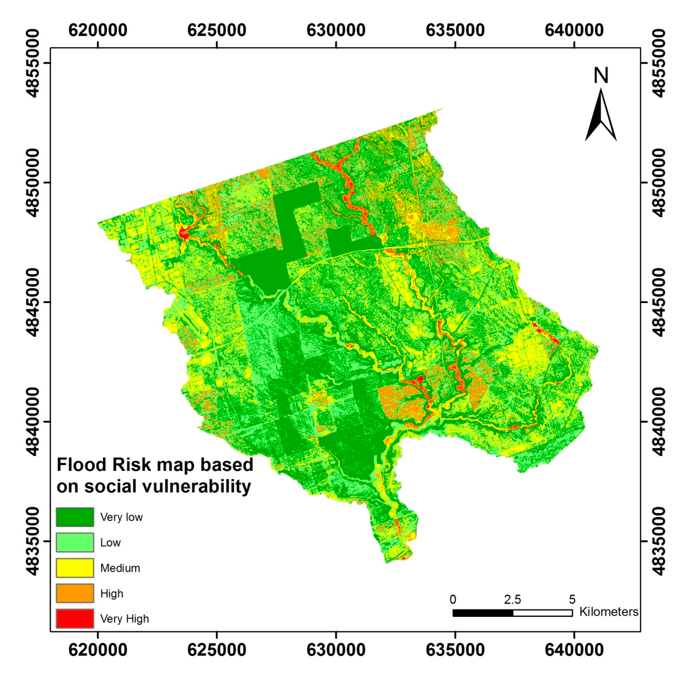
Figure 9.
Flood Risk map based on total flood hazard and total vulnerability. Note: In the upper region of the map, there are three distinct (green) polygon regions characterized with very low risk due to lack of data. The circular red marker indicates a validation area.
Figure 9.
Flood Risk map based on total flood hazard and total vulnerability. Note: In the upper region of the map, there are three distinct (green) polygon regions characterized with very low risk due to lack of data. The circular red marker indicates a validation area.

Figure 10.
Water basement flooding in Greater Toronto Area in 2000 and 2005. Source: http://www.cityfloodmap.com/2014/07/toronto-flood-map.html.
Figure 10.
Water basement flooding in Greater Toronto Area in 2000 and 2005. Source: http://www.cityfloodmap.com/2014/07/toronto-flood-map.html.

Figure 11.
Reported Flooding Locations (Example looking northeast from Toronto Harbour). Blue markers: 12 May 2000 storm; Pink markers: 19 August 2005 storm. Source: http://www.cityfloodmap.com/2014/07/toronto-flood-map.html.
Figure 11.
Reported Flooding Locations (Example looking northeast from Toronto Harbour). Blue markers: 12 May 2000 storm; Pink markers: 19 August 2005 storm. Source: http://www.cityfloodmap.com/2014/07/toronto-flood-map.html.
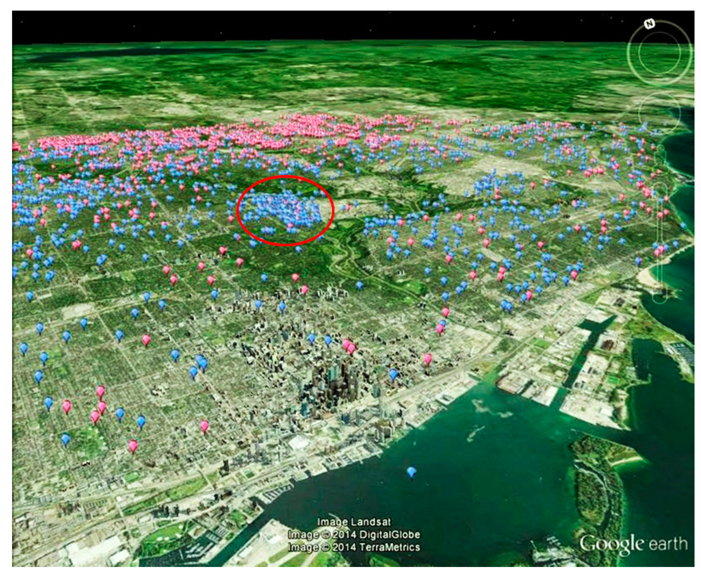
Figure 12.
Building footprints and points of large buildings.

Figure 13.
Large buildings superimposed on the Flood Risk map.
© 2017 by the authors. Licensee MDPI, Basel, Switzerland. This article is an open access article distributed under the terms and conditions of the Creative Commons Attribution (CC BY) license (http://creativecommons.org/licenses/by/4.0/).
Share and Cite
MDPI and ACS Style
Armenakis, C.; Du, E.X.; Natesan, S.; Persad, R.A.; Zhang, Y. Flood Risk Assessment in Urban Areas Based on Spatial Analytics and Social Factors. Geosciences 2017, 7, 123. https://doi.org/10.3390/geosciences7040123
AMA Style
Armenakis C, Du EX, Natesan S, Persad RA, Zhang Y. Flood Risk Assessment in Urban Areas Based on Spatial Analytics and Social Factors. Geosciences. 2017; 7(4):123. https://doi.org/10.3390/geosciences7040123
Chicago/Turabian StyleArmenakis, Costas, Erin Xinheng Du, Sowmya Natesan, Ravi Ancil Persad, and Ying Zhang. 2017. "Flood Risk Assessment in Urban Areas Based on Spatial Analytics and Social Factors" Geosciences 7, no. 4: 123. https://doi.org/10.3390/geosciences7040123
Note that from the first issue of 2016, this journal uses article numbers instead of page numbers. See further details here.