Supercontinent Cycle and Thermochemical Structure in the Mantle: Inference from Two-Dimensional Numerical Simulations of Mantle Convection


Geodynamics Research Center, Ehime University, 2–5 Bunkyo-cho, Matsuyama 790-8577, Ehime, Japan
*
Author to whom correspondence should be addressed.
Geosciences 2017, 7(4), 126; https://doi.org/10.3390/geosciences7040126
Submission received: 27 September 2017
/
Revised: 13 November 2017
/
Accepted: 30 November 2017
/
Published: 5 December 2017
(This article belongs to the Special Issue Mantle Circulation and Plate Movement)
Abstract
:In this study, we conduct numerical simulations of thermochemical mantle convection in a 2D spherical annulus with a highly viscous lid drifting along the top surface, in order to investigate the interrelation between the motion of the surface (super)continent and the behavior of chemical heterogeneities imposed in the lowermost mantle. Our calculations show that assembly and dispersal of supercontinents occur in a cyclic manner when a sufficient amount of chemically-distinct dense material resides in the base of the mantle against the convective mixing. The motion of surface continents is significantly driven by strong ascending plumes originating around the dense materials in the lowermost mantle. The hot dense materials horizontally move in response to the motion of continents at the top surface, which in turn horizontally move the ascending plumes leading to the breakup of newly-formed supercontinents. We also found that the motion of dense materials in the base of the mantle is driven toward the region beneath a newly-formed supercontinent largely by the horizontal flow induced by cold descending flows from the top surface occurring away from the (super)continent. Our findings imply that the dynamic behavior of cold descending plumes is the key to the understanding of the relationship between the supercontinent cycle on the Earth’s surface and the thermochemical structures in the lowermost mantle, through modulating not only the positions of chemically-dense materials, but also the occurrence of ascending plumes around them.
1. Introduction
It is often conjectured that the assembly and dispersal of supercontinents occurred several times during the Earth’s history (e.g., [1]). This cyclic behavior, commonly termed “supercontinent cycle” or “Wilson cycle” [2], includes the formation of Pangea (about 330 Ma) and its breakup (starting about 175 Ma) [3,4,5], the formation of Rodinia (about 900 Ma) and its breakup (during 825 and 750 Ma) [6] and those of far earlier ones. Among the events of breakup, some are caused by the impingement of ascending plumes beneath the supercontinent [7], even though some do not have any sign of ascending plumes [8]. This fact suggests the significance of the interrelations between the supercontinents and ascending plumes from the deep mantle in driving the supercontinent cycle. In particular, it is of crucial importance to understand the mechanism that generates ascending plumes in a cyclic manner in response to the assembly and dispersal of supercontinents.
On the other hand, it has been also well acknowledged that the generation of ascending plumes from the deep mantle is significantly affected by the presence of chemical heterogeneities in the mantle (e.g., [9]). One of the most relevant examples is the large low-shear velocity provinces (LLSVPs) in the lowermost mantle beneath the Pacific Ocean and Africa (for a review, see [10]). From several lines of seismological evidence, such as their sharp-sided structure, low V/V ratio and increased density, it is generally considered that the LLSVPs are chemically distinct from the surrounding, although some recent studies suggest their thermal origin [1,11,12]. Moreover, Burke and coworkers demonstrated the spatial correlations between the eruption sites of large igneous provinces (LIPs) [13] within recent 300 Ma and the distributions of S-wave perturbation in the lowermost mantle [14,15,16]: the hot ascending plumes originate from the margins of the LLSVPs, not from elsewhere or not from within the LLSVPs. These observations suggest that the presence of chemical heterogeneity in the lowermost mantle restricts the regions of origin of ascending plumes at least for the latest 300 Ma, although it is still controversial how strongly a chemical heterogeneity tends to fix the roots of ascending plumes [17]. This further implies an interrelation between the supercontinent cycle at the Earth’s surface and the distributions of chemical heterogeneity in the lowermost mantle, through the generation of ascending plumes.
In this study, we will conduct numerical experiments of thermochemical mantle convection, which incorporates the effects of the presence and drifting motion of the surface continent. The aim of this study is to investigate the interrelation between the motion of the surface (super)continent and the behavior of chemical heterogeneities in the lowermost mantle, both of which are thought to be related to the ascending plumes in the mantle. As can be inferred from the interrelations with the generation of ascending plumes, the operation of the supercontinent cycle at the Earth’s surface is aided by a cyclic change in the lateral distributions of chemical heterogeneity in the deep mantle. We will in particular focus on the conditions under which the supercontinent cycle, i.e., the cyclic assembly and dispersal, can take place in concert with the presence of chemical heterogeneity in the lowermost mantle. As will be described later, our study relies on an extremely simplified numerical model of thermochemical convection in the mantle and drifting motion of the continental lid along the top surface. Despite the simplicity, we do believe that our model captures the fundamental nature of the interrelation between the motion of the surface (super)continent and the behavior of chemical heterogeneities in the lowermost mantle.
2. Model Description
We consider a time-dependent basally-heated convection of a two-component fluid in a model of a two-dimensional spherical annulus spanning an angle of radians (180) whose outer and inner radii are and , respectively. The values of and are taken to satisfy and km, in order to mimic the values of the Earth’s mantle. Both the top () and bottom () surfaces are taken to be impermeable (i.e., zero normal velocity) and free-slip (i.e., zero traction). On the other hand, we assumed mirror symmetry at the vertical side walls ( and ), in order to reproduce convection cells with the largest horizontal wavelength. This allows us to virtually consider the convection in a full spherical annulus spanning an angle of radians (360) with low computational costs.
Temperature is fixed to be (= 0 C) and (= 3500 C) at the top and bottom boundaries, respectively. We take into account the effect of the endothermic phase transition between ringwoodite and bridgmanite plus ferropericlase at around a 660-km depth from the top surface. In addition, we impose a lid of highly viscous fluid along the top surface (e.g., [18,19,20]) as a model of the (super)continent, whose vertical and horizontal dimensions are fixed to be km and radians, respectively. That is, the continental lid is taken to occupy a third of the top surface (). We also take into account the assembly and breakup of a supercontinent, by allowing a coherent horizontal motion of continental lid driven by the overall convection in the mantle. In this study, we mean by the presence of a “supercontinent” the state where the continental lid is in contact with vertical side walls: owing to the mirror symmetry at or , the lid is combined with its mirror image to form a supercontinent whose horizontal dimension is .
Before going into the detailed description of our numerical model, we admit that intensive simplifications were made in developing our model. For example, we assumed that thermal convection in the mantle takes place solely by the heating from the bottom and, in other words, ignored the effect of internal heating. This means that our model is unable to correctly reproduce not only the thermal evolution of the mantle owing to the lack of dominant heat sources, but also the styles of mantle convection such as horizontal wavelength (e.g., [21,22]), the relative strength of mantle plumes (e.g., [23]) and the dynamic causes for the breakup of supercontinents [8,20]. We assumed that in most regions, the viscosity is smoothly dependent on temperature and depth, by ignoring the localized reduction in viscosity in the uppermost cold regions due to, for example, plastic yielding (e.g., [24]) or damage (e.g., [25]), which may play a crucial role in reproducing the plate-like behavior of otherwise stagnant lids. In addition, we consider the thermochemical convection only in a half of two-dimensional spherical annulus, not in a full annulus. We also employed a single continental lid, which is a crude assumption compared with sophisticated models of continental drift above the convecting mantle, which include multiple lids (e.g., [26,27,28]).
Among the simplicities described above, however, using half of the spherical annulus is not likely to do any harm to the horizontal scales of convection cells, because we can reproduce convection cells even with the largest horizontal wavelength virtually spanning a full annulus by the help of mirror symmetry assumed in the horizontal direction (for example, convection cells with a pair of single ascending and descending flows at and ). We therefore believe that our numerical model sufficiently captures the fundamental nature of thermochemical convection in the Earth’s mantle, which interacts with the surface continents. In particular, we can track the drifting motions of surface continents from the end of one hemisphere to the end of another one [20] at which the lid is combined with its mirror image to form a supercontinent. In the following, we accordingly define the term “supercontinent cycle” by a cyclic formation of supercontinents at one hemisphere centered at and another centered at .
2.1. Physical Properties of Modeled Fluids
We assume that the modeled fluid consists of two components (denoted by Components A and B) whose densities are different. The densities of Components A (“normal” mantle) and B (dense component) are given by,
Here, and are the densities of a reference state (), is the thermal expansivity, is the rate of density jump by the phase transition at around a 660-km depth and is the “phase function” representing the relative fraction of the high-pressure phase of the transition (). For simplicity, and are taken to be common for Components A and B. As in many earlier studies (e.g., [29,30]), the functional form of phase function is taken to be dependent on temperature T and depth from the top surface by way of an “excess pressure” as,
where is the pressure of the phase transition at , is the Clapeyron slope and is the range of pressure over which the phase change takes place. In the right-hand side of (4), the first term represents the hydrostatic pressure at the depth from the top surface, while the second term represents the pressure of the phase transition for the temperature T.
The thermal expansivity depends on depth from the top surface as:
Here, is the thermal expansivity at the top surface () and is a dimensionless parameter describing the ratio of to the thermal expansivity at the bottom surface (). In this study, we choose , implying that the value of decreases with depth by a factor of three ().
The viscosity of the modeled fluid depends on temperature T and depth from the top surface as:
Here, (= Pa s) is the viscosity at the top surface ( and ) and and are constants, which describe the dependence of on the T and r, respectively. We fixed and throughout this study. In Figure 1, we show typical profiles of viscosity in the radial direction. Note here that the smooth profiles in viscosity come from the absence of various complexities, which may affect the values of viscosity. In addition to the lack of localized reduction in viscosity in the uppermost cold regions, we did not include the viscosity jump at the 660-km discontinuity, which may enlarge the horizontal scale of convection cells (e.g., [31,32]). The absence of a viscosity jump at the discontinuity in this study results in a more viscous upper mantle and less viscous lower mantle than those of earlier numerical studies on supercontinent cycles (e.g., [28]).
2.2. Fundamental Equations and Dimensionless Parameters
In order to compute the temporal evolution of the distributions of thermal and compositional field in the mantle, we numerically solve the fundamental equations of mantle convection in the two-dimensional spherical polar coordinates (r and ). In this study, we employed the extended Boussinesq approximation (e.g., [30]), where the effects of adiabatic heating, viscous dissipation and latent heat exchange are explicitly included in the energy transport. The values of parameters used in the present calculations are summarized in Table 1.
The basic equations are written in dimensionless forms as,
Here, is the vector of flow velocity, p is pressure, c is the fraction of dense material (Component B), is the unit vector in the radial (r-) direction, is the flow velocity in the r-direction positive outward and ⊗ stands for the tensor product of vectors. In (9), the first and second terms of the left-hand side represent the effects of the pressure gradient and viscous resistance, respectively. The third term of the left-hand side of (9) represents the effect of buoyancy force, whose first, second and third terms in the square brackets come from the changes in density due to the changes in temperature T, phase and chemical composition c, respectively. In (10), the first and second terms in the right-hand side represent the effects of the apparent heat transport (advection plus conduction) and the adiabatic temperature change, respectively. The third and fourth terms of the right-hand side of (10) stand for the effects of viscous dissipation (frictional heating) and the latent heat exchange due to the phase transition, respectively, whose functional forms are explicitly given by,
where is the second invariant of the strain rate tensor. In this study, we ignored the effect of internal heating for simplicity.
In the present formulation described above, we have four dimensionless parameters. The first one is the dissipation number defined by:
where g is the gravitational acceleration and is the specific heat. Based on the physical properties shown in Table 1, is used throughout this study. The second one is the Rayleigh number of thermal convection defined by,
where is the temperature difference across the layer. Throughout this study, we fixed . The third and fourth ones are the “phase boundary” Rayleigh number and “chemical boundary” Rayleigh number given by:
respectively. These parameters represent the effects of the buoyancy due to the changes in phase and chemical composition c, respectively. In this study, we fixed , indicating that the value of (∼5%) is smaller than the density jump at at the 660-km discontinuity (∼7.5%) estimated by the PREM [35]. On the other hand, the values of are varied in order to study how the density difference between the two component fluids affects the motion of the continental lid, as well as the thermochemical state in the mantle.
Note here that, under the extended Boussinesq approximation, the effect of the adiabatic change in temperature is taken into account. In order to see how strong its effect is, let us estimate the potential temperature at given calculated by:
Taken together with Equation (6), the difference in the potential temperature across the layer is about 2563 K, which is ∼73% of the difference in the “raw” temperature.
In the following, the density difference between the two component fluids is represented by the buoyancy ratio instead of . Following [36], is defined as,
By definition, represents the ratio of the density difference between the two component fluids () to the density change by thermal expansion across the layer measured by the thermal expansivity at the bottom surface (). In this study, we varied in the range of . The range of employed in this study includes the values of chosen in [36] for the materials forming LLSVPs (). In addition, the value of the density difference between MORB (mid-ocean ridge basalt) and the surrounding materials in the lowermost mantle is estimated to be about 100 kg/m [37], which roughly corresponds to the values of in the range of [38].
2.3. Model of Continental Drift
We calculate the temporal change in the position of the continental lid in a similar manner as that employed in [20]. The key to our technique lies in imposing different constraints on the horizontal velocity of the lid depending on whether or not the lid is in contact with the side boundaries ( or ).
Let be the horizontal coordinate of the center of the continental lid at the time instance t. Considering the horizontal dimension of the lid, the value of varies only in the range of where:
The lid is in contact with either side boundary when or , while it is away from both boundaries when .
When (i) the lid is not in contact with either side boundary (), we solve the flow field both in the continental lid and that in the mantle as a whole. We next calculate an average angular velocity within the continental lid as:
where is the flow velocity in the -direction and is a function given by:
We then calculate the value of at a new time instance by:
Note the implicit assumption in the above technique that the continental lid behaves as a rigid body. In this study, we increased the viscosity of the lid in order to keep the deformation in the interior of the lid as small as possible. We confirmed that the continental lid can be regarded to be sufficiently rigid by taking the viscosity in the continental lid as -times larger than that of the surrounding fluid.
When (ii) the lid is in contact with either side boundary ( or ), on the other hand, we seek for a valid flow pattern where the continental lid does not penetrate the side boundaries in the following manner. First, we tentatively calculate an overall flow pattern and an angular velocity of the continental lid by the same manner as in the case (i) where the lid is not in contact with either side boundary. We then examine whether or not the tentative flow pattern is valid, and in other words, the sign of is consistent with the horizontal position of the lid. That is, we regard the tentative flow field to be valid if it does not force the lid to penetrate the side boundaries (i.e., for or for ) and calculate the position of lid at the new time instance by the same manner as in (i). If it forces the lid to penetrate the side wall, in contrast, we discard the tentative flow pattern and solve for a new one together with the constraint of no horizontal motion () in the region of the highly viscous lid (in short, we need to compute the flow field of one time instance at most twice in the cases where the continental lid is in contact with the side walls). Note that the above procedure allows the motion of the continental lid away from the side boundaries. In addition, we reduced the viscosity by a factor of in the region of “continental margins” whose thickness and width are km and radians, respectively [19,20]. These weak regions help facilitate the motion of the lid away from the side walls, as well as induce subducting flows at the “continental margins”.
2.4. Initial Conditions
The initial distribution of temperature T is given by an adiabatic profile with potential temperature of 1350 C except in thin regions near the top and bottom boundaries. In order to drive thermal convection, a small perturbation is added to the initial profile of T.
The initial distribution of the fraction c of dense material (Component B) is given by:
This equation means that a layer of dense material is initially imposed above the bottom boundary whose thickness is . In this study, we varied in the range of . By assuming , the three-dimensional volume of the layer is about %, which is close to the ratio of the volume of the LLSVPs to that of the entire mantle [16].
The initial position of the continental lid is taken to be (although in some cases, we conducted additional calculations by initially choosing ). This means that the continental lid is initially in contact with the side wall of , and in other words, a supercontinent of horizontal dimension of is initially present at the side wall by the symmetry at . Note also that, from the symmetry with respect to , this is equivalent with the cases where the lid is initially in contact with the other side wall of .
In short, all of the calculations in this study were started from the initial condition where (i) a significant portion of the top surface is covered by a continental lithosphere and (ii) a layer of chemically-dense materials is formed above the bottom surface of the Earth’s mantle. Although such a state is not likely in the very early Earth where the amount of continental crust is much smaller than the present one, it is most likely to take place through the Earth’s thermochemical evolution. Indeed, in the hot mantle in the very early Earth, a vigorous magmatism is expected to significantly differentiate the mantle, forming a growing amount of continental crust at the Earth’s surface (e.g., [39]). At the same time, a substantial amount of basaltic materials (e.g., [40,41,42]) can be generated, which is later taken into the mantle through cold descending flows and deposited in the lowermost mantle owing to its higher density than surrounding materials (e.g., [37]). Taken together, at a certain time instance in the Earth’s evolution, there might occur a state where a continental lithosphere covers a third of the Earth’s surface and a layer of chemically-dense material is formed at the base of the mantle. In other words, our present calculations consider the temporal evolutions of the mantle and (super)continents only in a later stage of Earth’s history where the vigor of magmatism subsides (e.g., [38]).
We admit that our calculations were started from arbitrarily-chosen initial distributions of temperature T, composition c and the surface lid, in contrast to earlier works (e.g., [43,44]), where preparatory calculations were conducted to make the steady-state distributions. Since the employed initial state is far from the statistically-steady one, our models needed some length of time just after the start of each calculation in order to rearrange the flows for the initial conditions. After the very early stage for the initial rearrangement, however, the temporal evolutions are expected to be qualitatively similar regardless of the initial conditions. As will be shown later (see Section 3.2), we confirmed that the change in the initial positions of the continental lid does not significantly affect the motion of the continental lid, nor the temporal evolution of thermochemical states.
2.5. Numerical Techniques
The computational domain is divided uniformly into 1536 (horizontal) and 256 (radial) meshes based on a finite-volume scheme. The energy Equation (10) is discretized by the Crank–Nicholson method in time. An upwind scheme, called the power-law scheme [45], is used to evaluate the advection and conduction terms in the energy equation. Equations (8) and (9) for the flow field are solved for a stream function defined by,
instead of directly solving for primitive variables (velocity and pressure p). The velocity field defined thus automatically satisfies the equation of continuity (8). The discretized equation for is solved by the Gaussian elimination for a non-symmetric band matrix. The reliability of the numerical code has been verified by the comparison with the results of [18].
The advection Equation (11) for chemical composition c, on the other hand, is solved by the Flux-Corrected Transport (FCT) method [46] together with the Zalesak’s fully-two-dimensional flux-limiter [47] and Euler-leap-frog time stepping. A third-order interpolation scheme and donor cell scheme with a zeroth order diffusion are used to evaluate the higher and lower order flux in the FCT method, respectively. As had been already demonstrated in our earlier work [40], this numerical technique allows us to transport c in a perfectly conservative and less diffusive manner.
Although the actual calculations are conducted in a non-dimensional form, the results are presented in a dimensional form. The conversion to dimensional quantities is carried out with a length scale of km, a time scale of years, a velocity scale of cm/y, and a temperature scale of K.
3. Results
We carried out numerical experiments at various values of the two parameters, the buoyancy ratio and initial thickness of the dense material (Component B). The adopted values of parameters are shown in Table 2. In addition, we will arbitrarily employ and radians in some figures presented in this section.
3.1. Effects of the Density Difference of Chemical Heterogeneity in the Lowermost Mantle on the Supercontinent Cycle
We first conducted the calculations of Cases 1–5, in order to see how the motion of the continental lid at the top surface is affected by the buoyancy ratio of dense material initially imposed in the lowermost mantle. In these calculations, we varied in the range of , while the value of is kept unchanged (see Table 2).
We show in Figure 2 the plots against the elapsed time of the horizontal position of the center of the continental lid obtained for these cases. In the figure, the presence of a “supercontinent” is meant for the state with or where the continental lid is in contact with vertical side walls. The motions of the lid in contact with and away from the side walls ( or ) accordingly mean the assembly and dispersal of the supercontinent, respectively. In addition, the formation of a supercontinent alternately at one side wall and another is termed an occurrence of the “supercontinent cycle”. The plots in Figure 2 clearly show that for (Cases 3–5), the supercontinent cycle is successfully reproduced, while for (Cases 1 and 2), the motion of the continental lid is not appropriate for the reproduction of a supercontinent cycle. This means that the presence of sufficiently dense and chemically-heterogeneous material in the deep mantle is of crucial importance for the operation of the supercontinent cycle at the Earth’s top surface associated with the cyclic assembly and dispersal of the supercontinent.
We will next study how the density difference of chemical heterogeneity in the lowermost mantle affects the mobility of the continental lid at the top surface by comparing the temporal evolutions of thermal and chemical states in these cases with different . In Figure 3, Figure 4, Figure 5 and Figure 6, we present the flow patterns and thermochemical states for Cases 2 () and 3 (). Figure 3 and Figure 5 show the plots against elapsed times of (a) root-mean-squared velocities in the entire domain (red), along top surface (green), and absolute drifting velocity of the continental lid and (b) the horizontal coordinate of the center of the continental lid for the cases. Here, the value of is calculated by where is the angular velocity of the continental lid (see (21)). Figure 4 and Figure 6 show, on the other hand, the snapshots of the distributions of fraction c of dense Component B (left panels) and temperature T (right panels) at the elapsed times indicated in the figure, together with the positions of the continental lid. Note that the mirror symmetry at the side walls ( and ) is assumed in Figure 4 and Figure 6: In each snapshot, is located at its top while is at its bottom, and increases from to in clockwise and counterclockwise directions in the snapshots of composition c and temperature T, respectively.
The comparison of Figure 3a and Figure 5a shows that for both cases, the velocity of the continental lid of the top surface becomes large when the flow velocities in the entire region and at the top surface are large. This implies that, regardless of the values of , the motion of the continental lid at the top surface is driven by the overall convection motion in the mantle. However, as can be clearly seen from the comparison between Figure 3b and Figure 5b, we note the difference in the motion of the continental lid with time between the cases with and . For (Case 3; Figure 5b), the lid moves with time in a quite smooth and intermittent manner, resulting in a supercontinent cycle associated with an alternate formation of the supercontinent at and . For (Case 2; Figure 3b), in contrast, the lid moves in a rather chaotic manner during the period of calculation without forming a supercontinent at either side boundary or .
From the comparison of Figure 4 and Figure 6, we can clearly see the difference in the thermochemical structures in the mantle depending on the values of . For Case 3 when (Figure 6), a substantial amount of dense material resides in the lowermost mantle up to Gy, even though it is slightly entrained into the overall convection of the entire mantle. There occur several chemically-distinct piles with a high fraction c of dense Component B just above the bottom surface, whose shapes and horizontal positions change with time in the lowermost mantle. These piles of high c are significantly hotter than their surroundings with low c, because the effect of increasing density due to large c dominates that of decreasing density due to high temperature T. In addition, the roots of hot ascending plumes significantly coincide with the chemically-dense piles just above the bottom surface, reflecting the heating from the hot and dense materials in the deep mantle. In other words, the hot chemically-distinct piles tend to anchor the roots of hot ascending plumes. Indeed, some ascending plumes originate from near the margins of the hot chemical piles. The ascent of plumes originating around the chemically-distinct piles of dense materials therefore results in a smooth and intermittent motion of the continental lid (see Figure 5). For Case 2 when is as small as (Figure 4), in contrast, the dense material, which is initially imposed within a layer at the bottom surface, is rapidly destroyed by the overall convection and mixed up into the entire mantle, leaving almost no trace of an initial layer of chemical heterogeneity for Gy. The hot ascending plumes take place at the bottom surface in a chaotic manner owing to the absence of anchoring effects coming from the chemically-distinct dense materials, which in turn results in a disordered motion of the continental lid and, hence, the lack of supercontinent cycles (see also Figure 3).
One may think that the difference in the dynamics of continental lids by the change in is due to the difference in the strength of hot ascending plumes, rather than the anchoring of plumes by dense materials. In order to compare the strength of vertical flows, we show in Figure 7 the two-dimensional distributions of dimensionless buoyancy and its radial distributions below a 1000-km depth from the top surface, together with the distributions of c and T, for Cases 2 and 3 at the time instances where the flow velocities are large (see also Figure 3a and Figure 5a). Here, the dimensionless buoyancy is calculated by:
where represents the change in density due to the changes in temperature T and composition c (in calculating the buoyancy , we ignored the effect of phase transition for simplicity). Note that is similar to the residual buoyancy used in [48] and is a measure of the convective vigor of ascending and descending plumes at given depths. The snapshot of Case 2 clearly shows that the distribution of is quite similar to that of temperature T, because the distribution of c is almost uniform in the entire mantle. The snapshot of Case 3 shows, in contrast, that a broad region of negative develops just above the bottom surface owing to the high fraction c of sufficiently dense component () despite the high temperature T. We can also clearly see that the broad region of is surrounded by a thin region of positive from which hot ascending plumes originate. In addition, the comparison between Cases 2 and 3 of the radial profiles of shows that neither the magnitude of positive nor the standard deviation of are very different in the range of depth except near the bottom boundaries. This means that the vigor of hot ascending plumes is almost unchanged with increasing from (Case 2) to (Case 3). In other words, the occurrence of the supercontinent cycle for sufficiently large is not due to the change in the vigor of ascending plumes, but due to the anchoring of plumes by dense materials.
In order to study in much more detail how the chemical heterogeneity of dense materials behaves in the lowermost mantle during the supercontinent cycle, we show in Figure 8 and Figure 9 the temporal evolutions of flow patterns and thermochemical states for Case 4 () where the density difference between two components is comparable with that between MORB and the surrounding materials in the lowermost mantle [36,37,38]. In Figure 8, we show by color the temporal evolution as a function of the horizontal coordinate of the fraction c of dense Component B averaged over a (=181.25 km) depth just above the bottom surface. In order to clearly show the spatial and temporal correlation with the flows near the top surface, we also plot by the black lines and purple dots in the figure the positions of the margins of the continental lid () and those of cold descending plumes at the top surface as a function of elapsed time, respectively. In Figure 9, we show, on the other hand, the snapshots of the distributions of fraction c of dense Component B (left panels) and temperature T (right panels) at the elapsed times indicated in the figure, together with the positions of the continental lid and the vectors of flow velocity . Figure 9a shows the snapshots just before and after the breakup of the supercontinent at around Gy, while Figure 9b shows those for the time instances prior to the breakup. Note that in Figure 9, the snapshots of composition c are superimposed by the iso-lines of temperature T, in order to clearly show how the distributions of c are affected by the overall flow structures.
We can easily note from these figures that, in Case 4 where , a sufficient amount of dense material resides against the mixing by the overall convection in the lowermost mantle throughout the period of calculation. In addition, the distribution of dense material takes the form of an almost contiguous layer accompanied by several cusp-like structures in Case 4, rather than non-contiguous piles in Case 3 where (see also Figure 6). This simply reflects the increase in density differences between the chemically-distinct materials and surrounding ones by increasing , whose effect is further confirmed by the calculation of Case 5 with larger . However, what is most striking in Figure 8 and Figure 9 is the spatial and temporal interrelations between the supercontinent cycle at the top surface and the distributions of dense materials in the lowermost mantle. In the following, we will see the interrelations between them in detail.
From Figure 8 and Figure 9a, we can first clearly see that the breakup of the supercontinent is closely related to the concentration of dense materials in the lowermost mantle beneath the lid. As indicated by the letter “P” in Figure 8, a broad region with a high fraction c of dense materials is formed in the lowermost mantle beneath the supercontinent prior to the breakup of the supercontinent away from at around Gy. As indicated again by the letter “P” in the snapshots of Figure 9a, a broad region of dense material is indeed formed above the bottom surface beneath the supercontinent just before and after the breakup of the supercontinent at Gy. In addition, we note from Figure 9a the occurrence of hot plumes around the cusp-like structures of dense materials developed on the region “P”. The ascent of these plumes exerts an extensional force on the supercontinent from its bottom, eventually leading to its breakup at Gy. Similarly, prior to the breakup away from the side walls at around Gy and Gy, regions with high c are formed at depth beneath the supercontinent as indicated by “P” and “P” in Figure 8. This means that the key to the operation of the supercontinent cycle lies in the formation of the basal regions of the high fraction c of dense materials in the lowermost mantle beneath the lid alternately at each side wall (). In addition, from a closer look at Figure 8, we can note that the breakup of the supercontinent (except the very initial one) precedes the arrival of chemically-dense materials to the center of the supercontinent (namely, or ). This is consistent with the earlier finding [43] that ascending plumes are not necessarily formed under the center of a sufficiently wide supercontinent. This fact also indicates that the concentration of dense materials under the supercontinent is finished by suction due to the flows induced by the breakup of the supercontinent.
On the other hand, from Figure 8 and Figure 9b, we can clearly see that the formation of the basal regions of high c beneath the lid is largely due to the horizontal motion of dense materials induced by the flows in the lowermost mantle. As indicated by the letter “p” in Figure 8, a small region with high c moves toward and eventually merges into the existing broad region “P” of high c. The horizontal motion of the region “p” can be also seen from the comparison of the two snapshots in Figure 9b. As indicated by the arrows of flow velocity in Figure 9b, a cusp-like structure of dense material above “p” is driven toward by the horizontal flow in the lowermost mantle. In addition, we can see from the iso-lines of temperature T that the horizontal flow in the lowermost mantle is largely induced by the cold descending flow from the top surface far from the lid indicated by the letter “d”. In other words, the descent of cold flows occurring outside of the continental lid is the key to the horizontal motion of dense materials in the lowermost mantle toward the supercontinent. Similarly, as can be seen from Figure 8, the motions of regions “p” and “p” toward the supercontinent are spatially and temporarily related to the descending flows indicated by “d” and “d”, respectively.
In summary, our calculations of Cases 1–5 demonstrated that the assembly and dispersal of supercontinents occur in a cyclic manner when the chemically-distinct material is sufficiently denser than the surrounding ones so that regions of dense materials can be formed at the base of the mantle. The motion of surface continents is significantly driven by ascending plumes originating around the hot piles or cusp-like structures of chemically-distinct dense materials in the lowermost mantle. The hot dense materials, on the other hand, horizontally move in the lowermost mantle in response to the motion of continents at the top surface, which in turn horizontally move the ascending plumes leading to the breakup newly-formed supercontinents. We also found that the motion of dense materials in the base of the mantle is driven toward the region beneath a newly-formed supercontinent largely by the horizontal flow induced by cold descending flows from the top surface occurring away from the (super)continent.
3.2. Effects of the Initial Positions of the Continental Lid
In order to study how the initial positions of the continental lid affect the temporal evolution of its motion, we conducted additional calculations of Cases 3C to 5C where the horizontal position is initially taken to be while the values of and are kept unchanged from those employed in Cases 3–5, respectively.
In Figure 10, we show the plots of against the elapsed time obtained for Cases 3C–5C. Compared with the cases where the continental lid is initially located at the vertical side walls (Cases 3–5; see also Figure 2), it takes a longer time for the onset of the motion of the continental lid when the lid is initially located at the center of the model domain. The delayed onset of continental motions reflects the longer duration of the very early stage where the overall flow pattern is rearranged for the initial conditions (namely, the positions of continental lid and small perturbation in temperature). However, the comparison also shows that, once the motion of the continental lid becomes significant, the temporal changes in are qualitatively the same regardless of the initial position of the continental lid, although there is a slight difference in the threshold values of above which the supercontinent cycle can take place. Indeed, as can be seen from the plots in Figure 10, the supercontinent cycle is successfully reproduced for (Cases 4C and 5C), while for (Case 3C), the motion of the continental lid is not appropriate for the reproduction of a supercontinent cycle. This means that, once properly settled in the lowermost mantle, the distributions and shapes of dense materials strongly affect the overall flow patterns, as well as the motion of the continental lid.
We can therefore conclude that, rather than the choice of the initial position of the continental lid, the presence of sufficiently dense and chemically-heterogeneous material in the deep mantle is of crucial importance for the operation of the supercontinent cycle at the Earth’s top surface associated with the cyclic assembly and dispersal of the supercontinent. In the following, we will only consider the cases where the continental lid is initially located at the vertical side wall.
3.3. Effects of the Amount of Chemical Heterogeneity in the Lowermost Mantle on the Supercontinent Cycle
In this subsection, we carried out calculations of Cases 6–9 where the thickness of the initial layer of dense materials is above the bottom surface, in order to study the influences of the amount of dense materials on the supercontinent cycle. In these calculations, we employed (see Table 2) since, as had been found in the previous subsections, a sufficiently dense chemical heterogeneity is important for the operation of the supercontinent cycle.
We first present in Figure 11 the result of Case 6 where the initial thickness of the layer of dense materials is reduced by a factor of 2 () while keeping the same as that in Case 3. As can be seen from the figure, the initial supercontinent located at had been broken up, and the continental lid is horizontally driven to the other side walls, eventually forming another supercontinent at the other side wall at around Gy. Compared with the results of Case 3 where the same is employed, however, it took a longer time for the onset of the continental drift in Case 6. In addition, the initially imposed dense materials in the base of the mantle are rapidly entrained into the entire mantle by the overall convection motion. Indeed, the dense materials had been almost completely mixed up into the entire mantle by Gy, leaving almost no trace of the initial layer. Although we continued the calculations up to Gy, we do not observe the dispersal of the supercontinent away from .
We next present the results of Cases 7–9 where the initial thickness of the layer of dense materials is increased (see Table 2). In Figure 12, we show the plots against the elapsed time of the horizontal position of the center of the continental lid obtained for these cases. Figure 12 clearly shows that the supercontinent cycle successfully takes place for all the cases in this figure. We also show in Figure 13 and Figure 14 the results of the calculation of Case 7. Comparing with the results of Cases 7 and 3 (see Figure 5 and Figure 6) where is the same, we can intuitively see that a larger amount of dense materials resides in the lowermost mantle in Case 7 than in Case 3, which results in larger piles of dense materials formed in Case 7. We also note, however, hat the temporal evolutions are qualitatively the same for these two cases. Indeed, there occur hot ascending plumes around the piles of dense materials above the bottom surface, which help the drifting motion of the continental lid at the top surface. The piles of dense materials move in the horizontal direction in the lowermost mantle along with the cyclic motion of the continental lid.
In summary, from the series of calculations by varying the amount of dense materials, which is imposed as an initial condition, we found that a sufficient amount of dense material must be present in the lowermost mantle, in order to operate the supercontinent cycle. By initially imposing a great amount of dense materials in the lowermost mantle, a sufficient amount of dense materials can survive against the convective mixing, resulting in the formation of either non-contiguous piles or a contiguous layer of dense materials above the bottom surface depending mainly on the values of . The dense materials in the lowermost mantle induce the hot ascending plumes originating around them, which in turn leads to the supercontinent cycles and horizontal motion in the dense materials at depth.
4. Discussion and Concluding Remarks
In this study, we carried out numerical experiments of thermochemical mantle convection, which incorporate the effect of the presence and drifting motion of the surface continent together with initially imposed chemically-dense materials, aiming at understanding the interrelation between the motion of the surface (super)continent and the behavior of chemically-dense heterogeneous materials in the lowermost mantle. We found that the presence of dense chemical heterogeneities in the lowermost mantle is of crucial importance for the occurrence of the supercontinent cycle. Indeed, the assembly and dispersal of the supercontinent at the top surface takes place in a cyclic manner only when a sufficient amount of dense material resides in the deep mantle against convective mixing. The chemically distinct dense materials, which take the form of either non-contiguous piles or a contiguous layer depending on the density difference of the surrounding materials, induce ascending plumes around them. In particular, the ascent of hot plumes originating from the dense materials beneath the supercontinent exerts an extensional force on the supercontinent from its bottom, eventually leading to its breakup and dispersal followed by an assembly of the next supercontinent at a new position. We also found that cold descending flows occurring outside of the (super)continent play an important role in the repetitive breakup of the supercontinent by successively concentrating dense materials beneath a newly-formed supercontinent. The descent of cold flows occurring outside of the newly-formed supercontinent induces the horizontal flows in the lowermost mantle particularly toward the new supercontinent. Owing to the basal flows in the direction of the new supercontinent, the dense materials located beneath the former supercontinent are swept and concentrated in the lowermost mantle beneath the new supercontinent, which further enhances its breakup. This result is consistent with the earlier findings (e.g., [49]), which demonstrated the strong controls of cold descending flows on the locations of deep chemical heterogeneity. In addition, our findings imply that the dynamic behavior of cold descending plumes is the key to the understanding of the relationship between the Wilson cycle on Earth’s surface and the thermochemical structures in the lowermost mantle, through modulating not only the positions of chemically-dense materials, but also the occurrence of ascending plumes there.
Our present finding on the spatial correlation between the surface motion and chemical heterogeneity in the lowermost mantle is not in good agreement with that of the series of papers by Trim and coworkers [44,48], who indicated no clear correlation between the two. The difference of our finding from theirs is probably due to the difference in the assumed dependence of viscosity on temperature and that in the geometries of convecting vessels. In the works by Trim and coworkers [44,48], the viscosity is assumed to be dependent on the geotherm (horizontally-averaged temperature) and, hence, is taken to be laterally unchanged regardless of variations in local temperature. That is, the cold descending flows in their works are not likely to be so “stiff” compared to ours where the viscosity locally depends on temperature. In addition, in contrast to our use of (2D) spherical geometry, their use of 2D Cartesian geometry does not allow one to incorporate the effect of the decrease with depth in the areas of horizontal planes. Considering these two influences, the models by Trim and coworkers [44,48] are most likely underestimating the roles of cold descending flows in deforming and/or sweeping of the chemically-dense materials in the lowermost mantle. In other words, the difference between our results and those of earlier works may indicate the importance of fully-temperature-dependent viscosity and model geometries in the studies of the relation between the surface motions and the thermochemical state in the lowermost mantle.
Among the intensive assumptions employed in this study, the lack of internal heating is not likely to spoil the significance of the present numerical experiments. Certainly, many earlier studies showed that a uniformly-distributed internal heating strongly affects the styles of overall convection such as horizontal wavelength (e.g., [21,22]) and the relative strength of mantle plumes (e.g., [23]). However, considering their incompatible nature, the heat-producing elements are most likely to be distributed non-uniformly in the real mantle, by their fractionation into magmatic products and recycling into the mantle through subduction. In particular, assuming that the origin of chemically-dense materials in the lowermost mantle is ancient magmatic products such as subducted basalts (e.g., [38]), the heat-producing elements must be concentrated much more highly in the dense materials than in the ambient (depleted) mantle. That is, if distributed highly non-uniformly in the mantle, the internal heating is expected to locally heat up the chemically-dense materials, as well as to alter the style of overall convection. On the other hand, since the internal heating the temperature of the chemically-dense materials in particular, it can in turn heat up the surrounding mantle locally, but more strongly than in the cases without internal heating, and can accordingly enhance ascending flows that originate preferentially around the dense materials. We therefore expect that the supercontinent cycles can occur more readily by adding the effect of the heterogeneous distribution of internal heating to the present model.
One may think that our highly simplified model can be hardly applied to the dynamics of the Earth’s mantle or the motion of the surface continent occurring in a three-dimensional spherical shell. However, as had been discussed in Section 2, we do believe that the geometry of our numerical model (a half of a two-dimensional spherical annulus) does no harm to the motion of the surface continent induced by the overall convection in the mantle, since we can reproduce convection cells even with the largest horizontal wavelength virtually spanning a full annulus. On the other hand, we admit that the use of a two-dimensional model disallows us to precisely predict the dynamics of ascending plumes or the extent of convective mixing of chemically-dense materials, both of which are in essence three-dimensional phenomena. We nevertheless believe that our numerical results can correctly highlight, at least, the importance of cold descending flows. This is because cold descending flows take the form of two-dimensional slabs in the three-dimensional Earth’s mantle. In other words, the dynamic behavior of cold descending flows can be sufficiently well represented even in our two-dimensional model, although this is not likely the case for hot ascending plumes, which can be best illustrated in three-dimensional models. In addition, considering that the effect of the decrease with depth in the areas of horizontal planes is more significant in three-dimensional models than in two-dimensional ones, cold descending plumes are most likely to exert greater controls on the chemical heterogeneity in the lowermost mantle than what is shown in the present two-dimensional models.
Although our result highlights a crucial role of chemical heterogeneity in the deep mantle in the supercontinent cycle, several earlier studies obtained its occurrence in the numerical models without the effect of thermochemical convection (e.g., [26,27,28,50]). Among them, Zhong and coworkers proposed an idea called the “1-2-1 model” [1,32], which delineates the relations between the supercontinent cycle and the associated changes in the convective patterns in the mantle. The heart of their model lies in an observation from their numerical experiments where the patterns of thermal convection in a three-dimensional spherical shell vary depending on whether a supercontinent is absent or present at the Earth’s surface. When a supercontinent is absent, the convective planform is characterized by a pattern of spherical harmonic of degree-one, with a major ascending flow in one hemisphere and a major descending flow in the other. When a supercontinent is present, in contrast, the convection takes a planform of degree-two pattern, with two major ascending flows in an antipodal manner. These two modes of mantle convection alternately occur depending on the modulation of the supercontinents, causing in turn the cyclic processes of assembly and breakup of supercontinents. This model properly explains not only the supercontinent cycle, but also the dominance of the degree-two structure for the present-day mantle despite the absence of supercontinents, as a transient state back to the degree-one structure. However, their model does not fully demonstrate any cyclic assembly or dispersal of the supercontinent, since they solely predict the change in flow patterns of purely thermal convection and the occurrence of ascending plumes beneath a new supercontinent, which is instantaneously formed above the major descending flow. In addition, based on our results of Cases 2–6 where the effect of dense chemical heterogeneity is minor (see Figure 4 and Figure 11), the ascending plumes are not likely to induce supercontinent cycles if they are lacking in deep chemical roots, which is firm enough to anchor their positions. We thus believe in the ultimate importance of chemical heterogeneities in the deep mantle on the supercontinent cycle.
The importance of chemical heterogeneities in the deep mantle on the supercontinent cycle also enables us to understand the reason why several earlier studies obtained its occurrence in the numerical models without the effect of thermochemical convection (e.g., [26,27,28,50]). These earlier models employed an abrupt change in viscosity at the 660-km discontinuity between the upper and lower mantle. The jump in viscosity at this depth is known to increase the horizontal wavelength of convection cells (e.g., [31,32]) and, hence, to stably maintain the large-scale structure of convection. Taken together with the finding from our thermochemical model that the breakup of the supercontinent is enhanced when the roots of ascending plumes are anchored in the deep mantle, the viscosity jump at the discontinuity can promote the breakup of the supercontinent even in the cases with purely thermal convection, by maintaining the overall flow structure for a sufficiently long time.
In contrast to the “1-2-1” model described above, several researchers argue that a “degree-two” structure of chemically-dense materials persists over a geologically long time in the Earth’s mantle, based on the observational evidence for the spatial correlation between the reconstructed eruption sites of LIPs (large igneous provinces) and the margins of LLSVPs (e.g., [15,51]). However, the survival of the “degree-two” structure over a very long time is apparently inconsistent with our numerical results. Based on our experiments, the thermochemical structure in the mantle changes with time along with the supercontinent cycle owing to the dynamic coupling between them. In addition, the dispersal and assembly of supercontinents are not likely to occur in a cyclic manner above the stable “degree-two” structure associated with two major ascending flows at antipodal positions. That is, if the “degree-two” chemical structure is indeed stable by the help of, for example, the presence of high viscosity regions in the mid-mantle [52], the dynamics of surface continents must be independent of that in the underlying mantle in order for the supercontinent cycle to surely occur; or there must be some other mechanisms that can drive the cyclic motions of the (super)continent above the stable “degree-two” structure in the mantle. One possible candidate is the contribution from flows with shorter horizontal wavelengths, which disturb the stable long-wavelength structure (e.g., [28]), although this idea may not fully exclude the cyclic changes in convection structures such as ours or the “1-2-1” model. It still remains a challenging task left to numerical modelers of mantle dynamics to fully reveal the manner of interrelation between the dynamics of surface motions and the thermochemical evolution in the mantle.
In order to fully understand the origin of the supercontinent cycle from the interactions with the thermochemical convection in the Earth’s mantle, it is very important to conduct numerical modelings by incorporating various complexities ignored in the present study. These complexities include three-dimensionality, convections under more vigorous conditions, the transition into the post-perovskite phase and the rheology appropriate for surface plates. For example, the significance of the present finding should be verified by three-dimensional models with a full spherical shell geometry, although we do believe that the fundamental nature of supercontinent cycles can be appropriately captured by our numerical model of half of a two-dimensional spherical annulus. In addition, in order to improve the present model, the effect of complex rheology should be included, which can induce the plate-like behavior of the top cold fluid. In particular, it is quite important to verify if the subduction of cold fluids can frequently occur not only at the continental margins, but also away from them and, in turn, effectively sweep the dense materials in the lowermost mantle under the newly-formed supercontinent. On the other hand, the discrepancy in the time scales of the supercontinent cycles obtained in the present study (∼Gy) from those for the actual ones (∼400 My) [2,5] is partly due to the slow convective motions ( cm/y; see Figure 5). By increasing the convective vigor by, for example, increasing the Rayleigh number of the overall convection, the drifting motion of the lid is expected to be significant within a shorter timescale. The timescale can be also shortened by adding the effect of post-perovskite phase transition, considering that the post-perovskite phase is expected to have much lower viscosity [53] and to enhance the horizontal motion of dense materials in the lowermost mantle [54].
Acknowledgments
We acknowledge financial support from the Grant-in-Aid for Scientific Research (C; #26400457) from the Japan Society for the Promotion of Science.
Author Contributions
M.K. and A.H. conceived of and designed the experiments. A.H. performed the experiments. M.K. and A.H. analyzed the data. M.K. wrote the paper.
Conflicts of Interest
The authors declare no conflict of interest.
References
- Li, Z.X.; Zhong, S. Supercontinent-Superplume coupling, true polar wander and plume mobility: Plate dominance in whole-mantle tectonics. Phys. Earth Planet. Inter. 2009, 176, 143–156. [Google Scholar] [CrossRef]
- Wilson, J.T. Did the Atlantic Close and then Re-Open? Nature 1966, 211, 676–681. [Google Scholar] [CrossRef]
- Hoffman, P.F. Did the Breakout of Laurentia Turn Gondwanaland Inside-Out? Science 1991, 252, 1409–1412. [Google Scholar] [CrossRef] [PubMed]
- Veevers, J.J. Gondwanaland from 650–500 Ma assembly through 320 Ma merger in Pangea to 185–100 Ma breakup: Supercontinental tectonics via stratigraphy and radiometric dating. Earth-Sci. Rev. 2004, 68, 1–132. [Google Scholar] [CrossRef]
- Turcotte, D.L.; Schubert, G. Geodynamics, 3rd ed.; Cambridge University Press: Cambridge, UK, 2014; p. 636. [Google Scholar]
- Li, Z.X.; Bogdanova, S.V.; Collins, A.S.; Davidson, A.; Waele, B.D.; Ernst, R.E.; Fitzsimons, I.C.W.; Fuck, R.A.; Gladkochub, D.P.; Jacobs, J.; et al. Assembly, configuration, and break-up history of Rodinia: A synthesis. Precambrian Res. 2008, 160, 179–210. [Google Scholar] [CrossRef]
- Storey, B.C. The role of mantle plumes in continental breakup: Case histories from Gondwanaland. Nature 1995, 377, 301–308. [Google Scholar] [CrossRef]
- Coltice, N.; Bertrand, H.; Rey, P.; Jourdan, F.; Phillips, B.R.; Ricard, Y. Global warming of the mantle beneath continents back to the Archaean. Gondwana Res. 2009, 15, 254–266. [Google Scholar] [CrossRef]
- Jellinek, A.M.; Manga, M. Links between long-lived hot spots, mantle plumes, D”, and plate tectonics. Rev. Geophys. 2004, 42, RG3002. [Google Scholar] [CrossRef]
- Garnero, E.J.; Lay, T.; McNamara, A. Implications of lower mantle structural heterogeneity for existence and nature of whole mantle plumes. In Plates, Plumes and Planetary Processes; GSA Special Papers; Foulger, G.R., Jurdy, D.M., Eds.; Geological Society of America: Boulder, CO, USA, 2007; Volume 430, pp. 79–101. [Google Scholar]
- Kawai, K.; Tsuchiya, T. Temperature profile in the lowermost mantle from seismological and mineral physics joint modeling. Proc. Natl. Acad. Sci. USA 2009, 106, 22119–22123. [Google Scholar] [CrossRef] [PubMed]
- Bull, A.L.; McNamara, A.K.; Becker, T.W.; Ritsema, J. Global scale models of the mantle flow field predicted by synthetic tomography models. Phys. Earth Planet. Inter. 2010, 182, 129–138. [Google Scholar] [CrossRef]
- Coffin, M.F.; Eldholm, O. Large igneous provinces: Crustal structure, dimensions, and external consequences. Rev. Geophys. 1994, 32, 1–36. [Google Scholar] [CrossRef]
- Burke, K.; Torsvik, T.H. Derivation of Large Igneous Provinces of the past 200 million years from long-term heterogeneities in the deep mantle. Earth Planet. Res. Lett. 2004, 227, 531–538. [Google Scholar] [CrossRef]
- Torsvik, T.H.; Smethurst, M.A.; Burke, K.; Steinberger, B. Large igneous provinces generated from the margins of the large low-velocity provinces in the deep mantle. Geophys. J. Int. 2006, 167, 1447–1460. [Google Scholar] [CrossRef]
- Burke, K.; Steinberger, B.; Torsvik, T.H.; Smethurst, M.A. Plume Generation Zones at the margins of Large Low Shear Velocity Provinces on the core-mantle boundary. Earth Planet. Sci. Lett. 2008, 265, 49–60. [Google Scholar] [CrossRef]
- McNamara, A.K.; Zhong, S. The influence of thermochemical convection on the fixity of mantle plumes. Earth Planet. Sci. Lett. 2004, 222, 485–500. [Google Scholar] [CrossRef]
- Zhong, S.; Gurnis, M. Dynamic feedback between continentlike raft and thermal convection. J. Geophys. Res. 1993, 98, 12219–12232. [Google Scholar] [CrossRef]
- Nakakuki, T.; Yuen, D.A.; Honda, S. The interaction of plumes with the transition zone under continents and oceans. Earth Planet. Sci. Lett. 1997, 146, 379–392. [Google Scholar] [CrossRef]
- Ichikawa, H.; Kameyama, M.; Kawai, K. Mantle convection with continental drift and heat source around the mantle transition zone. Gondwana Res. 2013, 24, 1080–1090. [Google Scholar] [CrossRef]
- McNamara, A.K.; Zhong, S. Degree-one mantle convection: Dependence on internal heating and temperature-dependent rheology. Geophys. Res. Lett. 2005, 32, L01301. [Google Scholar] [CrossRef]
- Yoshida, M. Mantle convection with longest-wavelength thermal heterogeneity in a 3-D spherical model: Degree one or two? Geophys. Res. Lett. 2008, 35, L23302. [Google Scholar] [CrossRef]
- Phillips, B.R.; Bunge, H.P. Supercontinent cycles disrupted by strong mantle plumes. Geology 2007, 35, 847–850. [Google Scholar] [CrossRef]
- Tackley, P.J. Self-consistent generation of tectonic plates in time-dependent, three-dimensional mantle convection simulations 1. pseudoplastic yielding. Geochem. Geophys. Geosyst. 2000, 1, 1021. [Google Scholar]
- Ogawa, M. Plate-like regime of a numerically modeled thermal convection in a fluid with temperature-, pressure-, and stress-history-dependent viscosity. J. Geophys. Res. 2003, 108, 2067. [Google Scholar] [CrossRef]
- Yoshida, M.; Santosh, M. Supercontinents, mantle dynamics and plate tectonics: A perspective based on conceptual vs. numerical models. Earth-Sci. Rev. 2011, 105, 1–24. [Google Scholar] [CrossRef]
- Rolf, T.; Coltice, N.; Tackley, P.J. Statistical cyclicity of the supercontinent cycle. Geophys. Res. Lett. 2014, 41, 2351–2358. [Google Scholar] [CrossRef]
- Rolf, T.; Capitanio, F.A.; Tackley, P.J. Constraints on mantle viscosity structure from continental drift histories in spherical mantle convection models. Tectonophysics 2017, in press. [Google Scholar] [CrossRef]
- Richter, F.M. Finite Amplitude Convection Through a Phase Boundary. Geophys. J. R. Astron. Soc. 1973, 35, 265–276. [Google Scholar] [CrossRef]
- Christensen, U.R.; Yuen, D.A. Layered convection induced by phase transitions. J. Geophys. Res. 1985, 90, 10291–10300. [Google Scholar] [CrossRef]
- Bunge, H.P.; Richards, M.A.; Baumgardner, J.R. Effect of depth-dependent viscosity on the planform of mantle convection. Nature 1996, 379, 436–438. [Google Scholar] [CrossRef]
- Zhong, S.; Zhang, N.; Li, Z.X.; Roberts, J.H. Supercontinent cycles, true polar wander, and very long-wavelength mantle convection. Earth Planet. Sci. Lett. 2007, 261, 551–564. [Google Scholar] [CrossRef]
- Hofmeister, A.M. Mantle values of thermal conductivity and the geotherm from photon lifetimes. Science 1999, 283, 1699–1706. [Google Scholar] [CrossRef] [PubMed]
- Kameyama, M.; Yuen, D.A. 3-D convection studies on the thermal state in the lower mantle with post-perovskite phase transition. Geophys. Res. Lett. 2006, 33. [Google Scholar] [CrossRef]
- Dziewonski, A.M.; Anderson, D.L. Preliminary reference Earth model. Phys. Earth Planet. Inter. 1982, 25, 297–356. [Google Scholar] [CrossRef]
- McNamara, A.K.; Garnero, E.J.; Rost, S. Tracking deep mantle reservoirs with ultra-low velocity zones. Earth Planet. Sci. Lett. 2010, 299, 1–9. [Google Scholar] [CrossRef]
- Ricolleau, A.; Perrillat, J.P.; Fiquet, G.; Daniel, I.; Matas, J.; Addad, A.; Menguy, N.; Cardon, H.; Mezouar, M.; Guignot, N. Phase relations and equation of state of a natural MORB: Implications for the density profile of subducted oceanic crust in the Earth’s lower mantle. J. Geophys. Res. 2010, 115. [Google Scholar] [CrossRef]
- Ogawa, M. Two-stage evolution of the Earth’s mantle inferred from numerical simulation of coupled magmatism-mantle convection system with tectonic plates. J. Geophys. Res. Solid Earth 2014, 119, 2462–2486. [Google Scholar] [CrossRef]
- Reymer, A.; Schubert, G. Phanerozoic addition rates to the continental crust and crustal growth. Tectonics 1984, 3, 63–77. [Google Scholar] [CrossRef]
- Kameyama, M.; Fujimoto, H.; Ogawa, M. A thermo-chemical regime in the upper mantle in the early Earth inferred from a numerical model of magma migration in the convecting upper mantle. Phys. Earth Planet. Inter. 1996, 94, 187–216. [Google Scholar] [CrossRef]
- Ogawa, M. Superplumes, plates, and mantle magmatism in two-dimensional numerical models. J. Geophys. Res. 2007, 112, B06404. [Google Scholar] [CrossRef]
- Nakagawa, T.; Tackley, P.J.; Deschamps, F.; Connolly, J.A.D. The influence of MORB and harzburgite composition on thermo-chemical mantle convection in a 3-D spherical shell with self-consistently calculated mineral physics. Earth Planet. Sci. Lett. 2010, 296, 403–412. [Google Scholar] [CrossRef]
- Heron, P.J.; Lowman, J.P.; Stein, C. Influences on the positioning of mantle plumes following supercontinent formation. J. Geophys. Res. Solid Earth 2015, 120, 3628–3648. [Google Scholar] [CrossRef]
- Trim, S.J.; Lowman, J.P. Interaction between the supercontinent cycle and the evolution of intrinsically dense provinces in the deep mantle. J. Geophys. Res. Solid Earth 2016, 121, 8941–8969. [Google Scholar] [CrossRef]
- Patankar, S.V. Numerical Heat Transfer and Fluid Flow; Hemisphere: Washington, DC, USA, 1980; p. 197. [Google Scholar]
- Book, D.L.; Boris, J.P.; Zalesak, S.T. Flux-corrected transport. In Finite-Difference Techniques for Vectorized Fluid Dynamics Calculations; Book, D.L., Ed.; Springer: New York, NY, USA, 1981; pp. 29–55. [Google Scholar]
- Zalesak, S.T. Fully multidimensional flux-corrected-transport algorithms for fluids. J. Comput. Phys. 1979, 31, 335–362. [Google Scholar] [CrossRef]
- Trim, S.J.; Heron, P.J.; Stein, C.; Lowman, J.P. The feedback between surface mobility and mantle compositional heterogeneity: Implications for the Earth and other terrestrial planets. Earth Planet. Sci. Lett. 2014, 405, 1–14. [Google Scholar] [CrossRef]
- Zhang, N.; Zhong, S.; Leng, W.; Li, Z.X. A model for the evolution of the Earth’s mantle structure since the Early Paleozoic. J. Geophys. Res. 2010, 115, B06401. [Google Scholar] [CrossRef]
- Yoshida, M.; Santosh, M. Mantle convection modeling of the supercontinent cycle: Introversion, extroversion, or a combination? Geosci. Front. 2014, 5, 77–81. [Google Scholar] [CrossRef]
- Conrad, C.P.; Steinberger, B.; Torsvik, T.H. Stability of active mantle upwelling revealed by net characteristics of plate tectonics. Nature 2013, 498, 479–482. [Google Scholar] [CrossRef] [PubMed]
- Ballmer, M.D.; Houser, C.; Hernlund, J.W.; Wentzcovitch, R.M.; Hirose, K. Persistence of strong silica-enriched domains in the Earth’s lower mantle. Nat. Geosci. 2017, 10, 236–240. [Google Scholar] [CrossRef]
- Ammann, M.W.; Brodholt, J.P.; Wookey, J.; Dobson, D.P. First-principles constraints on diffusion in lower-mantle minerals and a weak D” layer. Nature 2010, 465, 462–465. [Google Scholar] [CrossRef] [PubMed]
- Li, Y.; Deschamps, F.; Tackley, P.J. Small post-perovskite patches at the base of lower mantle primordial reservoirs: Insights from 2D numerical modeling and implications for ULVZs. Geophys. Res. Lett. 2016, 43, 3215–3225. [Google Scholar] [CrossRef]
Figure 1.
Plots of the typical profiles of viscosity in the radial direction. The profiles are calculated from Equation (6) together with the radial profiles of horizontally-averaged temperature for the snapshots shown in Figure 6.
Figure 1.
Plots of the typical profiles of viscosity in the radial direction. The profiles are calculated from Equation (6) together with the radial profiles of horizontally-averaged temperature for the snapshots shown in Figure 6.
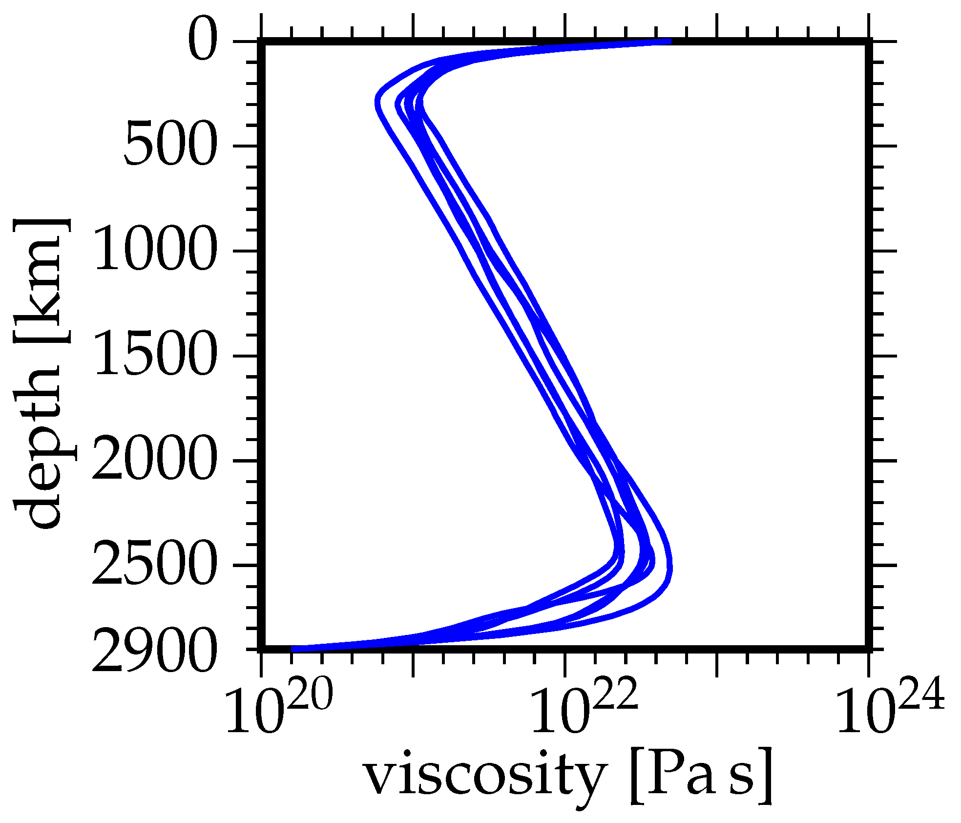
Figure 2.
Plots against elapsed time of the horizontal position of the continental lid for Cases 1–5. In the figure, () and () are the minimum and maximum values of , respectively.
Figure 2.
Plots against elapsed time of the horizontal position of the continental lid for Cases 1–5. In the figure, () and () are the minimum and maximum values of , respectively.

Figure 3.
Plots against elapsed times of (a) root-mean-squared velocities in the entire domain (red), along the top surface (green), and the absolute drifting velocity of the continental lid and (b) the horizontal coordinate of the center of the continental lid for Case 2. For the plot of in (a), the solid line indicates (namely, increases with time), while the dashed line indicates (namely, decreases with time). In (b), the shaded region indicates the range of the horizontal coordinate where the continental lid covers ().
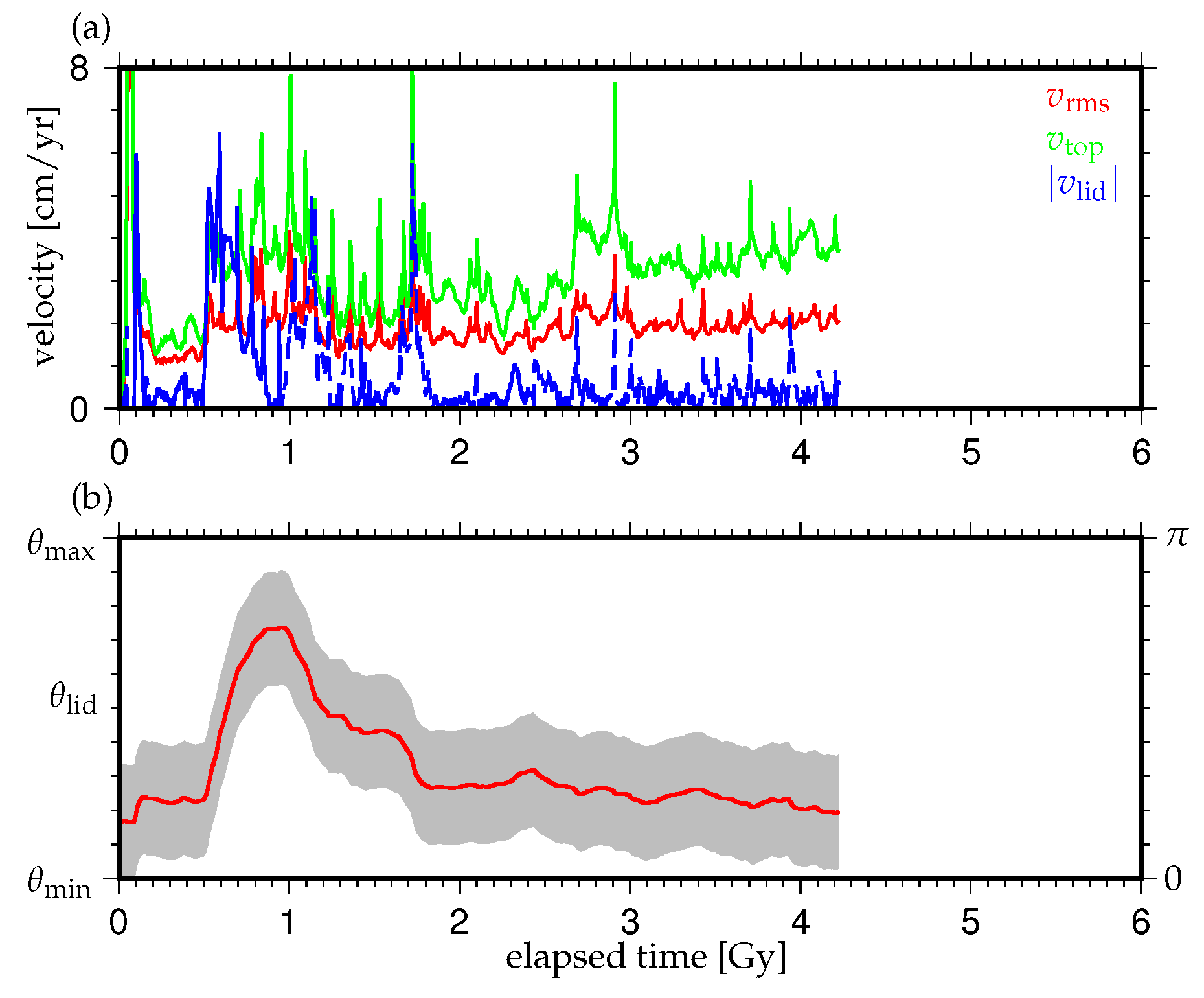
Figure 4.
Snapshots of the thermochemical states of Case 2 at the elapsed times indicated in the figure. Shown by color and contour lines in each row are the distributions of fraction c of the dense component (left) and temperature T (right). For the color scale for the distributions of c and T, see the scale bars in the figure. In each figure, the thick white lines indicate the positions of the continental lid at the top surface. Note that the mirror symmetry at the side walls ( and ) is assumed in displaying the distributions of c and T: in each snapshot is located at its top, while is at its bottom, and increases from to in clockwise and counterclockwise directions in the snapshots of composition c and temperature T, respectively.
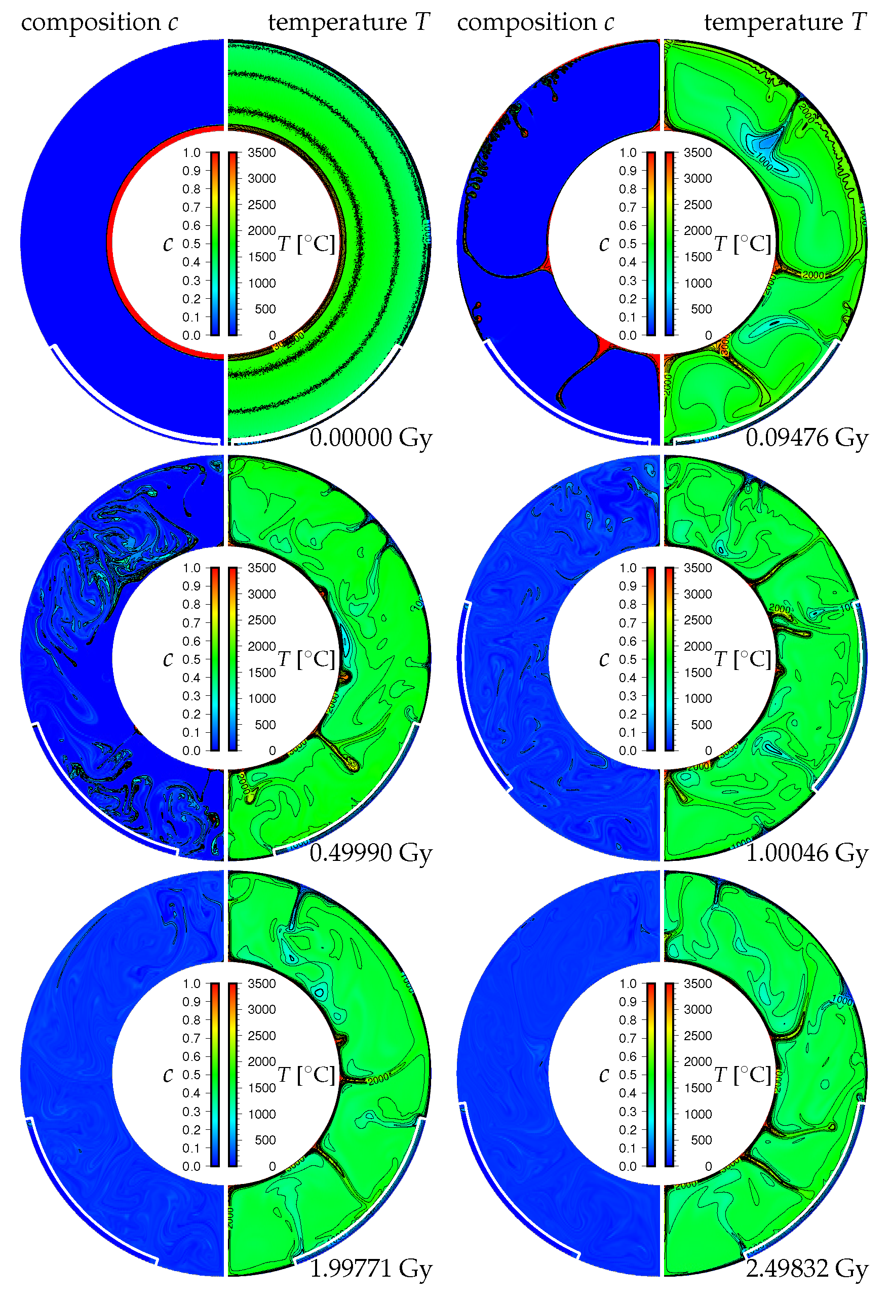
Figure 5.
Same as Figure 3, but for Case 3.
Figure 5.
Same as Figure 3, but for Case 3.
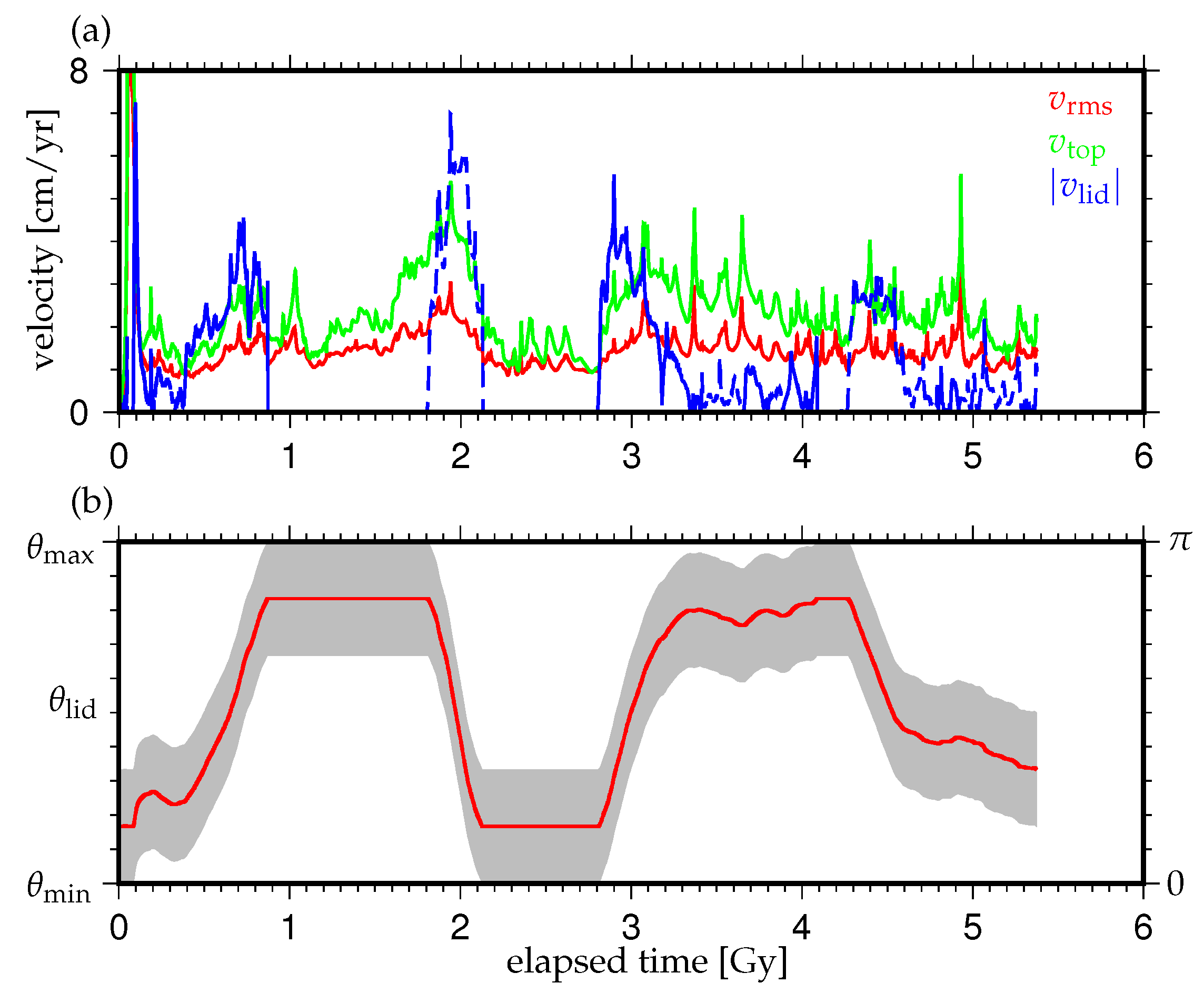
Figure 6.
Same as Figure 4, but for Case 3.
Figure 6.
Same as Figure 4, but for Case 3.
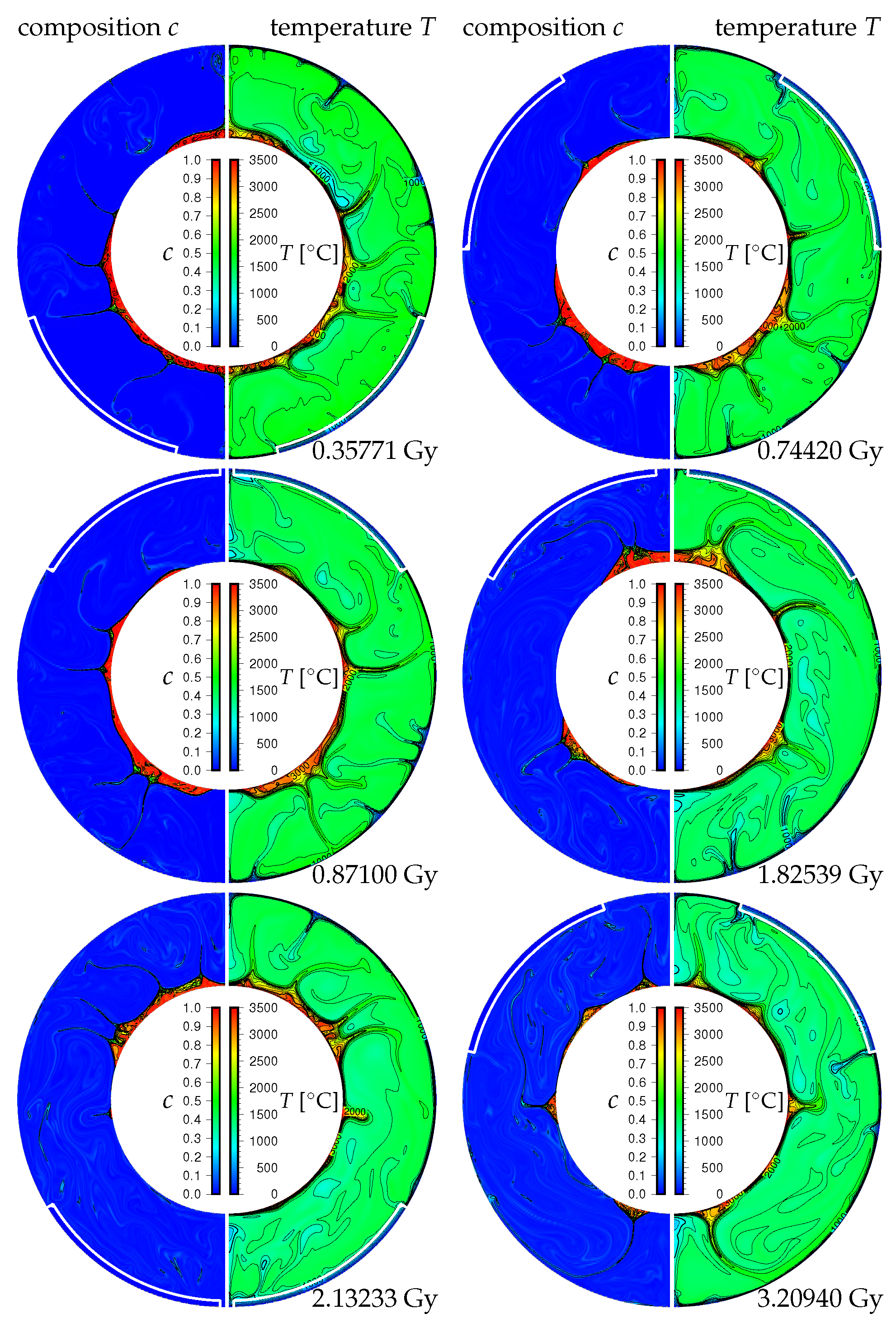
Figure 7.
Comparison of the snapshots of the thermochemical states of Cases 2 and 3 at the elapsed times indicated in the figure. Shown by color and contour lines in the first row of each column are the distributions of fraction c of the dense component (top left) and temperature T (top right). The meanings of the colors and thick white lines are the same as in Figure 4. Shown in the second row of each column are the distributions of dimensionless buoyancy coming from the differences in T and c at given depth (bottom right) and its radial profiles in the depth ranges below 1000 km from the top surface (bottom left). For the color scales for the distributions of , see the scale bars in the figure. In the plots of the bottom left of each row, the red and blue lines indicate the maximum and minimum values of at given depth, respectively, while the shaded regions delineate the standard deviation of at the depth.

Figure 8.
Temporal evolution as a function of the horizontal coordinate of composition c averaged over a (=181.25 km) depth just above the bottom surface for Case 4. For the color scale for the distributions of c, see the scale bar in the right of the figure. The two black lines indicate the positions of the margins of the continental lid as a function of the elapsed time (i.e., ), while purple dots indicate the positions of cold descending flows at the top surface for given elapsed times. See the text for the meanings of the labels “P”–“P”, “p”–“p” and “d”–“d”.

Figure 9.
Snapshots of the thermochemical states of Case 4 at the elapsed times indicated in the figure. In the snapshots both for the distributions of composition c and temperature T, the purple arrows indicate the velocity vectors and thin black lines are the iso-lines of temperature T. The meanings of the colors and thick white lines are the same as in Figure 4. See the text for the meanings of the regions labeled “P”–“P”, “p”–“p” and “d”–“d”.
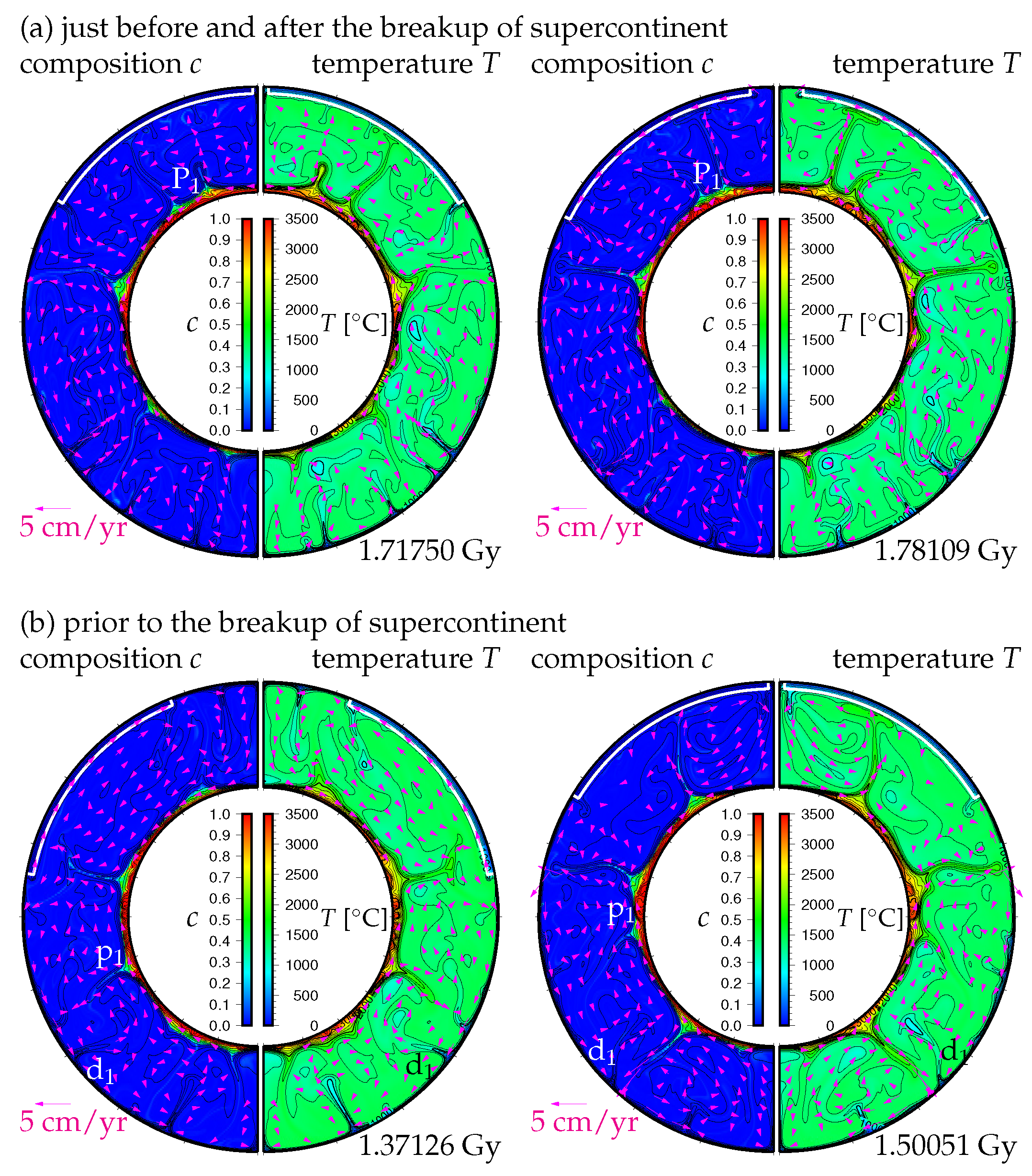
Figure 10.
Same as Figure 2, but for Cases 3C to 5C where the continental lid is initially positioned at the center of the top surface ().
Figure 10.
Same as Figure 2, but for Cases 3C to 5C where the continental lid is initially positioned at the center of the top surface ().

Figure 11.
Same as Figure 4, but for Case 6.
Figure 11.
Same as Figure 4, but for Case 6.
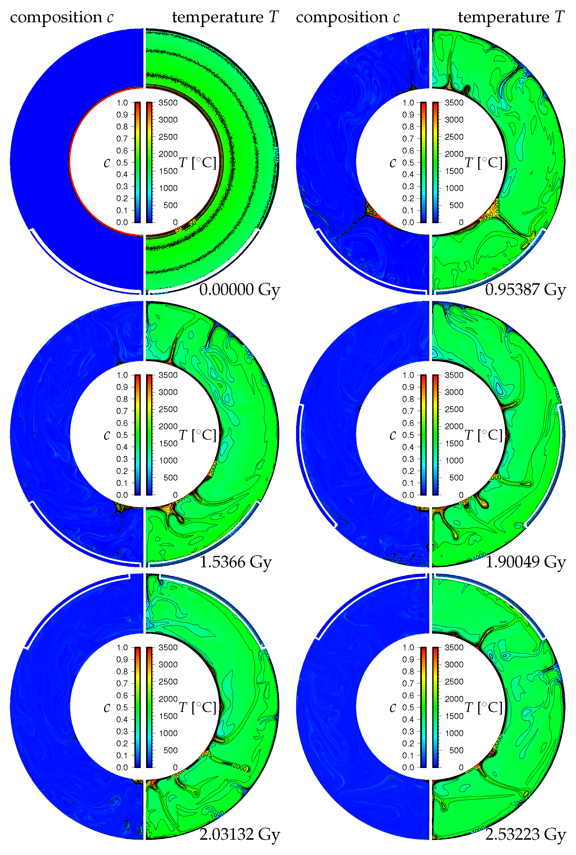
Figure 12.
Same as Figure 2, but for Cases 7–9.
Figure 12.
Same as Figure 2, but for Cases 7–9.

Figure 13.
Same as Figure 3, but for Case 7.
Figure 13.
Same as Figure 3, but for Case 7.
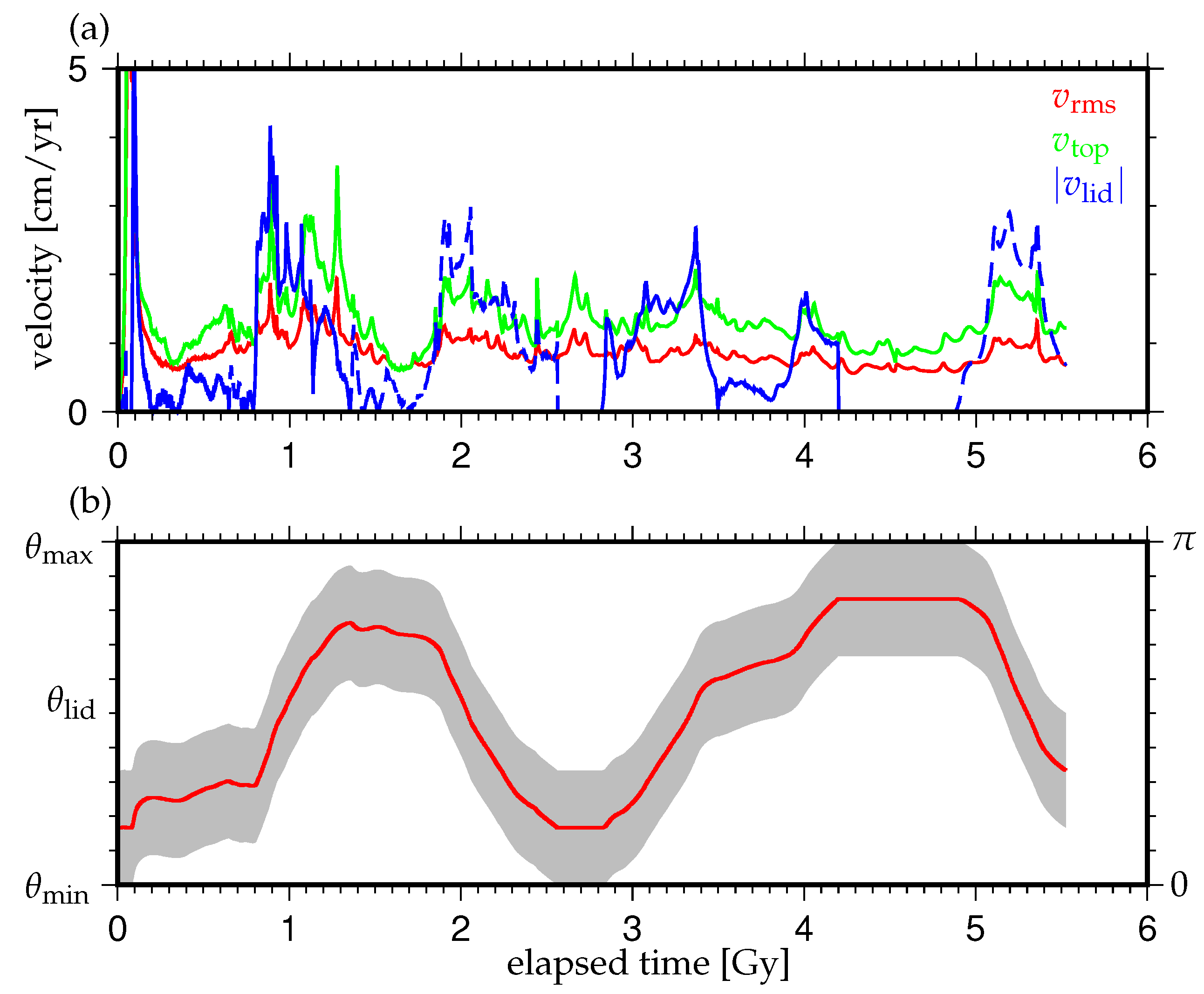
Figure 14.
Same as Figure 4, but for Case 7.
Figure 14.
Same as Figure 4, but for Case 7.


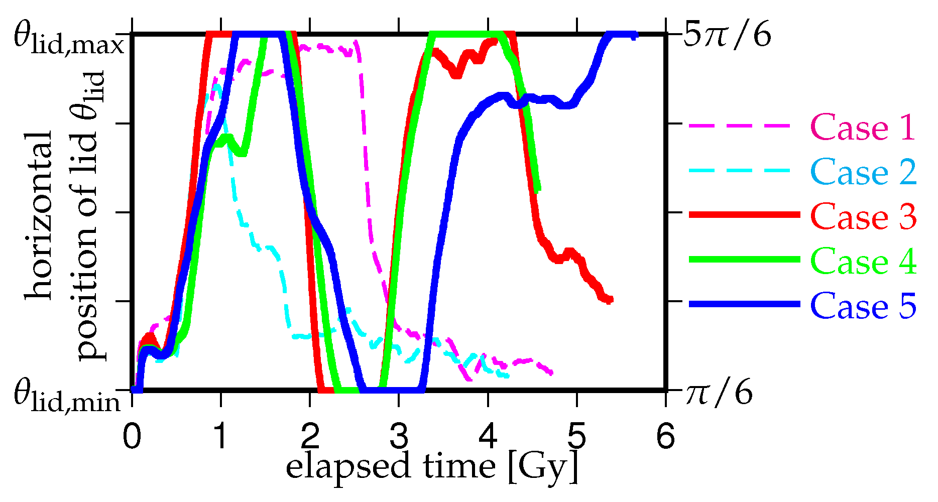
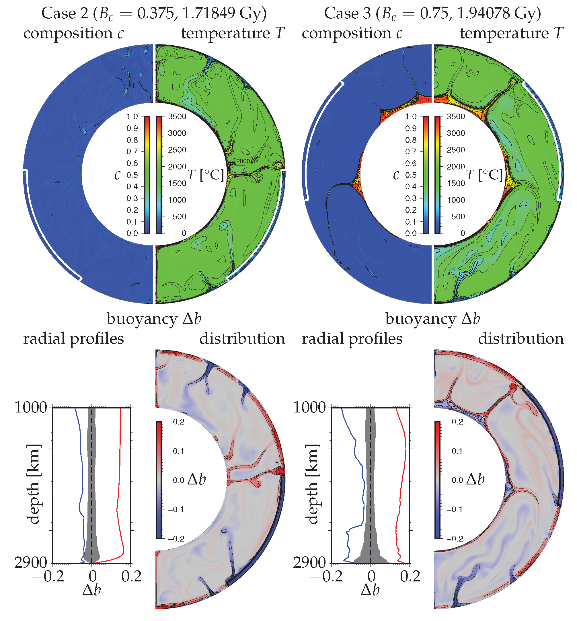
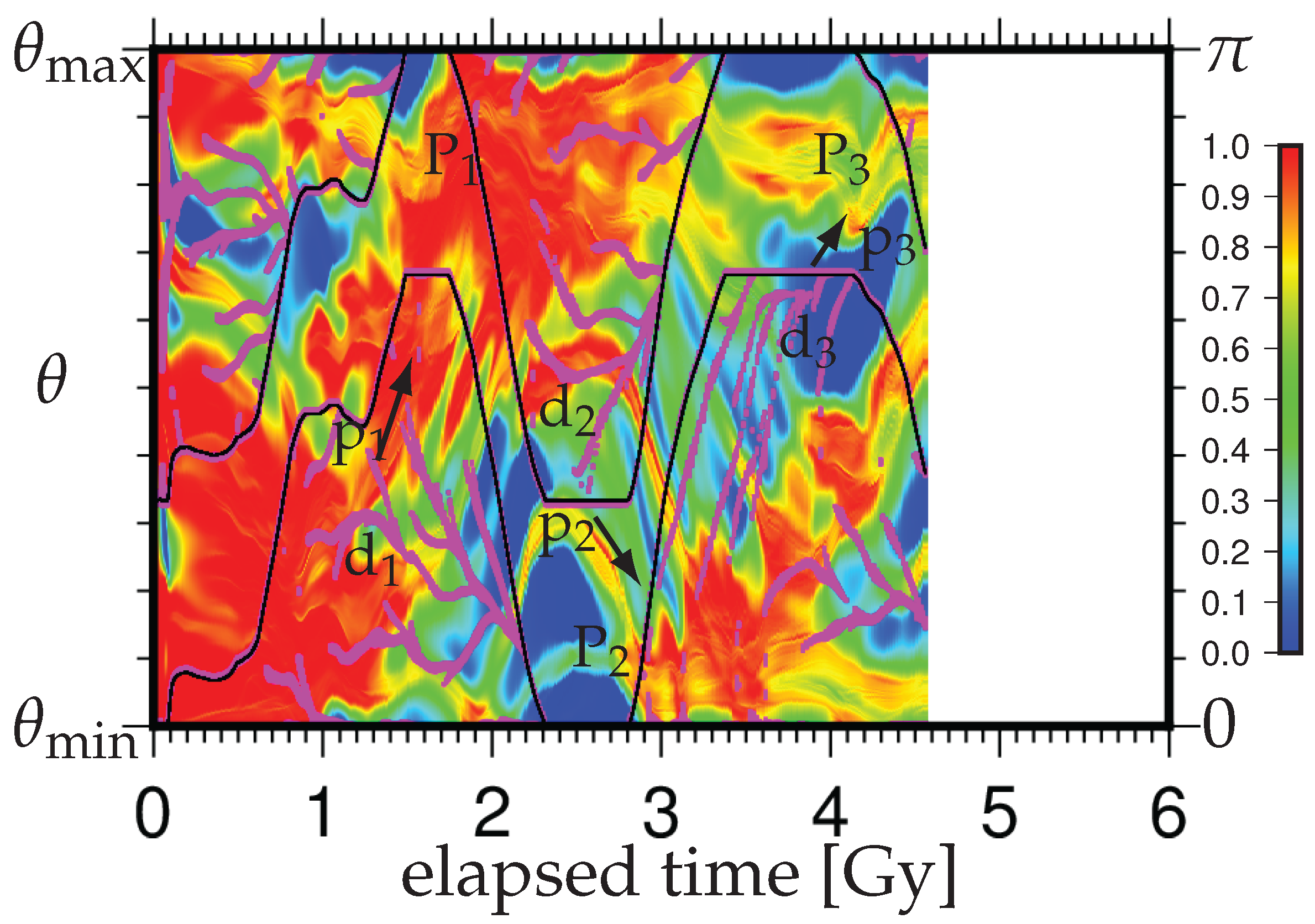
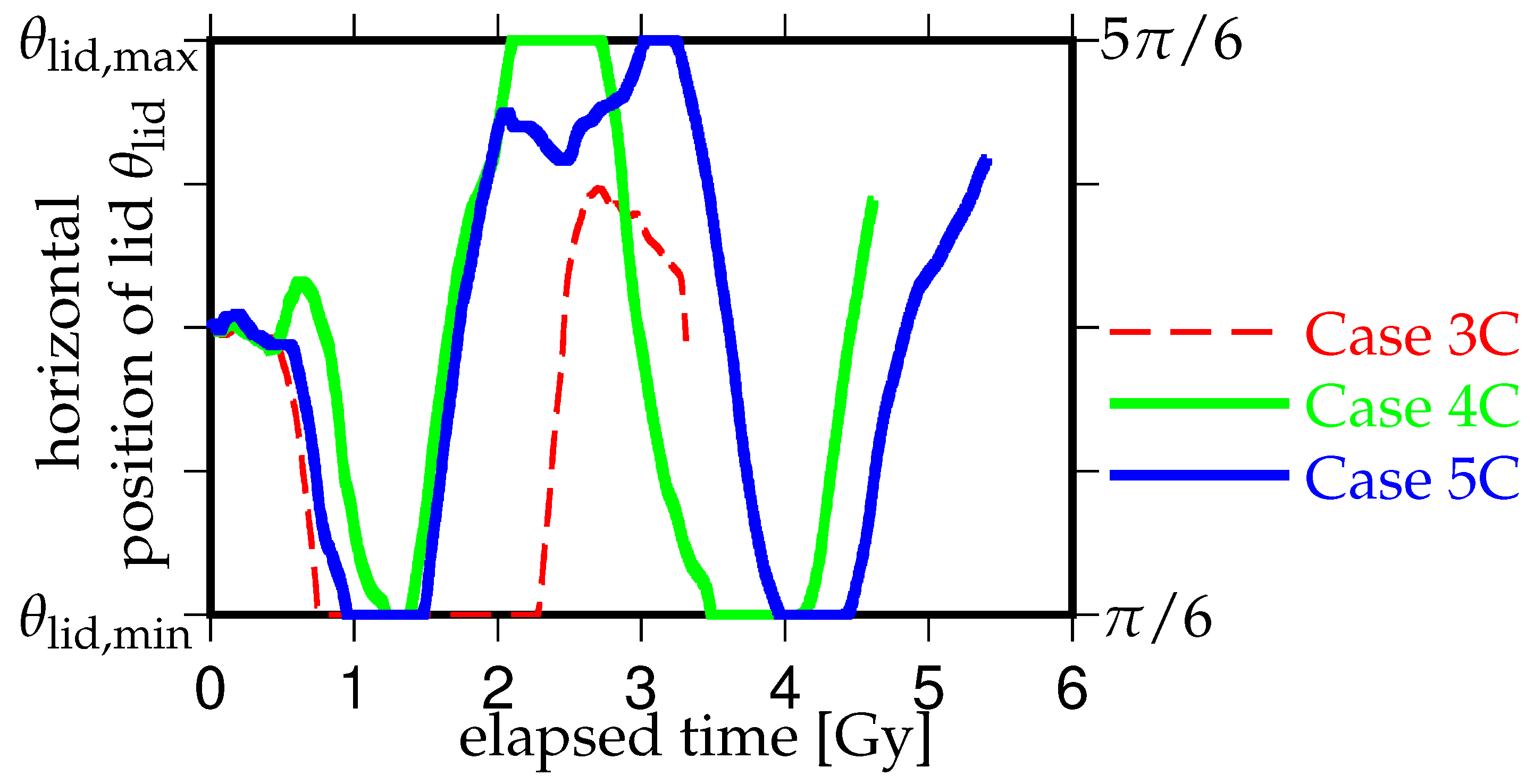
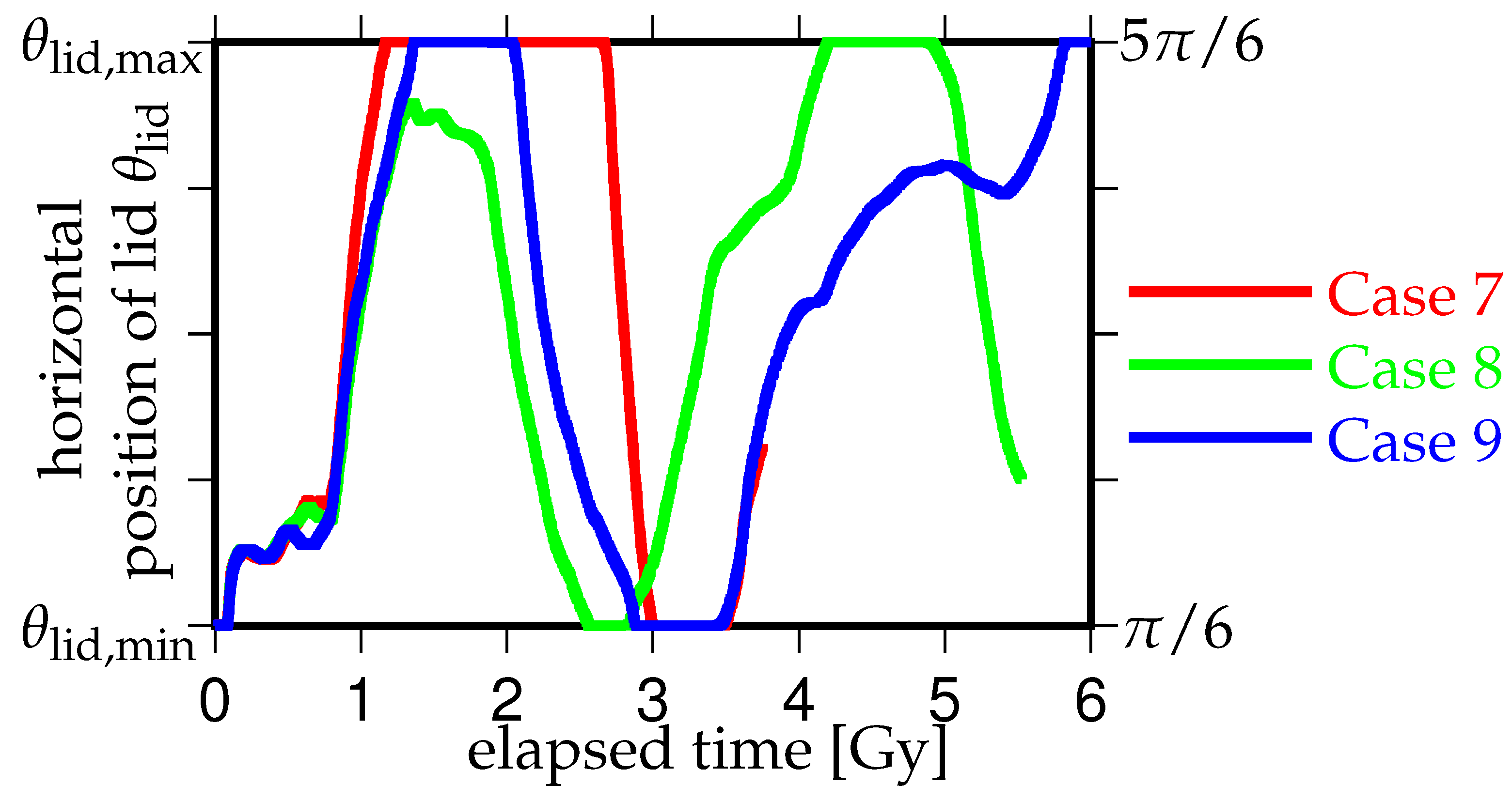
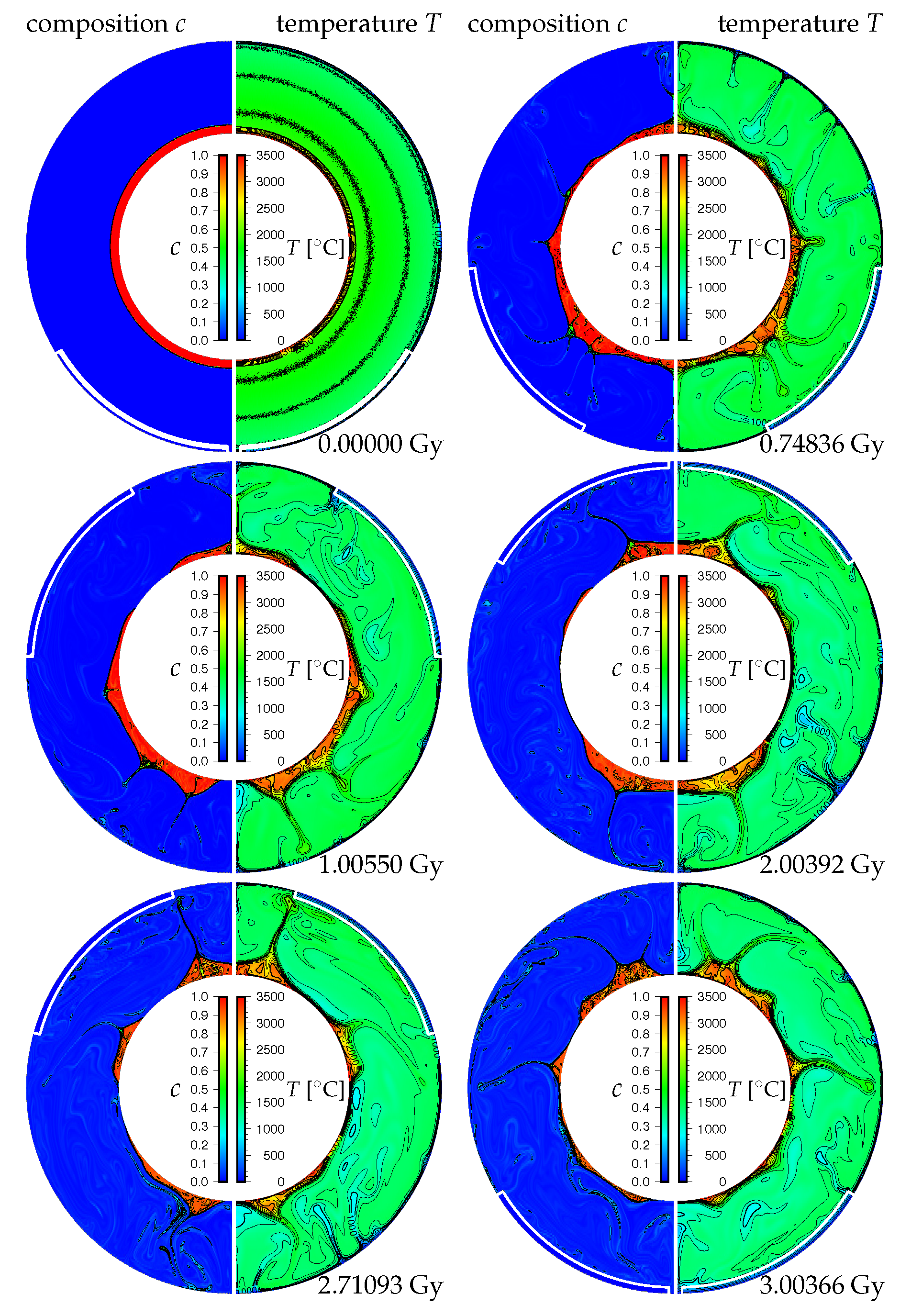
Table 1.
Adopted values of parameters.
| Symbols | Meanings | Values |
|---|---|---|
| density of Component A (“normal” mantle) | kg/m | |
| temperature difference across the mantle | 3500 K | |
| thickness of the mantle | m | |
| thermal expansivity | K | |
| specific heat | J/kg K | |
| viscosity | Pa s | |
| thermal diffusivity | m/s | |
| g | gravitational acceleration | m/s |
| Clapeyron slope of phase change at around 660 km depth | MPa/K |
Table 2.
The values of parameters and adopted for the calculations in this study.
| Cases | ||
|---|---|---|
| 1 | 0 | |
| 2 | ||
| 3 | ||
| 4 | ||
| 5 | ||
| 6 | ||
| 7 | ||
| 8 | ||
| 9 |
© 2017 by the authors. Licensee MDPI, Basel, Switzerland. This article is an open access article distributed under the terms and conditions of the Creative Commons Attribution (CC BY) license (http://creativecommons.org/licenses/by/4.0/).
Share and Cite
MDPI and ACS Style
Kameyama, M.; Harada, A. Supercontinent Cycle and Thermochemical Structure in the Mantle: Inference from Two-Dimensional Numerical Simulations of Mantle Convection. Geosciences 2017, 7, 126. https://doi.org/10.3390/geosciences7040126
AMA Style
Kameyama M, Harada A. Supercontinent Cycle and Thermochemical Structure in the Mantle: Inference from Two-Dimensional Numerical Simulations of Mantle Convection. Geosciences. 2017; 7(4):126. https://doi.org/10.3390/geosciences7040126
Chicago/Turabian StyleKameyama, Masanori, and Akari Harada. 2017. "Supercontinent Cycle and Thermochemical Structure in the Mantle: Inference from Two-Dimensional Numerical Simulations of Mantle Convection" Geosciences 7, no. 4: 126. https://doi.org/10.3390/geosciences7040126
Note that from the first issue of 2016, this journal uses article numbers instead of page numbers. See further details here.