Article

Semi-Automatic Detection of Indigenous Settlement Features on Hispaniola through Remote Sensing Data

by
Till F. Sonnemann
1,*,
Douglas C. Comer
2,
Jesse L. Patsolic
3,
William P. Megarry
4,
Eduardo Herrera Malatesta
5 and
Corinne L. Hofman
5
1
Institute of Archaeology, Heritage Sciences and Art History (IADK), Otto-Friedrich-Universität Bamberg, Am Kranen 14, 96047 Bamberg, Germany
2
Cultural Site Research and Management (CSRM), 2113 St. Paul Street, Baltimore, MD 21218, USA
3
Center for Imaging Science, Johns Hopkins University, Baltimore, MD 21218, USA
4
School of Natural and Built Environment, Queen’s University Belfast, Belfast BT7 1NN, UK
5
Faculty of Archaeology, Universiteit Leiden, Einsteinweg 2, 2333 CC Leiden, The Netherlands
*
Author to whom correspondence should be addressed.
Geosciences 2017, 7(4), 127; https://doi.org/10.3390/geosciences7040127
Submission received: 15 October 2017 / Revised: 29 November 2017 / Accepted: 29 November 2017 / Published: 5 December 2017
(This article belongs to the Special Issue Remote Sensing and Geosciences for Archaeology)

Abstract

:
Satellite imagery has had limited application in the analysis of pre-colonial settlement archaeology in the Caribbean; visible evidence of wooden structures perishes quickly in tropical climates. Only slight topographic modifications remain, typically associated with middens. Nonetheless, surface scatters, as well as the soil characteristics they produce, can serve as quantifiable indicators of an archaeological site, detectable by analyzing remote sensing imagery. A variety of pre-processed, very diverse data sets went through a process of image registration, with the intention to combine multispectral bands to feed two different semi-automatic direct detection algorithms: a posterior probability, and a frequentist approach. Two 5 × 5 km2 areas in the northwestern Dominican Republic with diverse environments, having sufficient imagery coverage, and a representative number of known indigenous site locations, served each for one approach. Buffers around the locations of known sites, as well as areas with no likely archaeological evidence were used as samples. The resulting maps offer quantifiable statistical outcomes of locations with similar pixel value combinations as the identified sites, indicating higher probability of archaeological evidence. These still very experimental and rather unvalidated trials, as they have not been subsequently groundtruthed, show variable potential of this method in diverse environments.

Graphical Abstract

1. Introduction

The fascination with feature identification and mapping of geometric archaeological alignments by means of remote sensing is as old as the first appearance of aerial photos [1,2,3]. Throughout the last centuries, it has advanced significantly, leading to new archaeological discoveries using imagery from satellites and drones [4,5]. The human eye remains an adept feature extractor and can distinguish linear or circular structures and earthworks easily from the natural soil [6]. More recently, however, automatic approaches in pattern recognition have also become common, often based on computer algorithms adopted from other disciplines [7,8,9,10], and tested for archaeological purposes to detect color [11,12], changes in topography [13,14] or different reflection patterns [15].
A different challenge is the identification of non-geometric archaeological features with more amorphous shape and structure. Without any clear geometry they pose a special problem, as the most prominent parameter for successful recognition is missing. This is the case for indigenous settlements in the Caribbean, which have been identified through assemblages of shells, ceramics bone remains, and stone tools; but not by traces of extant or sub-surface structural remains [16,17]. The irregular pattern of pre-colonial settlement vestiges has made their detection challenging for remote sensing [18]. Previous work has been dominated by traditional archaeological survey methods: the identification of surface material based on the knowledge of local scouts or landowners, and defining an approximate delineation of areas based on the surface finds on site [19,20]. The trial approach presented here, a methodological experiment exploring the use of various datasets and approaches, rather than providing any validated method or results, is nevertheless an example for a novel statistical, systematic, and therefore more objective method.
The posterior probability and the frequentist approach are two algorithms developed at Cultural Site Research and Management (CSRM) [21,22] as a Direct Detection Model (DDM), to identify the probability of sites by comparing single pixel values. Both algorithms were modified at the time of the study and ready for use at different times; this is one reason why each was applied on a different trial area. The general idea behind direct detection is that anthropogenic activities at archaeological sites, often over long periods of time, have impacted these parts of the landscape in ways that if they persist are statistically measureable in remote sensing data. The DDM has therefore two sets of input data. The first set has two parts. One is the locations of known archaeological sites. In the trial area of the northwestern Dominican Republic and Haiti, the archaeological “sites” were identified over several years by different archaeologists, mostly with the help of local guides. Each site visited was named, a number of archaeological samples taken, and georeferenced by taking one or more GPS points at the site using a handheld device. In addition the algorithm needs areas, at best also groundtruthed, with presumably no sites, which are equally important for the study. A second data set comprises a variety of remote sensing imagery. The subtle variation between already discovered areas of human activity, the sites, and areas of no human activity (non-sites) within each remote sensing band, can be used to detect difference. The difference is more likely to be detected when many different bands of available satellite or aerial data sets are combined.
The area of interest, northern Hispaniola, presents a highly diverse environment. Along the coast runs the 200 km long Cordillera Septentrional, a several hundred meter high mountain range, partly covered by temperate to tropical forest, separating the coast from the fertile floodplain of the Valle de Cibao. Large parts of the hills and the plains north of the cordillera have been cleared for pasture. The northern coast is protected by coral reefs and mangrove forests. The region has been settled through waves of immigrations, archaeologically divided into earliest lithic age period since 4000 BC [23], the archaic period from 2500 BC the later ceramic ages distinguishable by ostionoid, meillacoid and chicoid ceramics [23,24,25,26]. Shortly after the arrival of Columbus, and the foundation of the first Spanish town in the Americas at La Isabella in 1493 [27], evidence for Amerindian activity declines rapidly [28] from the archaeological record [29,30]. We can therefore postulate that most sites marked in the map are either from prehistoric or very early colonial times. Variations in topography, land use and vegetation have created a landscape that changes over few kilometers, which also affected the indigenous settlement strategy [31]. Accumulations of shells indicate Amerindian use of marine resources [32], while other sites, often on prominent location overseeing the landscape, have been identified as settlements due to their particular topographic attributes consisting of mounds and flattened areas that served as base for house construction [30,33,34].

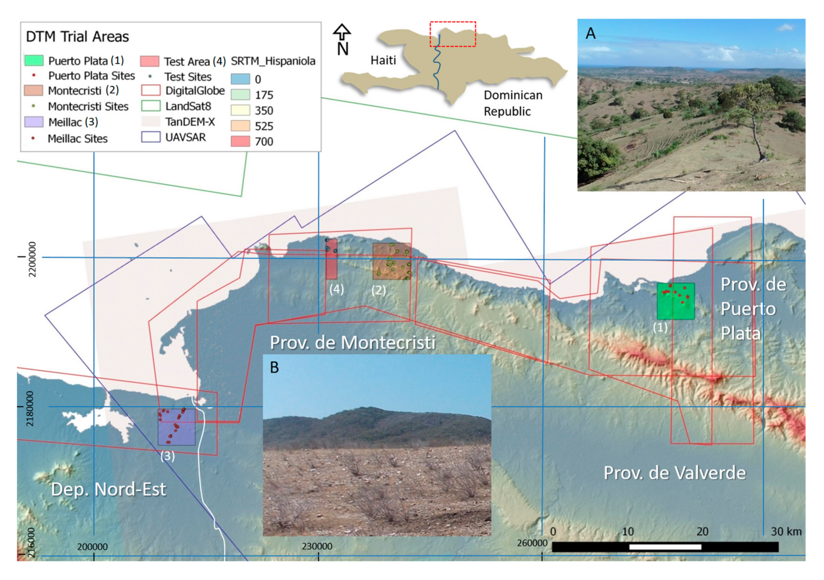
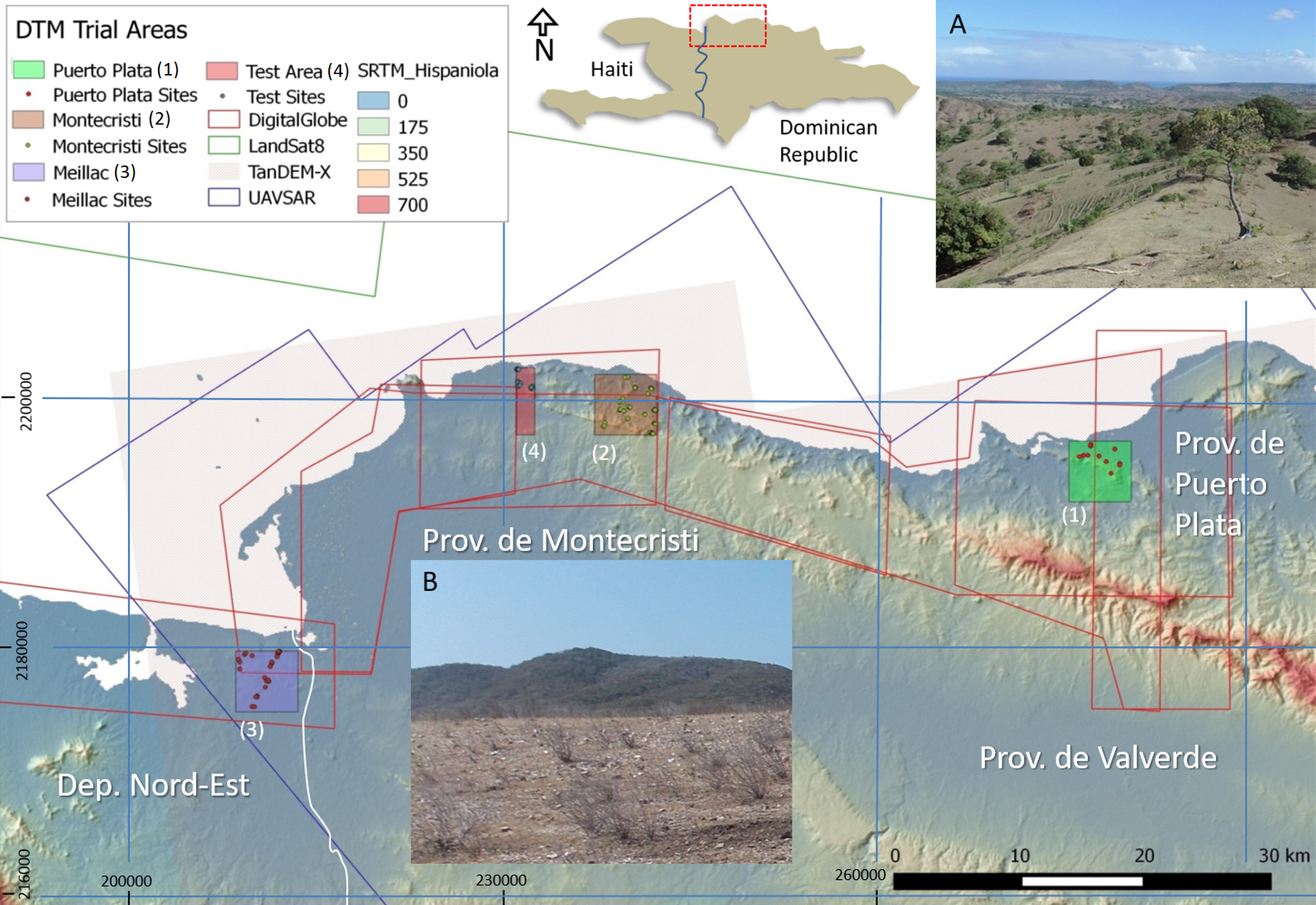
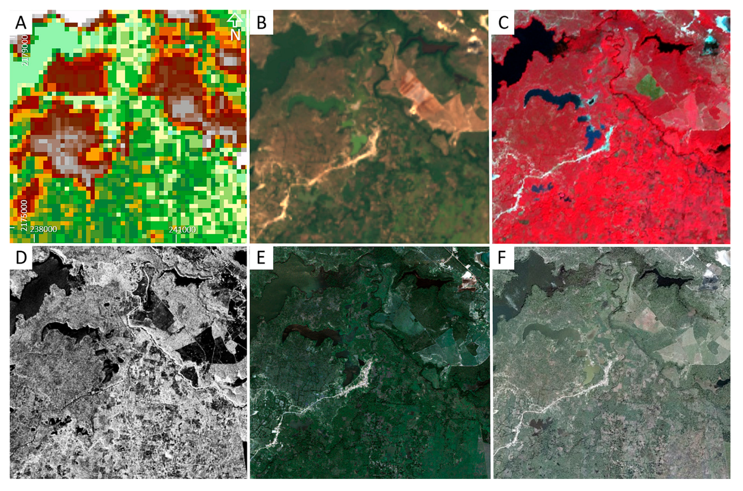
2. Materials and Methods
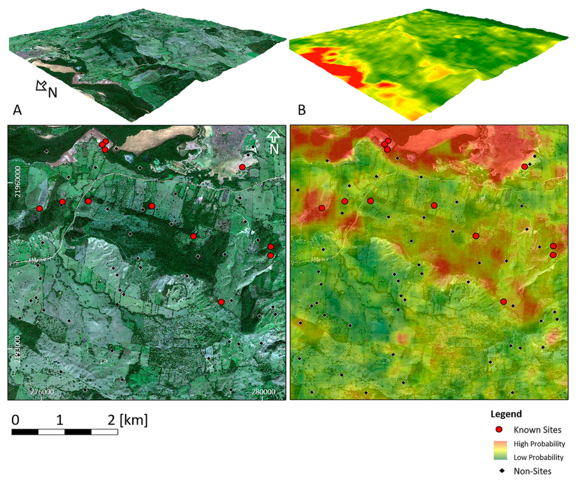
Based on the availability of remote sensing datasets, and samples of already identified archaeological sites, three areas of 5 × 5 km2 in different environments were initially identified for trials. All existing archaeological site datasets were merged into a single point shape file, and then split for each of the trial regions. Only the two areas in Puerto Plata, DR (1) and Montecristi, DR (2) were ultimately trialed (Figure 1). The third area in Meillac (Dep. Nord-Est), Haiti, (3) was excluded following the second round of trials. An additional 1.5 × 5 km2 area (4), which had been focus of a systematic total area survey [35], was initially thought to be well suited for comparing remote sensing and ground interpretation. Unfortunately, it had to be discarded, as there were not enough known sites in the area to be implemented in the algorithms, a universal issue of sample size when doing predictive models. Most of these techniques require thousands of points in other areas to compare, particularly for the small region impossible to provide.
The passive remote sensing data sets Landsat-8, Worldview-2, ASTER, and active sensors UAVSAR (Uninhabited Aerial Vehicle Synthetic Aperture Radar) as well as TanDEM-X stripmap (see Table 1 and Figure 2) were chosen based on resolution, availability, accessibility and practicality; they were either freely available, or acquired through generous data grants. Aerial imagery of northern Haiti was provided free of charge by Haiti’s Centre National de l’Information Géo-Spatiale. Atmospherically corrected 15 m ASTER (Advanced Spaceborne Thermal Emission and Reflection) data was acquired through NASA/METI/AIST/Japan Space Systems and US/Japan ASTER Science Team, the low resolution however made the imagery of limited use. Additionally, several TanDEM-X data sets were acquired through a research license agreement with the DLR e.V. (Project: OTHER6189, https://tandemx-science.dlr.de/), but ultimately the uncorrected data was not utilized for the DDM. All other remote sensing data went through a series of image registration protocols to render them standard in pixel size, resolution and angle that allowed exact correlation between pixels of different data sets. To achieve this goal, all datasets were initially converted to the same georeferenced system: WGS 84, UTM 19N for the Dominican Republic (20N respectively for Haiti). Because of insufficient spatial resolution, work with Landsat-8, and ASTER was discontinued after consideration, leaving UAVSAR and Worldview-2 for further steps. The latter, multispectral data set, made available by the DigitalGlobe Foundation, covers the regions of interest in two-meter-resolution with one panchromatic and eight multispectral bands (see Table 2). The data set, with bands in the visible and near-visible range, was atmospherically corrected to reflectance values [36]. This standardized imagery removing artefacts caused by atmospheric interference. While often neglected, atmospheric correction is important and can significantly impact subsequent processing techniques like indices [37].
From the original Worldview-2 data, the transformations NDVI, PCA and Tasseled Cap were applied in ArcGIS 10.3 (ESRI, Redlands, CA, USA), with the purpose to create additional bands that may improve the site identification regarding their environmental discrimination. Of these, the NDVI (Normalized Difference Vegetation Index) [38] is a unidimensional spectral index, adjusting the band information based on the principle that healthy vegetation absorbs most of the visible light and reflects most of the near-infrared light. Unhealthy or sparse vegetation reflects more visible light and less near-infrared light. The formula applied (1) used the bands red (visible) and red edge (to represent near-infrared):
NDVI: Float (“Red Edge“ − “Red”)/(“Red Edge” + “Red”)
Principal Component Analysis (PCA) was applied with the intention to reduce the data dimensionality of correlated bands [39]. The method rotates the original space of features into a new space where the transformed features are pairwise orthogonal. This creates an n-dimensional space of eigenvectors, where n is the number of input dimensions (features), with the goal to orthogonalize the data set. The first principal component accounts for the maximum proportion of variance from the original dataset, the following, being orthogonal to the first one, for the next principal components, creating eventually a new coordinate system of orthogonal axes. A subset of the components is usually chosen for subsequent analysis. The method used to select these components varies by application. The first three components were included in the algorithm while the latter components were discarded as redundant. For a more detailed explanation, see [40].
Tasseled Cap Transformation or K-T (Kauth-Thomas) transform (KTT), as originally developed by [41] for LandSAT imagery, was applied on each Worldview-2 data set using bands one to eight in accordance with [42]. Tasseled cap applies predefined correction coefficients to each band and will produce eight new bands. This spectral index conversion intends to highlight changes in vegetation and soil, where the pixel values are being transferred into a new orthogonal axial system; of these the first three new bands are the most important, representing Brightness (red) (2), Greenness (green) (3) and Wetness or yellowness of vegetation (blue) (4). Based on the reflectance values given by [42] for each Worldview-2 component, the formulas go as such:
Brightness: Float (0.060436 × “Coastal” + 0.012147 × “Blue” + 0.125846 × “Green” + 0.313039 × “Yellow” + 0.412175 × “Red” + 0.482758 × “Red Edge” − 0.160654 × “NIR1” + 0.67351 × “NIR2”)
Greenness: Float (−0.140191 × “Coastal” − 0.206224 × “Blue” − 0.215854 × “Green” − 0.314441 × “Yellow” − 0.410892 × “Red” + 0.095786 × “Red Edge” + 0.600549 × “NIR1” + 0.503672 × “NIR2”)
Wetness and Shadow: Float (−0.270951 × “Coastal” − 0.315708 × “Blue” – 0.317263 × “Green” − 0.242544 × “Yellow” − 0.256463 × “Red” − 0.096550 × “Red Edge” − 0.742535 × “NIR1” + 0.202430 × “NIR2”)
NASA had captured UAVSAR (Uninhabited Aerial Vehicle Synthetic Aperture Radar) polarimetric L-band data of ~5.7 m, over the large fault zones of Hispaniola. Publicly available, this data set also covers the areas of interest. Accessed through the JPL/ASF website, the data was extracted to single band TIFF-files using [43] (downloaded product: PolSAR-polarimetric SAR-MLC). Different materials reflect radar waves with different intensities and polarizations. Among the feature differentiated are smoothness, homogeneity, as well as soil moisture, and vegetation discrimination revealed by variation in density and structure. For polarimetric SAR image representation, the Pauli color-coding is a useful application to visually differentiate the three major scattering mechanisms (1) single bounce from a plane surface backscattered towards the radar, (2) double bounce from one flat surface that is horizontal with an adjacent vertical surface, and (3) volume scattering from randomly oriented scatterers [44]. From the original seven UAVSAR bands, Pauli decomposition bands were produced through a linear combination of HH, HV, VH and VV in one three-color RGB image [45] (see Table 3).
For each region, the chosen 5 × 5 km2 test areas were overlaid by a point grid of 2m-resolution, to create a matrix of 2500 × 2500 sampling pixels from each dataset (Figure 3). These values were then interpolated into a stack of registered raster dataset of the same 2 m resolution. After this transformation, the pixels and their attributes of each band overlapped exactly, diminishing the possibility of corner and border uncertainties. In addition, the prepared Worldview-2 data set served as base for land cover classification (Table 4), using sample regions for each attribute, made with the Image Classification toolbar of the Spatial Analyst extension in ArcGIS 10.3, to better distinguish the variety of surface coverage.

3. Results

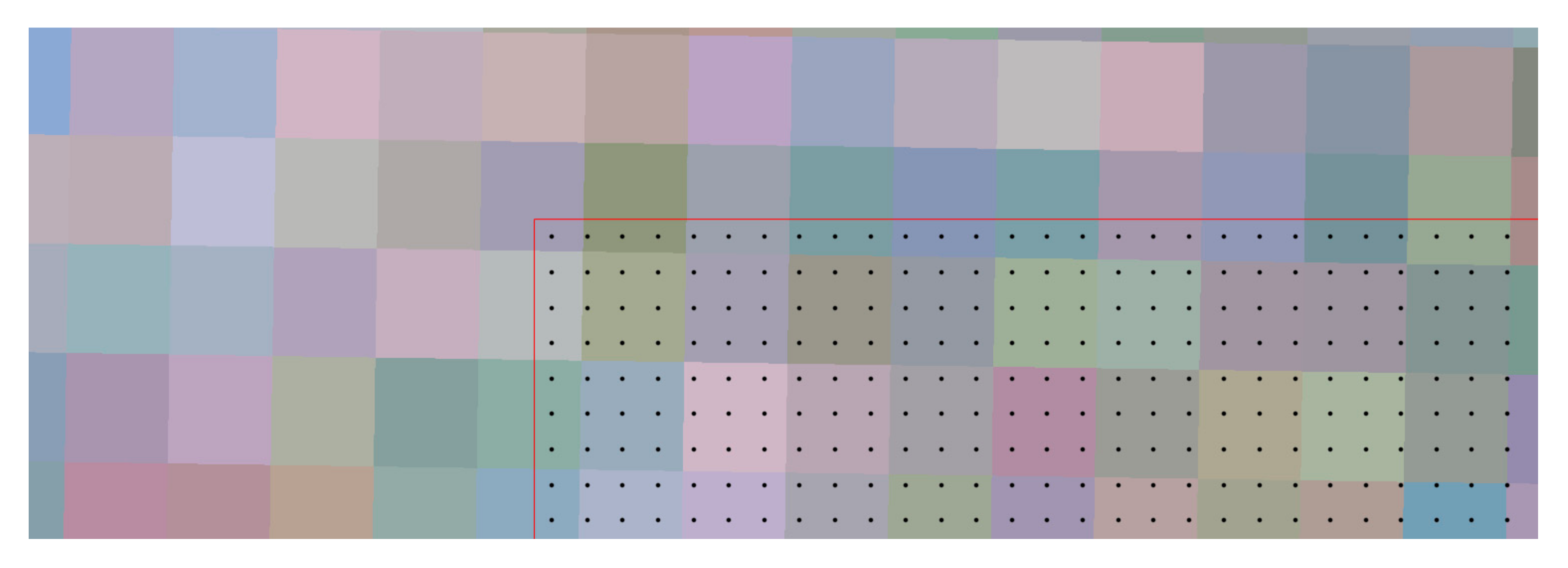
3.1. Posterior Probability Approach

Initial tests on a modified version of the algorithm, using a posterior probability modeling [46,47,48,49] to define difference between potential areas of sites and non-sites were conducted with focus on a trial area in Puerto Plata, DR. The model records posterior probabilities generated using a linear discriminant analysis (LDA) with a Bayes plug-in classifier. LDA assumes normal distributions with similar covariance conditional on the input classes. Probabilities record the likelihood of cells belonging to a specific class and thresholds can be used to create definitive classifications. While preferable in other areas, the ordinal scale of probability values are more useful when assessing the likelihood of sites as they represent the possibility of sites being present or not. This approach had been successfully applied elsewhere and involved using known sites and alleged non-sites to build a binary classifier where each cell was assigned a posterior probability of being an archaeological site. Datasets included Woldview-2 imagery and band difference ratios similar to the NDVI, which were then reduced using PCA. The sites in the original dataset were represented by single artifact find spots around a central point which represented the site proper. Polygons were digitized around all points to delineate sites. There were 12 sites in the area with an average area of 4338 m2. Non-Sites were generated according to the following rules:
  • in surveyed areas
  • A total of >100 m from known sites
  • Buffers with a radius of 37 m (with an area of 4300 m2) were generated around each site.
It was important that non-sites shared similar characteristics to actual sites, so the buffer size was chosen based on the average size of known sites in the area (4300 m2) as calculated by material scatters. The trial results were plotted on a ROC curve (Figure 4), which demonstrates that sites were much more likely to be found in the high or higher probability areas of the posterior probability maps of the Puerto Plata trial region, and much less likely in the low probability areas.
Considering the entered data sets, known sites were mostly located in the mangrove forest and on hilltops or slopes, while non-sites were distributed over the complete data set, the results showed a positive outcome, coloring similar locations in deep red (Figure 5). There are however two general caveats. Firstly, the algorithm based on a binary classification might be more effective when identifying homogenous site-types like lithic scatters. Secondly, the algorithm performed better with a larger and very accurate sample of known sites and checked known non-sites of a surveyed area. In this project, the heterogeneous nature of the sites coupled with a small number of known sites must be regarded as an impediment to this approach. When focusing on the research area, the approach may have also been hindered by the dominance of sites in the mangroves near the ocean shore, and on hilltops; the algorithm favored these areas for probable site locations. Considering the visual interpretation of the outcome by the archaeologists working in the region, and having recorded the known sites, the results generally make sense. Only based on the remote sensing imagery and without any topographic information, the highest probability of undiscovered sites is found near or on the hilltops’ northern side, where additional sites were to be expected, while the region south of the range of hills is void of any probable sites. This of course remains highly speculative and is only based on landscape understanding and survey experience, and could only be confirmed by an independent accuracy assessment applied onto a different, possibly larger area, or through additional ground truthing by a total area survey of the region. Because of the clustering of a relatively limited number of sites, the Puerto Plata area (1) was seen potentially unsuitable as a trial region, and the team decided to continue with the Monte Cristi area (2), which provided more known sites, that were more broadly distributed over the area, using a different approach.

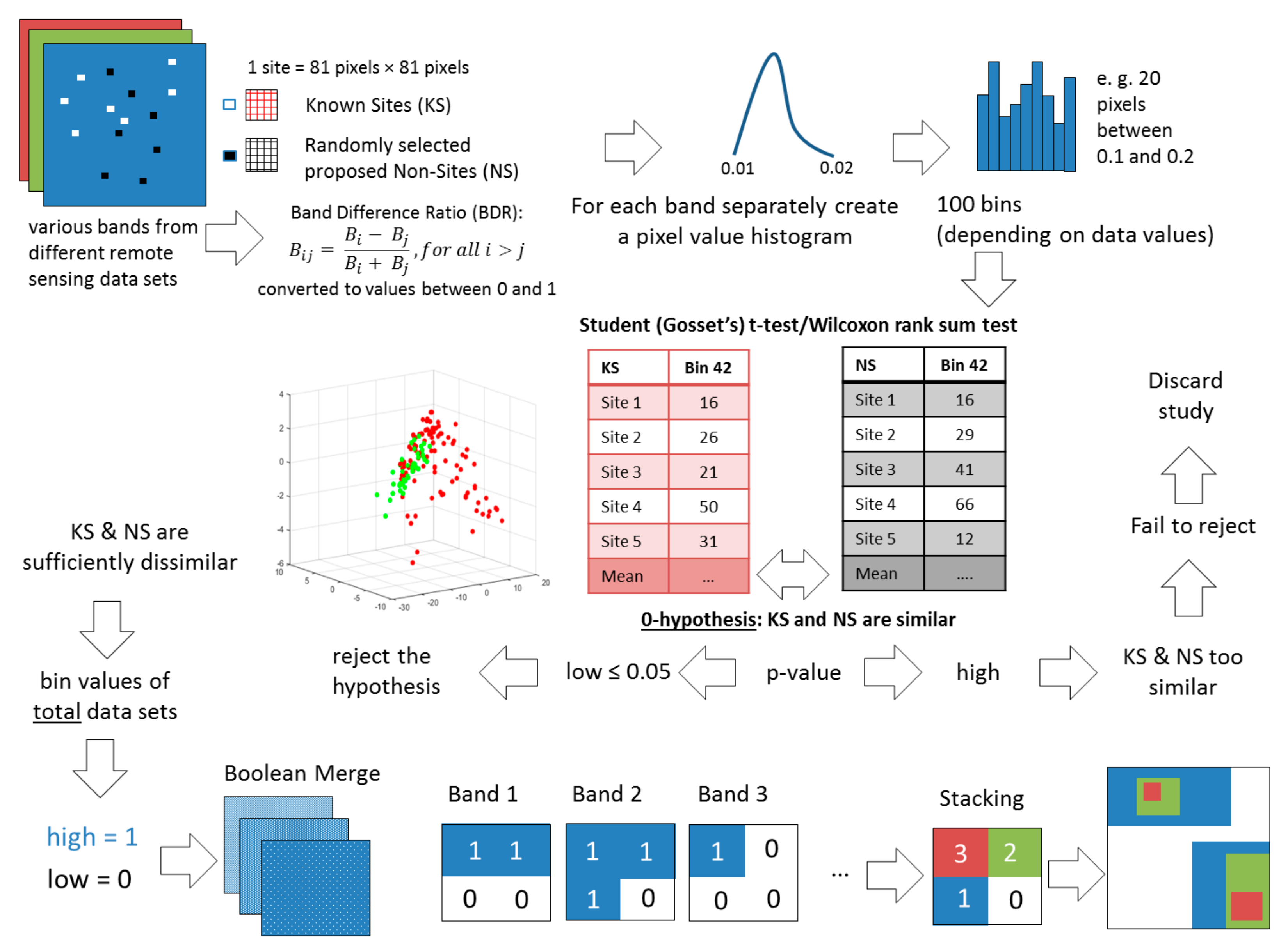
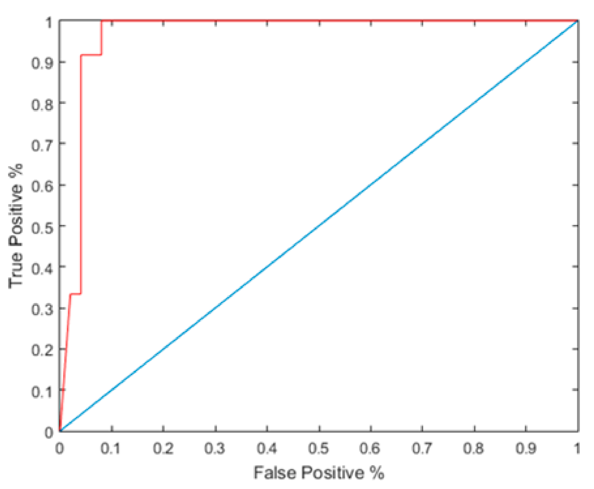
3.2. Frequentist Protocols

A frequentist [22] approach, programmed in the statistical Software R (R Foundation for Statistical Computing, Vienna, Austria) [50], was applied for the Montecristi area (Figure 6). This 5 × 5 km2 area is located in a hilly part of the coastal region of Montecristi, where new sites had recently been identified [31,35,51], of which 16 sites were chosen. A window of 81 pixels × 81 pixels (160 × 160 m2) was set around the single pixels picked as the center of the known sites (KS) and randomly selected non-sites (NS) creating a base of information of 6561 pixels, across each band, for each point of interest. The same number of known sites and non-sites was considered. Histograms were generated for each separate band across sites and non-sites. The histograms were binned in 100 equally spaced separations (see Figure 7). A student t-test/Wilcoxon rank sum test was conducted to see if there is a significant dissimilarity between sites and non-sites.
A variety of statistical explorations were conducted. A band-difference ratio (BDR) was generated between all pairs of bands. Given two bands, their BDR is given by the pixel-wise quotient of their difference over their sum. This procedure is exactly the same as NDVI, but additionally utilizes all unique pairs of bands. The original bands (WV2) are used along with these new BDR bands in the analysis, which is performed on the WV2 bands and then the BDR bands. For each band, the 81 pixels × 81 pixels extents of KS and NS are extracted, separately. The KS pixels and NS pixels are binned respectively using the same bin widths. The KS and NS pixels in each paired bin are compared in a hypothesis test with null hypothesis that the KS pixels and NS pixels are of the same distribution. If we fail to reject the null hypothesis at significant level 0.05, then that bin is marked 0; otherwise it is marked 1. This creates a binary matrix for each of the bands. A Boolean merge is then applied, that is, these matrices are summed together.

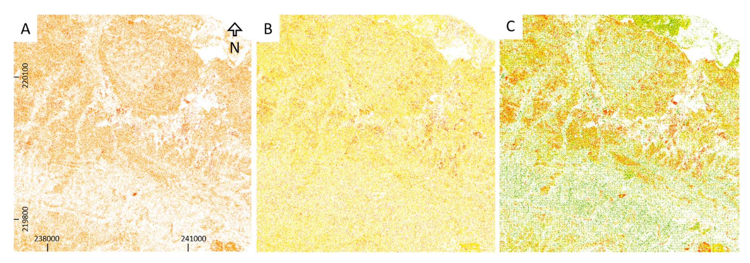
3.3. Dominance of Bands

A variety of statistical trial calculations were applied. A band-difference ratio (BDR) was generated among every band included in the algorithm data set, to reduce the dominance of particular, as well as essentially redundant, data sets. These ratios were indices similar to the NDVI and normalized datasets. Only bands with the lowest positive response rate, a low p-value (cause for rejecting the 0-hypothesis that KS and NS were similar) were further considered for the tests. The highly diverse environment, as made visible in the land cover maps, would, one might expect, influence the success of the approach in comparison with other areas where land cover was more homogenous [52].
The frequentist protocol from [21,52] was implemented in R with different binning strategies [53,54] using Student’s (Gosset’s) T-Test or the Wilcoxon rank sum test (for explanations of these tests, see [55]). The bulk of the work in R was done as exploratory data analysis with mixing and matching binning strategies and hypothesis testing. The results vary strongly on different numbers and combinations, based on the variety band different ratios, and statistical tests (Figure 8).

4. Discussion

The final image that incorporated the land cover information shows a definite response to the diverse landscape represented in the image (Figure 9). Several aspects are notable: as anticipated, without sites mapped in the mangrove area (1) it remains completely void of site activity. This, however, also appears to concern areas classified as forest, with large parts of forested areas showing no higher potential. A significant number of known sites had been identified in areas covered by forest and shrub, which, in our tests at least, do not respond well to the DDM search protocols using only the data sets available. One reason could be that more non-sites were distributed in forested areas, as large parts of the survey are covered by dense forest. Therefore, the random distribution of sites may have had an effect on the non-sites statistics, influencing the general results. In contrast, most significant high response is shown in areas with little vegetation. Here, the dimension of these sites was better defined. This expected best response rate is confirmed by the bright red colored areas surrounding these sites, showing that in these locations the algorithm shows its greatest strength. It can be expected that the reflection value of sites in bare earth areas should differ significantly from non-sites here than in forested sites, as the scatter of archaeological material is better displayed on the surface, particularly in ploughed areas, while canopy vegetation does not appear particularly affected by it.
From an archaeological interpretative view, the higher values do not necessarily represent an ancient pattern of settlement selection, but a combination of features that seem to be the trend in this particular area. It remains uncertain if the DDM corresponds to areas that follow attributes based on previous [20] and current research that served predictive models [35], a pattern that expresses tendencies, such as proximity to the sea, or other sea features such as mangrove forest, proximity to brooks, proximity to flat lands (usually less forested), and elevation less than 100 m. Modern settlements have been built near areas that combined the aforementioned features, as these also allow the development of crops. The high valued pixels of the DDM show zones in which these features have been combined, and could be a reason to have also highlighted areas of current habitation. For the northern part, the model created seems to correlate with earlier proposed indigenous activity pattern; the question remains why this may be the case. While the topography was not taken in consideration due to the low resolution available for the region, interpreted visually by archaeologists particular areas of no likely habitation coincide to areas of low probability. In the center and south, two known locations (3) are extensive sites on grassland, surrounding a former school yard. Here the high probability results appear to delineate the area of the assemblage of material. Location (4) in the southwest corner seems to pick up a small site near the recently mapped large site of El Manantial (MC-44) [18], only separated by a small gorge. The intensity at location (5) was identified as a modern dump site, while (6) represents the above mentioned small cloud.

5. Conclusions

Automatic detection models for archaeology, particularly the idea of predictive modeling, have been under heavy scrutiny since their appearance in archaeological research [56,57,58], with predominant questioning as to whether the time and effort invested served the outcome. One possibility is to leave the decision making not completely to the machines, but rather guiding them semi-automatically to a solution. More focus on the development of these types of algorithms should lead to a breakthrough in the detection of amorphous archaeological features in the future.
As it can be seen, this research is still in the experimental stage. The posterior probability approach showed some value in highlighting regions of greater archaeological potential, correlating positively with the archaeologist’s idea where to find sites, but remained very vague in actual detection. Regarding the applied frequentist algorithm, it was shown in previous studies at non-forested locations that the applied algorithms was particularly useful in otherwise uniform environments to identify archaeological [21] or geological features [48]. The anticipated significant differentiation between sites and non-sites on northern Hispaniola was overshadowed by the immense environmental variation in the surveyed region. Many strong factors weigh in that made it particularly difficult for the algorithm to distinguish archaeological sites from areas with little archaeological potential. Since the algorithms were applied while being in development, due to scheduling issues within the international team, it was not possible to apply both semi-detection approaches on each of the regions. To independently compare their effectiveness in direct detection and provide an accuracy assessment, it would have been critical to apply each algorithm on the same area.
Improvements could be made, by using instead of a single point with a square of 81 pixels × 81 pixels, an average of the pixel values inside an actually determined area extent of a site, as it could have been used for the small trial area, where sites had been identified by systematic survey. This would have provided a more precise fingerprint in comparison to the non-sites. Also, picking non-sites randomly from different environments may have enhanced the probability that with very bad luck an actual not yet identified site would have been selected. A point of critique could also be the use of only two, and completely different, datasets; another might be that these data sets were used to produce synthetic bands. Also, the vegetation types or patterns in forested covered areas produce a diversity that could only be differentiated with additional data. A highly distinguishable feature of some identified sites, the topography, as identified through drone photogrammetry [34] could be an important factor to significantly improve the study, but for this the access to high resolution regional LiDAR data would be crucial. A last problem to address is validation. Both trial areas are well known and have been visited and surveyed extensively by archaeologists. Nevertheless the areas were surveyed non-systematically before, which means that most likely there are still Amerindian unknown activity areas that have not been recorded. The project, which stretched over a period of two years, left no time for subsequent validation of results by groundtruthing these potentially recognized sites, which should be a task for the future. In addition, the trial areas should be extended to other, and potentially larger areas with known sites, using the values identified in these trial areas onto a different dataset to validate if the values are identifiable as specific for an Amerindian archaeological site.
Although the study could not be completely validated in the field for logistical reasons, the results indicate the promise of semi-automatically identifying areas with non-structural archaeological potential in diverse environments: this leaves great potential for future tasks to evaluate regions for unknown and potentially threatened heritage and archaeology automatically.

Acknowledgments

The research leading to these results has received funding from the European Research Council under the European Union’s Seventh Framework Programme (FP7/2007-2013)/ERC grant agreement n°319209. We would like to thank Jorge Ulloa Hung who provided the archaeological sites test data set for the Puerto Plata region. The Digital Globe Foundation provided a generous data grant of Worldview-2 imagery for the region. We thank NGA/NASA/USGS for making their SRTM DEM data available to us. The ASTER L1A data product is courtesy of the online Data Pool at the NASA Land Processes Distributed Active Archive Center (LP DAAC), USGS/Earth Resources Observation and Science (EROS) Center, Sioux Falls, South Dakota (https://lpdaac.usgs.gov/data_access).

Author Contributions

T.S. managed and oversaw all the sub elements of the study, undertook the image and data preparation in the GIS. D.C. conceived, designed the direct detection and posterior probability approach and coordinated its implementation. J.P. implemented and performed the analysis of the direct detection protocols in R. W.M. implemented the data into the posterior probability approach. E.H. contributed the archaeological site data and assisted in the archaeological interpretation. As a principal investigator of the ERC-Nexus1942, C.H. provided the funding for study, coordinated the field work in the Dominican Republic, and contributed on discussing the archaeological validity of the study.

Conflicts of Interest

The authors declare no conflict of interest.

References

  1. Batut, A. La Photographie Aérienne Par Cerf-Volant; Gauthier-Villars: Paris, France, 1890; p. 27. [Google Scholar]
  2. Capper, J.E. Photographs of stonehenge as seen from a war balloon. Archaeol. Misc. Tracts Relat. Antiqu. 1907, 60, 571. [Google Scholar] [CrossRef]
  3. Millhauser, J.K.; Morehart, C.T. The ambivalence of maps: A historical perspective on sensing and representing space in mesoamerica. In Digital Methods and Remote Sensing in Archaeology; Forte, M., Campana, S., Eds.; Springer Books: New York, NY, USA, 2016; pp. 247–268. [Google Scholar]
  4. Wiseman, J.; El-Baz, F. Remote Sensing in Archaeology; Springer: New York, NY, USA, 2007; pp. 1–8. [Google Scholar]
  5. Comer, D.C.; Harrower, M.J. Mapping Archaeological Landscapes from Space: In Observance of the 40th Anniversary of the World Heritage Convention; Springer Press: New York, NY, USA, 2013; pp. 1–8. [Google Scholar]
  6. Carrol, D.M.; Evans, R.; Bendelow, V.C. Air Photo-Interpretation for Soil Mapping; Soil Survey: Harpenden, Hertfordshire, UK, 1977; p. 5. [Google Scholar]
  7. Trier, O.D.; Larsen, S.O.; Solberg, R. Automatic detection of circular structures in high-resolution satellite images of agricultural land. Archaeol. Prospect. 2009, 16, 1–15. [Google Scholar] [CrossRef]
  8. Di Iorio, A.; Bridgwood, I.; Schultz Rasmussen, M.; Kamp Sorensen, M.; Carlucci, R.; Bernardini, F.; Osman, A. Automatic detection of archaeological sites using a hybrid process of remote sensing, GIS techniques and a shape detection algorithm. In Proceedings of the 3rd International Conference on Information and Communication Technologies: From Theory to Applications, Damascus, Syria, 7–11 April 2008. [Google Scholar]
  9. Schuetter, J.; Goel, P.; McCorriston, J.; Park, J.; Senn, M.; Harrower, M. Autodetection of ancient Arabian tombs in high-resolution satellite imagery. Int. J. Remote. Sens. 2013, 34, 6611–6635. [Google Scholar] [CrossRef]
  10. Zingman, I.; Saupe, D.; Lambers, K. Automated search for livestock enclosures of rectangular shape in remotely sensed imagery. In Proceedings of the SPIE Remote Sensing, Dresden, Germany, 17 October 2013. [Google Scholar]
  11. Traviglia, A. MIVIS Hyperspectral Sensors for the Detection and GIS Supported Interpretation of Subsoil Archaeological Sites. In Digital Discovery. Exploring New Frontiers in Human Heritage, CAA 2006, Proceedings of the 34th Conference on Computer Applications and Quantitative Methods in Archaeology, Fargo, ND, USA, 18–22 April 2006; Clark, J.T., Hagemeister, E.M., Eds.; Archaeolingua: Budapest, Hungary, 2006. [Google Scholar]
  12. Doneus, M.; Verhoeven, G.; Atzberger, C.; Wess, M.; Ruš, M. New ways to extract archaeological information from hyperspectral pixels. J. Archaeol. Sci. 2014, 52, 84–96. [Google Scholar] [CrossRef]
  13. Menze, B.H.; Ur, J.A.; Sherratt, A.G. Detection of ancient settlement mounds: Archaeological survey based on the SRTM terrain model. Photogramm. Eng. Remote Sens. 2006, 72, 321–327. [Google Scholar] [CrossRef]
  14. Opitz, R.S.; Cowley, D. Interpreting Archaeological Topography: Airborne Laser Scanning, 3D Data and Ground Observation; Oxbow Books: New York, NY, USA, 2013. [Google Scholar]
  15. Stewart, C.; Lasaponara, R.; Schiavon, G. ALOS PALSAR analysis of the archaeological site of Pelusium. Archaeol. Prospect. 2013, 20, 109–116. [Google Scholar] [CrossRef]
  16. Rouse, I. Pattern and process in West Indian archaeology. World. Archaeol. 1977, 9, 1–11. [Google Scholar] [CrossRef]
  17. Keegan, W.F.; Hofman, C.L.; Ramos, R.R. (Eds.) The Oxford Handbook of Caribbean Archaeology; Oxford University Press: New York, NY, USA, 2013; p. 13. [Google Scholar]
  18. Sonnemann, T.F.; Herrera Malatesta, E.; Hofman, C.L. Applying UAS photogrammetry to analyse spatial patterns of Amerindian settlement sites in the northern DR. In Digital Methods and Remote Sensing in Archaeology; Forte, M., Campana, S., Eds.; Springer Books: New York, NY, USA, 2016; pp. 71–87. [Google Scholar]
  19. Ortega, E.; Denis, P.; Olsen Bogaert, H. Nuevos yacimientos arqueológicos en Arroyo Caña. Bull. Mus. Hombre Dominic. 1990, 23, 29–40. [Google Scholar]
  20. Ulloa Hung, J. Arqueología en la Línea Noroeste de La Española Paisajes, Cerámicas e Interacciones. Ph.D. Thesis, Caribbean Research Group, Faculty of Archaeology, Leiden University, Leiden, The Netherlands, 23 April 2013. [Google Scholar]
  21. Comer, D.C. Merging Aerial Synthetic Aperture Radar (SAR) and Satellite Multispectral Data to Inventory Archaeological Sites. Available online: https://www.ncptt.nps.gov/download/28370/ (accessed on 9 June 2017).
  22. Comer, D.C.; Blom, R.G. Detection and identification of archaeological sites and features using Synthetic Aperture Radar (SAR) data collected from airborne platforms. In Remote Sensing in Archaeology; Wiseman, J., El-Baz, F., Eds.; Springer: New York, NY, USA, 2007; pp. 103–136. [Google Scholar]
  23. Keegan, W.F.; Hofman, C.L. The Caribbean before Columbus; Oxford University Press: New York, NY, USA, 2017; pp. 40–42, 115–147. [Google Scholar]
  24. Veloz Maggiolo, M.; Ortega, E.; Caba, Á. Los Modos de Vida Meillacoides y Sus Posibles Orígenes; Editora Taller: Santo Domingo, Dominican Republic, 1981; p. 10. [Google Scholar]
  25. Sinelli, P.T. Meillacoid and the Origins of Classic Taíno Society. In The Oxford Handbook of Caribbean Archaeology; Keegan, W.F., Hofman, C.L., Ramos, R.R., Eds.; Oxford University Press: New York, NY, USA, 2013; pp. 221–231. [Google Scholar]
  26. Ting, C.; Neyt, B.; Ulloa Hung, J.; Hofman, C.; Degryse, P. The production of pre-Colonial ceramics in northwestern Hispaniola: A technological study of Meillacoid and Chicoid ceramics from La Luperona and El Flaco, Dominican Republic. J. Archaeol. Sci. Rep. 2016, 6, 376–385. [Google Scholar] [CrossRef]
  27. Deagan, K.A.; Cruxent, J.M. Archaeology at La Isabela. America’s First European Town; Yale University Press: New Haven, CT, USA, 2002; p. 15. [Google Scholar]
  28. De Las Casas, B. Brevísima Relación de La destrucción de Las Indias; Fundación Biblioteca Virtual Miguel de Cervantes: Alicante, Spain, 2006; p. 16. [Google Scholar]
  29. Rouse, I. The Tainos: Rise and Decline of the People Who Greeted Columbus; Yale University Press: New Haven, CT, USA, 1993; pp. 26–48. [Google Scholar]
  30. Hofman, C.L.; Ulloa Hung, J.; Herrera Malatesta, E.; Jean, J.S.; Sonnemann, T.F.; Hoogland, M.L. Indigenous Caribbean perspectives: Archaeologies and legacies of the first colonised region in the New World. Antiquity 2017, in press. [Google Scholar]
  31. Ulloa Hung, J.; Herrera Malatesta, E. Investigaciones arqueológicas en el norte de La Española, Entre viejos esquemas y nuevos datos. Bull. Mus. Hombre Dominic. 2015, 46, 75–107. [Google Scholar]
  32. Rouse, I. Areas and periods of culture in the Greater Antilles. Southwest. J. Anthropol. 1951, 7, 248–264. [Google Scholar] [CrossRef]
  33. Hofman, C.L.; Hoogland, M.L. Investigaciones arqueológicas en los sitios El Flaco (Loma de Guayacanes) y La Luperona (Unijica): Informe pre-liminar. Bull. Mus. Hombre Dominic. 2015, 46, 61–74. [Google Scholar]
  34. Sonnemann, T.F.; Ulloa Hung, J.; Hofman, C.L. Mapping indigenous settlement topography in the Caribbean using drones. Remote Sens. 2016, 8, 791. [Google Scholar] [CrossRef]
  35. Herrera Malatesta, E. Una Isla, Dos Mundos: Sobre la Transformación del Paisaje Indígena de Bohío A la Española. Ph.D. Thesis, Leiden University, Leiden, The Netherlands, 2017. in press. [Google Scholar]
  36. Bernstein, L.S. Quick atmospheric correction code: Algorithm description and recent upgrades. Opt. Eng 2012, 51, 111719. [Google Scholar] [CrossRef]
  37. Hadjimitsis, D.G.; Papadavid, G.; Agapiou, A.; Themistocleous, K.; Hadjimitsis, M.G.; Retalis, A.; Michaelides, S.; Chrysoulakis, N.; Toulios, L.; Clayton, C.R.I. Atmospheric correction for satellite remotely sensed data intended for agricultural applications: Impact on vegetation indices. Nat. Hazards Earth Syst. Sci. 2010, 10, 89–95. [Google Scholar] [CrossRef]
  38. Rouse, J.W.; Haas, R.H.; Scheel, J.A.; Deering, D.W. Monitoring vegetation systems in the Great Plains with ERTS. In Proceedings of the 3rd Earth Resource Technology Satellite (ERTS) Symposium, Washington, DC, USA, 10–14 December 1973. [Google Scholar]
  39. Eastman, J.R.; Filk, M. Long sequence time series evaluation using standardized principal components. Photogramm. Eng. Remote Sens. 1993, 59, 991–996. [Google Scholar]
  40. Faraway, J.J. Linear Models with R, 2nd ed.; CRC Press: Hoboken, NJ, USA, 2015; pp. 161–171. [Google Scholar]
  41. Kauth, R.J.; Thomas, G.S. The tasseled cap: A graphic description of the Spectral-Temporal Development of Agricultural Crops as Seen by Landsat. In LARS Symposia; Purdue University: West Lafayette, IN, USA, 1976. [Google Scholar]
  42. Yarbrough, L.D.; Navulur, K.; Ravi, R. Presentation of the Kauth–Thomas transform for WorldView-2 reflectance data. Remote Sens. Lett. 2014, 5, 131–138. [Google Scholar] [CrossRef]
  43. Alaska Satellite Facility. MapReady; NASA: Fairbanks, AK, USA, 2014.
  44. Maitra, S.; Gartley, M.G.; Kerekes, J.P. Relation between degree of polarization and Pauli color coded image to characterize scattering mechanisms. In Proceedings of the SPIE Defense, Security, and Sensing, Baltimore, MD, USA, 23 April 2012. [Google Scholar]
  45. PolSARpro, version 5; IETR (Institute of Electronics and Telecommunications of Rennes)—UMR CNRS 6164 ESA: Paris, France, 2014.
  46. Chen, L.; Priebe, C.E.; Sussmann, D.L.; Comer, D.C.; Megarry, W.P.; Tilton, J.C. Enhanced Archaeological Predictive Modelling in Space Archaeology. Available online: http://arxiv.org/abs/1301.2738 (accessed on 15 January 2016).
  47. Chen, L.; Comer, D.C.; Priebe, C.E.; Sussmann, D.; Tilton, J.C. Refinement of a method for identifying probable archaeological sites from remotely sensed data. In Mapping Archaeological Landscapes from Space: In Observance of the 40th Anniversary of the World Heritage Convention; Comer, D.C., Harrower, M.J., Eds.; Springer Press: New York, NY, USA, 2013; pp. 251–258. [Google Scholar]
  48. Megarry, W.P.; Cooney, G.; Comer, D.C.; Priebe, C.E. Posterior probability modeling and image classification for archaeological site prospection: Building a survey efficacy model for identifying neolithic felsite workshops in the Shetland Islands. Remote Sens. 2016, 8, 529. [Google Scholar] [CrossRef]
  49. Comer, D.C. Institutionalizing Protocols for Wide-Area Inventory of Archaeological Sites by the Analysis of Aerial and Satellite Imagery; Project Number 11-158; United States of America Department of Defense, Legacy Program: Washington, DC, USA, 2014. [Google Scholar]
  50. R Core Team. R Foundation for Statistical Computing; R Core Team: Vienna, Austria, 2015. [Google Scholar]
  51. Herrera Malatesta, E. Understanding ancient patterns: Predictive modeling for field research in Northern Dominican Republic. In Proceedings of the 26th Congress of the International Association of Caribbean Archaeologists, Maho Reef, Sint Maarten, Netherlands Antilles, 19–25 July 2015; pp. 88–97. [Google Scholar]
  52. Tilton, J.C.; Comer, D.C. Identifying Probable Archaeological Sites on Santa Catalina Island, California Using SAR and Ikonos Data. In Mapping Archaeological Landscapes from Space: In Observance of the 40th Anniversary of the World Heritage Convention; Comer, D.C., Harrower, M.J., Eds.; Springer Press: New York, NY, USA, 2013. [Google Scholar]
  53. Sturges, H.A. The choice of a class interval. J. Am. Stat. Assoc. 1926, 21, 65–66. [Google Scholar] [CrossRef]
  54. Scott, D.W. On optimal and data-based histograms. Biometrika 1979, 66, 605–610. [Google Scholar] [CrossRef]
  55. Rice, J.A. Mathematical Statistics and Data Analysis, 3rd ed.; Thomson Brooks/Cole Publishing: Belmont, CA, USA, 2007; pp. 435, 454. [Google Scholar]
  56. Kvamme, K.L. Development and testing of quantitative models. In Quantifying the Present and Predicting the Past: Theory, Methods, and Applications of Archaeological Predictive Modeling; Judge, W.J., Sebastian, L., Eds.; US Department of Interior, Bureau of Land Management Service Center: Denver, CO, USA, 1988; pp. 325–428. [Google Scholar]
  57. Kamermans, H.; van Leusen, M.; Verhagen, P. Archaeological Prediction and Risk Management. Alternatives to Current Practice; Leiden University Press: Leiden, The Netherlands, 2009; p. 7. [Google Scholar]
  58. Verhagen, P.; Whitley, T.G. Integrating archaeological theory and predictive modeling: A live report from the scene. J. Archaeol. Method Theory 2012, 19, 49–100. [Google Scholar] [CrossRef]
Figure 1. Initially selected trial areas in northern Hispaniola and the available remote sensing data sets superimposed on a modified DEM from JPL/NASA’s Shuttle Radar Topography Mission (SRTM). The small images display the (A) landscape in the Puerto Plata and (B) the view from an archaeological site in the Montecristi region (right). (Datum: WGS84, UTM 19N).
Geosciences 07 00127 g001
Figure 2. Overview of the initially trialed remote sensing data sets for the region Nordest Haiti. (A) SRTM, (B) LandSat, (C) ASTER, (D) UAVSAR, (E) Worldview-2, (F) Aerial. (Datum: WGS84, UTM 19N).
Geosciences 07 00127 g002
Figure 3. The image displays the necessity for point distribution and rearrangement of pixels on UAVSAR Pauli decompensated data.
Geosciences 07 00127 g003
Figure 4. Receiver Operating Characteristics (ROC curve) of the posterior probability approach from Puerto Plata.
Geosciences 07 00127 g004
Figure 5. Posterior probability results from Puerto Plata in topographic and top down view. (A) The original RGB data, (B) overlaid by the resulting posterior probability map. (Datum: WGS84, UTM 19N).
Geosciences 07 00127 g005
Figure 6. Various combined remote sensing data sets of the Montecristi trial area. (A) UAVSAR Pauli Decomposition. (B) Worldview-2 NDVI. (C) Worldview PCA. (D) Worldview Tasseled Cap. (E) Worldview RGB with rectangles defined for (F) land cover classification. A white cloud can be seen in the lower center of (E). (Datum: WGS84, UTM 19N).
Geosciences 07 00127 g006
Figure 7. Sketch of the frequentist protocol algorithm. Student’s (Gosset’s) T-test/Wilcoxon rank sum test is applied to determine, if the distributions of site and non-site pixels in individual bins are statistically significantly different, with 0-hypothesis being they are from the same distribution.
Geosciences 07 00127 g007
Figure 8. Results from the frequentist tests in the Montecristi area, using a total of 28 BDR bands. (A) Sturges rule: highest value after Boolean merge: 2, (B) based on Scott: highest value after Boolean merge: 4, (C) Sturges rule using BDR: highest combination after Boolean merge: 7. (Datum: WGS84, UTM 19N).
Geosciences 07 00127 g008
Figure 9. DDM frequentist results based on 8 UAVSAR bands, 3 Pauli Decomposition, 8 WV-2, NDVI, KTT and best BDR outcome (Datum: WGS84, UTM 19N).
Geosciences 07 00127 g009
Table 1. Availability of initially acquired data sets for sample sites Puerto Plata, DR (1) Montecristi, DR (2) Meillac, Haiti (3) and the test site in the Montecristi province (4). The regions were picked for very light or non-existing cloud cover within the images. In bold are the data sets lastly included in the survey. MS = multispectral; PC = panchromatic.
DatasetSourceBandsResolution [m](1)(2)(3)(4)
ASRTMUSGS130××××
BLandSat-8NASA/USGS7 (MS) 1 (PC)30 (MS) 15 (PC)××××
CASTERNASA/METI/AIST915××××
DUAVSARNASA/ JPL6 (9)5.7××××
EWorldView-2Digital Globe Foundation81.85–2.07 (MS)××××
FAerialCNIGS (Govt. of Haiti)30.7--×-
GTanDEM-XDLR. e. V.13××××
Table 2. Band distribution and wavelength of Worldview-2 satellite.
Band012345678
ColorPanCoastalBlueGreenYellowRedRed EdgeNIR1NIR2
λ in nm450–800400–450450–510510–580585–625630–690705–745770–895860–1040
Table 3. UAVSAR bands as extracted to create Pauli decomposition bands.
BandHHHHHHHVHHVVHVHVHVVVVVVV HVHH – VVHH + VV
Real++++++NamePauli3Pauli2Pauli1
Imaginary+++CodeRedGreenBlue
Table 4. The three-band RGB combination of Worldview 2 was used to create land cover classification for each site.
(1) Puerto Plata(2) Montecristi(3) Haiti(4) Test site
1WaterWaterWaterWater
2Flat SurfacesMangroveMangroveBare Soil
3MangroveBare EarthStructures & RoadsForest
4ForestBuiltForestShrub
5Eroded LandForestShrubs
6PastureShrubPasture
7StructureCloudsDump Site

