SPI Trend Analysis of New Zealand Applying the ITA Technique


National Research Council—Institute for Agricultural and Forest Systems in Mediterranean (CNR-ISAFOM), Via Cavour 4/6, 87036 Rende, Cosenza, Italy
Geosciences 2018, 8(3), 101; https://doi.org/10.3390/geosciences8030101
Submission received: 28 February 2018
/
Revised: 8 March 2018
/
Accepted: 13 March 2018
/
Published: 15 March 2018
(This article belongs to the Special Issue Hydrological Hazard: Analysis and Prevention)
Abstract
:A natural temporary imbalance of water availability, consisting of persistent lower-than-average or higher-than-average precipitation, can cause extreme dry and wet conditions that adversely impact agricultural yields, water resources, infrastructure, and human systems. In this study, dry and wet periods in New Zealand were expressed using the Standardized Precipitation Index (SPI). First, both the short term (3 and 6 months) and the long term (12 and 24 months) SPI were estimated, and then, possible trends in the SPI values were detected by means of a new graphical technique, the Innovative Trend Analysis (ITA), which allows the trend identification of the low, medium, and high values of a series. Results show that, in every area currently subject to drought, an increase in this phenomenon can be expected. Specifically, the results of this paper highlight that agricultural regions on the eastern side of the South Island, as well as the north-eastern regions of the North Island, are the most consistently vulnerable areas. In fact, in these regions, the trend analysis mainly showed a general reduction in all the values of the SPI: that is, a tendency toward heavier droughts and weaker wet periods.
1. Introduction
Recently, the adverse impacts of climate change have become the focus of considerable international attention due to the increase in phenomena such as flood, heat waves, forest fires, and droughts [1,2]. Among these damaging climate events, drought phenomena play a significant role in socio-economic and health terms, even though their impact on populations depends on the vulnerable elements [3]. Moreover, understanding drought phenomena is paramount for the appropriate planning and management of water resources [4]. For example, different drought events have been detected during the last decades [5,6,7], and drought is expected to become more frequent in the 21st century in some seasons and areas [8] following precipitation and/or evapotranspiration variability [9].
In recent years, several researchers have analyzed drought events in several parts of the world [10,11,12,13,14,15,16,17], even though drought phenomena are difficult to detect and to monitor due to their complex nature. Usually, drought severity is evaluated by means of drought indices since they facilitate communication of climate anomalies to diverse user audiences; they also allow scientists to assess quantitatively climate anomalies in terms of their intensity, duration, frequency, recurrence probability, and spatial extent [3,18]. In the past few decades, numerous indices were proposed for identifying and monitoring drought events. Some of these indices refer to meteorological drought (scarcity of precipitation) and are based on the analysis of the rainfall information only. Thus, different categories of drought can be investigated by choosing appropriate temporal scales addressing different categories of users. Other indices, however, are more suitable to describe hydrological drought (scarcity in surface and subsurface water supplies), agricultural drought (water shortage compared to the typical needs crops irrigation), and socio-economic drought (referred to the global water consumption). Specifically, meteorological drought consists of temporary lower-than-average precipitation and results in diminished water resources availability [19], which impact on economic activities, human lives, and the environment [20]. The most well-known index for analyzing the meteorological drought is undoubtedly the Standardized Precipitation Index (SPI) proposed by McKee et al. [21], which has been extensively applied in different countries [22,23,24,25,26,27,28]. This drought index can be considered one of the most robust and effective drought indices, as it can be evaluated for different time scales and allows the analysis of different drought categories [29]. Moreover, the evaluation of the SPI requires only precipitation data, making it easier to calculate more than complex indices, and allows for the comparison of drought conditions in different regions and for different time periods [30,31,32,33]. Due to its intrinsic probabilistic nature, the SPI is the ideal candidate for carrying out drought risk analysis [34,35]. With this aim, several authors focused on the SPI trend [36,37,38]. These studies are mainly based on non-parametric tests, which are better suited to deal with non-normally distributed hydrometeorology data than the parametric methods. Recently, Şen [39] proposed the Innovative Trend Analysis (ITA) technique, which allows a graphical trend evaluation of the low, medium, and high values in the data. The ITA technique was widely applied to the trend detection of several hydrological variables. Haktanir and Citakoglu [40] analyzed the annual maximum rainfall series by means of the ITA method. Kisi and Ay [41] studied some water quality parameters registered at five Turkish stations by means of the ITA and the MK. Şen [42] and Ay and Kisi [43] applied the ITA to Turkish temperature data. The ITA technique was also used to analyze the trends of heat waves [44], monthly pan evaporations [45], and streamflow data [46].
Since agriculture is one of the largest sectors of the tradable economy, a period of drought in New Zealand can have significant ecological, social, and economic impacts [47]. In fact, New Zealand experiences rainfall deficits and short duration of dry spells that are not as unusual as isolated drought events at regional level. For example, the widespread drought event that affected New Zealand from late 2007 to the end of autumn 2008 caused damages of about 2.8 billion New Zealand dollars [48]. The 2013 drought in New Zealand was estimated to have caused GDP (Gross Domestic Product) to fall by 0.6% [49]. Regional scenarios of drought in New Zealand evidenced an increase in drought trends during this century in all the areas presently subject to drought [50]. Furthermore, based on the latest climate and impact modelling, more droughts can be expected in the future in some locations such as the agricultural regions on the Eastern coast and particularly the Canterbury Plains, as well as Northland [51].
In this article, drought events in several regions of New Zealand have been studied by applying the SPI at various time scales (3, 6, 12, and 24 months) starting from a database of 294 monthly rainfall series in the period 1951–2010. In particular, this work aims to identify the most drought-prone regions of New Zealand by analyzing its evolution through the identification of the SPI trend at different timescales by means of the Innovative Trend Analysis (ITA), which allows the trend identification of the low, medium, and high values of a series.
2. Methodology
2.1. Standardized Precipitation Index
In this study, dry and wet periods were evaluated using the SPI at different time scale (3, 6, 12 and 24 months). In fact, while the 3- and 6-month SPI describe droughts that affect plant life and farming, the 12- and 24-month SPI influence the way how water supplies/reserves are managed [52,53]. Angelidis et al. [54] offered a meticulous description of the method to compute the SPI.
In order to calculate the index, for each time scale, an appropriate probability density function (PDF) must be fitted to the frequency distribution of the cumulated precipitation. In particular, a gamma function is considered. The shape and the scale parameters must be estimated for each month of the year and for each time aggregation, for example by using the approximation of Thom [55].
Since the gamma distribution is undefined for a rainfall amount x = 0, in order to take into account the zero values that occur in a sample set, a modified cumulative distribution function (CDF) must be considered.
with G(x) the CDF and q the probability of zero precipitation, given by the ratio between the number of zero in the rainfall series (m) and the number of observations (n).
Finally, the CDF is changed into the standard normal distribution by using, for example, the approximate conversion provided by Abramowitz and Stegun [56].
with c0, c1, c2, d1, d2, and d3 as mathematical constants.
2.2. Innovative Trend Analysis (ITA)
The ITA method has been first proposed by Şen [39]: unlike the MK test or other methods, the ITA’s greatest advantage is the fact that it does not require any assumptions (serial correlation, non-normality, sample number, and so on). First, the time series is divided into two equal parts, which are separately sorted in ascending order. Then, the first and the second half of the time series are located on the X-axis and on the Y-axis, respectively. In Figure 1, a graphical representation of the innovative method on a Cartesian coordinate system is shown. If the data are collected on the 1:1 ideal line (45° line), there is no trend in the time series. If data are located on the upper triangular area of the ideal line, an increasing trend in the time series exists, while if data are accumulated in the lower triangular area of the 1:1 line, there is a decreasing trend in the time series [39,42]. Thus, trends of low, medium, and high values of any hydro-meteorological or hydro-climatic time series can be clearly identified through this method.
For example, the results shown in Figure 1 identify a positive trend of the lowest values and a negative trend of the highest ones, while no trends can be detect for the medium values that lies near the 1:1 ideal line.
In this work, in order to easily and better identify the possible trend of the severe dry and wet conditions, two vertical bands have been added in Figure 1: a red band corresponding to the severe drought limit (SPI = −1.5) and a blue band corresponding to the severe wet limit (SPI = 1.5).
3. Study Area
New Zealand, with an elongated shape of 1930 km and a maximum width of 400 km and a surface area of about 270,000 km2, is located in the southern hemisphere 2500 km east from Australia. Its altitude distribution is mainly mountainous; in fact, 76% of its territory presents an elevation higher than 600 m a.s.l. with a maximum altitude of 3724 m (Figure 2).
New Zealand’s climate is mainly influenced by the following physical factors [57]:
- The water masses surrounding the country, which results in cool summers and moderately cold winters, and the cold air masses from Antarctica, which cause snow and frost in some areas of the country;
- The mountains crossing both the islands, which constitute a barrier against air flows coming in from south-south west, cause significant differences in the rainfall amounts, also within short distances;
- The proximity of the Australia’s eastern land/sea boundary, which is characterized by a low-pressure region of cyclonic circulation toward the Tasman Sea.
For a more thorough description of the New Zealand’s climate, interested readers can refer to the National Institute of Water and Atmosphere Research (NIWA) of New Zealand, which published a detailed analysis of New Zealand’s climate [58].
In order to carry out an SPI analysis at different time scales, the New Zealand National Climate database of the National Institute of Water and Atmospheric Research (NIWA) has been selected. Several studies on New Zealand’s climate [59,60,61,62,63,64,65] made extensive use of this database, which presents high-quality data and complete, or near complete, records for the period 1951–2010. Until 2010, the New Zealand National Climate database consisted of measurements collected at 3011 stations, with a density of one station per 89 km2. In particular, for the present analysis, the monthly rainfall data were extracted and used after performing record error checks and metadata analyses for inhomogeneities detection. Following these procedures, a number of station series, which presented either low quality records or few years of observation for statistical purposes (<50 available years of data), were discarded. The series ending before 2010 and those showing more than 5% of lacking data were also discarded. Thus, the final selection included 294 series longer than 50 years with a density of one station per 913 km2 (Figure 2).
4. Results and Discussion
Following the NIWA, which provides climate maps at regional scale, for every region of New Zealand shown in Figure 2, an average SPI series has been evaluated for each time scale, and a trend analysis has been performed through the application of the ITA approach. In particular, the SPI has been evaluated for each rain gauge and for each time scale and then a simple arithmetic average of the obtained SPI values has been computed for each region.
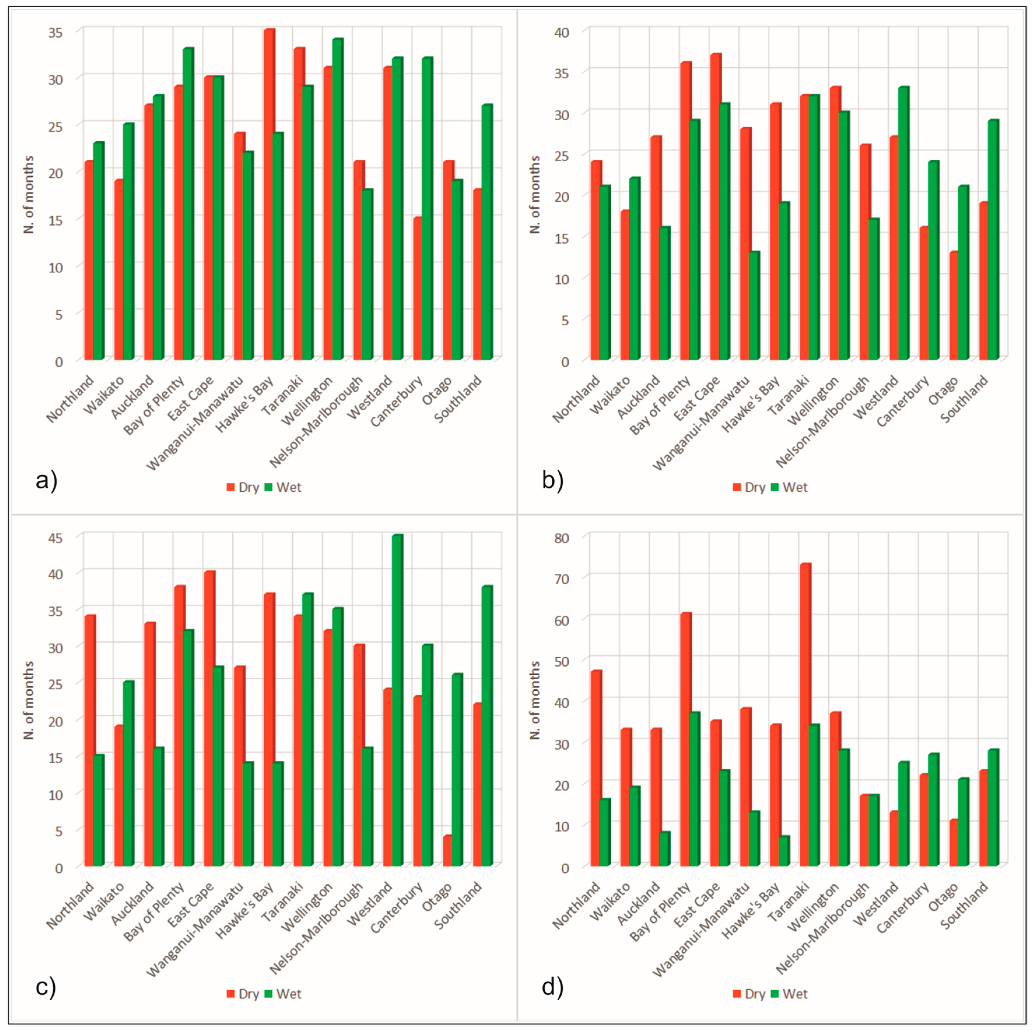
Before applying the ITA, the number of months showing severe or extreme dry and wet conditions was evaluated. As a result, different conditions have been detected considering the different time scales.
As to what concerns the 3-month SPI (Figure 3a) in nine out of 14 regions the number of months showing severe or extreme wet conditions is higher than the ones showing severe or extreme dry conditions. In particular, in the South Island, in the Canterbury and Southland areas, only in 15 and 18 months dry conditions have been detected while, instead, 32 and 27 months evidenced wet conditions, respectively. Differently from these regions, in the Hawke’s Bay area (North Island), the months that showed dry conditions (35 months) clearly outperform the months (24) in which wet conditions have been detected.
The 6-month SPI (Figure 3b) showed a different behavior with respect to the 3-month SPI. In fact, in eight regions, the number of months showing severe or extreme dry conditions is higher than the one presenting wet conditions. Dry conditions have been detected especially in the North Island and, specifically, in the Auckland (27 months against 16), Bay of Plenty (36 months against 29), East Cape (37 months against 31), Wanganui-Manawatu (28 months against 13), and Hawke’s Bay (31 months against 19) areas. In the South Island, only the Nelson-Marlborough region showed dry conditions in 26 months (17 wet months), while in the other regions, wet conditions have been evidenced.
Concerning the 12-month SPI (Figure 3c) an equal number of regions showed prevailing dry or wet conditions. In particular, in the North Island, in six out of nine regions, the number of months showing dry conditions is higher than the ones showing wet conditions. Conversely, in the South Island, four regions showed wet conditions, and only one region (Nelson-Marlborough) evidenced dry conditions. Specifically, in the North Island, relevant results have been obtained in the Bay of Plenty and in the East Cape regions, with 38 and 40 months showing severe or extreme dry conditions, respectively, while, in the South Island, the Westland (45 months against 24) and the Southland (38 months against 22) regions marked dry conditions have been detected.
Finally, the 24-month SPI (Figure 3d) showed a clear difference between the two islands. In fact, in the North Island, severe or extreme dry conditions have been detected in all the regions, while severe or extreme wet conditions have been detected in all the regions of the South Island. In particular, the driest conditions in the North Island have been detected in the Taranaki (73 months against 34) and in the Bay of Plenty (61 months against 37) regions, while, in the South Island, the Southland (73 months against 34) and the Canterbury (61 months against 37) areas showed the highest number of months with wet conditions.
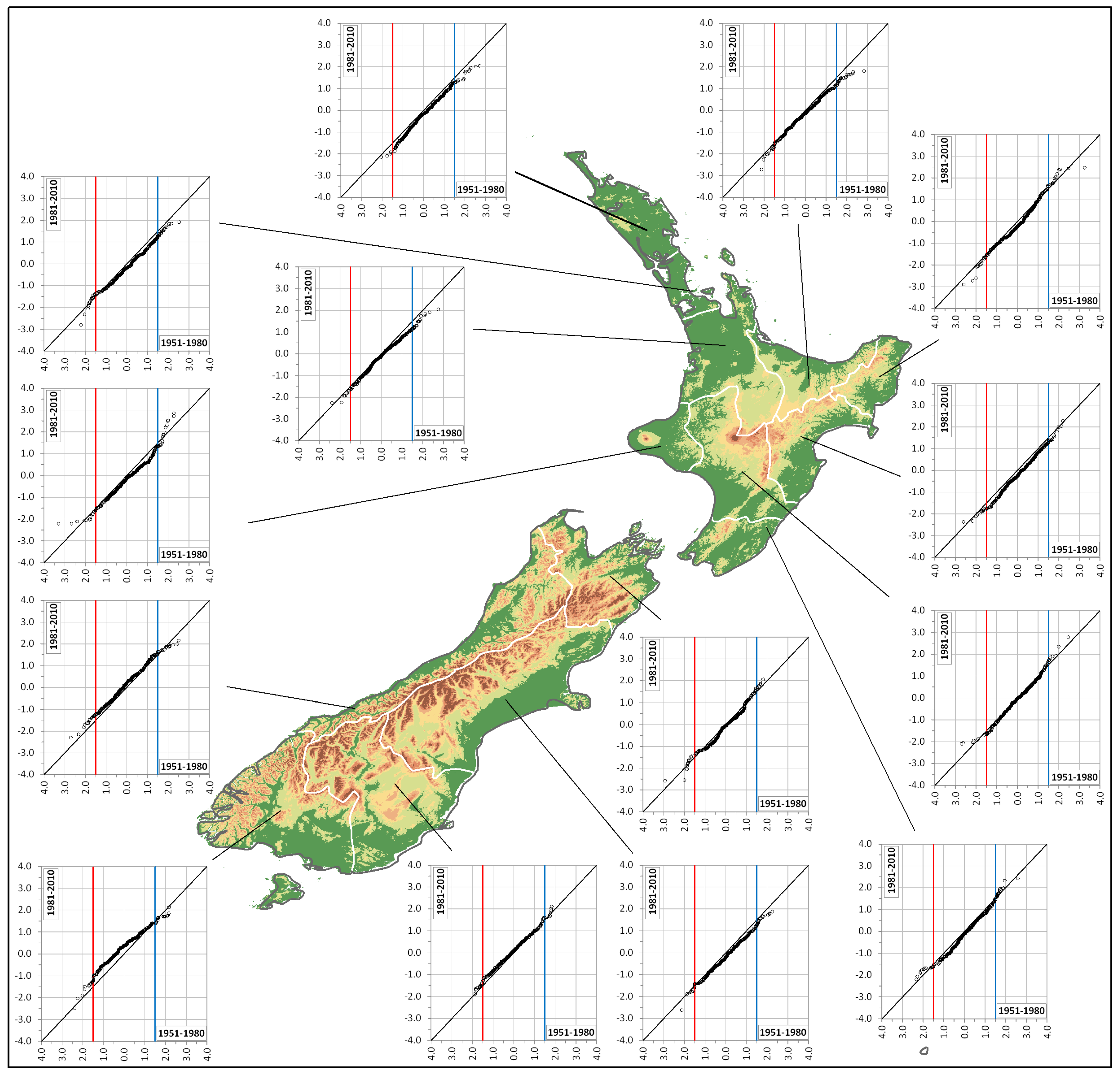
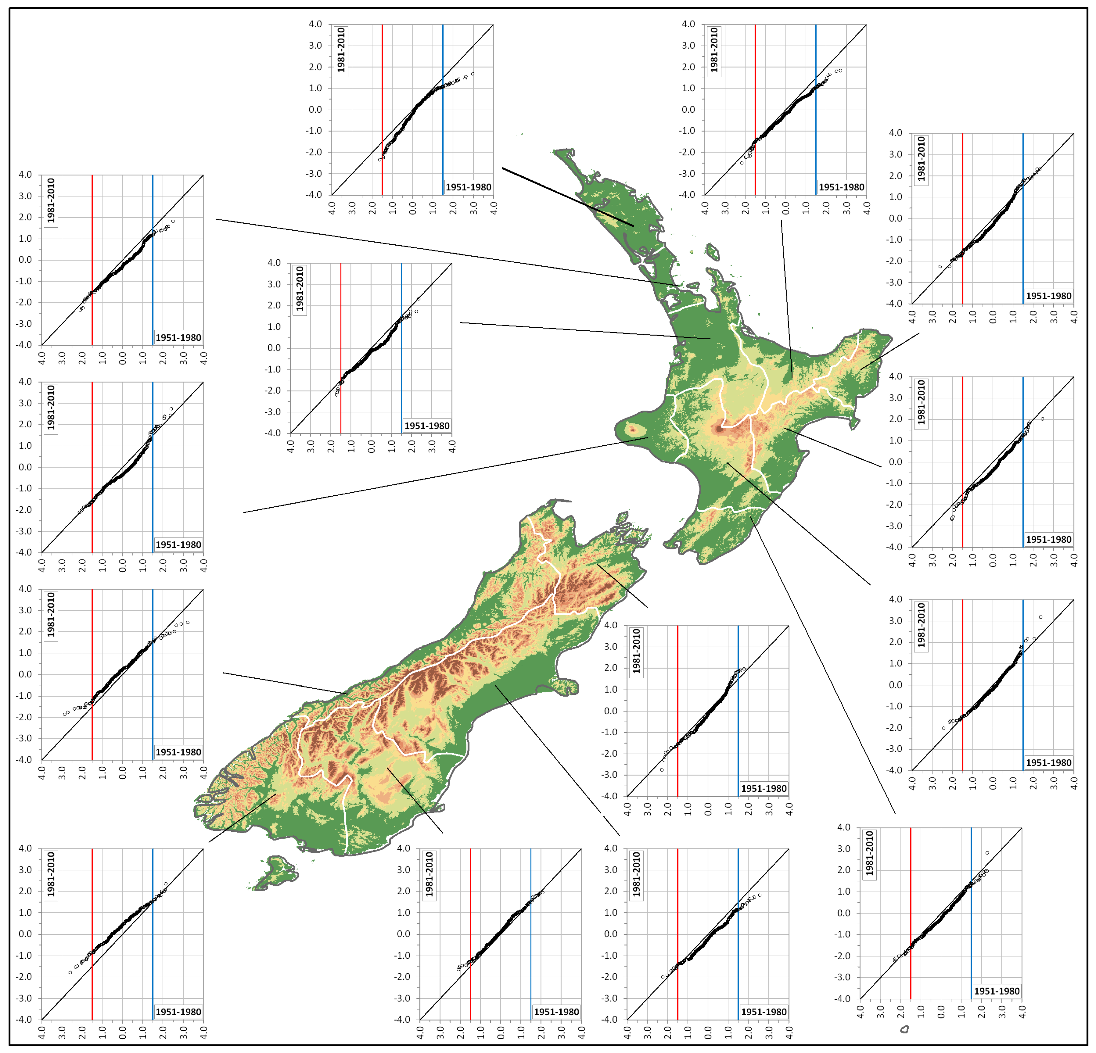
With the aim to detect possible trends in the 3-, 6-, 12-, and 24-month SPI values, for each region the ITA method was applied to the monthly series of the index. The ITA method allowed to evidence the tendencies of both low and high SPI values, thus including values referred to wet conditions. As a result of the ITA approach, Figure 4, Figure 5, Figure 6 and Figure 7 show the results obtained at regional level for the 3-, 6-, 12- and 24-month SPI, respectively. All the SPI series were divided into two 30-year sub-series: from 1951 to 1980, and from 1981 to 2010.
Generally, the main result obtained for the 3-month SPI values was a negative trend of the highest values of the index, which is related to weaker wet periods (Figure 4). This tendency has been detected in nine out of 14 regions but with a different behavior of the lowest SPI values. In fact, in four regions of the North Island (Northland, Auckland, Bay of Planty and East Cape) and in the Canterbury region in the South Island, a negative trend of both the lowest and the highest values of the index has been detected, thus evidencing heavier droughts and weaker wet periods. At the same time, in the Waikato, Wellington, Southland, and Westland regions, a positive trend of the lowest values and negative trend of the highest ones has been evidenced, both indicating weaker droughts and wet periods. Differently from the previous regions, the Otago, Wanganui-Manawatu, and Taranaki areas evidenced a tendency through weaker droughts and heavier wet periods given by a positive trend of both the lowest and the highest SPI values. Finally, in the Nelson-Marlborough region, a negative trend of the lowest values (heavier droughts) and a positive trend of the highest values (heavier wet periods) have been detected. The results of the ITA methods on the Hawke’s Bay region did not show a clear tendency, with the lowest and highest values falling close to the no trend line.
As regards the 6-month SPI, results confirm the ones obtained for the 3-month SPI, with a spreading negative trend of the highest values of the index (Figure 5). In fact, similar results to the 3-month SPI have been obtained in Northland, Auckland, Bay of Planty, Wanganui-Manawatu, Taranaki, Nelson-Marlborough, Westland, and Southland. Different from the results obtained for the 3-month SPI, in the Waikato and in the Hawke’s Bay regions, a negative trend of both the lowest and the highest values of the SPI index has been detected. Moreover, in the Canterbury and Otago region, a positive trend of the lowest values (weaker droughts) and a negative trend of the highest values (weaker wet periods) have been evidenced. Finally, the Wellington and East Cape regions did not show a clear tendency.
Studies on the 3- and 6-month SPI trends, which impact vegetation and agricultural practices, are paramount for New Zealand because agriculture is one of the largest sectors of the economy. As a summary of the results of the trend analysis on these time scales, in the South Island, which is generally characterized by wet conditions, a negative trend of the highest SPI value has been detected in the majority of the regions, thus indicating a tendency toward weaker wet periods. In particular, in the agricultural area of the Canterbury, the 3-month SPI evidenced a decreasing trend of both the lowest and the highest values of the index, which lead to heavier droughts and weaker wet periods. In the North Island, where the majority of the regions showed a higher percentage of dry months than wet months, a general negative trend of both the lowest and the highest SPI values has been identified, with the exception of some region such as Wanganui-Manawatu and Taranaki.
Considering the long time scales, the 12-month SPI trend showed similar results than the 6-month SPI but with an increase in the negative trend (Figure 6). In fact, in the Northland, Waikato, Auckland, Bay of Planty, East Cape, Hawke’s Bay, and Canterbury regions, a reduction of all the SPI values has been detected, thus confirming a clear tendency toward heavier droughts and weaker wet periods. On the contrary, the Wanganui-Manawatu, Nelson-Marlborough, and Otago regions showed trend results that indicate weaker droughts and heavier wet periods. An increase of the lowest values and a decrease in the highest values (weaker wet and dry periods) has been evidenced in the Wellington, Westland, and Southland regions. In the Taranaki area, no clear tendencies have been detected in the severe and extreme SPI values.
As regards the 24-month SPI, in eight regions (Northland, Waikato, Auckland, Bay of Planty, East Cape, Wanganui-Manawatu, Hawke’s Bay, and Canterbury), the results of the trend analysis with the ITA method evidenced a clear reduction of the lowest SPI values. Among these regions, the same result has been obtained for the highest values, with the exception of the Waikato and Auckland, in which the highest values showed a positive trend. By contrast, the Taranaki, Nelson-Marlborough, Otago Westland, and Southland regions showed an increase in the lowest values, with concomitant decrease in the highest values in the Taranaki and Otago areas and increase in the highest values in the Nelson-Marlborough, Westland, and Southland regions. As also evidenced for the 3-month SPI, the Wellington region did not show a clear tendency.
The 12- and 24-month SPI are a broad proxy for water resource management. Results of the trend analysis on these time scales confirm the ones obtained on a short time scale but with an increase in the number of regions where a negative trend has been detected. In fact, current global level assessments suggest that droughts are expected to both increase and decrease following future climate change depending upon geographic location [66]. Based on the latest climate and impact modelling, New Zealand can expect more droughts in the future in some locations [51].
As a result, this work has evidenced an increase in drought trend in all the areas that are presently subject to drought, supporting what has been evidenced in past studies [50,64]. In fact, the results of this paper confirm the geographic pattern of change found by Mullan et al. [50] and Caloiero [64], which mainly detected a drought increase in the future projections on the East Coast and no change in drought projections for the West Coast of the South Island. Specifically, as also evidenced by Clark et al. [51] and Caloiero [64], the results of this paper highlight that key agricultural regions on the Eastern side such as the Canterbury Plains are the most consistently vulnerable areas in the South Island, together with other regions in the North Island, including a key primary industry region like Waikato.
5. Conclusions
Generally, the methods used for trend detection allow researchers to analyze general tendencies of climatic variables, but they do not make it possible to identify sub-trends. In this paper, for every region of New Zealand, an average SPI series has first been evaluated at various time scales (3, 6, 12, and 24 months). Then, for each region, the number of months showing severe or extreme dry and wet conditions has been detected. Finally, a graphical technique, based on the Innovative Trend Analysis (ITA) proposed by Şen [39], was applied to the SPI series. As a result, a different behavior emerged between the two islands. In fact, for the several time scale, in the majority of the regions of the North Island, the number of months showing dry conditions is higher than the ones showing wet conditions, while in the South Island, the number of months showing wet conditions is higher than the ones showing dry conditions. In particular, for the 24-month time scale, dry conditions have been detected in all the regions of the North Island, while wet conditions have been detected in the South Island ones. As to what concerns the trend analysis, on a short time scale, the results showed a negative trend of the highest SPI value in the South Island, thus indicating a tendency toward weaker wet periods. In particular, in the agricultural area of the Canterbury, the 3-month SPI evidenced a decreasing trend in both the lowest and the highest values of the index, which lead to heavier droughts and weaker wet periods. In the North Island, a general negative trend of both the lowest and the highest SPI values has been identified, thus evidencing heavier droughts and weaker wet periods. Results of the trend analysis on long time scales confirm the ones obtained on a short time scale but with an increase in the number of regions where a negative trend has been detected, highlighting that agricultural regions on the eastern side of the South Island, as well as the north-eastern regions of the North Island, are the most consistently vulnerable areas.
Acknowledgments
The author would like to thank the National Institute of Water and Atmosphere Research for providing access to the New Zealand meteorological data from the National Climate Database.
Conflicts of Interest
The author declares no conflict of interest.
References
- Estrela, T.; Vargas, E. Drought management plans in the European Union. Water Resour. Manag. 2010, 26, 1537–1553. [Google Scholar] [CrossRef]
- Kreibich, H.; Di Baldassarre, G.; Vorogushyn, S.; Aerts, J.C.J.H.; Apel, H.; Aronica, G.T.; Arnbjerg-Nielsen, K.; Bouwer, L.M.; Bubeck, P.; Caloiero, T.; et al. Adaptation to flood risk: Results of international paired flood event studies. Earth’s Future 2017, 5, 953–965. [Google Scholar] [CrossRef]
- Wilhite, D.A.; Hayes, M.J.; Svodoba, M.D. Drought monitoring and assessment in the US. In Drought and Drought Mitigation in Europe; Voght, J.V., Somma, F., Eds.; Kluwers: Dordrecht, The Netherlands, 2000; pp. 149–160. [Google Scholar]
- Yevjevich, V.; Da Cunha, L.; Vlachos, E. Coping with Droughts; Water Resources Publications: Littleton, CO, USA, 1983. [Google Scholar]
- Fink, A.H.; Brücher, T.; Krüger, A.; Leckebush, G.C.; Pinto, J.G.; Ulbrich, U. The 2003 European summer heatwaves and drought-synoptic diagnosis and impacts. Weather 2004, 59, 209–216. [Google Scholar] [CrossRef] [Green Version]
- Lloyd-Huhes, B.; Saunders, M.A. A drought climatology for Europe. Int. J. Climatol. 2002, 22, 1571–1592. [Google Scholar] [CrossRef]
- Zaidman, M.D.; Rees, H.G.; Young, A.R. Spatio-temporal development of streamflow droughts in north-west Europe. Hydrol. Earth Syst. Sci. 2012, 5, 733–751. [Google Scholar] [CrossRef]
- Hannaford, J.; Lloyd-Hughes, B.; Keef, C.; Parry, S.; Prudhomme, C. Examining the large-scale spatial coherence of European drought using regional indicators of precipitation and streamflow deficit. Hydrol. Process. 2011, 25, 1146–1162. [Google Scholar] [CrossRef]
- Intergovernmental Panel on Climate Change (IPCC). Summary for Policymakers; Fifth Assessment Report of the Intergovernmental Panel on Climate Change; Cambridge University Press: Cambridge, UK, 2013. [Google Scholar]
- Buttafuoco, G.; Caloiero, T.; Ricca, N.; Guagliardi, I. Assessment of drought and its uncertainty in a southern Italy area (Calabria region). Measurement 2018, 113, 205–210. [Google Scholar] [CrossRef]
- Caloiero, T.; Coscarelli, R.; Ferrari, E.; Sirangelo, B. Analysis of Dry Spells in Southern Italy (Calabria). Water 2015, 7, 3009–3023. [Google Scholar] [CrossRef]
- Fang, K.; Gou, X.; Chen, F.; Davi, N.; Liu, C. Spatiotemporal drought variability for central and eastern Asia over the past seven centuries derived from tree-ring based reconstructions. Quat. Int. 2013, 283, 107–116. [Google Scholar] [CrossRef]
- Feng, S.; Hu, Q.; Oglesby, R.J. Influence of Atlantic sea surface temperatures on persistent drought in North America. Clim. Dyn. 2011, 37, 569–586. [Google Scholar] [CrossRef]
- Hua, T.; Wang, X.M.; Zhang, C.X.; Lang, L.L. Temporal and spatial variations in the Palmer Drought Severity Index over the past four centuries in arid, semiarid, and semihumid East Asia. Chin. Sci. Bull. 2013, 58, 4143–4152. [Google Scholar] [CrossRef]
- Minetti, J.L.; Vargas, W.M.; Poblete, A.G.; de la Zerda, L.R.; Acuña, L.R. Regional droughts in southern South America. Theor. Appl. Climatol. 2010, 102, 403–415. [Google Scholar] [CrossRef]
- Sirangelo, B.; Caloiero, T.; Coscarelli, R.; Ferrari, E. A stochastic model for the analysis of the temporal change of dry spells. Stoch. Environ. Res. Risk Assess. 2015, 29, 143–155. [Google Scholar] [CrossRef]
- Sirangelo, B.; Caloiero, T.; Coscarelli, R.; Ferrari, E. Stochastic analysis of long dry spells in Calabria (Southern Italy). Theor. Appl. Climatol. 2017, 127, 711–724. [Google Scholar] [CrossRef]
- Tsakiris, G.; Pangalou, D.; Vangelis, H. Regional drought assessment based on the Reconnaissance Drought Index (RDI). Water Resour. Manag. 2007, 21, 821–833. [Google Scholar] [CrossRef]
- Tabari, H.; Abghari, H.; Hosseinzadeh Talaee, P. Temporal trends and spatial characteristics of drought and rainfall in arid and semi-arid regions of Iran. Hydrol. Process. 2012, 26, 3351–3361. [Google Scholar] [CrossRef]
- Bayissa, Y.A.; Moges, S.A.; Xuan, Y.; Van Andel, S.J.; Maskey, S.; Solomatine, D.P.; Griensven, A.; Van Tadesse, T. Spatio-temporal assessment of meteorological drought under the influence of varying record length: The case of Upper Blue Nile Basin, Ethiopia. Hydrol. Sci. J. 2015, 60, 1927–1942. [Google Scholar] [CrossRef]
- McKee, T.B.; Doesken, N.J.; Kleist, J. The relationship of drought frequency and duration to time scales. In Proceedings of the 8th Conference on Applied Climatology, Anaheim, CA, USA, 17–22 January 1993; pp. 179–184. [Google Scholar]
- Khan, S.; Gabriel, H.F.; Rana, T. Standard precipitation index to track drought and assess impact of rainfall on watertables in irrigation areas. Irrig. Drain. Syst. 2008, 22, 159–177. [Google Scholar] [CrossRef]
- Logan, K.E.; Brunsell, N.A.; Jones, A.R.; Feddema, J.J. Assessing spatiotemporal variability of drought in the US central plains. J. Arid Environ. 2010, 74, 247–255. [Google Scholar] [CrossRef]
- Manatsa, D.; Mukwada, G.; Siziba, E.; Chinyanganya, T. Analysis of multidimensional aspects of agricultural droughts in Zimbabwe using the Standardized Precipitation Index (SPI). Theor. Appl. Climatol. 2010, 102, 287–305. [Google Scholar] [CrossRef]
- Patel, N.R.; Yadav, K. Monitoring spatio-temporal pattern of drought stress using integrated drought index over Bundelkhand region, India. Nat. Hazards 2015, 77, 663–677. [Google Scholar] [CrossRef]
- Raziei, T.; Saghafian, B.; Paulo, A.A.; Pereira, L.S.; Bordi, I. Spatial patterns and temporal variability of drought in Western Iran. Water Resour. Manag. 2009, 23, 439–455. [Google Scholar] [CrossRef]
- Buttafuoco, G.; Caloiero, T. Drought events at different timescales in southern Italy (Calabria). J. Maps 2014, 10, 529–537. [Google Scholar] [CrossRef]
- Zhai, L.; Feng, Q. Spatial and temporal pattern of precipitation and drought in Gansu Province Northwest China. Nat. Hazards 2009, 49, 1–24. [Google Scholar] [CrossRef]
- Capra, A.; Scicolone, B. Spatiotemporal variability of drought on a short–medium time scale in the Calabria Region (Southern Italy). Theor. Appl. Climatol. 2012, 3, 471–488. [Google Scholar] [CrossRef]
- Wu, H.; Hayes, M.J.; Wilhite, D.A.; Svoboda, M.D. The effect of the length of record on the standardized precipitation index calculation. Int. J. Climatol. 2005, 25, 505–520. [Google Scholar] [CrossRef]
- Vicente-Serrano, S.M. Differences in spatial patterns of drought on different time sales: An analysis of the Iberian Peninsula. Water Resour. Manag. 2006, 20, 37–60. [Google Scholar] [CrossRef]
- Buttafuoco, G.; Caloiero, T.; Coscarelli, R. Analyses of Drought Events in Calabria (Southern Italy) Using Standardized Precipitation Index. Water Resour. Manag. 2015, 29, 557–573. [Google Scholar] [CrossRef]
- Caloiero, T.; Coscarelli, R.; Ferrari, E.; Sirangelo, B. An Analysis of the Occurrence Probabilities of Wet and Dry Periods through a Stochastic Monthly Rainfall Model. Water 2016, 8, 39. [Google Scholar] [CrossRef]
- Guttman, N.B. Accepting the standardized precipitation index: A calculating algorithm. J. Am. Water Resour. Assoc. 1999, 35, 311–323. [Google Scholar] [CrossRef]
- Cancelliere, A.; Di Mauro, G.; Bonaccorso, B.; Rossi, G. Drought forecasting using the Standardised Precipitation Index. Water Resour. Manag. 2007, 21, 801–819. [Google Scholar] [CrossRef]
- Bordi, I.; Fraedrich, K.; Sutera, A. Observed drought and wetness trends in Europe: An update. Hydrol. Earth Syst. Sci. 2009, 13, 1519–1530. [Google Scholar] [CrossRef]
- Golian, S.; Mazdiyasni, O.; AghaKouchak, A. Trends in meteorological and agricultural droughts in Iran. Theor. Appl. Climatol. 2015, 119, 679–688. [Google Scholar] [CrossRef]
- Zhai, J.; Su, B.; Krysanova, V.; Vetter, T.; Gao, C.; Jiang, T. Spatial variation and trends in PDSI and SPI indices and their relation to streamflow in 10 large regions of China. J. Clim. 2010, 23, 649–663. [Google Scholar] [CrossRef]
- Şen, Z. An innovative trend analysis methodology. J. Hydrol. Eng. 2012, 17, 1042–1046. [Google Scholar] [CrossRef]
- Haktanir, T.; Citakoglu, H. Trend, independence, stationarity, and homogeneity tests on maximum rainfall series of standard durations recorded in Turkey. J. Hydrol. Eng. 2014, 19, 501–509. [Google Scholar] [CrossRef]
- Kisi, O.; Ay, M. Comparison of Mann–Kendall and innovative trend method for water quality parameters of the Kizilirmak River, Turkey. J. Hydrol. 2014, 513, 362–375. [Google Scholar] [CrossRef]
- Şen, Z. Trend identification simulation and application. J. Hydrol. Eng. 2014, 19, 635–642. [Google Scholar] [CrossRef]
- Ay, M.; Kisi, O. Investigation of trend analysis of monthly total precipitation by an innovative method. Theor. Appl. Climatol. 2015, 120, 617–629. [Google Scholar] [CrossRef]
- Martínez-Austria, P.F.; Bandala, E.R.; Patiño-Gómez, C. Temperature and heat wave trends in northwest Mexico. Phys. Chem. Earth 2015, 91, 20–26. [Google Scholar] [CrossRef]
- Kisi, O. An innovative method for trend analysis of monthly pan evaporations. J. Hydrol. 2015, 527, 1123–1129. [Google Scholar] [CrossRef]
- Tabari, H.; Willems, P. Investigation of streamflow variation using an innovative trend analysis approach in northwest Iran. In Proceedings of the 36th IAHR World Congress, The Hague, The Nederland, 28 June–3 July 2015. [Google Scholar]
- Palmer, J.G.; Cook, E.R.; Turney, C.S.M.; Allen, K.; Fenwick, P.; Cook, B.; O’Donnell, A.J.; Lough, J.M.; Grierson, P.F.G.; Baker, P. Drought variability in the eastern Australia and New Zealand summer drought atlas (ANZDA, CE 1500–2012) modulated by the Interdecadal Pacific Oscillation. Environ. Res. Lett. 2015, 10, 124002. [Google Scholar] [CrossRef]
- MAF. Regional and National Impacts of the 2007–2008 Drought; Butcher Partners Ltd.: Tai Tapu, New Zealand, 2009. [Google Scholar]
- Kamber, G.; McDonald, C.; Price, G. Drying Out: Investigating the Economic Effects of Drought in New Zealand; Reserve Bank of New Zealand: Wellington, New Zealand, 2013. [Google Scholar]
- Mullan, B.; Porteous, A.; Wratt, D.; Hollis, M. Changes in Drought Risk with Climate Change; National Institute of Water & Atmospheric Research: Wellington, New Zealand, 2015. [Google Scholar]
- Clark, A.; Mullan, B.; Porteous, A. Scenarios of Regional Drought under Climate Change; National Institute of Water & Atmospheric Research: Wellington, New Zealand, 2011. [Google Scholar]
- Edwards, D.; McKee, T. Characteristics of 20th Century Drought in the United States at Multiple Scale; Atmospheric Science Paper 634; Department of Atmospheric Science Colorado State University: Fort Collins, CO, USA, 1997. [Google Scholar]
- Bonaccorso, B.; Bordi, I.; Cancelliere, A.; Rossi, G.; Sutera, A. Spatial variability of drought: An analysis of SPI in Sicily. Water Resour. Manag. 2003, 17, 273–296. [Google Scholar] [CrossRef]
- Angelidis, P.; Maris, F.; Kotsovinos, N.; Hrissanthou, V. Computation of drought index SPI with Alternative Distribution Functions. Water Resour. Manag. 2012, 26, 2453–2473. [Google Scholar] [CrossRef]
- Thom, H.C.S. A note on the gamma distribution. Mon. Weather Rev. 1958, 86, 117–122. [Google Scholar] [CrossRef]
- Abramowitz, M.; Stegun, I.A. Handbook of Mathematical Functions with Formulas, Graphs, and Mathematical Tables; Dover Publications, INC.: New York, NY, USA, 1970. [Google Scholar]
- Oliver, J.E. Encyclopedia of World Climatology; Springer: Amsterdam, The Netherlands, 2005. [Google Scholar]
- NIWA. Overview of New Zealand Climate. Available online: http://www.niwa.co.nz/education-and-training/schools/resources/climate/overview (accessed on 26 February 2018).
- Salinger, M.J.; Mullan, A.B. New Zealand climate: Temperature and precipitation variations and their links with atmospheric circulation 1930–1994. Int. J. Climatol. 1999, 19, 1049–1071. [Google Scholar] [CrossRef]
- Griffiths, G.M.; Salinger, M.J.; Leleu, I. Trends in extreme daily rainfall across the South Pacific and relationship to the South Pacific Convergence Zone. Int. J. Climatol. 2003, 23, 847–869. [Google Scholar] [CrossRef]
- Dravitzki, S.; McGregor, J. Extreme precipitation of the Waikato region, New Zealand. Int. J. Climatol. 2011, 31, 1803–1812. [Google Scholar] [CrossRef]
- Caloiero, T. Analysis of daily rainfall concentration in New Zealand. Nat. Hazards 2014, 72, 389–404. [Google Scholar] [CrossRef]
- Caloiero, T. Analysis of rainfall trend in New Zealand. Environ. Earth. Sci. 2015, 73, 6297–6310. [Google Scholar] [CrossRef]
- Caloiero, T. Drought analysis in New Zealand using the standardized precipitation index. Environ. Earth. Sci. 2017, 76, 569. [Google Scholar] [CrossRef]
- Caloiero, T. Trend of monthly temperature and daily extreme temperature during 1951–2012 in New Zealand. Theor. Appl. Climatol. 2017, 129, 111–117. [Google Scholar] [CrossRef]
- Wang, G. Agricultural drought in a future climate: Results from 15 global climate models participating in the IPCC 4th assessment. Clim. Dyn. 2005, 25, 739–753. [Google Scholar] [CrossRef]
Figure 1.
Example of the Innovative Trend Analysis (ITA) proposed by Şen [39].
Figure 1.
Example of the Innovative Trend Analysis (ITA) proposed by Şen [39].
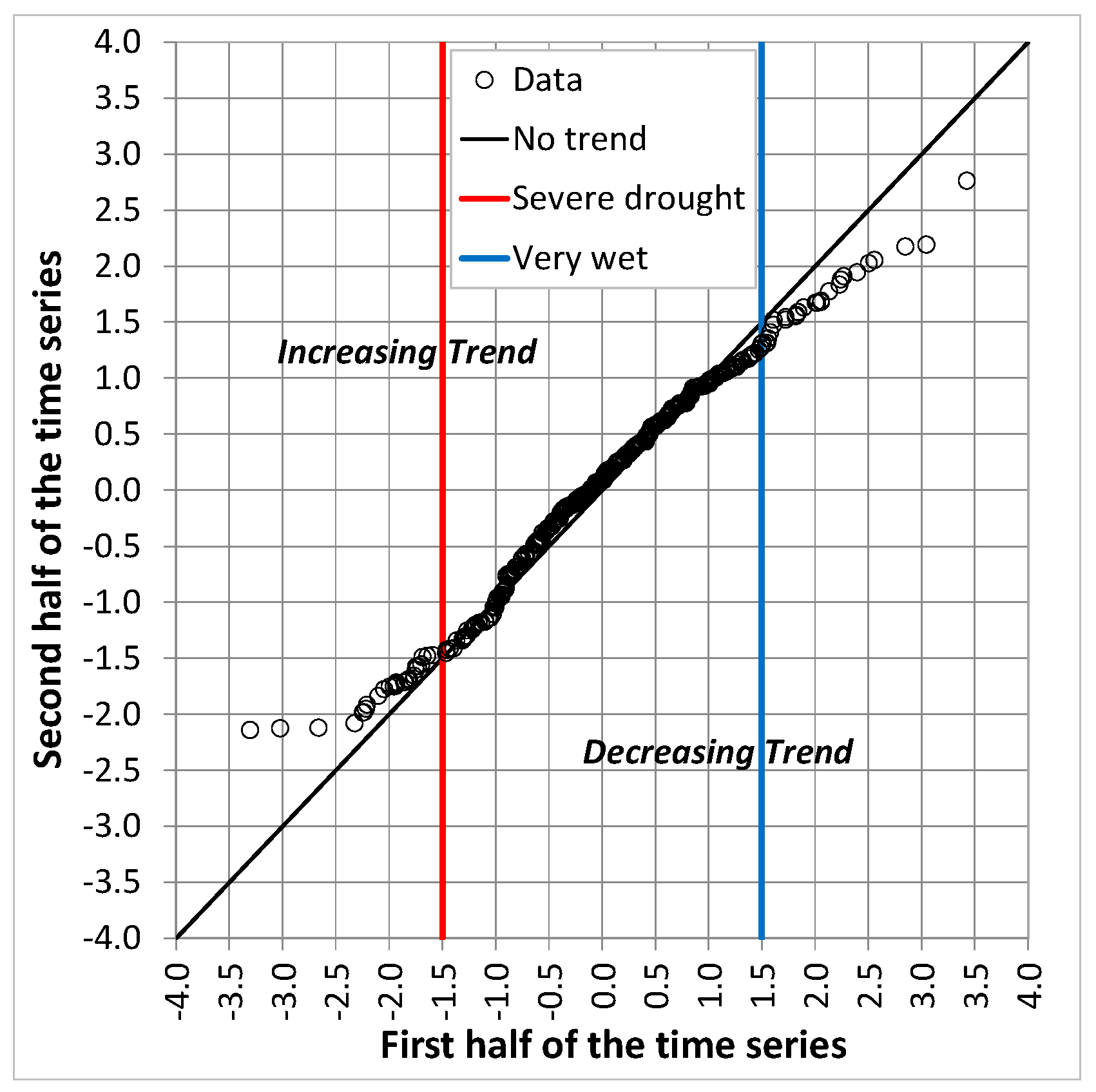
Figure 2.
Location of the 14 regions of New Zealand and of the selected 294 rain gauge stations on a Digital Elevation Model (DEM) of New Zealand.
Figure 2.
Location of the 14 regions of New Zealand and of the selected 294 rain gauge stations on a Digital Elevation Model (DEM) of New Zealand.
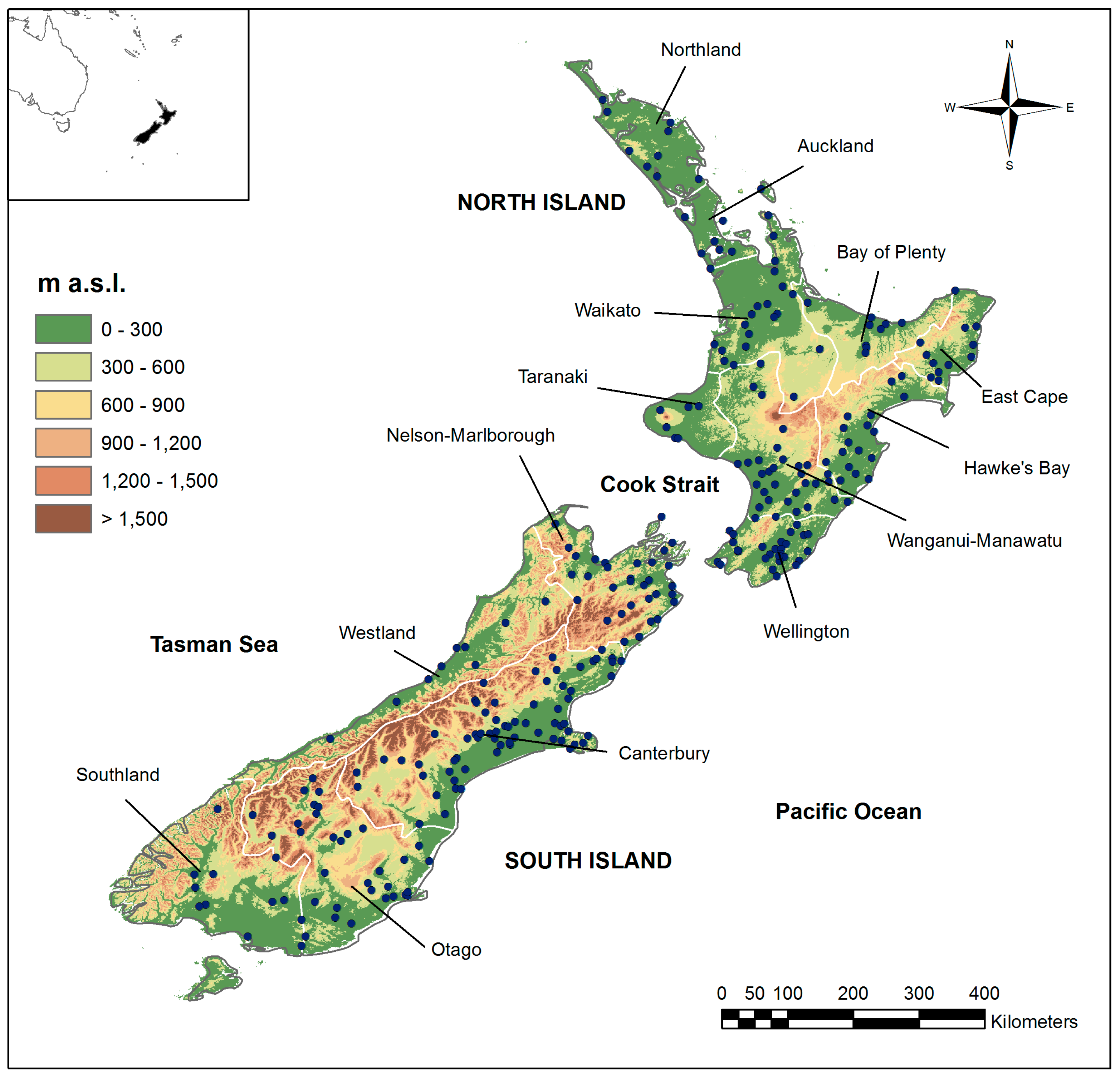
Figure 3.
Number of months showing severe or extreme dry and wet conditions for the 3-month (a); 6-month (b); 12-month (c); and 24-month SPI (d).
Figure 3.
Number of months showing severe or extreme dry and wet conditions for the 3-month (a); 6-month (b); 12-month (c); and 24-month SPI (d).

Figure 4.
Regional results of the Innovative Trend Analysis (ITA) method applied to the 3-month SPI.
Figure 4.
Regional results of the Innovative Trend Analysis (ITA) method applied to the 3-month SPI.

Figure 5.
Regional results of the ITA method applied to the 6-month SPI.

Figure 6.
Regional results of the ITA method applied to the 12-month SPI.

Figure 7.
Regional results of the ITA method applied to the 24-month SPI.


Table 1.
Climate classification according to the Standardized Precipitation Index (SPI) values.
| SPI Value | Class | Probability (%) |
|---|---|---|
| SPI ≥ 2.00 | Extremely wet | 2.3 |
| 1.5 ≤ SPI < 2.00 | Severely wet | 4.4 |
| SPI < 1.50 | Moderately wet | 9.2 |
| SPI < 1.00 | Mildly wet | 34.1 |
| −1.00 ≤ SPI < 0.00 | Mild drought | 34.1 |
| −1.50 ≤ SPI < −1.00 | Moderate drought | 9.2 |
| −2.00 ≤ SPI < −1.50 | Severe drought | 4.4 |
| SPI < −2.00 | Extreme drought | 2.3 |
© 2018 by the author. Licensee MDPI, Basel, Switzerland. This article is an open access article distributed under the terms and conditions of the Creative Commons Attribution (CC BY) license (http://creativecommons.org/licenses/by/4.0/).
Share and Cite
MDPI and ACS Style
Caloiero, T. SPI Trend Analysis of New Zealand Applying the ITA Technique. Geosciences 2018, 8, 101. https://doi.org/10.3390/geosciences8030101
AMA Style
Caloiero T. SPI Trend Analysis of New Zealand Applying the ITA Technique. Geosciences. 2018; 8(3):101. https://doi.org/10.3390/geosciences8030101
Chicago/Turabian StyleCaloiero, Tommaso. 2018. "SPI Trend Analysis of New Zealand Applying the ITA Technique" Geosciences 8, no. 3: 101. https://doi.org/10.3390/geosciences8030101
Note that from the first issue of 2016, this journal uses article numbers instead of page numbers. See further details here.