Repetitive Rockfall Trajectory Testing
by
Axel Volkwein
1,*, 
Lucas Brügger
2,
Fabio Gees
2,
Werner Gerber
1,
Barbara Krummenacher
1,†,
Peter Kummer
1,
Jessica Lardon
2 and
Tobias Sutter
2 1
WSL Swiss Federal Institute for Forest, Snow and Landscape Research, 8903 Birmensdorf, Switzerland
2
Zurich University of Applied Sciences/ZHAW, Life Sciences und Facility Management, 8820 Wädenswil, Switzerland
*
Author to whom correspondence should be addressed.
†
Current address: University of Applied Sciences HTW Chur, 7004 Chur, Switzerland.
Geosciences 2018, 8(3), 88; https://doi.org/10.3390/geosciences8030088
Submission received: 9 January 2018
/
Revised: 8 February 2018
/
Accepted: 24 February 2018
/
Published: 7 March 2018
Abstract
:Numerical simulations of rockfall trajectories are a standard procedure for evaluating rockfall hazards. For these simulations, corresponding software codes must be calibrated and evaluated based on field data. This study addresses methods of repeatable rockfall tests, and investigates whether it is possible to produce traceable and statistically analysable data. A testing series is described extensively covering how to conduct rockfall experiments and how certain elements of rockfall trajectories can be measured. The tests use acceleration and rotation sensors inside test blocks, a system to determine block positions over time, surveying measurements, and video recordings. All systems are evaluated regarding their usability in the field and for analyses. The highly detailed description of testing methods is the basis for sound understanding and reproducibility of the tests. This article serves as a reference for future publications and other rockfall field tests, both as a guide and as a basis for comparisons. First analyses deliver information on runout with a shadow angle ranging between 21 and 45 degrees for a slope consisting of homogeneous soft soil. A digital elevation model of the test site as well as point clouds of the used test blocks are part of this publication.
1. Introduction
Rockfall trajectory simulation software can deliver information on velocities and runout distances. The corresponding numerical models must be calibrated based on field data. Such field data can be obtained through the posterior analysis of natural rockfall events. The trajectory is then determined based on traces in the field during impacts, the starting and the final position of a block. Gerber [1] describes how maximum velocities and individual jump heights of the block’s trajectory can be derived. The block shape and size can be determined at the final position and the mass can be estimated based on this. However, as the analysed event is usually only a random sample of many different possible rockfalls there is no information as to whether the recorded rockfall is an average or an extreme event. A probabilistic analysis as for example described in Ferrari et al. [2] is therefore necessary.
Data necessary for the calibration of a rock trajectory simulation code can also be gathered through carrying out special rockfall experiments. In this case, several blocks are released from the top of a rockfall slope. The repetition of this procedure delivers further knowledge of the possible variety of single rockfalls along this slope.
This article describes conducted field tests, which act as a guide and reference for further publications. The detailed description of the tests should furthermore allow the comparison of these tests with similar field tests. We hope that a large database will develop over time, including results from tests using a variety of different blocks and—more importantly—on different slopes. The data obtained would then allow better calibration of trajectory simulation codes.
After a short review of previously described tests with respect to better trajectory modelling, the article goes on to describe the current site and the test setup in detail. After describing the conducted tests summary results are presented. Section 4 shows example results that were received from the different measurement systems. The measurements are then evaluated. The article finishes with concluding remarks on the knowledge gained during the test series. The conclusion critically reviews the test setup.
1.1. Previous Rockfall Testing Series
Giani et al. [3,4] reported several rockfall tests in Italy in the early millennium to derive the trajectories and focus especially on coefficients of restitution for block impact.
Several hundred blocks were released at both forested and non-forested test sites in Vaujany, France by Dorren et al. [5]. Video analysis of the tests delivered valuable data on the height and velocity of block jumps, and the interaction between blocks and trees allowed the calibration of a numerical protection forest. If not blocked by an obstacle along the slope, the blocks usually came to a stop in the river at the bottom of the valley. Therefore, the maximum runout was pre-defined.
Preh et al. [6] positioned several hundred blocks on top of a cliff within a quarry to study the impact on a flat surface below, and the reach of the runout. These tests were performed to establish safety guidelines for the quarry regarding the risk of rockfall both for people and machines. The laboratory-like setup enabled extensive statistical analysis regarding impact and rebound velocities, energy lines, rotational effects and coefficients of restitution. The measurement methods consisted mainly of recordings of the blocks starting and final positions, marks on the ground, and video recordings provided additional information on trajectory kinetics. Such analyses are also described in Gerber [7].
1.2. Laboratory Rockfall Testing
One main factor for modelling rockfall trajectories is ideal mapping of the interaction between an impacting block and the surface underneath. Often this interaction is described using two different coefficients of restitution, one normal and one parallel to the slope. Laboratory tests provide an efficient method to produce recommendations for these values. Half-scale impact experiments on soil are for example described by Labiouse et al. [8] and Labiouse & Heidenreich [9].
Glover [10] used laboratory tests to study the influence of the rock-shape on runout and lateral deviation, using a setup with differently but regularly shaped aluminium blocks impacting an inclined wooden slope.
Rockfall tests (carried out under strictly controlled field conditions) describing the interaction between impacting blocks and the ground regarding the deceleration of the block itself and its penetration of the ground exist within the literature. The tests of Gerber & Volkwein [11] and Lambert et al. [12] were originally performed for the design of embankments. However, such measurements also help to improve the simulation of rockfalls in the field.
2. Field Test Preparation
The field tests described in this article were novel. Prior knowledge was available from a testing series described by Volkwein and Klette [13] where some of the measurement techniques of Section 2.5 were described. The current section first describes the boundary conditions for the tests, the chosen test setup consisting of test blocks, test site, their preparation and the measurement systems used.
2.1. Boundary Conditions
The aim of this field testing series was primarily to study the possibility of conducting rockfall field experiments with numerous different measurements, which would provide sufficient data for the extensive analysis of single trajectories. Due to financial limitation it was not possible to establish a test setup with large rock blocks as their handling would require heavy equipment.
The main idea was to throw numerous natural rock blocks down a natural hill/slope in order to gather information on the natural runout of the blocks. This required a slope with sections of varying inclination, steep enough in the first section to accelerate the moving blocks and flat enough in the final section to enable a natural runout until the complete stop of the blocks. The size of the testing area should not extend above 200 m × 100 m in order to use the local positioning system described in Section 2.5 and to still be able to film the rockfall process down the slope.
Ideally, the slope is not completely straight, but it reflects a typical full-size natural slope in its topography with channels, bumps, changing lateral inclination etc.; otherwise only the block shapes would influence the trajectories. Furthermore, we were interested in a rather homogeneous surface structure. For the calibration of rockfall simulation software there are many parameters that influence a simulation result. Therefore, the number of unknown parameters is reduced when the ground parameters do not vary greatly.
The most important aspect to consider in the test set-up was that we wanted to re-use the thrown blocks for several reasons. The main reason is that only through re-using the blocks it is possible to evaluate the repeatability of rockfall tests, i.e., the sensitivity of a single rockfall regarding small changes in topography, release conditions, etc. As described above, the restricted resources allowed more tests if the number of different blocks used was not too high. Further, we planned to install sensors within the testing blocks. This required prior preparation of the blocks with boreholes. Finally, using the testing slope required the removal of the thrown blocks post-testing, as such the blocks had to be transportable.
The re-use of the test blocks required good accessibility to both the test slope at the release region and the complete runout zone to transport the blocks. The transport of the blocks depended on their weight. Small blocks can manually be lifted onto a transport vehicle or manually being carried for short distances. Larger blocks however would require a mechanical device for their pick-up and transportation.
Ideally, the blocks hold their shape for repeated testing and do not suffer damage from individual rockfall tests.
2.2. Test Site Description
The test site is located down-hill of the “Oberalp” pass, close to the village of Tschamut in the Swiss Canton Grisons (Figure 1a). The rockfalls were released between the WGS84-positions N4639.227 E842.050 and N4639.242 E842.087 (in CH-1903 coordinates 696613.9/167726.6 to 696,659.9/167,755.8) at heights between 1676.3 and 1870.2 m a.s.l. (see Table 1 for coordinates of single start positions). The blocks were placed on the edge of the road and then pushed over. Initially they free fall past a road supporting wall (see Figure 2a) and then hit a small gravel bench. From there the individual trajectories travelled in the direction SSE, up to ca. 130 m horizontally and 50 m vertically. The testing area covers an (horizontally projected) area of about 9000 m. The slope is steeper in the upper part with an inclination ranging between and . At 1633–1637 m a.s.l. there is a clear transition to a less steep slope (inclination ca. ), followed by an almost horizontal runout zone with an inclination less than down to m a.s.l. These different zones are marked in Figure 1. The topography is mainly defined through a small depression in the right half and two terraces in the left half of the slope. These topographic elements are also visible for six exemplary slope profiles in Figure 2d.
The surface within the testing area is almost completely covered by grass. In some steep parts the bedrock is exposed (Figure 2a,b), in all other areas the bedrock is covered by shallow soil. The steeper area is usually used in the summer as pasture, whereas the lower parts are cut for hay/silage production. The ground is therefore classed as very soft. To quantify the ground characteristics the testing area was probed using a light weight deflectometer. Weber [14] delivered ME values ranging from 3 ± 2 MN/m in the steeper area to 4 ± 2 MN/m in the flat runout area. In the previously mentioned depression there are some bushes (Figure 1b). A small swamp-like area is also marked in Figure 1b.
Test sites which fulfil the conditions described in Section 2.1 are often found in cultivated areas. In our case, several actions were necessary prior to testing. Permission to use the site was required from the landowners of three lots and the land-user. The expected damage, due to block impacts on the ground were small enough that no reconditioning of the site was required after testing. Vehicle traffic on the grass was avoided throughout the experiments. The grass in the lower part of the slope was cut in advance to avoid any possible damage to the grass and to guarantee that it could be used as hay. The office for nature and environment still granted subventions for the farmer although he had to cut the grass before 1 July. The geo-information gateways of the canton and of Switzerland did not show any areas of protected landscape within the test site.
As mentioned above, the steeper part of the slope is usually used for grazing in the summer. The herdsman had to keep the herd away from the test site with suitable fencing. Security issues regarding the rockfall release area along the pass road were clarified with the public works service of the canton Grisons. For our experiments it was not necessary to temporarily close the road for each rockfall release. During unloading the transport vehicle was parked on the street with the hazard warning lights turned on. Additional temporary construction signs 50 m away from the release area with additional flashing lights slowed down the traffic sufficiently. Safety was additionally checked with the security commissioner of the Tujetsch village: the full responsibility regarding accidents due to rockfall were with the people carrying out the tests; who checked that the test site was clear before each individual test.
To reduce the probability of unwanted site visits during the field week the testing team was allowed to camp on site.
2.3. Description of Test Blocks
The field tests were conducted using six different rocks (Figure 3). For clear determination they were numbered one to six. Their weight ranged from 19.3 kg to 78.7 kg. All dimensions were smaller than 53 cm. The blocks were collected from different locations such as: on site (block 5), in quarries (Blocks 1 and 2) or in a river bed (Blocks 3 and 4). Block 6 was specially produced according to the European guideline ETAG 027 for the approval of flexible rockfall protection systems [15] and was made from reinforced concrete.
The blocks were chosen to map different main block shapes. The block lengths, widths, and heights are measured orthogonally according to Krumbein [16], their dimensions are listed in Table 2. Blocks 1, 2 and 6 are of more regular shape (equant = all dimensions are roughly the same size) whereas Blocks 3 and 5 are more elongated (one dimension is clearly larger) and Block 4 has a more plate-like shape (two dimensions are larger than the third one) according to the classification of Glover [10]. The resulting aspect ratios range from 1 to 2.7. Additionally, all blocks were measured using a laser scanner and the resulting point clouds are available in the supplementary material of this article.
The natural blocks were drilled with a 69 mm diameter hole going through the whole block. Block 6 was equipped with a steel pipe before casting to provide an opening for the hole. The holes created were used to transport the blocks: a steel pipe was pushed through and served as a handle for carrying, with two people on either side of the block. During testing sensors were installed in the holes (see Section 2.5).
The densities of the raw rock material lay between 2430 kg/m and 2970 kg/m. Due to the holes in the blocks the averaged densities changed to range from 2330 kg/m to 2840 kg/m.
All blocks were painted yellow for improved visibility in the field, especially for video recordings. To further visualize the block rotation black stripes were added around the blocks.
2.4. Test Site Preparation
After the grass of the test site was cut, it was equipped with ca. 70 black and white (b/w)-targets in a roughly regular grid format (Figure 4). The targets were ca. 30 × 40 cm in size and were placed vertically on the grass area using dibbles. The targets helped to break the slope up into sections to identify the trajectory curve in video recordings. Furthermore, where the positions in the field are known, the targets serve as reference distances for the calibration of video recordings.
Around the test site two generators and roughly 400 m of extension cords provided the power supply for the different devices used (see Section 2.5). On the slope above the rockfall release area, on the other side of the road, a car battery served as an additional power source.
A bundle of small walkie-talkies enabled the communication between staff people. Protocol forms were prepared for the standardized recording of test data.
2.5. Measurement Instrumentation
During testing a tachymeter (Leica MS50) was used to record the release positions and final resting positions of the individual rockfalls, the geometric details of the slope (vertical wall in the top section, gravel road in runout zone, etc.) and the position of all targets, video cameras and pseudolites (see next paragraph for description). A fixed coordinate system was set-up to serve as a reference for later analysis and reconstruction of the measured data. Several fixed points were geo-referenced using a dGPS device with an accuracy of 0.01–0.03 m in all directions. The axes of the local coordinate system are parallel to the Swiss national coordinates CH1903.
A laser scanner (Leica C10) was used to scan the individual rock blocks as well as the test slope.
Around the test site eight pseudolites [13] were distributed. These pseudolites receive a radio signal emitted from senders installed within the rock blocks and relay the individual arrival times of the rock blocks to a central base unit. Here the current location of the block is determined automatically. This so-called Local Positioning System (LPS) was set up with the positions of the pseudolites. Figure 4c shows the location of the pseudolites in the field and the resulting polygon around the test site together with the location of the base station. The distances between the pseudolites and the base station should enable a Wi-fi-radio communication between them. The software of the LPS presents a table showing whether each device receives all the other pseudolite signals. The positions of the pseudolites were chosen to have one pseudolite present at both the upper and at lower end of the slope, two at the sides of the steep part, two on the sides where the inclination changes (from the steep section to the flat runout zone) and two on the sides of the runout zone. Pseudolites where positioned that the area they covered encompassed the full trajectory area. Furthermore, the pseudolites should be placed at a distance great enough to avoid being hit by the blocks.
The blocks were drilled in advance to house and protect measurement systems during the rockfall tests. The devices placed in the block were mostly the sensors described in Volkwein and Klette [13]. These sensors detect accelerations up to 500 g and rotational velocities of up to 4000 /s at a sample rate of about 1030 Hz. In addition these sensors emit a Wi-fi-Signal about 30 times per second, which is detected by the pseudolites described above. The sensors were mounted into the blocks just before each test. Directly after a trajectory test the sensor was unmounted again to download the measured data through a wired serial connection to a PC. During data retrieval the batteries in the sensors were charged via a powered USB connection. In this way the sensors had enough power for a complete day of testing.
The test blocks of a few rockfall tests were additionally equipped with StoneNode-sensors [10,18]. These sensors also detect accelerations and rotational movements at a sample rate of about 600 Hz. After testing, the data collected by these sensors was not read out to a PC immediately, but stored permanently on an internal memory card. The StoneNode sensors were fixed within the drilled block holes with wooden wedges.
Different video recording devices were used during the rockfall tests, ranging from hand-held digital cameras to high speed video systems.
An array of five broadband geophone stations [19] were installed during the testing period for the reconstruction of rockfall trajectories.
3. Overall Test Results
3.1. Standard Test Procedure
Each test started by determining the starting positions of the blocks. Not all blocks were available at all times because– in some cases–they had already been released and were waiting to be picked up and transported. Decisions on the starting positions of the blocks were taken to obtain a variety of different combinations of release positions with the blocks and additionally to gather sufficient data of well-functioning combinations of block and release positions for statistical analysis.
Blocks were transported with a pick-up truck. After positioning at the starting location the rockfall sensor was installed in the drilled section of the block and the sensor was activated. All staff on site were alerted to the start of the test via radio communication and–after confirmation and a short countdown–the block was released. All cameras were started and stopped manually along with the recordings of the live positions of the block. Releasing a block involved rolling it over the edge of the wall which represented the uppermost section of the test slope. Release conditions regarding block orientation and the exact release position were kept as constant as possible. We estimated starting position precision to be accurate to ±10 cm and block orientation to .
The rockfall trajectories started with a vertical drop of ca. 1.5–2.5 m on a narrow horizontal strip of soil. The initial rotation and slight horizontal block velocity enabled the block to pass the soil strip and descend into the inclined terrain. The blocks rapidly increased their translational and rotational velocities and showed mainly bouncing trajectory profiles. After roughly a 50 m drop the terrain’s inclination reduced within a few meters to an almost horizontal topography. Here, the block came to rest after 30–150 m. A small river channel formed a natural border for blocks with a long runout. An example video of the rockfall tests is available at: https://youtu.be/iHAr96sO7C4.
Once the block had come to a complete stop the videos were cut and saved on site. The live position data were stored automatically and the resting position of the block was measured using the tachymeter.
3.2. Test Summary
After about three days of testing the six blocks were thrown in total 111 times down the slope. Individual tests were numbered continuously for later identification and data was backed-up daily. Table 3 gives an overview of the blocks used and their starting positions. All trajectories were classified according to their quality. In the table the plus sign represents a trajectory without unwanted disturbances such as e.g., a bush or target hit, minus symbolizes a trajectory experiencing a non-ideal situation with impacts for example into the small swamp. Where blocks were stopped by the small river channel, therefore not showing a natural runout, they were also rated with a minus sign. An “o” signalizes that the block hit a bush or target and therefore may have been influenced by this unwanted interaction. 103 of the rockfall tests were considered natural runouts. Eight trajectories reached the small river at the end of the runout zone and were stopped by the topography of the river channel.
From Table 3 it is visible that release positions A, D, E and H were scarcely used. Position A was located too close to the “base camp” and was subsequently omitted from use for safety reasons. Release position D guided the block to a small swamp, risking damage to the sensors if they became wet. Trajectories from position E usually went through a small area with gravel, causing heavy impact and potential damage to the blocks. Trajectories from release position H were hidden from video camera view, this position was subsequently not used.
About 80 tests were conducted with mounted rockfall sensors. The holes drilled into blocks 3 and 5 were too short for the rockfall sensor, these blocks were therefore not equipped with sensors. The internal opening of block 6 was a steel pipe, which prevented the radio signal of the rockfall sensor reaching the pseudolites around the slope. Tests with block 6 therefore do not have live position data.
The runout of the individual blocks was surveyed in the field. Figure 5a shows the area in which all blocks came to a complete halt.
Table 4 shows the results of a total of 102 rockfall tests with successful measurement of the starting and end positions. The blocks covered a horizontal distance ranging between 22 and 128 m, resulting in an average horizontal distance of 93 m with ±20 m standard deviation. The median horizontal distance was ca. 96 m. Combined with the vertical distance between start and stop positions the corresponding shadow angle was calculated in degrees and as a percentage. The median and mean shadow angle are close together with and or and respectively. The corresponding standard deviation is ().
The total collection of measured runout distances now can be categorised according to starting position. Figure 6a shows the final positions of all measured trajectories along with their starting positions. Some spatial separation of the final positions can be observed, e.g., blocks from start position B and those from start position I come to rest in different areas. Runouts were categorised according to starting position, the corresponding box plot (Figure 7a) delivers shadow angle medians between and . The corresponding means lie between and . The range of shadow angles is largest for start positions B and G, the two start positions with the most rockfall tests. Contrastingly, the shadow angle range stays low or even zero for starting positions with only a few rockfall tests. The boxplot for all 102 recorded rockfall tests, Figure 7a, visualizes the influence of the individual starting positions on the overall evaluated runout distances, i.e., shadow angles. The median shadow angles are not significantly influenced by the starting position of the trajectories.
The 102 measured runout distances were also categorized according to test block. Figure 7b visualizes the influence of the block shape on the runout and the resulting shadow angle. The lowest shadow angle, i.e., the longest runout, is associated with block no. 6. Blocks 1 and 2 have a slightly higher shadow angle. The highest shadow angles, i.e., the shortest runouts, were recorded for blocks 3, 4 and 5. This means–with regard to the block shapes shown in Figure 2–that regular and more spherical shaped blocks have a longer runout than plate-like or elongated ones.
The measurements taken within the test blocks also allow the extraction of the total travel times: blocks were considered as travelling until the rotation and acceleration sensors no longer showed any activity. The travel times summarized in Table 4 are on average 23.4 s. The median of 23.5 s is almost identical. The travel times vary between a minimum of 11.5 s and a maximum 43.2 s with standard deviation of only ±3.3 s.
If the total travel times and the runout distances are now combined, average travel speeds can be calculated which assume a constant velocity between the start and end point of a trajectory and ignore the acceleration time interval right after the start and the slow down interval towards the end of each trajectory. Table 4 lists the summary on such speed for 73 trajectories where both the start and end positions were measured using a tachymeter and the block kinetics were measured with internal block sensors. The determined speeds given in Table 4 distinguish between an average horizontal speed and a skew speed that combines the horizontal and vertical distance. Naturally, the skew speeds are higher, on average 0.5 m/s compared to the horizontally projected speeds. The average inclined (skew) speed is 4.7 m/s with a standard deviation of ±0.6 m/s.
The data obtained from the testing series described above have not been fully analysed yet. Therefore, no detailed information on single trajectories and statistical information is available. However, the following observations could be reported directly from the field:
- More sphere-like shaped blocks lifted off the ground, but only when the terrain served as a ramp.
- The more sphere-like the blocks were shaped the higher their maximum speed.
- If a regularly shaped block is thrown from the same start position it stops at the same end position: block no. 6 was thrown three times from start position I and we could see only one single path through the uncut grass in the almost horizontal runout section at the end of the slope. Therefore, we proclaim that the block took the same path three times.
- In the runout zone the terrain is not fully horizontal but slightly inclined to the East (with East being the right side of all aerial figures). All trajectories in this area turned slightly in this direction.
4. Measurement Results
Different measurement systems have been set up and used as described in Section 2.5. The performance of the different measurements will be discussed in this section.
4.1. Surveying
The results of the surveying measurements are already shown in Section 3.2. Start and end positions of each trajectory can be determined very quickly. The data obtained are already geo-referenced, an inclusion into maps or satellite images is therefore easy to facilitate. Positions can be retrieved for example by using GPS devices or tachymeters (tachymeter = total station or theodolite with distance measurement). Ideally, accuracy of the GPS should be higher than 1 m. The higher precision of a tachymeter (accurate to within a few millimetres) is usually preferable. However, when surveying a block’s position measuring the point on the ground where the block lies is not common practise. Usually the measurement of a block’s exact position is taken directly on top of the block, or on the side directed to the tachymeter: the block’s position is usually measured on its surface rather than the ground and does not consider its centre of mass. Therefore, the precision of block positions in the field is roughly equal to block size but seldom better.
Where block trajectories were filmed it was possible to identify some positions of the block in the video and their corresponding locations in the field. Such positions could be measured with the tachymeter (or GPS) which delivered additional information on the trajectory. Precision of such measurements has been estimated to be about 1 m. Post-test-measurements with continuous comparison between videos and the field are time consuming. Implementation of such methods should therefore be considered carefully where numerous rockfall tests are planned.
4.2. Digital Elevation Model
The basis for successful numerical simulation of the field experiments is a sufficient digital elevation model. It should be detailed enough to cover the topography which influences block trajectories. Bühler et al. [20] describes the sensitiveness of different DEMs to simulated rockfall trajectories. In our study, the rather small blocks react to small topographical changes. A DEM resolution below 1 m is therefore recommended. A DEM can be obtained via aerial scanning [21], laser scanning from the opposite side of the valley or photogrammetry. Due to the sensitiveness of the blocks, care has to be taken that the existing flora does not influence the generated DEM. This influence can for example be evaluated where the DEM is determined using different methods, by checking the resulting differences in vertical elevation. For example, a DEM generated using photogrammetry can be compared with one based on measurements from a terrestrial laser scanner.
A 0.25 m DEM in CH-1903-coordinates and heights given in meters above sea level is attached to this article as a dataset. After comparison with an “official” DEM and the results of a photometric drone flight we estimate its precision to few centimetres.
4.3. Video
Hand held cameras were used to manually track the single blocks along the slope. The closer the camera zoom was set, the more difficult it was to track the block and to maintain a still and smooth pan shot. However, less zoom resulted in the blocks appearing very small on recordings.
For the high speed video recordings different camera positions were used and tested. Ideally two camera setups filming the complete slope from two orthogonal perspectives would allow a full 3D reconstruction of the trajectories. However an ideal setup was not possible on the site. A suitable camera position lateral to the slope could not be found due to topographical reasons; it was not possible to capture the whole test slope from a lateral position. Therefore, the lateral camera focused on a small part of the slope within the runout section of the trajectories to film individual jumps of the blocks (Figure 8c). Another camera location on the opposite hill side was tested and it could cover the full test slope. However, the maximum resolution of 800 pixels reduced the visibility of the blocks in the videos down to pixels making good video analysis difficult (Figure 8a). Alternatively, we positioned the camera at the lateral end of the runout zone focussing on the steep part of the slope where the blocks accelerated (Figure 8b). The cameras used were all individually, manually triggered. In total, 77 trajectories were successfully filmed on the steep part of the slope and 96 video recordings captured parts of the block trajectories in the runout zone.
When using video recordings to track blocks in the field analysis, possibilities strongly depend on the frame rate. If brake scenarios, i.e., slowing down, are to be observed a high frame rate is recommended, depending on the expected braking distance. A short braking distance requires both a good resolution of the block in the video and a high frame rate to cover both the short braking time and the short braking distance. However, tracking along the slope requires a wide range view and, in order to reduce file sizes or to meet maximum camera memory capabilities, a reduced frame rate. During the first couple of tests we evaluated different frame rates and finally decided upon a rate of 50 frames per second.
With this frame rate we get a block position every 30 cm at a translational velocity of 15 m/s, which roughly corresponds to the block sizes. This resolution was evaluated as qualitatively suitable for tracking analysis. A much lower frame rate would still deliver sufficient trajectories, but with less information on block rotations. The impact and the interaction of the blocks with the ground cannot be analysed in detail using a frame rate of 50 fps. However, this drawback was considered irrelevant as the contact between block and ground was hidden from the view by grass on the slope. The chosen frame rate is within the range of normal digital cameras. As such we estimate that no special high speed video system is necessary for similar experiments, but normal video cameras should deliver sufficient results.
We observed blocks rotating with more than 10 full rotations per second (e.g., 3800/s). Therefore we receive 4–5 pictures per turn or–in other words–the rotational velocity can be determined at such a rotational speed with an accuracy of ± 45/s = ± 0.25 rad/s. If the rotational speed is lower, the accuracy increases accordingly.
To extract quantifiable results from the video recordings two methods were applied, (a) one for the videos filming the steep part of the slope and (b) a separate method for the close-up recordings in the flat area. Full 3D trajectories would be retrievable if synchronous stereo recordings would have been made. In our case however only 2D videos were available, both methods therefore aim to only extract 2D information from the 3D terrain.
4.3.1. Trajectory Analysis on the Slope
To obtain the block position on the slope over time a relation has to be established between the block’s pixel coordinates in the recording and its real position in the field [22]. The b/w-targets which were distributed over the test site serve as a reference. Their position is known and their pixel coordinates can be determined. After the single targets visible in the recordings were identified, their pixel coordinates were saved. In a subsequent step, markers were placed on the video images where the blocks crossed a virtual line which went through two targets. Such a line can be drawn on a video image or a simple ruler held on the screen can also serve as an indicator. Pixel coordinates of the block and the current frame number (which corresponds to the time) were saved (see Figure 9a). The relation of the distances in pixels and meters (the latter is known from tachymeter measurements) between the two targets delivers a scaling factor, which allows the conversion from pixels to field positions. The scaling factor is valid for this section of the video image, i.e., the corresponding section in the field, and in the connection line between the targets. Some examples of the retrieved paths along the slope are shown in Figure 10. It can be seen that the distance between LPS and video trajectory is less than 2 m.
4.3.2. Trajectory Analysis in the Runout Zone
The video records filming the trajectories from the side in the runout zone could also be evaluated with reference to the visible targets. However, where the distance between the camera and the block varies a lot only rough results can be delivered. Our experience showed that results are much better if the acceleration of gravity is used as a reference as opposed to the targets [23]. At first the block is tracked in the video automatically or manually. The resulting vertical coordinates are then taken in relation to time. During the freefall phase of a jump the vertical part of its trajectory is influenced solely by gravity. As such, the acceleration of the vertical part of the flight parabola over time t is equal to half of the gravitational constant g. If describes the vertical pixels coordinates over time and c the conversion factor between pixels and meters this relationship can be expressed by
and the conversion factor c can be determined. If several jumps are recorded within one video recording each jump can be assigned to its own conversion or scaling factor. If one conversion factor were to be used for the whole recording, trajectory parts closer to the camera would be magnified and those further away minimized. Figure 9b shows an example with three jumps of a single trajectory where all three flight parabolas are described using one scaling factor. The scaling factor was determined for the middle jump. The resulting vertical accelerations of the left and the right jump are augmented, and respectively smaller and larger than half of the gravitational constant.
The video recordings in the runout zone were also used to estimate the blocks’ rotational speeds and impact accelerations:
- During a jump phase of a block the number of images can be counted during which a block completes a full rotation.
- Video analysis allowed the determination of the vertical impact and lift-off velocity before and after an impact with the ground. Their sum divided by the contact time with the ground averages the accelerations acting to the block orthonormal to the ground.
Both procedures have been used to compare different measurements as shown in Section 4.7.
4.4. Local Positioning System
The local positioning system worked as expected and as described in Volkwein and Klette [13] (test block 1 was the same as that used by Volkwein and Klette [13]). In total, the 2D trajectories of 84 rockfall tests were recorded.
The survey of the blocks’ final positions showed that 22 of these trajectories stopped outside of the polygon formed by the LPS pseudolites. This means that the last parts of these 22 trajectories have to be handled with care. Only where the final positions originating from LPS and field measurements are more or less congruent can the whole trajectory be used for further analysis.
As it can be seen in Figure 10, the trajectories obtained from LPS are more similar in shape to a point cloud than a clear path. The LPS calculates the block position ten times per second and each localization has a certain imprecision. Therefore, averaging over time produces smoother results (Volkwein and Klette [13]) report an obtainable precision of about 1.5 m). The points of the paths shown in Figure 10 are generated by averaging every three measurements, i.e., 0.3 s.
Figure 11a shows an example of a trajectory obtained in 2D and its progression over time according to the reference coordinate system. This progression also visualizes the time periods before and after the rockfall tests. In the figure it is apparent that the LPS system is not always able to detect a correct position. The graph shows four block positions during the test fall that are close to the release position. Such singularities complicate the determination of travel speeds via differentiation of the positions with respect to time. Therefore, Figure 11b–d shows different approaches used to smooth the trajectory over time: in Figure 11b the singularities have manually been removed by replacing them with the average of the positions before and after; Figure 11c reduces the singularities by using a moving average over 0.4 s which corresponds to averaging 5 measured values; Figure 11d shows the result of using the median of three values over time (≈0.2 s).
Figure 11 now suggests that the use of a moving median produces the smoothest curve for further analysis through position differentiation with respect to the time. In Figure 12 the obtained speeds are visualized and differently sized median intervals are compared. Differentiation was achieved by using the positional difference between two locations in terms of x- or y- values divided by the time interval between these locations. The time interval size was chosen to equal the median intervals. The velocities in terms of x and y are then calculated using Pythagoras’ theorem. According to Figure 12 it turns out that the speeds derived from 0.2 s intervals still vary a lot, producing speeds of more than 30 m/s, which show a strong scatter between individual extreme points. Better results can be obtained by using e.g., 0.4 s and 0.8 s intervals as shown in Figure 12. These velocity curves can also be smoothed further by filtering. However, care should be taken to not reduce the maximum speeds too much. Further, even filtering makes it difficult to clearly determine a more or less precise travel or maximum block velocity.
The maximum speeds over time shown in Figure 12 might lay between 10 and 15 m/s. However, these speeds are calculated based on recordings which are projected onto a horizontal plane, i.e., the horizontal block speed . Therefore, the vertical component of the falling block’s speed has to be added. As an initial approach we suggest assuming that the block flies more or less parallel to the ground. So, the vertical component of the block follows the terrain gradient . The full block speed v is therefore calculated by
For example, a horizontal speed of 13 m/s at a slope inclination of results in a full travel speed of 17 m/s.
4.5. Rockfall Sensor
During a total of 81 rockfall tests a rockfall sensor, as described in Volkwein and Klette [13], was installed within the test blocks and ran during the tests. The sensor recorded block accelerations and rotational speeds in three dimensions at a sample rate of 1031 Hz. After each test the sensor was removed from the block and measured data were downloaded. The measurements were recorded separately for all three dimensions. Figure 13 shows the retrieved data during Test 9 in single dimensions and the combined result for acceleration and rotational speed using Pythagoras’ theorem.
4.5.1. Rotational Speed
Looking at the rotational movements of the block in Figure 13a, it can be seen that the main rotation occurs around the sensor’s local x-axis. The orientation of this axis within the test block was not determined during testing. No information on the orientation of the rotation related to the block’s shape can therefore be given. Hence, the main analysis of the rotational velocities was carried out using the absolute total rotational velocity from the Pythagorean combination of all three rotations which is also shown in Figure 13a. Unlike the single components, which show a more or less smoothly oscillating signal over time, the total rotational speed changes more or less stepwise. These steps show that the block’s rotation stays constant during the airborne phase of a single jump. The rotational speed increases during the steep part of the slope and slows down until the complete stop of the block. The change between the two rotational speed levels does not happen directly but seems to be influenced by the impact of the block. For example, the high impact at ca. 10.8 s with an acceleration of more than 200 g in Figure 13b produces a short scatter in the measured rotational speeds in Figure 13a.
Looking at the other two single rotational components around the sensor’s y- and z-axes it can be seen that their signals are phase shifted by about which corresponds to the angle between both axes.
4.5.2. Acceleration
Figure 13b shows the accelerations measured during experiment no. 9 in three dimensions. Single impacts can clearly be seen at times corresponding to stepwise changes in rotational speed shown in Figure 13a.
During these tests the orientation of the block over time and the exact position of the sensors within the blocks were not recorded. Therefore, the direction of the impact with respect to the sensors’ coordinate system cannot be given. Further, tumbling action of irregularly shaped blocks with accelerometers located not exactly at the block’s centre of gravity makes data interpretation difficult. As a result block accelerations are not handled as single components for their analysis, but rather as Pythagorean combination. These accelerations are always positive and therefore acceleration and deceleration cannot be distinguished from one another by their sign.
During some tests we observed that the accelerations over time were overlaid with other signals, probably imposed by the LPS device also installed in the block. This signal noise can reach ±3 g and therefore strongly influences the accelerations even if this noise is only about of the sensor’s measurement range of 500 g. Additionally we observed some drifting of the accelerations over time. The resulting impact on the acceleration signal has also been identified and described in Volkwein and Klette [13]. To handle the unwanted noise in the measurements we first performed a Fourier analysis of a data set during which the rockfall sensors did not move in order to determine a suitable frequency filter. The Fourier analyses of this dataset revealed a typical noise frequency spectrum between 5 Hz and 25 Hz corresponding to return periods between 0.04 s and 0.2 s. To filter this frequency spectrum from the field data we applied a Butterworth filter (band stop, 2nd order, see [24]) for these frequencies. Figure 14 visualizes the effect of the applied filter: the graph shows the measured acceleration between 10 s and 13 s. The accelerations displayed in show the directly measured signal. After applying the Butterworth filter we obtain the accelerations displayed in positive . Their local maxima are about lower than the unfiltered ones. The impacts last about 0.1 s which is roughly equal to the periodic time of the frequencies that were filtered. Hence, the setup of the frequency filter must be designed with great care in order to not lose impact information.
Between the single impacts, i.e., during the airborne phase of a jump the acceleration is zero. This does not fully reflect reality because–if the accelerometer is not located at the block’s centre of gravity–the sensor should measure some centrifugal accelerations. This effect is visualized in Figure 15 where the unfiltered acceleration signal does not reach zero during airborne phases with high rotational speed. If only one component or direction of the measured accelerations is taken into account, the centrifugal acceleration varies by due to the influence of gravity. The centrifugal acceleration a is connected to the rotational speed by
as shown in Gerber et al. [18] with r describing the distance between the block’s centre of gravity and the accelerometer. However, in our case the acceleration during the airborne phases varies too much, otherwise it would have been possible to determine a centrifugal acceleration for single jumps. Furthermore, this behaviour is no longer visible after application of a Butterworth filter in the tests conducted.
4.6. Seismic Analysis
Throughout the tests an array of seismic loggers (described in Dietze et al. [19]) were installed in the field. Figure 16 shows their positions in the field and—as an example—a signal recorded by three sensors during a single block impact. Based on the different signal transmission durations it was possible to estimate the corresponding impact location (also shown in Figure 16). However, further impact locations were not yet determined at this stage of analysis.
4.7. Redundant Measurements
One advantage of the described methods is the great variety of measurements taken, which can be used to evaluate the quality of individual measurements. In our tests, some kinetic details were measured redundantly, and some derivations delivered redundant results. For example, the rotational block speed was measured by the rockfall sensor and could also have been retrieved from video analysis as described in Section 4.3. Table 5 lists a comparison of single redundant measurements and analysis results of the rotational speed, block velocity, impact accelerations and jump durations during a trajectory in the flat runout area.
The rotational speeds measured by video recordings and those measured by the rockfall sensor are very similar, their difference ranging from 3% to 7%. The duration of the single jumps can be determined to high precision from video recordings or sensor records, difference between the two methods remains below 2%. The synchronization between rockfall sensors and video recordings regarding their measurement of time works well in detecting jumps with similar rotational speeds.
Once the video scaling (from pixel to meter) has been setup the detected horizontal velocity is considered relatively good but not fully accurate. It can be compared with the horizontal velocity determined by the LPS system. The main difficulty for this comparison of two different measurement systems is their synchronization, because the start and the end of the block’s trajectory is difficult to determine to within an accuracy of 0.5–1 s. Therefore, the horizontal speed determined by the LPS measurements are given as a range measured during a certain time interval. In Table 5 it is visible that the horizontal velocity of video recordings reaches values around the upper range of the LPS velocity for jumps 1 and 3 whereas the video velocity of jump 2 lays well within the LPS velocity interval.
To compare the impact accelerations of the block, the change of the vertical impact velocity of the block’s video speed is divided by the impact time. This gives an average impact acceleration that can be compared with the maximum impact acceleration measured by the rockfall sensor. Naturally, the video accelerations calculated are below those measured by the rockfall sensors, however their maximum difference of 16% is relatively small.
The trajectories in the field projected onto a theoretical horizontal plane were determined by (a) surveying the start and end positions of a test, (b) manual video analysis (see Section 4.3), and (d) the LPS system. Figure 10 shows the results of three different tests. The surveying method delivers a straight (dashed) line. The video recordings – where available – show some rotations in the trajectories. The LPS-based trajectory is displayed as a point cloud to show that not just individual positions, but their tendencies over time are relevant for the trajectory. The largest deviation between tachymeter measurements and video recordings in Figure 10 is about 7 m, and between field measurements and LPS deviations are about 5 m. Test no. 7 demonstrates well how the video and LPS trajectory are congruent.
5. Test Evaluation
The field tests described in this study allow evaluation of the test setup and the measurement techniques. In principle, this study shows that good measurements can be taken for full rockfall trajectories. Of course, after such a testing series some improvements can be made for future experiments. This section therefore brings some insights on knowledge gained from rockfall testing and data analysis.
5.1. Measurement Systems
To track the block using video recordings we recommend doing it directly in the field in combination with a tachymeter or GPS: the video recording of a rockfall test can be replayed and the impact position of the block visible in the video can be identified in the field and recorded. This method not only delivers the trajectory with a sufficient precision but also directly delivers the individual jump lengths. If the single impacts are then additionally linked to the video time, the jump durations are also known. Alternatively, a block could be tracked using synchronized stereo photographs as described e.g., by Giacomini et al. [25]. If the terrain is prepared with targets appropriately, this approach might even deliver the heights of the single jumps.
When using different measurement systems some effort is necessary to synchronize all measurements. In our case synchronization was carried out post-testing, i.e., the time scales of the different systems were related to a so-called master time. As described in Section 4.7 the synchronisation between video and block internal sensor measurements works very well for comparisons of block rotational speeds and jump lengths. However linking them to the LPS system is rather inaccurate as the start and end of a trajectory are not seen precisely enough, i.e., a time shift of e.g., 0.5–1 s has to be considered. Additionally as soon as the data are filtered, by e.g., averaging over certain time intervals, additional time shifts might occur. Today’s standard for seismic measurements is GPS time. If possible we recommend the use of GPS clock devices that set the system times of devices used for the measurements. In this way an LPS system could be synchronized to a high speed video system and therefore also to rockfall sensors.
Good visibility of the blocks in the video recordings is mandatory for good analysis. The blocks used in the test series presented were painted yellow with black stripes. The latter should improve the visibility of the rotation in the videos. However, after a number of tests the blocks became increasingly dirty and due to their small size the amount of well visible yellow colour was reduced. The following measures are recommended to improve the block’s visibility: regular cleaning and re-painting of the blocks, the omission of stripes and using white instead of yellow.
The black and white targets in the field were the size of an A3 sheet of paper. For better visibility in the videos larger sizes are recommended. The identification of the targets could also be improved by the use of different colours and patterns. Care should be taken that the targets are lightweight and flexible, which should reduce the influence of targets on the trajectory of rocks where targets are hit.
The LPS system works in a 2D local coordinate system. This means that a change in slope inclination is not mapped correctly when the block speed is calculated as visualized in Figure 17: the real position in the field is calculated relative to the internal 2D layer of the LPS; the position is then calculated relative to the overall coordinate system. Because is always smaller than the real distance per time step the calculated LPS speeds are slower than the real ones. The more the current inclination of the trajectory differs from the 2D LPS layer and the more the LPS layer is inclined to the horizontal the larger this difference becomes.
To improve the accelerometer data the set-up of the sensor unit could be improved in a way that the accelerometer is positioned more or less directly in the centre of gravity in the block. Further, the orientation of the sensor unit’s local coordinate system should be known.
5.2. Test Setup
The test site selected consisted mainly of grass and soft soil. Although this might not be typical for a rockfall slope, which might feature other rockfall deposits, the data obtained can be used to setup block-ground interaction models for this type of soil. If more testing series like this study existed for different soil types, a data library could be created which could serve as a reference for trajectory simulation tools. For example Preh et al. [6] deliver data for repeated hard impacts on rock soil, and Gerber & Volkwein [11] for impacts without rotation on granular material. The data obtained from such experiments deliver–on initial observation–a limited variability in the results of what natural rockfalls would usually show. However, such restricted experimental series allow focus on single aspects of the great variety of rockfall phenomena. Once more detailed knowledge of such single aspects is gained, complex testing series as shown by Dorren et al. [5] or Christen [26] can fully be analysed.
The testing series was performed using blocks with weights below 100 kg. This low weight was chosen for manual handling of the blocks. A testing series with heavier blocks would be feasible. It is not clear yet how the blocks’ maximum speeds and runout distances depend on block mass. For example heavier blocks will penetrate deeper into soft soil and hence be slowed more than small blocks. However larger blocks have a greater moment of inertia that might extend their runout distance as described by Mavrouli et al. [27]. Only, if different block sizes are considered in a testing series, its results in terms of e.g., runout are reflecting the full variability of rockfalls that belong to a proper rockfall probability model as e.g., described by De Biagi et al. [28]. However, it should be kept in mind that such a testing series never reflects the return period distribution of natural rockfalls. Only, if the latter is known as well models and standards (e.g., UNI [29]) can be evaluated or confirmed.
A total of 111 blocks were thrown during the testing series, and field work lasted a total of five days. About 1.5 days were used for travelling and to setup the test site and 0.5 for dismounting and returning. This means 37 blocks were thrown on average during each of the remaining three days. However the number of tests were not distributed equally over these days. The routine in conducting individual tests resulted in quicker testing, with twice as many tests carried out per hour at the end compared to the start of the series.
6. Conclusions
The article presents the details of a rockfall testing series conducted at the Oberalppass in the canton Grisons in Switzerland. Three main aspects were important for the set-up of the testing series:
- having a more or less homogeneous slope from the release point to the point where rocks came to a halt;
- re-using the same blocks to obtain comparable and stochastically analysable results;
- testing different measurement systems for their suitability for future testing series.
Since the data obtained are not yet fully analysed, one main task for future research is to pair the individual measurements described above. Not only in terms of average, start and end conditions but more related over time, i.e., slope gradient, rotation, impact characteristics, velocity etc. For example, we expect that there are more than 2000 impacts between blocks and soil, which should be evaluated regarding impact velocity, impact duration, maximum acceleration, coefficient of restitution and current rotational speed and its change during the impact.
Once such detailed analyses are complete and connections between the single measurement systems are made, the blocks’ position over time and the time interval between individual impacts would allow the calculation of individual jump heights as described by Gerber [1]. The flight path of the falling rocks could then be fully described and existing models describing maximum jump heights, travel velocities etc. could be re-evaluated or new ones could be developed.
To know the fully detailed trajectories also is a necessary step for the selection, design or dimensioning of rockfall protection measures as for example described in Volkwein et al. [30]. This means the kinetic energy content of a falling block, the jump heights to be expected and the rotational speed of the block have to be known along the path.
The testing series we describe not only serves as a reference for future analyses but also for further experimentation. We evaluate the following aspects as worthy of consideration:
- If the testing ground were to consist of soft soil and harder ground, impacts would have to be considered. Here the robustness of the test specimen should be evaluated for suitability for repeated usage. Ideally, its shape wouldn’t change too much as a consequence of expected flaking.
- If an LPS system were used, system settings should be adjusted to only collect raw data instead of field positions directly calculated from the system. This would facilitate consideration of the terrain’s unevenness. Further, if the expected average block speeds are known, the system’s internal speed predictor should be adjusted.
In any case, it is appealing to use experiments as described in this study to validate or to improve rockfall trajectory simulations as e.g., described in [33]. The rockfall model as described by Sala et al. [34,35] has been used for a first code evaluation as shown in Figure 18. The graph shows trajectories with a mean reach of 86.9 m using a block with an irregular jagged shape. The same simulation using an irregular round shape give a mean runout of 91.8 m. According to Table 4 the mean runout during our testing series was 92.8 m. This shows, that–based on the data and results brought in this article–trajectory simulation codes already can be evaluated even if the details on the single trajectories are not available yet.
Supplementary Materials
Supplementary File 1Acknowledgments
The authors thank the Institute of Applied Simulation of the ZHAW School of Life Sciences and Facility Management for their ongoing support and collaboration within this project. We are also thankful to all of the people and institutions that made the testing series in Tschamut GR possible.
Author Contributions
A.V. field test study, data analysis, measurement technology, main text; L.B., F.G., J.L. field test study, data analysis, figures; B.K. field test study, measurement technology; W.G. field test study, measurement technology, data analysis; P.K., T.S. data analysis.
Conflicts of Interest
The authors declare no conflict of interest.
References
- Gerber, W. Geschwindigkeit und Energie aus der Analyse von Steinschlagspuren (velocity and kinetic energy from the analysis of rockfall trajectories). Österreichische Ing. Arch. 2015, 160, 1–12. [Google Scholar]
- Ferrari, F.; Thoeni, K.; Giacomini, A.; Lambert, C. A rapid approach to estimate the rockfall energies and distances at the base of rock cliffs. Georisk Assess. Manag. Risk Eng. Syst. Geohazards 2016. [Google Scholar] [CrossRef]
- Giani, G.P.; Giacomini, A.; Migliazza, M.; Segalini, A.; Tagliavini, S. Rock fall in situ observations, analysis and protection works. In Proceedings of the International Symposium on Landslide Risk Mitigation and Protection of Cultural and Natural Heritage, Kyoto, Japan, 15–19 January 2002; pp. 85–96. [Google Scholar]
- Giani, G.P.; Giacomini, A.; Migliazza, M.; Segalini, A. Experimental and theoretical studies to improve rock fall analysis and protection work design. Rock Mech. Rock Eng. 2004, 37, 369–389. [Google Scholar] [CrossRef]
- Dorren, L.K.A.; Berger, F.; Putters, U.S. Real-size experiments and 3-D simulation of rockfall on forested and nonforested slopes. Nat. Hazards Earth Syst. Sci. 2006, 6, 145–153. [Google Scholar] [CrossRef]
- Preh, A.; Mitchell, A.; Hungr, O.; Kolenprat, B. Stochastic analysis of rock fall dynamics on quarry slopes. Int. J. Rock Mech. Min. Sci. 2015, 80, 57–66. [Google Scholar] [CrossRef]
- Gerber, W. Auswirkungen des Felssturzes vom 11. January 2016 in Wolhusen. FAN Fachleute Naturgefahren Schweiz. FAN-Agenda 2016, 1, 13–16. [Google Scholar]
- Labiouse, V.; Descoeudres, F.; Montani, S. Experimental study of rock sheds impacted by rock blocks. Struct. Eng. Int. 1996, 6, 171–176. [Google Scholar] [CrossRef]
- Labiouse, V.; Heidenreich, B. Half-scale experimental study of rockfall impacts on sandy slopes. Nat. Hazards Earth Syst. Sci. 2009, 9, 1981–1993. [Google Scholar] [CrossRef]
- Glover, J.M.H. Rock-Shape and Its Role in Rockfall Dynamics. Ph.D. Thesis, Durham University, Durham, UK, 2015. [Google Scholar]
- Gerber, W.; Volkwein, A. Impact loads of falling rocks on granular material. In Proceedings of the 3rd Euromediterranean Symposium on Advances in Geomaterials and Structures, Djerba, Tunisia, 10–12 May 2010; Darve, F., Doghri, I., El Fatmi, R., Hassis, H., Zenzri, H., Eds.; 2010; pp. 337–342. [Google Scholar]
- Lambert, S.; Gotteland, P.; Nicot, F. Experimental study of the impact response of geocells as components of rockfall protection embankments. Nat. Hazards Earth Syst. Sci. 2009, 9, 459–467. [Google Scholar] [CrossRef]
- Volkwein, A.; Klette, J. Semi-Automatic Determination of Rockfall Trajectories. Sensors 2014, 14, 18187–18210. [Google Scholar] [CrossRef] [PubMed]
- Weber, T. Interaktion von Steinschlag mit dem Untergrund. Bachelor’s Thesis, Zurich University of Applied Sciences/ZHAW, Wadenswil, Switzerland, 2015. [Google Scholar]
- European Organization for Technical Approvals (EOTA). ETAG 027–Guideline for the European Technical Approval of Falling Rock Protection Kits; Technical Report; European Organization for Technical Approvals: Brussels, Belgium, 2012. [Google Scholar]
- Krumbein, W. Measurement and geological significance of shape and roundness of sedimentary particles. J. Sediment. Petrol. 1941, 11, 64–72. [Google Scholar] [CrossRef]
- Brügger, L. Erfassung und Auswertung von Steinschlagflugbahnen im Gelände. Bachelor’s Thesis, Zurich University of Applied Sciences/ZHAW, Wadenswil, Switzerland, 2014. [Google Scholar]
- Gerber, W.; Wartmann, C.; Glover, J. Measuring of rotation and acceleration during rockfall. In Proceedings of the Interpraevent, Lucerne, Switzerland, 30 May–2 June 2016. [Google Scholar]
- Dietze, M.; Turowski, J.M.; Cook, K.L.; Hovius, N. Spatiotemporal patterns and triggers of seismically detected Rockfalls. Earth Surf. Dynam. Discuss. 2017. [Google Scholar] [CrossRef]
- Bühler, Y.; Christen, M.; Glover, J.; Christen, M.; Bartelt, P. Significance of digital elevation model resolution for numerical rockfall simulations. In Proceedings of the 3rd International Symposium Rock Slope Stability C2ROP, Lyon, France, 15–17 November 2016; pp. 101–102. [Google Scholar]
- Bühler, Y.; Adams, M.S.; Bösch, R.; Stoffel, A. Mapping snow depth in alpine terrain with unmanned aerial systems (UASs): Potential and limitations. Cryosphere 2016, 10, 1075–1088. [Google Scholar] [CrossRef]
- Volkwein, A.; Glover, J.; Bourrier, F.; Gerber, W. A quality assessment of 3D video analysis for full scale rockfall experiments. In Proceedings of the EGU General Assembly 2012, Vienna, Austria, 22–27 April 2012; p. 12728. [Google Scholar]
- Gees, F. Erfassung und Auswertung von Steinschlagflugbahnen mittels Video. Bachelor’s Thesis, Zurich University of Applied Sciences/ZHAW, Wadenswil, Switzerland, 2014. [Google Scholar]
- Wikipedia, Butterworth Filter. Available online: https://en.wikipedia.org/wiki/Butterworth_filter (accessed on 27 October 2017).
- Giacomini, A.; Thoeni, K.; Lambert, C.; Booth, S.; Sloan, S.W. Experimental study on rockfall drapery systems for open pit highwalls. Int. J. Rock Mech. Min. Sci. 2012, 56, 171–181. [Google Scholar] [CrossRef]
- Christen, M. Steinschlagexperimente Am Flüelapass (GR). Available online: https://www.youtube.com/watch?v=0Zei_b7zynU (accessed on 7 November 2017).
- Mavrouli, O.C.; Abbruzzese, J.; Corominas, J.; Labiouse, V. Review and Advances in Methodologies for Rockfall Hazard and Risk Assessment. In Mountain Risks: From Prediction to Management and Governance; Advances in Natural and Technological Hazards Research; Van Asch, T., Corominas, J., Greiving, S., Malet, J.P., Sterlacchini, S., Eds.; Springer: Dordrecht, The Netherlands, 2014; Volume 34. [Google Scholar]
- De Biagi, V.; Napoli, M.L.; Barbero, M.; Peila, D. Estimation of the return period of rockfall blocks according to their size. Nat. Hazards Earth Syst. Sci. 2017, 17, 103–113. [Google Scholar] [CrossRef]
- UNI 11211–4:2012—Opere di Difesa Dalla Caduta Massi. Parte 4: Progetto Definitivo ed Esecutivo (In Italian). Available online: http://store.uni.com/catalogo/index.php/uni-11211-4-2012.html (accessed on 6 March 2017).
- Volkwein, A.; Schellenberg, K.; Labiouse, V.; Agliardi, F.; Berger, F.; Bourrier, F.; Dorren, L.K.A.; Gerber, W.; Jaboyedoff, M. Rockfall characterisation and structural protection—A review. Nat. Hazards Earth Syst. Sci. 2011, 11, 2617–2651. [Google Scholar] [CrossRef] [Green Version]
- Fleris, M.; Preh, A.; Kolenprat, B. Study of rockfalls in a quarry environment: Physical and numerical experiments. In Proceedings of the 6th Interdisciplinary Workshop on Rockfall Protection (RocExs), Barcelona, Spain, 22–24 May 2017; Available online: http://congress.cimne.com/rocexs2017/frontal/Doc/Ebook.pdf (accessed on 7 November 2017).
- Niklaus, P.; Birchler, T.; Aebi, T.; Schaffner, M.; Cavigelli, L.; Caviezel, A.; Magno, M.; Benini, L. StoneNode: A low-power sensor device for induced rockfall experiments. In Proceedings of the 2017 IEEE Sensors Applications Symposium (SAS 2017), Glassboro, NJ, USA, 13–15 March 2017. [Google Scholar] [CrossRef]
- Lardon, J. Vergleich von Steinschlagsimulationen mit den entsprechenden Feldversuchen. Bachelor’s Thesis, Zurich University of Applied Sciences/ZHAW, Wadenswil, Switzerland, 2014. [Google Scholar]
- Sala, Z.; Hutchinson, D.J.; Ondercin, M. Game engine based rockfall modelling techniques applied to natural slopes. Canadian Geotechnics and Geoscience. In Proceedings of the GeoOttawa, Ottawa, ON, Canada, 1–4 October 2017. [Google Scholar]
- Sala, Z.; Hutchinson, D.J.; Ondercin, M. Application of the unity rockfall model to variable surface material conditions. Geophysical Research Abstracts. In Proceedings of the 19th EGU General Assembly, EGU2017, Vienna, Austria, 23–28 April 2017; Volume 19, p. 10745. [Google Scholar]
Figure 1.
(a) Location of the rockfall test site south of the road to the Oberalp Pass (source of backgrounds: map.geo.admin.ch). Red lines represent six profiles of the slope, Figure 2d shows topographical cross-sections of the slope for these six profiles; (b) shows the same location as the aerial image.

Figure 2.
(a) Release, transit and (b) runout zones. (c) Terrain inclination (slope classes) over (source: maps.admin.ch) and (d) six slope profiles on the test site as marked in Figure 1a.
Figure 2.
(a) Release, transit and (b) runout zones. (c) Terrain inclination (slope classes) over (source: maps.admin.ch) and (d) six slope profiles on the test site as marked in Figure 1a.

Figure 3.
Rockfall test blocks 1–6.

Figure 4.
Enhancement of rockfall test site with (a) b/w targets for video analysis; (b) Wi-fi devices (pseudolites) to receive radio signals emitted from test blocks; (c) Distribution of targets and pseudolites at test site (source: [17]).
Figure 4.
Enhancement of rockfall test site with (a) b/w targets for video analysis; (b) Wi-fi devices (pseudolites) to receive radio signals emitted from test blocks; (c) Distribution of targets and pseudolites at test site (source: [17]).

Figure 5.
(a) Runout area of all rockfall tests; (b) density of rockfall trajectory end positions [17].
Figure 5.
(a) Runout area of all rockfall tests; (b) density of rockfall trajectory end positions [17].
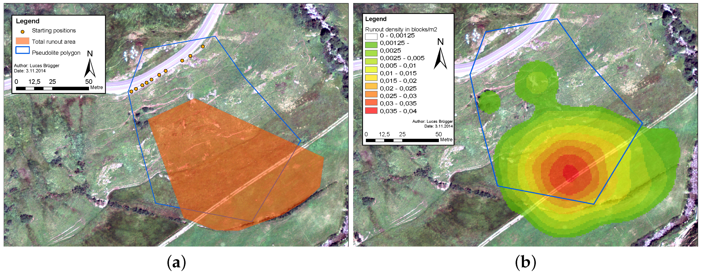
Figure 6.
(a) Start and end positions of trajectories sorted according to their starting point. (b) Distribution of obtained shadow angles in 2% steps.
Figure 6.
(a) Start and end positions of trajectories sorted according to their starting point. (b) Distribution of obtained shadow angles in 2% steps.

Figure 7.
Boxplot of the runout of (a) trajectories regarding their starting points and (b) trajectories regarding the different test blocks. The left axes (blue) describe the shadow angle in degrees (the thin vertical lines visualize the full ranges, the horizontal lines within the boxes show the medians and the upper and lower edges of the boxes are the 25% and 75% percentiles). The right axes (red) give the median of the shadow angle in percent. The linearity of the right axes does not go along with the linearity of the left axes due to their correlation .
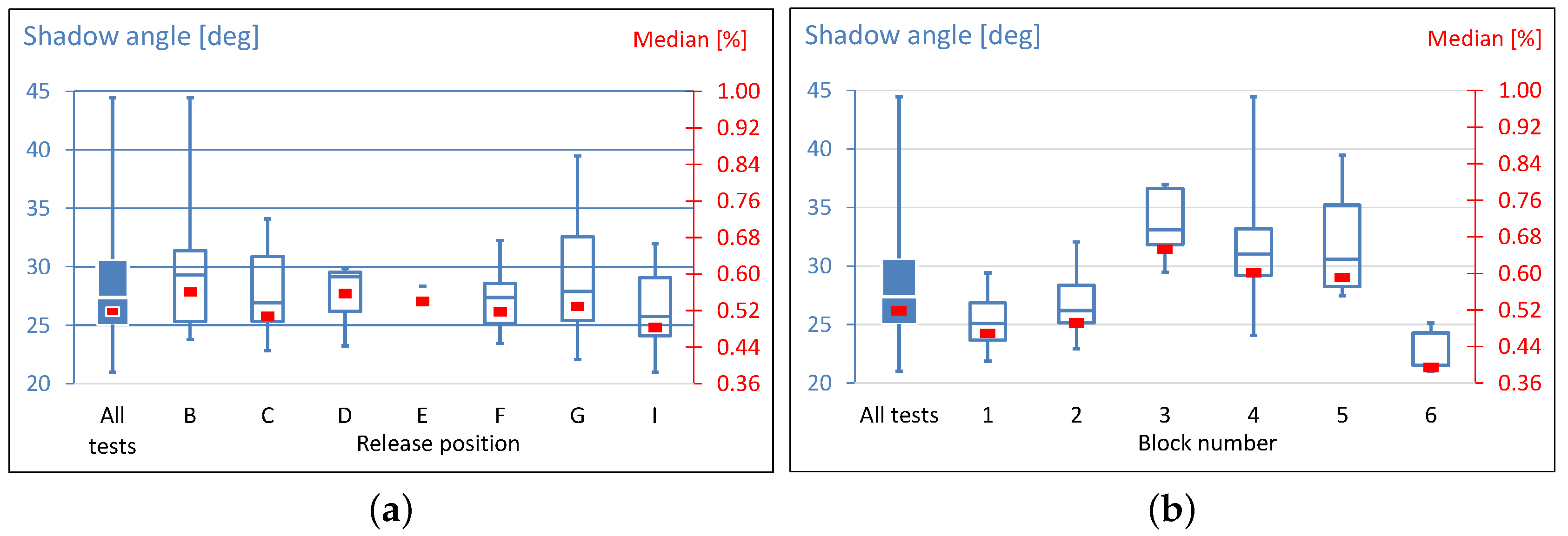
Figure 8.
The different video views: (a) the whole test slope from the opposite valley side; (b) oblique view to the steep hill section of the test slope and (c) lateral view of a block in the runout zone. The subfigures give an impression on the difficulties if a block has to be identified: in (a,b) the block is barely visible whereas (c) shows a well visible block.

Figure 9.
2D video analysis: (a) targets along the slope were identified (blue squares) and connected pairwise as exemplified for Test 7. The block positions (yellow dots) and frame numbers were recorded where blocks crossed the connection lines (dashed lines). The position of blocks in the field was determined based on the conversion factor calculated from the distance between two targets; (b) the vertical pixel position of the block during–for example–Test 28 was tracked over time. The conversion factor from pixels to meters is calculated such that the vertical parabola corresponds to a free fall sequence, with gravity as constant acceleration.

Figure 10.
Comparison of the different trajectory measuring methods of tests 7, 9 and 63 projected onto a horizontal basis projected according to CH1903 coordinate system: dashed lines represent straight connections between start and end points, continuous lines show paths obtained from video analysis and dots show point clouds from the LPS system.

Figure 11.
Example for the x- and y positions of one trajectory over time (Test 9) obtained from LPS system projected onto a virtual horizontal ground: (a) direct LPS output; (b) manual removal of singularities; (c) moving average of 0.4 s intervals; (d) median using 0.2 s intervals.
Figure 11.
Example for the x- and y positions of one trajectory over time (Test 9) obtained from LPS system projected onto a virtual horizontal ground: (a) direct LPS output; (b) manual removal of singularities; (c) moving average of 0.4 s intervals; (d) median using 0.2 s intervals.

Figure 12.
Example rockfall Test 9 showing the horizontally projected velocity over time for different median intervals 0.2 s, 0.4 s and 0.8 s.
Figure 12.
Example rockfall Test 9 showing the horizontally projected velocity over time for different median intervals 0.2 s, 0.4 s and 0.8 s.

Figure 13.
Example (Test 9) for the measured (a) rotational velocities and (b) accelerations.

Figure 14.
Example (Test 7) for the effect of a Butterworth Filter on the measured accelerations (accelerations in three dimensions were combined using Pythagoras’ theorem). In addition the rotational velocity has been plotted to visualize its relation to impacts.
Figure 14.
Example (Test 7) for the effect of a Butterworth Filter on the measured accelerations (accelerations in three dimensions were combined using Pythagoras’ theorem). In addition the rotational velocity has been plotted to visualize its relation to impacts.
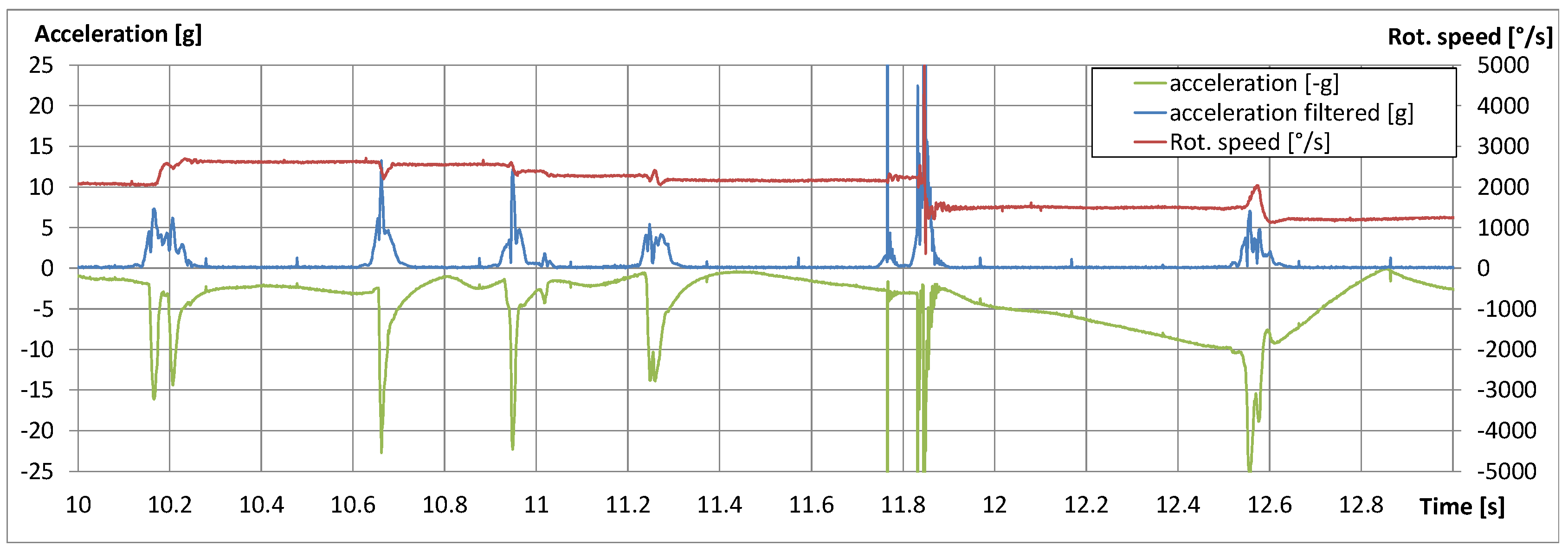
Figure 15.
Example (Test 67) of the effect of accelerometer position eccentric to the centre of mass of the block: during high rotational speeds the acceleration is high during airborne jumps. Measured acceleration is transformed (multiplied by ) and shown on the negative scale to improve the readability of the figure.
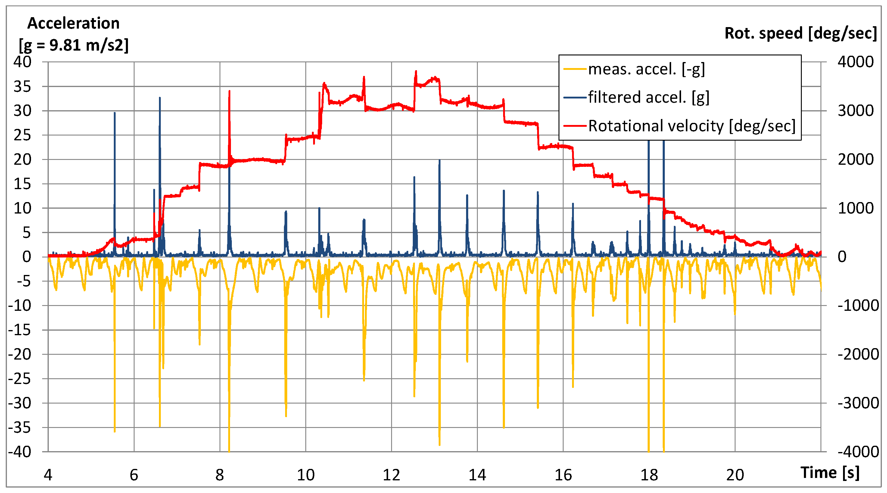
Figure 16.
A single impact during Test 109, detected by installed seismo array loggers: on the left the signals detected by three synchronized logger stations are shown over time; on the right the estimated impact location is shown with respect to the location of the logger stations (source: M. Dietze, GFZ Potsdam).
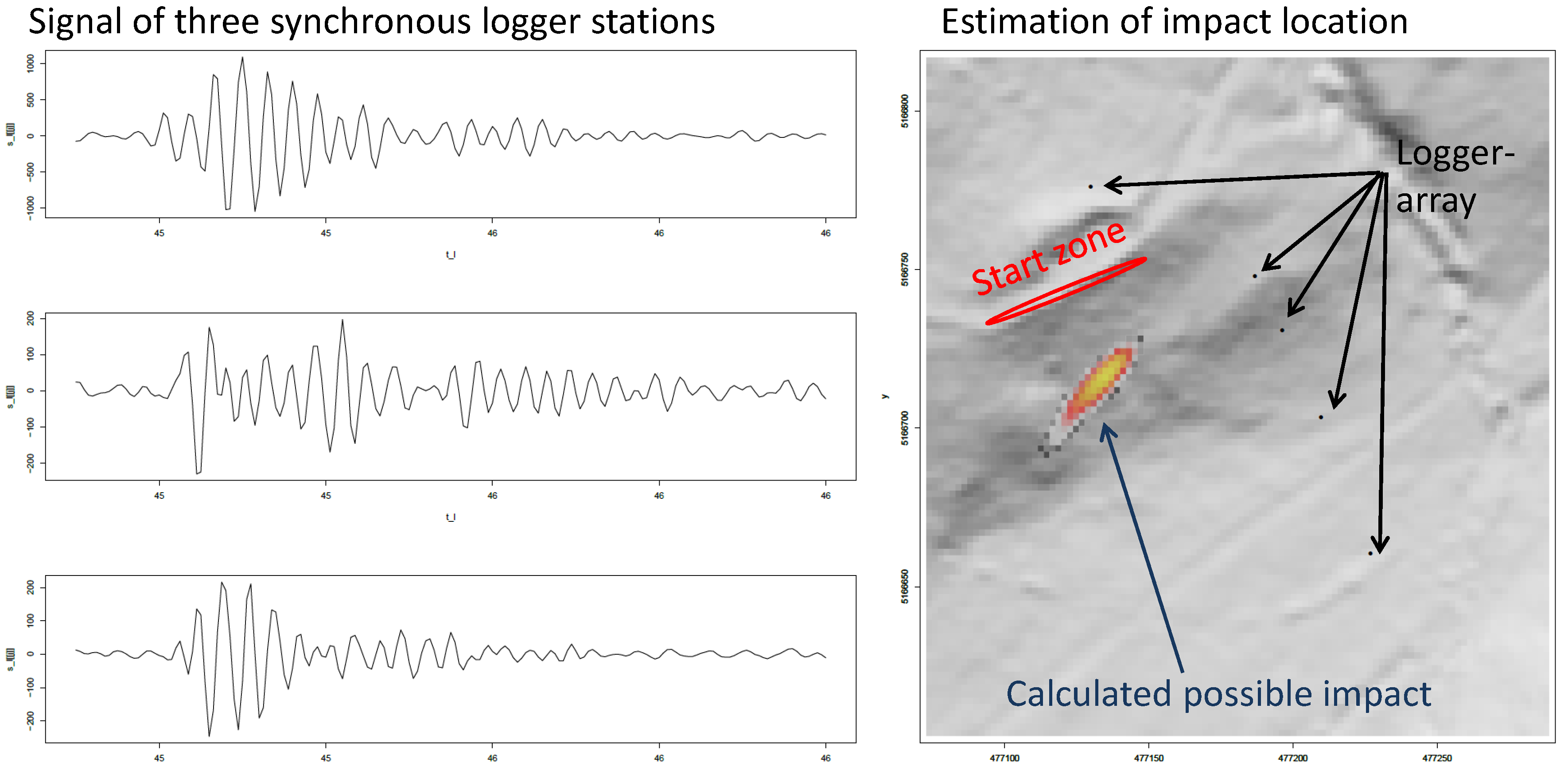
Figure 17.
Calculation of the horizontally projected block position: The real position in the field is calculated relative to the internal 2D layer of the LPS; the xy position is then calculated relative to the overall coordinate system.
Figure 17.
Calculation of the horizontally projected block position: The real position in the field is calculated relative to the internal 2D layer of the LPS; the xy position is then calculated relative to the overall coordinate system.
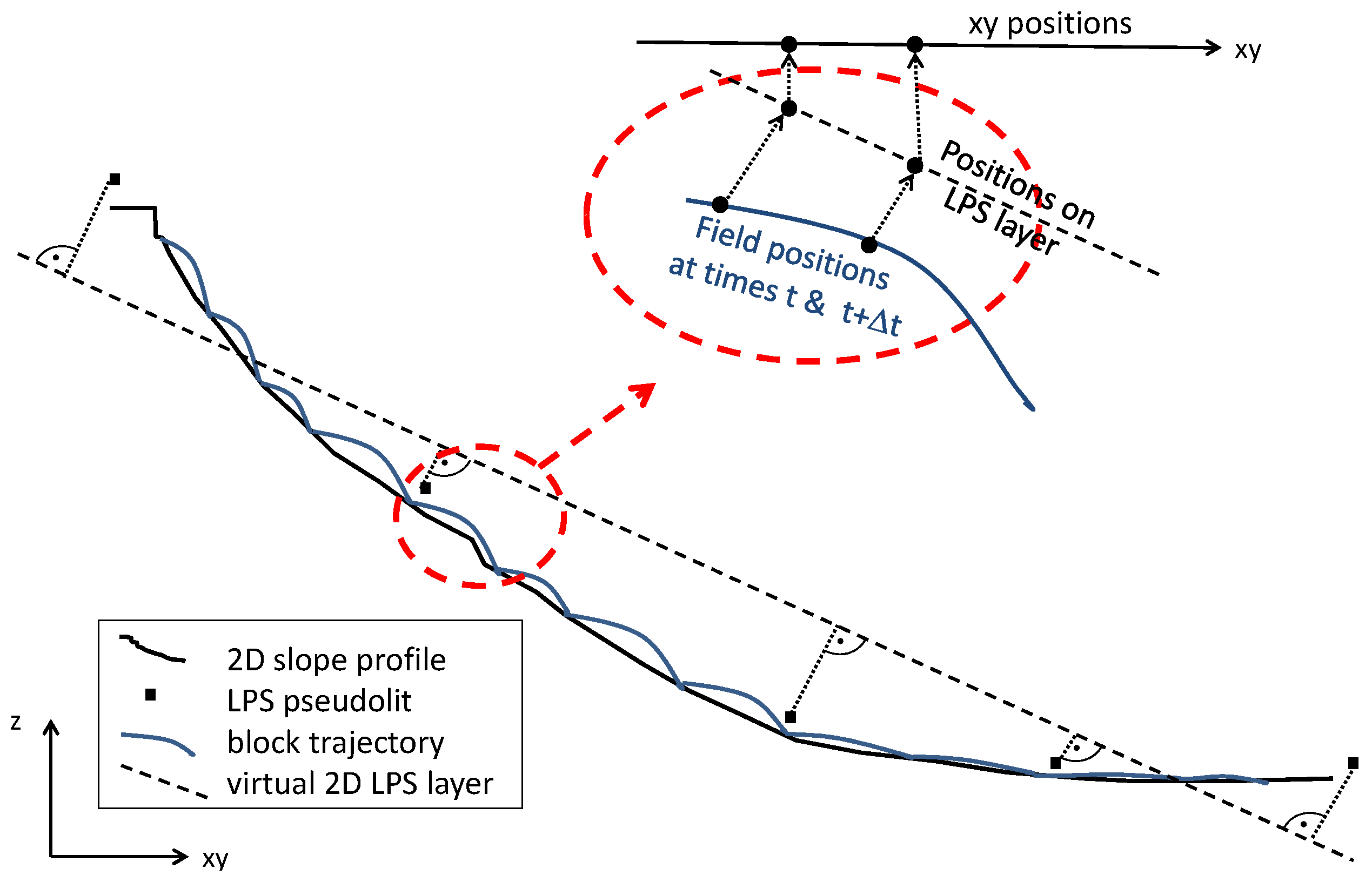
Figure 18.
Rockfall simulation of the Oberalp test site using the Unity Rockfall Model as described in Sala et al. [35] (source: Zac Sala). The same simulation using an irregular round shape delivered a mean runout of 91.8 m.
Figure 18.
Rockfall simulation of the Oberalp test site using the Unity Rockfall Model as described in Sala et al. [35] (source: Zac Sala). The same simulation using an irregular round shape delivered a mean runout of 91.8 m.
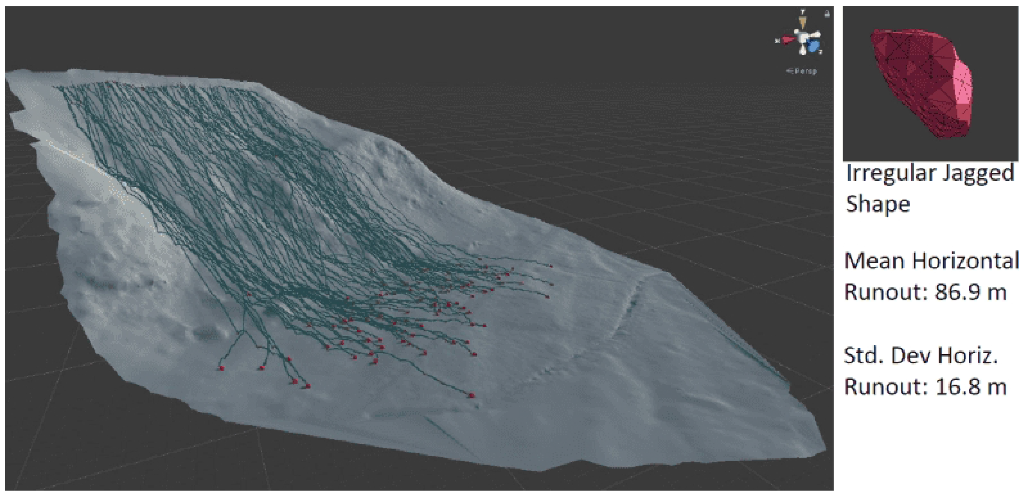

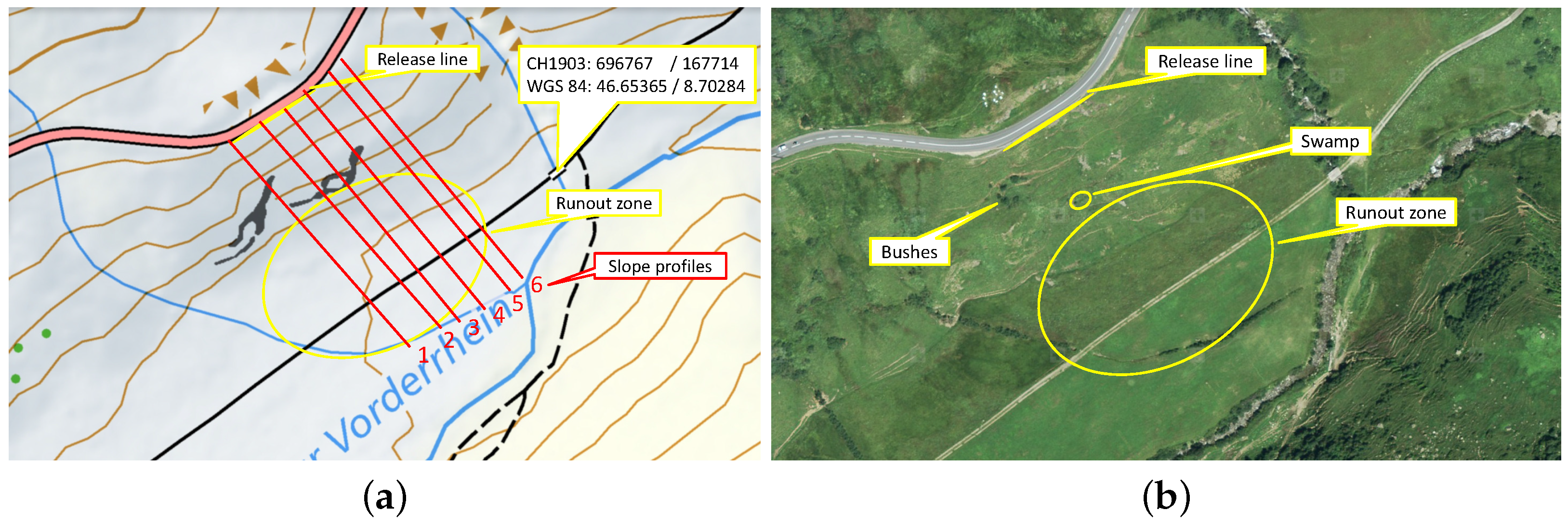
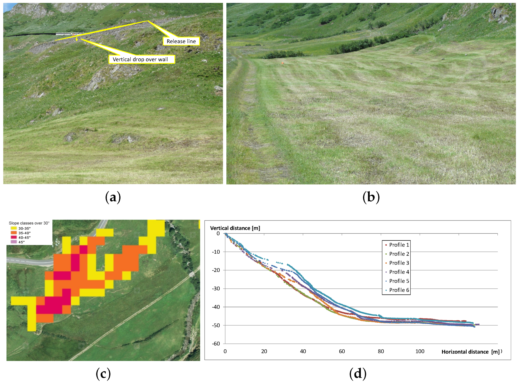
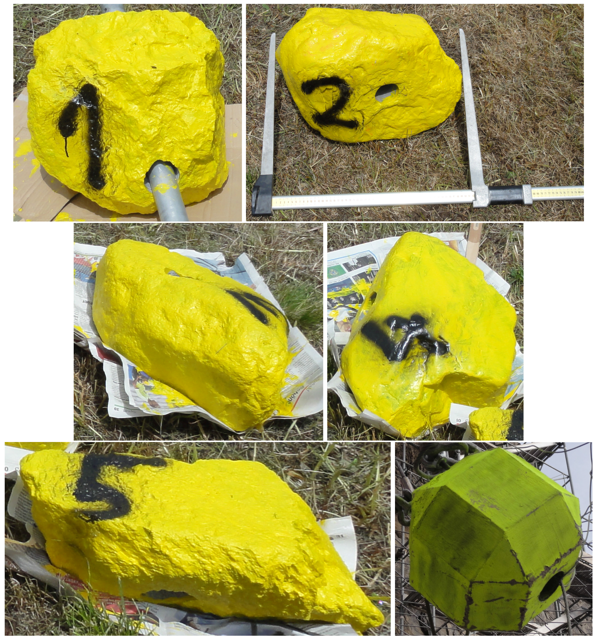
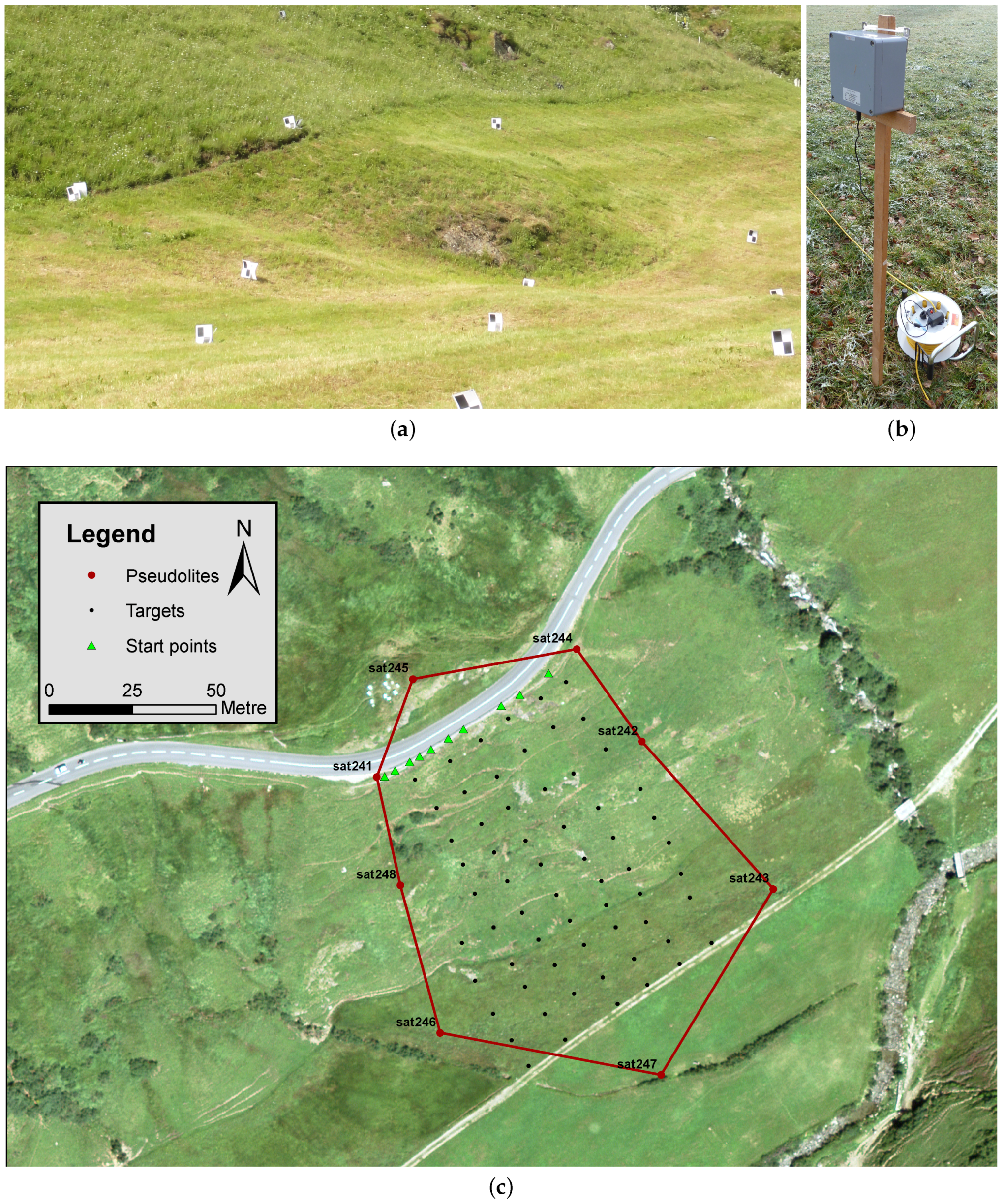
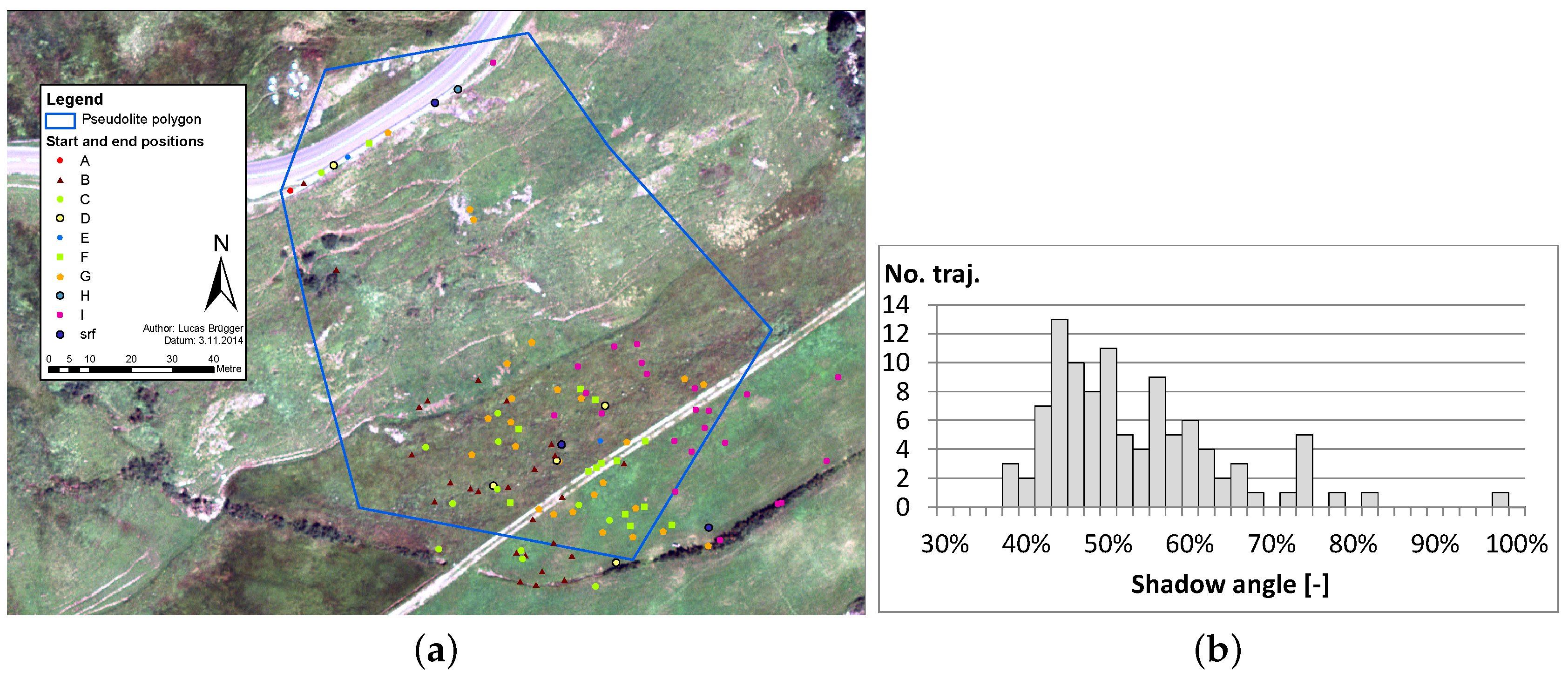
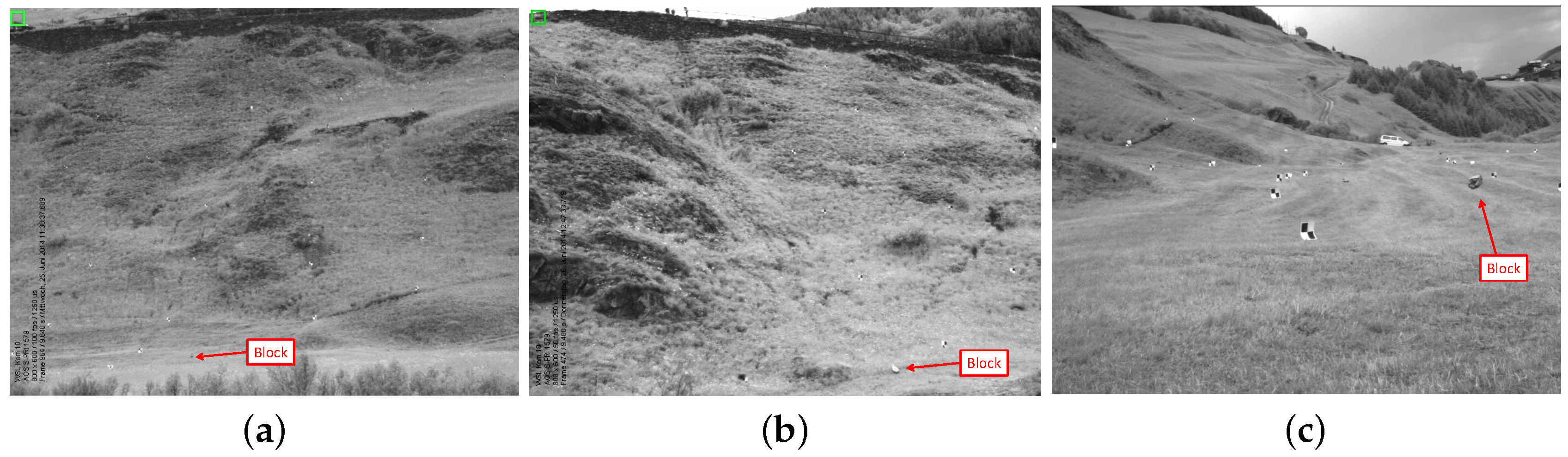
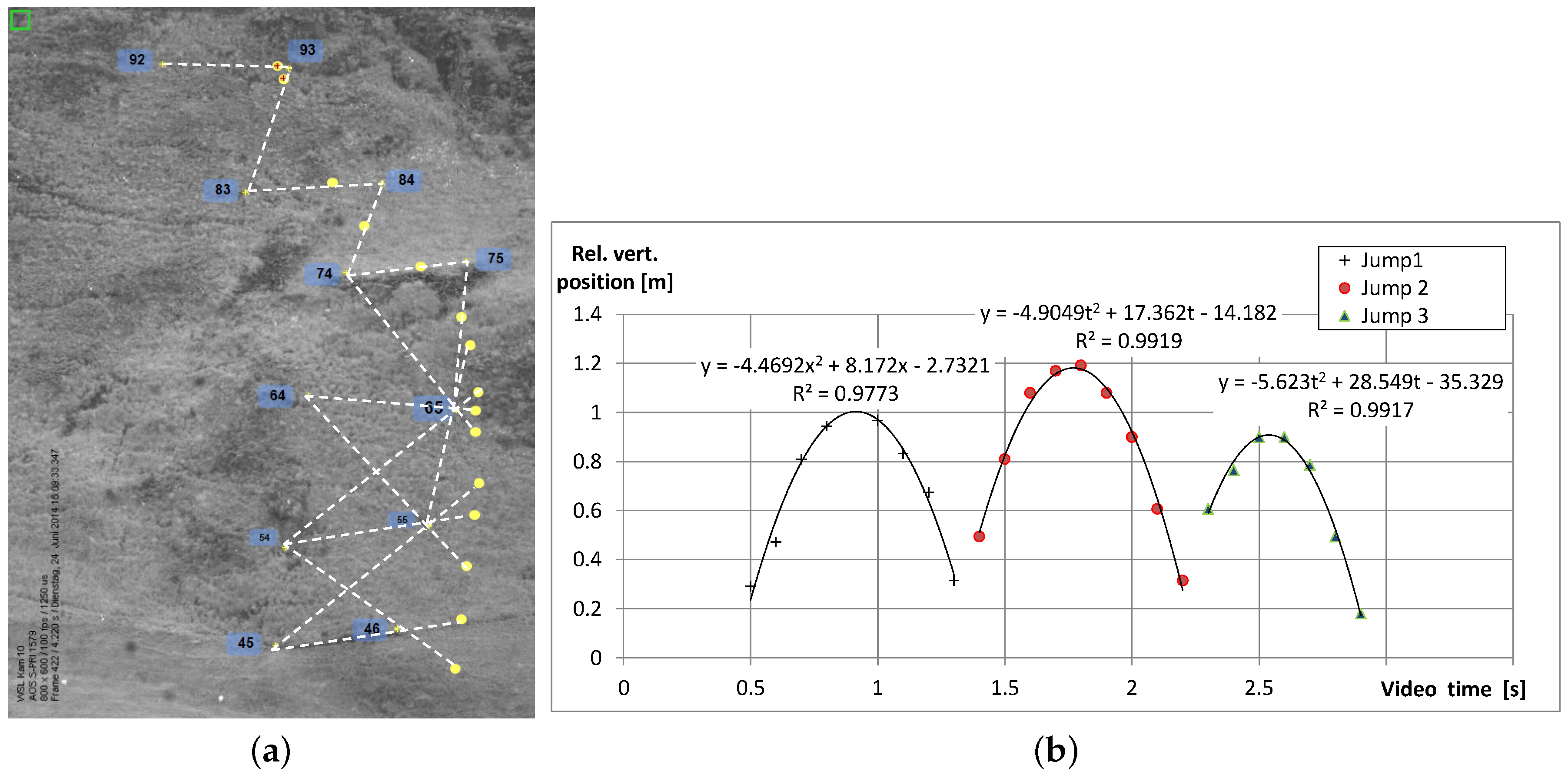
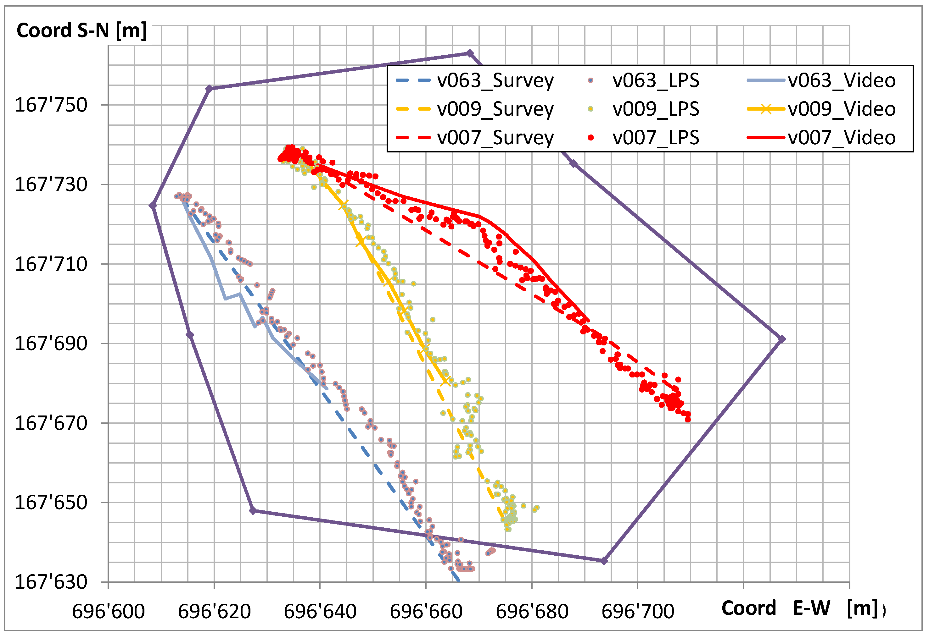
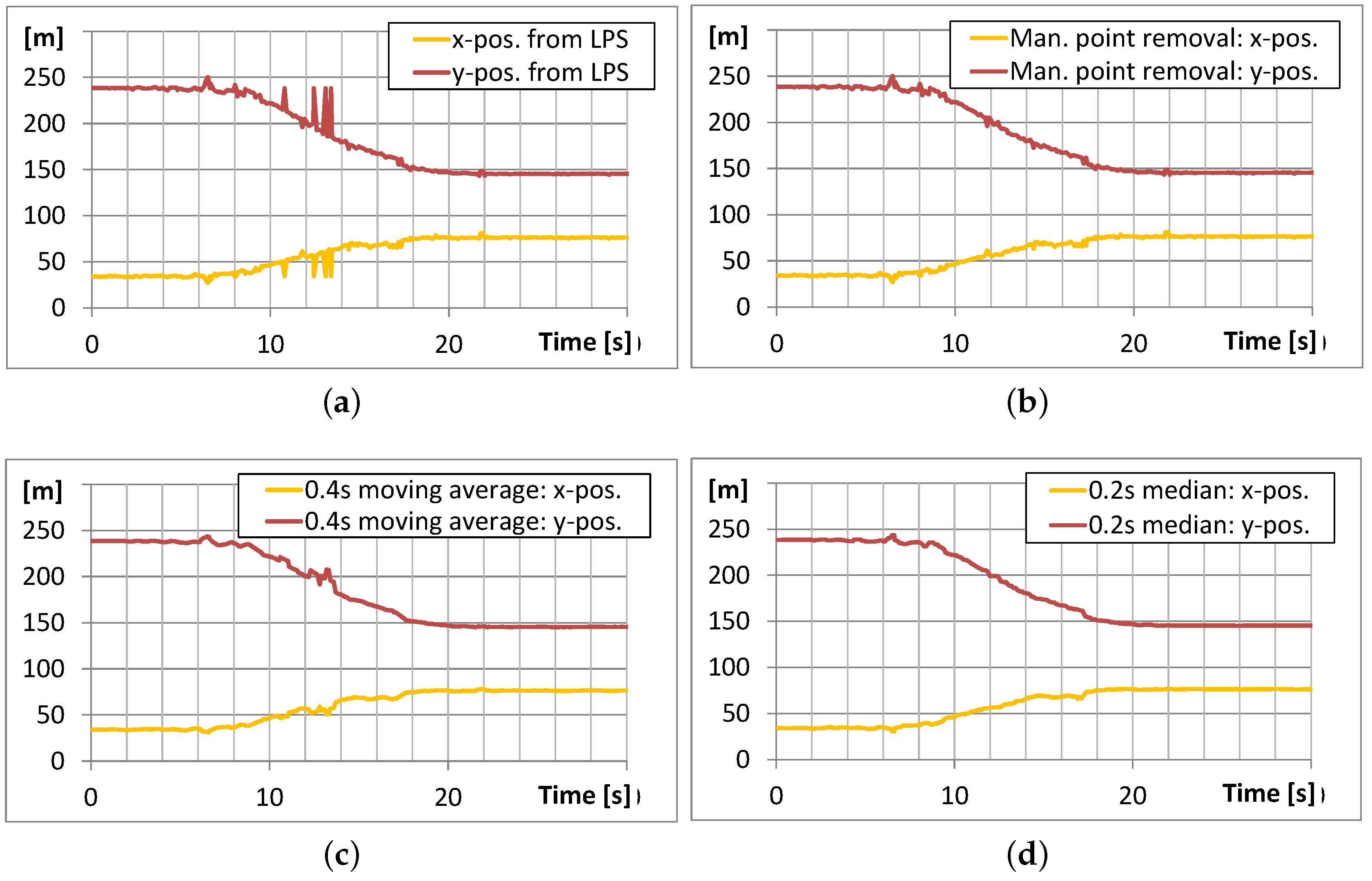
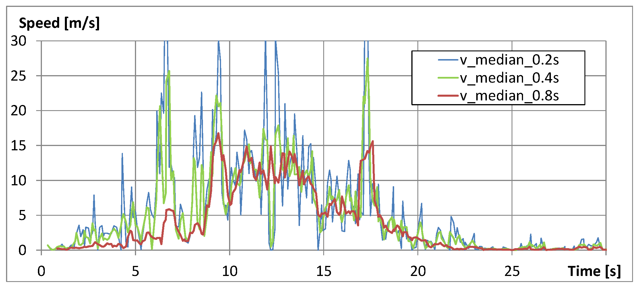
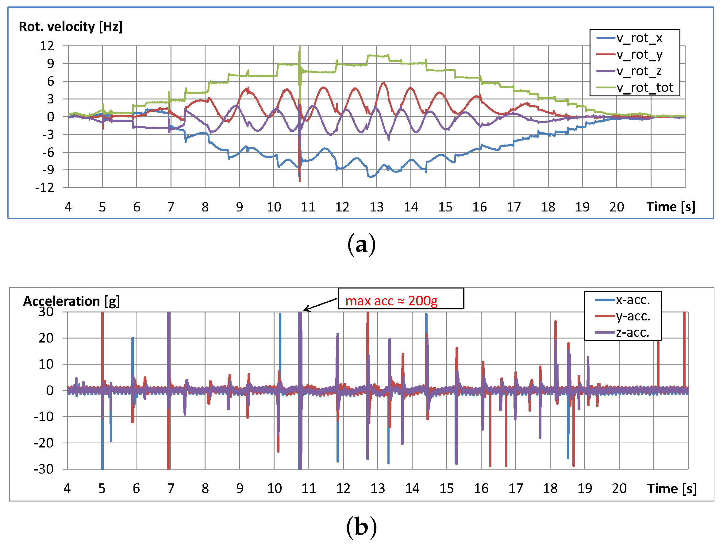
Table 1.
Rockfall release positions given in CH-1903 coordinates.
| Release Position | X | Y | Z |
|---|---|---|---|
| A | 2.70 | 89.84 | 80.50 |
| B | 5.85 | 91.64 | 80.19 |
| C | 10.18 | 94.21 | 80.03 |
| D | 13.17 | 95.93 | 79.81 |
| E | 16.56 | 98.01 | 79.53 |
| F | 21.82 | 101.27 | 79.09 |
| G | 26.33 | 104.04 | 78.65 |
| H | 43.28 | 114.34 | 77.16 |
| I | 51.87 | 120.82 | 76.34 |
| Offset | +696,608 | +167,635 | +1600 |
| (to be added to above coordinates) | |||
Table 2.
Masses and geometrical details of test specimen.
| Block Number | 1 | 2 | 3 | 4 | 5 | 6 | |
|---|---|---|---|---|---|---|---|
| Material | Gneis | Lime | Gneiss | Gneiss | Gneiss | Concrete | |
| Mass | kg | 68.7 | 78.7 | 43 | 40.3 | 19.3 | 45 |
| Dimensions | cm | 37 | 50 | 53 | 46 | 40 | 30 |
| cm | 37 | 39 | 29 | 30 | 25 | 30 | |
| cm | 32 | 30 | 20 | 20 | 18 | 30 | |
| Aspect ratio | 1.2 | 1.7 | 2.7 | 2.3 | 2.2 | 1.0 | |
| Total volume | liter | 25.9 | 30.5 | 16.2 | 14.2 | 8.3 | 19.0 |
| Length borehole | mm | 313 | 269 | 170 | 286 | 162 | 300 |
| Diameter borehole | mm | 69 | 69 | 69 | 69 | 69 | 70 |
| Volume borehole | liter | 0.70 | 0.60 | 0.38 | 0.64 | 0.36 | 0.69 |
| Netto volume | liter | 25.20 | 29.90 | 15.82 | 13.56 | 7.94 | 18.31 |
| Material density | kg/liter | 2.73 | 2.63 | 2.72 | 2.97 | 2.43 | 2.46 |
| Average density (with borehole) | kg/liter | 2.65 | 2.58 | 2.65 | 2.84 | 2.33 | 2.37 |
Table 3.
Performed experiments for different release position combinations A–I and blocks 1–6. All trajectories were classified regarding their quality ranging from good “+”, medium “o” and poor “-”.
Table 3.
Performed experiments for different release position combinations A–I and blocks 1–6. All trajectories were classified regarding their quality ranging from good “+”, medium “o” and poor “-”.
| Block Number | 1 | 2 | 3 | 4 | 5 | 6 |
|---|---|---|---|---|---|---|
| Release position | ||||||
| A | ||||||
| B | ++++ | ++++ | oo | o+++ | ||
| +-+- | ++++ | +o-++ | ||||
| C | ++o- | +++ | + | +++ | ||
| D | o | - | o | |||
| E | + | |||||
| F | o-o | +++ | o | ooo | oo | |
| o++ | ++ | o+ | ||||
| G | o++o | +++ | oo | o++ | -o+ | |
| -++ | +++ | ++- | ++ | |||
| I | +++ | +++ | o+++ | ++++ | - - - | |
| ++ | ++ | o+- | ||||
| Comment | no live position | no live position | no live position | |||
| no rock sensor | no rock sensor |
Table 4.
Overview of the measurements of full trajectories. Collective results from multiple blocks: runout characteristics calculated based on 102 rockfall tests; travel times and averaged speeds calculated from 73 trajectories.
Table 4.
Overview of the measurements of full trajectories. Collective results from multiple blocks: runout characteristics calculated based on 102 rockfall tests; travel times and averaged speeds calculated from 73 trajectories.
| Horizontal Distance [m] | Vertical Distance [m] | Shadow Angle | Travel Time [sec] | Average Speed | |||
|---|---|---|---|---|---|---|---|
| [–] | [deg] | hor. [m/s] | skew [m/s] | ||||
| Minimum | 22.4 | 51.4 | 38% | 21.0 | 11.5 | 2.1 | 2.4 |
| Maximum | 128.1 | 22.0 | 98% | 44.5 | 43.2 | 5.5 | 6.1 |
| Mean | 92.8 | 48.2 | 54% | 28.3 | 23.4 | 4.2 | 4.7 |
| Median | 95.6 | 49.2 | 52% | 27.4 | 23.5 | 4.2 | 4.7 |
| Std. dev. | 20.1 | 4.7 | 11% | 4.5 | 3.3 | 0.6 | 0.6 |
Table 5.
Comparison of single results of redundant measurements during Test 109 during three jumps in the runout zone between 15 s and 17 s. The comparison between the two different measurements is given by the absolute difference and the percentage with respect to the measured/derived value, which was considered to be more reliable.
| Jump | Rockfall Sensor | Video Analysis | LPS | max. Diff. | |||
|---|---|---|---|---|---|---|---|
| 1 | Rotational speed [/s] | 2758 | 2571 | 187 | = | 7% | |
| 2 | 2192 | 2250 | 58 | = | 3% | ||
| 3 | 2031 | 2000 | 31 | = | 2% | ||
| 1 | Jump duration [s] | 0.49 | 0.5 | 0.01 | = | 2% | |
| 2 | 0.7 | 0.7 | 0.0 | = | 0% | ||
| 3 | 0.72 | 0.7 | 0.02 | = | 2% | ||
| 1 | Velocity [m/s] | 10.7 | 9.6–10.4 | 1.1 | = | 10% | |
| 2 | 8.4 | 5.6–10.4 | 2.8 | = | 33% | ||
| 3 | 7.4 | 5.6–7.9 | 1.8 | = | 24% | ||
| 1–2 | Impact acceleration [m/s] | 76 | 60 | 16 | = | 21% | |
| 2–3 | 46 | 36 | 10 | = | 22% | ||
© 2018 by the authors. Licensee MDPI, Basel, Switzerland. This article is an open access article distributed under the terms and conditions of the Creative Commons Attribution (CC BY) license (http://creativecommons.org/licenses/by/4.0/).
Share and Cite
MDPI and ACS Style
Volkwein, A.; Brügger, L.; Gees, F.; Gerber, W.; Krummenacher, B.; Kummer, P.; Lardon, J.; Sutter, T. Repetitive Rockfall Trajectory Testing. Geosciences 2018, 8, 88. https://doi.org/10.3390/geosciences8030088
AMA Style
Volkwein A, Brügger L, Gees F, Gerber W, Krummenacher B, Kummer P, Lardon J, Sutter T. Repetitive Rockfall Trajectory Testing. Geosciences. 2018; 8(3):88. https://doi.org/10.3390/geosciences8030088
Chicago/Turabian StyleVolkwein, Axel, Lucas Brügger, Fabio Gees, Werner Gerber, Barbara Krummenacher, Peter Kummer, Jessica Lardon, and Tobias Sutter. 2018. "Repetitive Rockfall Trajectory Testing" Geosciences 8, no. 3: 88. https://doi.org/10.3390/geosciences8030088
Note that from the first issue of 2016, this journal uses article numbers instead of page numbers. See further details here.