Unified Geomorphological Analysis Workflows with Benthic Terrain Modeler

Esri (Software Company); 380 New York St., Redlands, CA 92373, USA
*
Author to whom correspondence should be addressed.
Geosciences 2018, 8(3), 94; https://doi.org/10.3390/geosciences8030094
Submission received: 18 January 2018
/
Revised: 7 March 2018
/
Accepted: 8 March 2018
/
Published: 11 March 2018
(This article belongs to the Special Issue Marine Geomorphometry)
Abstract
:High resolution remotely sensed bathymetric data is rapidly increasing in volume, but analyzing this data requires a mastery of a complex toolchain of disparate software, including computing derived measurements of the environment. Bathymetric gradients play a fundamental role in energy transport through the seascape. Benthic Terrain Modeler (BTM) uses bathymetric data to enable simple characterization of benthic biotic communities and geologic types, and produces a collection of key geomorphological variables known to affect marine ecosystems and processes. BTM has received continual improvements since its 2008 release; here we describe the tools and morphometrics BTM can produce, the research context which this enables, and we conclude with an example application using data from a protected reef in St. Croix, US Virgin Islands.
Data Set License: CC-BY
1. Introduction
The marine environment is under heavy pressure from a host of human activities, with a large portion of the system strongly impacted by anthropogenic threats [1]. At the same time, our understanding of the ocean suffers from a paucity of data detailing its inner workings, with little mapped in detail [2]. While satellite derived gravity data has increased the nominal resolution of global bathymetry data to 30 arc-seconds [3], and recent efforts have mapped global marine units [4], these data are unable to resolve finer-scale oceanic processes. Applications in seascape ecology, marine spatial planning, morphological evolution, and understanding human ocean uses require higher resolution data [5]. Where terrestrial applications can rely on global-scale coverage from low cost remote sensing platforms, ocean observations have relied on local-scale ship borne or in situ sensor based platforms, with high data acquisition costs and limited swath width. Recent technological advances have lowered costs and increased the extent and quality of bathymetry and a small but growing portion of the ocean is becoming well mapped. Habitat mapping is a first step to further our understanding of the ocean environment, and is typically informed by bathymetric gradients, which influence species abundance and distribution [6,7]. Geomorphic derivatives can be used to infer the effects of bathymetric gradients, increasing the value of limited data. The geomorphic derivatives are often used directly as a measure of the environment, or as covariates in predictive models. Increased availability of bathymetric data has led to new methodologies to infer bathymetric gradients from geomorphic derivatives and map seafloor habitat [8]. Because geomorphometry lacks a formalized unifying theory [9], a single approach is not yet possible. With consistent methodologies and better understanding of the algorithms in use, the field will lend itself more readily to expanding understanding of our oceans.
Today, modern seafloor mapping technologies such as light detection and ranging (LiDAR) and multibeam bathymetry have done much to lower the costs, and provide consistent bathymetric products which incorporate in-sensor error models, provide high point density, and accurate georeferencing making them suitable for scientific analysis [10,11]. Bathymetric data are often captured, processed to remove artifacts and errors, and integrated into a consistent geomorphological model. Creation and interpretation of such a model has been aided by geomorphometry analysis tools in packages such as Benthic Terrain Modeler (BTM) [12,13]. BTM is built on top of the popular ArcGIS platform, is open source, has an intuitive interface, and has received continual development. When BTM was first introduced in 2006, transforming collected data to research results required mastery of many different pieces of software.
Recent methodological developments have reduced the complexity of doing such analysis, but this has coincided with the emergence of even more sophisticated tools and the ability to collect much higher resolution data. Here, we describe the tools provided with the current release of BTM (v3.0), and highlight how it can be used in powerful analytical workflows for seafloor classification, by combining it with the capabilities of ArcGIS, the Python scientific stack, and the R statistical programming language. As the sphere of scientific software continues to grow, it will be important to provide easy-to- use tools to aid the broader community in performing rigorous analysis of marine geomorphometry.
2. Materials and Methods
Bathymetric digital terrain models (DTMs) are commonly used in three morphometric applications: deriving terrain attributes, seafloor classification, and object detection [11]. BTM is used for both terrain attribute creation and seafloor classification. Researchers have adopted BTM to create terrain attributes (e.g., [14,15,16]) for use as covariates to predictive modeling applications. BTM is also used for performing semi-automated classified seafloor mapping. By combining the bathymetric position index (BPI; see Section 2.1.2) with slope and depth, BTM provides a simple tool which maps ranges of these terrain attributes to a classification dictionary. This can be used to identify benthic zones (e.g., crests, depressions, flats and slopes) [17], but also to provide more detailed habitat maps, with the additional step of empirical evaluation of the relationship between the terrain attributes in use and the species of interest.
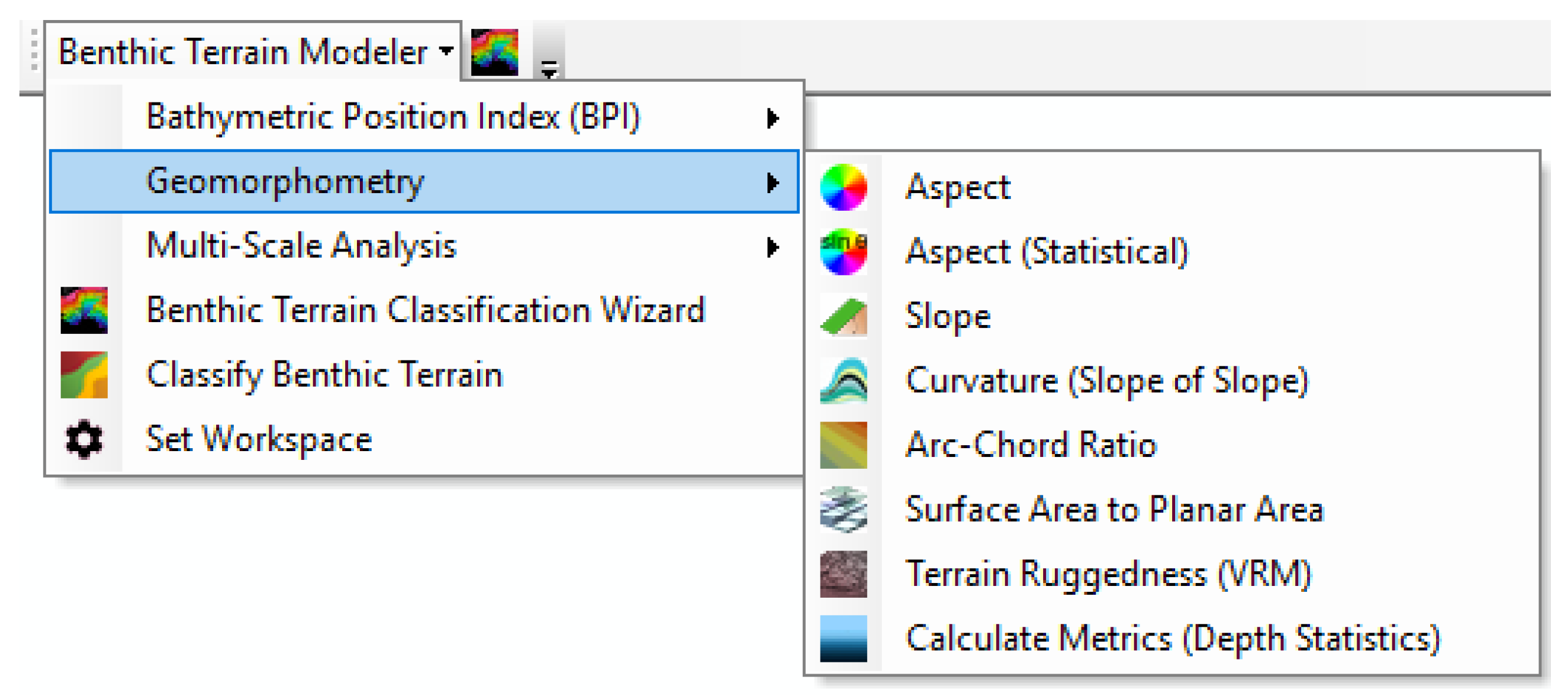
The following section describes the algorithms implemented by BTM (see Table 1), which cover a broad swath of use cases, and span five classes of terrain attributes: (1) Surface gradients, computed from cell neighborhoods, form the foundation of raster analysis. BTM includes basic gradients implemented by the ArcGIS extension Spatial Analyst, and complements these with specialized gradients useful for geomorphometry; (2) Measures of relative position are closely tied to many physical and biological processes, and provide useful information on both habitat and suitability; (3) Measures of surface roughness, or rugosity, quantify local heterogeneity and are important for understanding seafloor composition; (4) Distributional moments capture statistical measures of the terrain and include simple statistics like mean and variance, but also more complex measures like kurtosis; (5) Multidimensional tools assist with the important step of determining the appropriate scale of analysis.
2.1. Marine Geomorphometry Algorithms
2.1.1. Surface Gradients
The surface gradient provides valuable information for environmental applications of DTMs. Slope and aspect form a gradient representing the first order derivative of the surface, and are implemented in ArcGIS and BTM using the method of Horn [18], which uses a neighborhood (also known as the Moore neighborhood [25]) for its analysis, operating on a planar surface. Instead of using the Moore neighborhood, a quadratic can also be fitted to the surface at the point of interest. The Wood-Evans method [26,27] implements this approach to slope, and can be computed at arbitrary window sizes. The algorithm is implemented in Jo Wood’s Landserf [27], and is also available in ArcGIS with the ArcGeomorphometry extension [28]. Dolan et al. [29] compare slope algorithms for benthic geomorphometry and the effects of scale on the results, and recommend both the Horn and Wood-Evans methods for capturing slope in planar bathymetric data over other available methods.
Geodesic slope: In 2017, ArcGIS added support for computing slope on a geodesic. Instead of computing the results in a Cartesian plane, the geodesic method computes directly on the ellipsoid [30]. It retains the use of a neighborhood, but improves on the planar method by measuring the angle between the surface and the geodetic datum for each of the 8 adjacent cells, and is fitted with least squares described in Figure 1. This produces more accurate results, particularly when used in conjunction with new high resolution bathymetry sensors with low positional uncertainty [10]. For typical sonar and lidar applications, the positional uncertainty of the observations and the effects of creating a DEM surface will be primary determinants in the accuracy of the slope calculation.
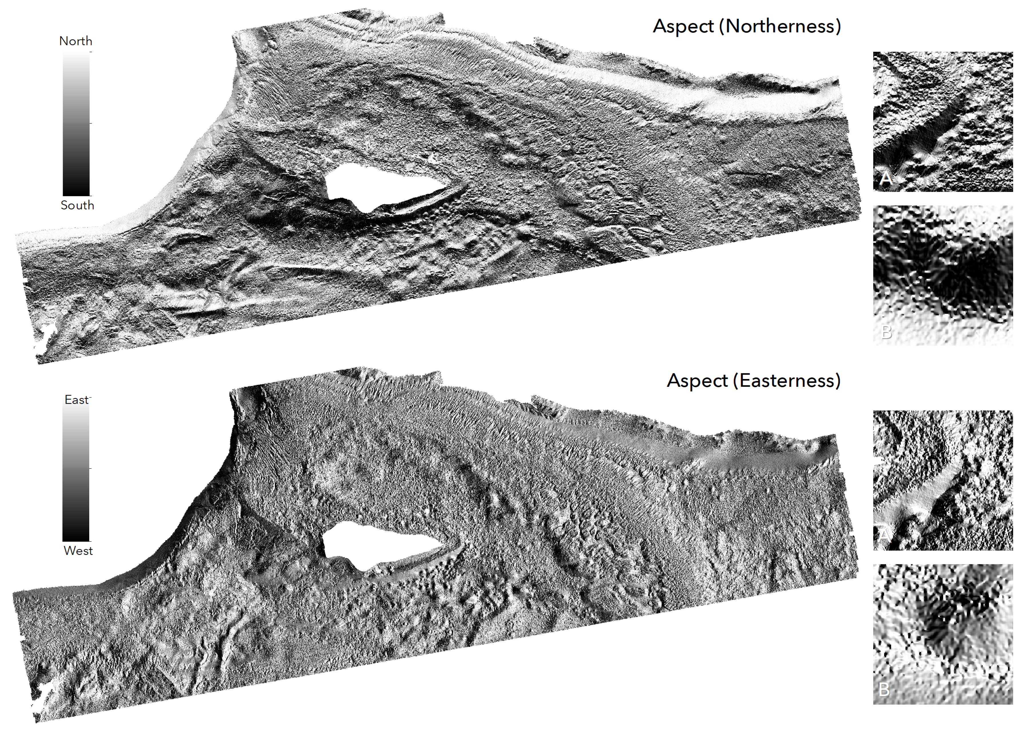
Aspect: Aspect measures surface direction. In ArcGIS, it ranges from 0 to 359.9 degrees, measured clockwise from north, and −1 for locations of no slope, based on the same Horn [18] method. BTM augments this with an additional aspect calculation, which converts aspect into two variables: Northerness , due south to due north, and easterness , due west to due east [19,20].
This transformation is beneficial in many modeling contexts where circular variables violate the model constraints, and these two linear scaled derivatives are commonly used in models such as in Lecours et al. [31] and Davies et al. [32]. Results of this transformation are shown in the center and bottom panels of Figure 2.
2.1.2. Curvature/Relative Position
Analyzing the rate of change of the slope is linked to both physical and biological processes [12,34,35]. Physically these attributes can affect marine flow, internal waves and current channeling. Biologically, these attributes largely determine exposure, and are often a useful proxy of habitat suitability [36]. BTM uses the existing ArcGIS implementation for curvature, and implements two methods of computing relative position: bathymetric position index (BPI) and the relative difference to the mean.
Curvature: Curvature is the second derivative of the bathymetric surface, or the first derivative of slope, computed in ArcGIS using the method of Zevenbergen et al. [37]. Curvature is evaluated by first calculating the second derivative for each cell in the surface using a moving window, and then fitting a fourth order polynomial to the values within the window (see Figure 1). Curvature evaluated only parallel to the slope (profile curvature) can describe the acceleration or deceleration of benthic flow, while curvature evaluated perpendicular to slope (planiform curvature) can help describe convergence or divergence of flow.
Bathymetric Position Index: BPI is a marine focused version of the Topographic position index (TPI) [38] which classifies landscape structure (e.g., valleys, plains, hill tops) based on the change in slope position over two scales. BPI quantifies where a location on a bathymetric surface is relative to the overall seascape [12]. For each cell in a surface, BPI is evaluated by finding the difference between the elevation value of the cell and the mean elevation of all cells in an annulus (a ring shape bounded by two concentric circles) surrounding the location. The use of an annulus allows for the exclusion of immediately adjacent cells when measuring mean surrounding elevation. The resulting values are positive near crests and ridges, and negative near cliff bases and valley bottoms.
BPI is used in the semi-automated classification provided with BTM, and has been linked to habitat preferences [39]. For a typical application, two scales of BPI are computed, the broad and fine scale BPIs. Analyzing BPI at two scales helps capture scale dependent phenomena within the data, and when matched to dominant scales, can be a simple way to incorporate basic multiscale analysis. For historical reasons BTM provides separate tools for broad and fine scale BPI, but these are the same algorithm internally, and future releases may provide automated multiscale analysis of this parameter. As pointed out in Lecours et al. [11], further improvements may be obtained by computing this measure against a quadratic surface, and this is an area for potential improvement for BTM.
Relative difference to the mean: Relative difference to the mean measures relative position of a location using the mean of a continuous neighborhood of cells rather than an annulus. Similar to BPI, it is evaluated by finding the difference between the mean elevation of all cells in the neighborhood and the elevation of the focal cell. This difference is divided by the range of the focal neighborhood, where range is the difference between the maximum and minimum elevations in the neighborhood.
Relative difference to the mean can be an important descriptor of bathymetric structure [40]. While both relative difference to mean and BPI are measures of relative location on a surface, the two metrics showed low correlation (<0.1) at the scales used in our analysis (see Table A2). A generalized evaluation of their correlation is out of the scope of this paper, but the results suggest that the two metrics may be independently valuable as descriptors of benthic terrain.
2.1.3. Rugosity/Surface Roughness
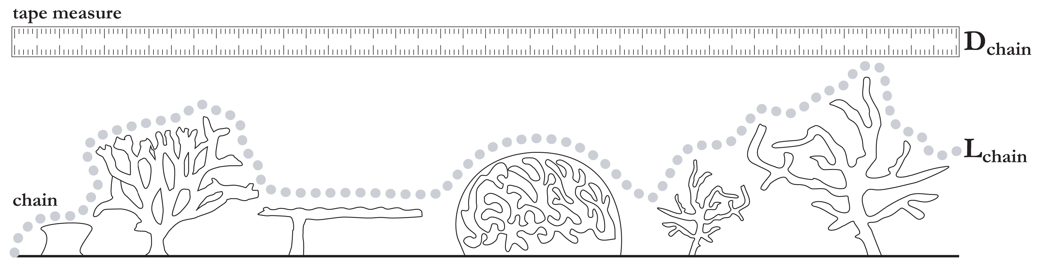
Terrain heterogeneity is an important predictor of habitat location and species density [41]. Rugosity, also known as surface roughness or complexity, is a common descriptor of terrain heterogeneity in both terrestrial and marine applications. Rugosity is traditionally evaluated in-situ across a two dimensional terrain profile by draping a chain over the surface and comparing the length of the chain with the linear length of the profile (see Figure 3).
With the widespread availability of terrestrial elevation data and the increasing availability of bathymetric surfaces, many methods of evaluating rugosity ex-situ on a three dimensional surface have been proposed. These methods measure a ratio of areas rather than lengths, as shown in Equation (3). BTM supports four methods of measuring rugosity across three tools: Surface Area to Planar Area, Vector Ruggedness Measure, and Arc-Chord Ratio.
Surface Area to Planar Area: Following the work of Jeff Jenness [23], BTM has implemented the Surface Area to Planar Area (SAPA) tool since its release. SAPA evaluates rugosity using a neighborhood, by drawing a line from the center of each cell in the window to the center of the central cell in three dimensions. The result is a network of eight triangles in the central cell which approximates the contoured surface at the cell location. The sum area of these triangles is divided by the two dimensional cell area to obtain a measure of rugosity. Because of its calculation method, SAPA is tightly coupled with slope, and is surpassed by the other methods in BTM for computing rugosity.
Vector Ruggedness Measure: Sappington at al. [22] describe a measure of surface roughness titled Vector Ruggedness Measure (VRM) that is also calculated using a moving window, based on an earlier method proposed by Hobson [43]. For each cell in the window, a unit vector orthogonal to the cell is decomposed using the three dimensional location of the cell center, the local slope, and the local aspect. A resultant vector for the window is evaluated and divided by the number of cells in the moving window. The magnitude of this standardized resultant vector is subtracted from 1 to obtain a dimensionless value that ranges from 0 (no variation) to 1 (complete variation). Typical values are small (≤0.4) in natural data.
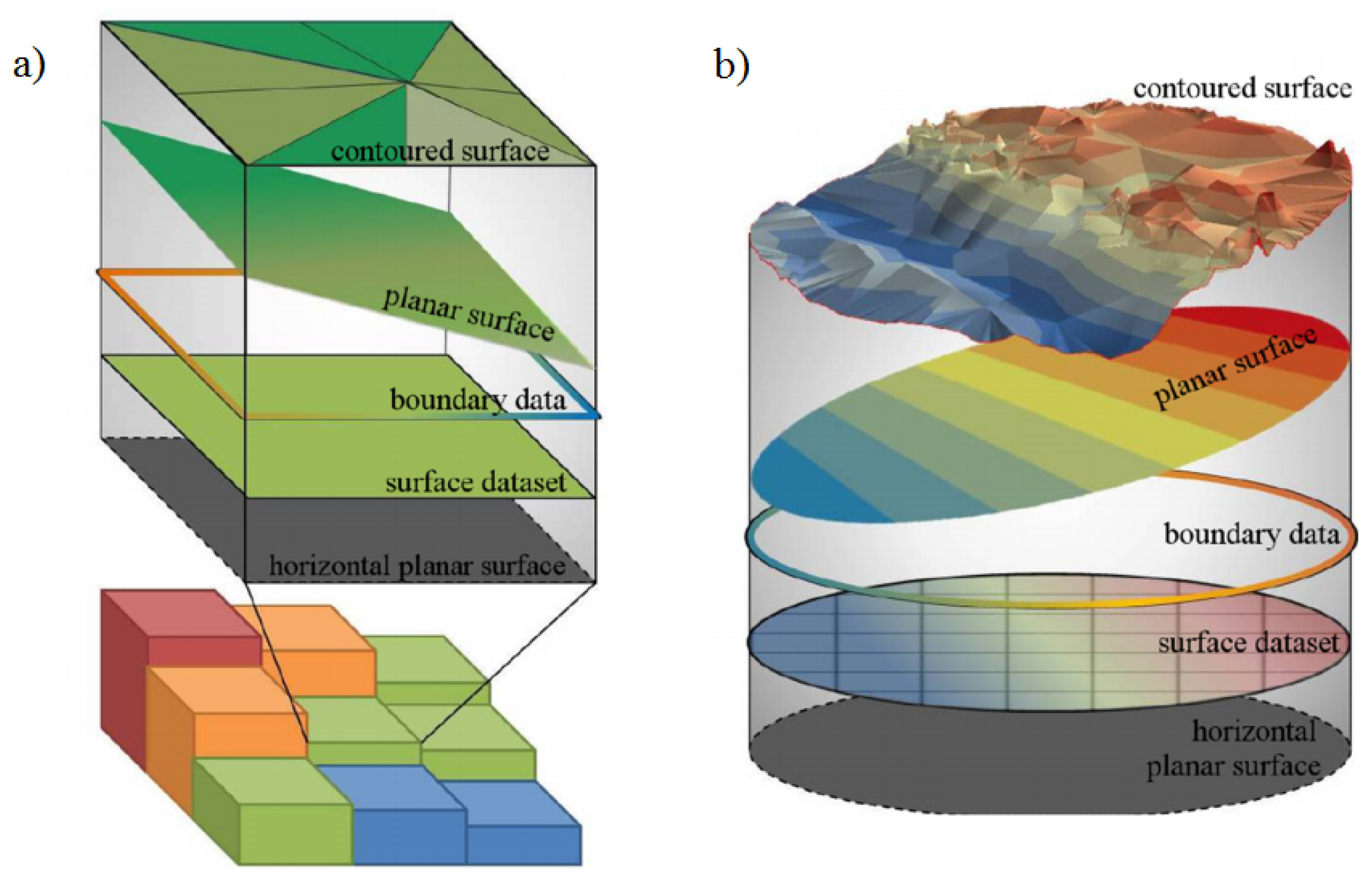
Arc-Chord Ratio: The Arc-Chord Ratio (ACR) was introduced in DuPreez [24]. Similar to Friedman et al. [42], ACR evaluates surface ruggedness using a ratio of contoured area (surface area) to the area of a plane of best fit (POBF), where the POBF is a function of the boundary data. By using a POBF rather than a horizontal plane to determine planar area, rugosity is decoupled from slope at the scale of the surface, and is being adopted as an improved measure of surface roughness [44]. DuPreez [44] provides two three dimensional methods of deriving ACR that are independent of data dimensionality and scale; both are supported by BTM.
The first method of calculating three dimensional ACR is exposed in BTM through the Arc-Chord Ratio tool, and calculates a single ACR value for an area of interest (AOI) rather than creating a surface of local ACR values. This AOI is chosen by the user based on the context and scale of the analysis, as well as the resolution of the data. The depth surface is converted to a triangulated irregular network (TIN) and clipped to the AOI. Contoured area is determined by summing the triangle areas within the TIN. Planar area is determined by fitting a POBF to the elevation values along the boundary of the AOI, using the Global Polynomial Interpolation tool in ArcGIS to obtain the fitted plane, and as shown in Figure 4. The result is a single ratio representing global ACR rugosity for the area of interest.
Surface Area to Planar Area (Slope-corrected): The second method of calculating the Arc-Chord Ratio is exposed through the Surface Area to Planar Area tool described above. By selecting the “Correct Planar Area for Slope” option, the tool will divide the contoured area by the cell area as projected onto the plane of the local slope. The result is a surface where each cell represents the local ACR rugosity.
2.1.4. Distribution Moments
In addition to specialized morphometrics, BTM computes summary statistics on neighborhoods of data. It supports both circular or square neighborhoods, internally using the neighborhood tools provided in ArcGIS. These measurements provide a spatially aggregated summary of the values within the neighborhood, and are a measure of biotic assemblage structure [45]. These are provided in BTM with the Calculate Metrics (Depth Statistics) tool. Calculate Metrics (Depth Statistics) exposes summary statistics currently available in ArcGIS with the Focal Statistics tool, as well as several statistics that have not yet been implemented in ArcGIS.
Mean is the average water depth in the neighborhood. This simple filter is frequently used to filter noise from the data collection process, but also can provide a smoothed surface which accounts for large scale variations in the DTM, and when subtracted from the DTM, provides a residual of fine scale morphologies [46]. Standard deviation captures the local dispersion and is a measure of rugosity, or bathymetric roughness [40]. BTM leverages the SciPy library [47] to provide two additional measures: Interquartile range is the difference between the 75th and 25th percentiles of the data, and is a measure of dispersion more robust against outliers than standard deviation. Kurtosis measures the weight of the tails of the distribution relative to the overall distribution [21]. BTM computes unbiased kurtosis using Fisher’s definition [48], or excess kurtosis, which subtracts 3 from the raw value to give 0.0 for a normal distribution. In a geographic context, it can describe the relative dominance of hills or valleys in the neighborhood. Values much less than zero show a dominance of hills, values much greater than zero show a dominance of valleys, and values approach zero for normally distributed surfaces [49].
2.1.5. Multiscale Analysis
Most terrain attributes depend on one of two cases: either the window of analysis is fixed to a neighborhood, or the user must decide on an appropriate scale of analysis to match the features of interest. However, many metrics may contain valuable information at multiple scales. Here, BTM implements the same moving window approach, but allows the metrics to be computed over a variety of scales.
The Compare Scales of Analysis tool samples a user-selected neighborhood of cells in a bathymetry surface and calculates a user-specified statistic. The statistic is then computed at 20 neighborhood sizes within a specified range, and the 20 result grids are presented in a single image for visual comparison, as shown in Figure 5. This image can help users qualitatively understand which scales of analysis identify benthic features and processes of interest. Focal statistics available to use for comparison include median, minimum, maximum, and percentile, which require a percentile value used for filtering to be specified.
Some tools included in BTM rely on a fixed focal neighborhood size (such as Slope, Aspect, SAPA and SAPA (Slope-corrected), but the balance of the tools provide an opportunity to explore the impact of scale on the results. While the Compare Scales of Analysis tool offers a generalized comparison of scales, the Calculate Metrics at Multiple Scales tool generates grids of one or more of the following at any number of scales: mean, standard deviation, variance, kurtosis, interquartile range, and VRM. This provides an automated solution to generating full grids of distribution moments and rugosity across multiple scales for use in a multiscale model, or simply for the purpose of investigating the impact of scale on the results.
2.2. Software Architecture
While software has played an important role in geomorphometry for decades [50], more recently data-intensive science using software has become the dominant approach to science [51]. This change has made many more scientists in charge of writing code in order to solve their work. Domain scientists have deep knowledge within their field, but their work requires using so many different software components that a deep knowledge of software architecture is often impractical. Scientists and students alike want tools which are simple to use, create reproducible results, and can be easily integrated into their existing workflows, which typically include GIS in an important capacity. Benefits of ArcGIS include a familiar interface, extensive data format support, and capabilities that can be easily extended with Python, the most widely taught programming language at the undergraduate level [52]. To facilitate these needs, in 2012 BTM was rewritten from a closed source Visual Basic Application extension into an open source Python toolbox and Add-in for ArcGIS.
BTM attempts to serve both newcomers and experienced scientists in marine geomorphometry. For newcomers, BTM is easy to use through a graphical interface, includes extensive documentation on each tool, and provides a detailed tutorial on getting started with the software. BTM has been widely used in educational settings, often as an introduction to performing marine geomorphometry analysis. For researchers, BTM is often used as a stepping stone in addressing a broader analysis question, and its extensibility is important, so that it can be composed with other tools in a reproducible workflow. Where the earlier release of BTM provided a single mode of interaction via a wizard-based tool, BTM can now be used in four different contexts (see Table 2).
This flexibility means that the software remains easy to use, but can grow with the faculties of researchers as their use deepens. Beyond BTM, recent improvements to the software architecture allow users to utilize the extensive scientific computing stack in Python, which ships with ArcGIS and can be further extended with open source modules for specialized operations, as BTM does with the NetCDF, SciPy and NumPy libraries. Similarly, ArcGIS can now be integrated directly with the R statistical language, which is a logical next step for many researchers when moving to robust statistical models, and we discuss some of the implications of this change in the results section.
BTM also utilizes many best practices in its development. Its source code is publicly available on GitHub [53], and the software is extensively tested across many platforms to ensure its correct function. It also includes numerical validation tests to ensure that changes to the software continue to produce consistent results. While these are best practices in software development, they are less frequently observed in specialized scientific code.
Many excellent analytical tools now exist for geomorphological applications, including those of SAGA [54] and GRASS [55]. ArcGIS is fortunate to have numerous extensions for marine geomorphology, which in addition to BTM include ArcGeomorphometry for computing terrain attributes against a quadratic surface [28], the TASSE toolbox for carefully selected relevant terrain attributes [56], the Surface Gradient and Geomorphometric Modeling toolbox [57], multidirectional texture analysis via MADTools [58], and MGET [59] which ties together many aspects of marine analysis, including data collection and statistical modeling with R.
2.3. Example Study Site
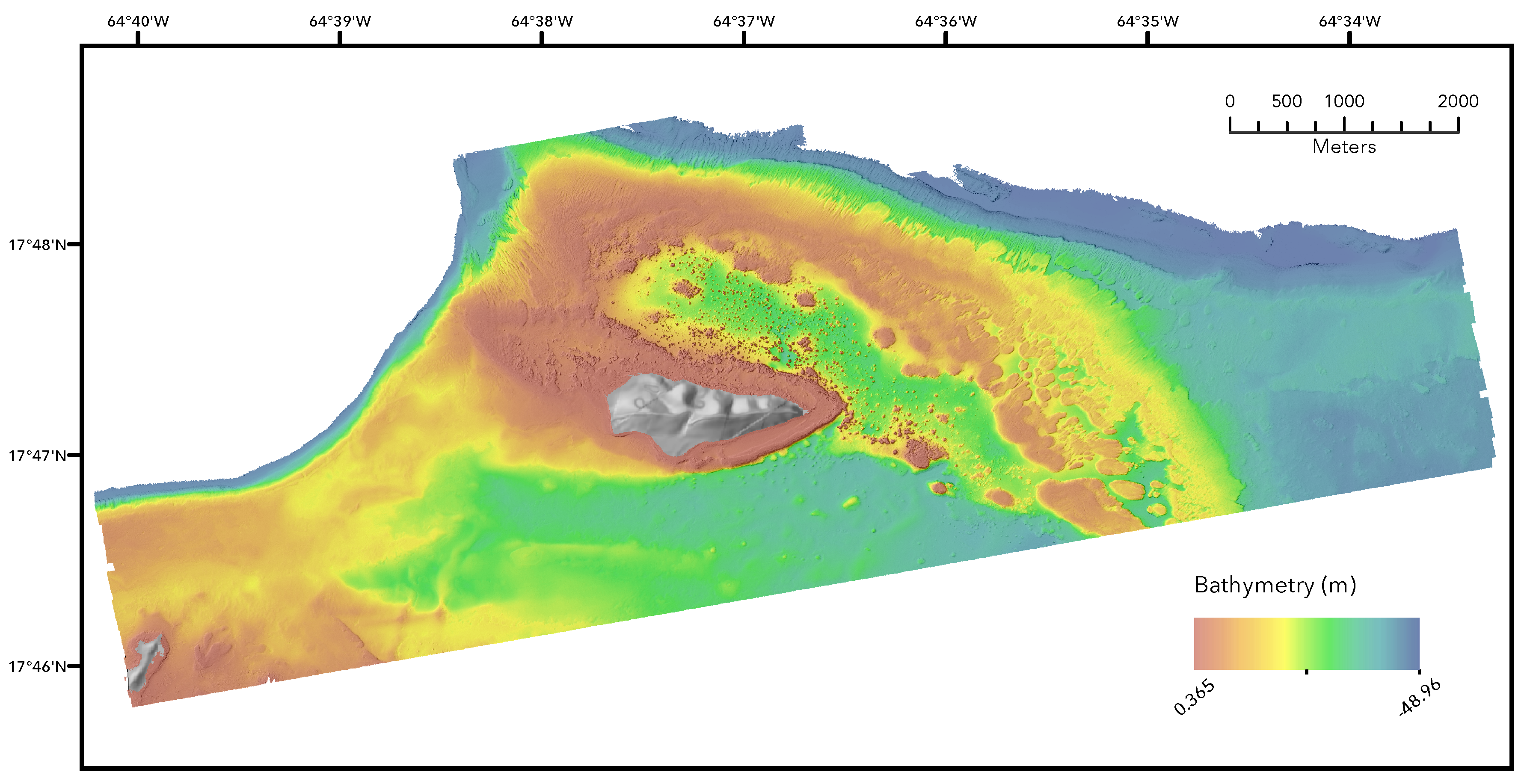
Buck Island Reef National Monument (BIRNM) is a protected area northeast of Saint Croix, U.S. Virgin Islands. Established as a protected area in 1961, both it and its surrounding seascape are well documented; the site has had extensive study of its ecology by NOAA scientists [36,60,61]. Here, our focus is not on producing a specific new map for a location, but to highlight the analytical workflows possible using BTM and its allied tools, and Buck Island provides an excellent testing ground. The reef area has extensive coverage of both MBES and LiDAR (including reflectance values), which we use for our analysis. We restricted our efforts to the LiDAR covered shallow depth locations (depth ), which include an additional LiDAR reflectance product that can be used in other packages to derive additional terrain attributes [62], here used in our covariate comparison.
Few studies of marine geomorphometry provide the data they analyzed, hampering reproducibility and standardized testing datasets that can be used across multiple studies. Buck Island was selected in part because of its full availability of datasets used, which are hosted by NOAA [63]. Additionally, the BTM generated covariates used in the analysis are also available [64]. Broader sharing of marine geomorphometry data will help this nascent field continue to grow, and benefit analytical approaches which require looking beyond individual datasets.
A breadth of literature covers in-depth analysis techniques for habitat mapping, often building up sophisticated statistical models using machine learning techniques like random forest classification [45,65]. This literature is valuable, and illuminates in-depth a single study system with the best available data and models to maximize understanding of the location and its broader modeling implications. For this work, we have targeted the common prerequisites to such a task: the production of a bethic zone mapping and interpretation of a compelling set of covariates derived from bathymetry of the generated covariates. BTM can solve both of these problems directly, and with minor additional work in R, the analytical workflow can be adopted with minimal effort. Demonstrating this workflow, and how it fits into a broader analytical task is the primary goal.
3. Results
3.1. Classified Benthnic Zone Mapping
Since its initial release, BTM has supported the generation of seafloor classification maps using only a bathymetric surface and a classification dictionary. Traditionally, the bathymetric surface was used to generate two grids of BPI (at two different scales) and a grid of slope prior to feeding these intermediate artifacts into the Classify Benthic Terrain tool, in which a classification dictionary was manually created to generate a map of benthic zones for the study area, or stored as XML. The newest release of BTM includes the Run All Model Steps tool, which condenses this workflow into a single step, and accepts both CSV and Excel files as classification dictionaries.
To demonstrate BTM’s classification mapping capabilities, a subset of the LiDAR bathymetry dataset shown in Figure 7 was classified using the Run All Model Steps tool. The original dataset was clipped to obtain a smaller study area that highlights the benthic structures immediately surrounding Buck Island.
Typical users of BTM should carefully build a unique classification dictionary for each study area by considering the context of the input data and the goals of the analysis. For each benthic zone or habitat in the table, upper and lower bounds of broad scale BPI, fine scale BPI, slope, and depth should be chosen by considering some or all of the following:
- Scale and resolution of the input data
- Scale of focal operations used to calculate BPI and slope
- Previous studies of the area of interest
- Typical values observed for the benthic zone of interest
- The range of values in each classification artifact
There is no universally applicable approach to creating a classification dictionary for use in BTM. In each case, users will need to utilize a different combination of the above resources in conjunction with professional judgment and perhaps an iterative refinement of the values used. A more rigorous approach can be obtained by using a generalized linear model (GLM) to extract the key variables as in Dunn et al. [15].
However, the purpose of this example is not to provide an accurate mapping of benthic zones in BINMR, but rather to demonstrate the typical steps that would be taken within BTM to accomplish that goal. In that context, the classification dictionary shown in Table 3 was created with an alternative approach to that recommended above.
Two BPI grids (broad and fine scale) and a slope grid were created using the clipped bathymetry dataset and the parameters listed in Table 4. Each grid was then overlayed with polygon features, each representing a benthic zone described in a 2012 benthic habitat map of the study area produced by the NOAA/NOS/NCCOS/CCMA Biogeography Branch [61]. Using the Zonal Statistics as Table tool provided with ArcGIS, the maximum and minimum values of each grid within each polygon were summarized into the classification dictionary and then revised. This method is only relevant for creating a classification dictionary to demonstrate software functionality and should not be used otherwise.
3.2. Integrating R Statistical Analysis
The ease of calculating BTM covariates is further enhanced by the ability to utilize them in predictive models or other analyses. The direct link between ArcGIS and the statistical programming language R, allows for the direct transfer of data to either software and the result of which is ready for immediate use. This functionality enables the creation of maps, the aggregation and wrangling of data, the calculation of covariates, the examination of the relationships between covariates, the building of predictive models, the analysis of diagnostic measures and charts, and more. Ultimately, the bridge enables the ability to utilize the needed tools or functions to answer the questions at hand and to create efficient and reproducible workflows. To demonstrate this, the bridge will be used to transfer BTM data to R to consider a dimensionality reduction method and to analyze the results.
After all desired BTM covariates have been derived, simultaneously working in ArcGIS and R with the same data is possible using the R-ArcGIS bridge [66]. The R-ArcGIS bridge consists of the R package, arcgisbinding, which provides functions for reading, writing, converting, and manipulating spatial data between ArcGIS and R. The advantages of the arcgisbinding package compared to packages like rgdal are most noticeable when considering the breath of data that can be transferred and when coordinated data manipulation is needed. For example, the package can read and write to any data source that exists within ArcGIS. This includes vector data stored in formats such as shapefiles, file geodatabase, or a URL for a feature service, and any supported raster data types, including complex types like mosaic datasets. Additionally, in the arcgisbinding package, the same functions used to read in data, can also be used to perform actions like creating custom subsets and selections, reprojecting both vector and raster data on the fly, and resampling and adjusting the extent of raster data. All of the above mentioned functionality is contained in the functions arc.open or arc.select if working with vector data, as shown, or arc.open and arc.raster if working with raster data.
# Load library containing R-ArcGIS bridge functionality library(arcgisbinding) # Check connection between R and ArcGIS has been established arc.check_product() input_gdb <- “C:/ArcGIS/Projects/BTM/BTM.gdb” feature_class <- “Field_AAData_ClassifiedLocations” # Establish pointer to desired data’s stored location arc_locations <- arc.open(file.path(input_gdb, feature_class)) # Convert from an ArcGIS data type to an R data frame object df_locations <- arc.select(arc_locations) # Convert from an R data frame object to a spatial data frame object # from the R package sp spdf_locations <- arc.data2sp(df_locations) |
Once this data is in its desired format, any of the functions or packages in R can be used. For example, since covariates typically used in Benthic Terrain Modeling are highly correlated, extracting the linear components of each predictor to alleviate multicollinearity prior to modeling, might be of interest. Principal component analysis is one such method for accomplishing this, by quantifying how much variance is explained by each covariate, but also by providing a useful metric for dimension reduction and building predictive models.
# Remove NAs df_locations <- na.omit(df_locations) # Creation of training/testing datasets smp_size <- floor(0.80 * nrow(df_locations)) # Randomly select observation numbers to ensure sample is randomly selected train_ind <- sample(seq_len(nrow(df_locations)), size = smp_size) # Subset the original data based on the randomly selected observation # numbers to make the training data set df_locations_train <- df_locations[train_ind, ] # Subset the original data on the remaining observations to make the # testing data set df_locations_test <- df_locations[-train_ind, ] # Make predictor variable into a factor df_locations_train$D_STRUCT <- as.factor(df_locations_train$D_STRUCT) # Separate response from the covariates btm.train_covariates <- df_locations_train[, 2:17] btm.train_response <- df_locations_train[, 1] # Apply Principal Component Analysis btm.train_pca <- prcomp(btm.train_covariates, center = TRUE, scale. = TRUE) |
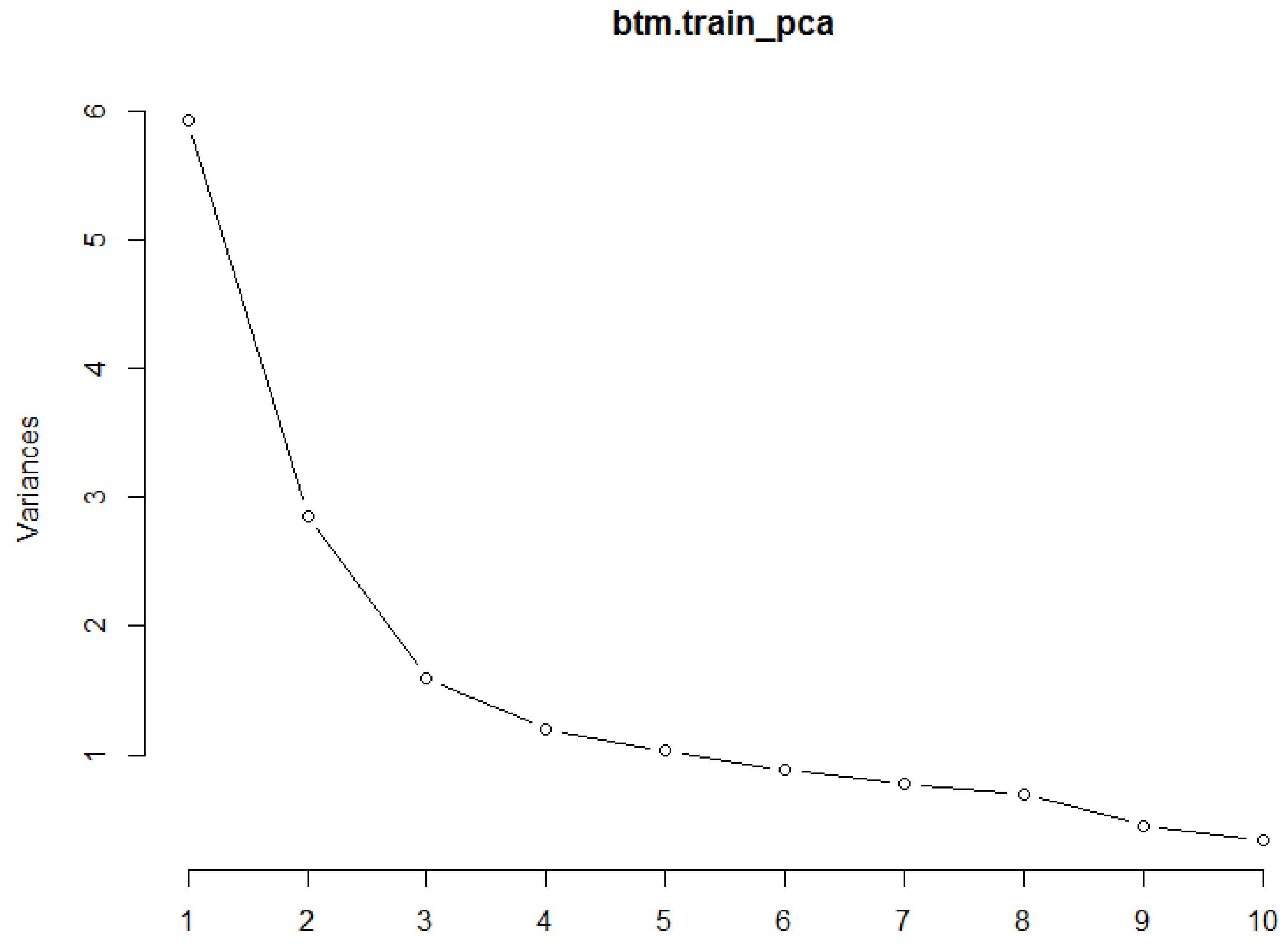
Results of the PCA analysis can be explored using functions like summary() (Figure 9) and plot() (Figure 10) to determine the proportion of variance explained by each component and which components together are able to explain up to 95 percent of the variance. From this point, results could be used to determine the most influential covariates which could then be used to construct a predictive model and assess model fit.
This example is just one possibility of the functionality between R and ArcGIS. The ease of transferring data back and forth, with the ability to perform a variety of statistical and spatial analyses, coupled with the creation of new covariates and maps allows for in depth exploration of the statistics and the science. Final results can be converted back to ArcGIS data types for the production of final maps or tables and R functionality plots can be integrated into the software through the creation of script tools and models further integrating the two.
3.3. Terrain Attribute Relationships
3.3.1. Slope
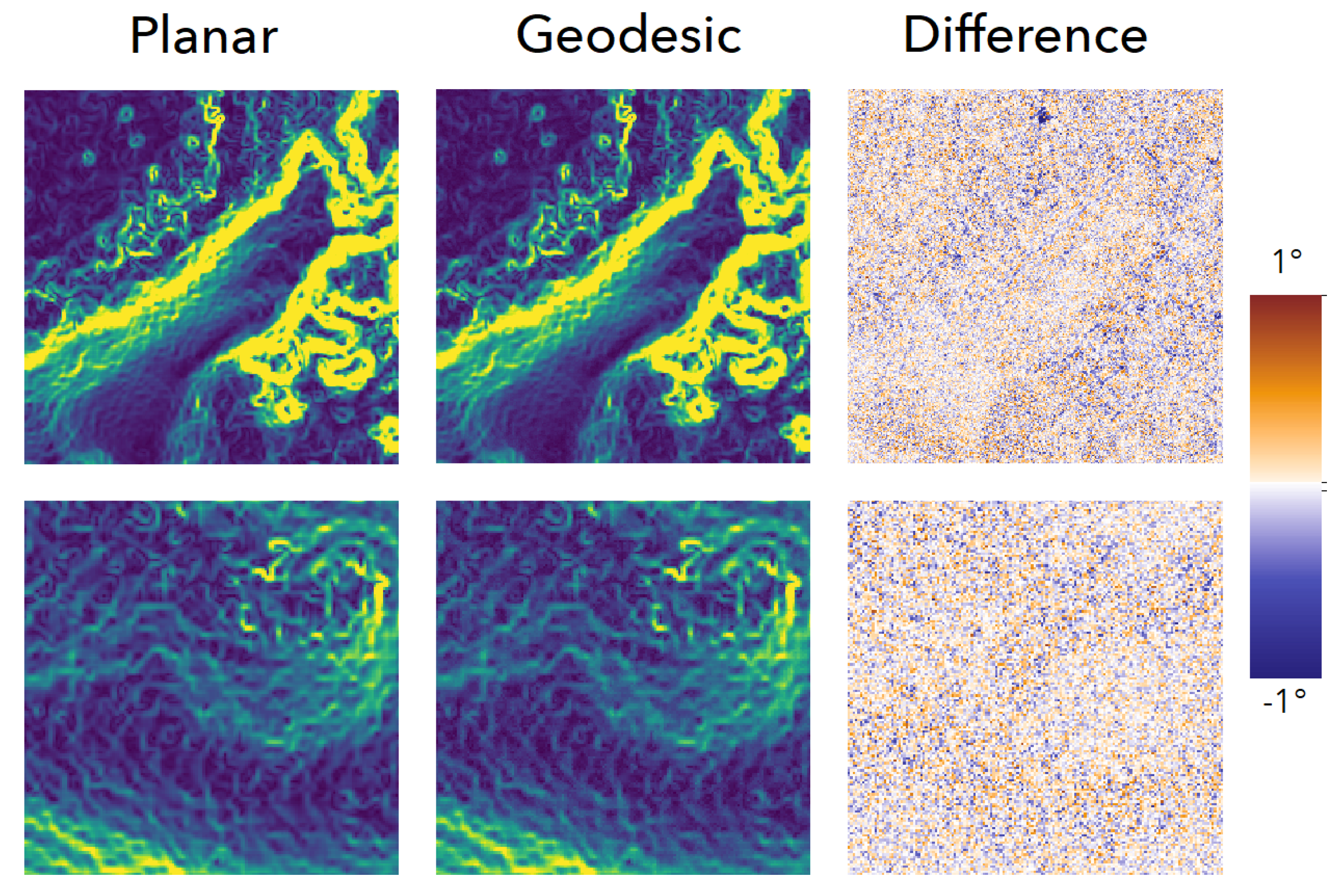
We compared Slope differences between the traditional planar form and its new geodesic variant for our example site. In most locations, little variation is seen. High rugosity areas show more marked variation, with valleys between peaks showing the biggest declines, and the edges of steep peaks showing the greatest increases (see Figure 11, Difference pane). Over the full raster, the two layers are highly correlated (Pearson correlation ). Because of this high correlation, we only relied on planar slope in our broader comparison between covariates.
3.3.2. Covariate Selection
For this study, a set of 16 covariates was selected (Table A1, [64]). Following the ordering of Section 2.1, we used BTM to generate three surface gradients (slope, aspect eastnerness, and aspect northness), four measures of relative position (broad and fine scale BPI, and slope of the slope, relative difference to the mean), three measures of surface roughness (2D ACR, VRM and SAPA), and four distribution moments (mean, standard deviation, inner-quartile range and kurtosis), with only sampling the derivatives of the multiscale algorithms. The final two covariates are the bathymetry itself, and the reflectance data from the LiDAR returns. In typical applications, the multiscaling algorithms would also be used, to measure the effect of scale on the properties, or to generate a broad suite of covariates to be used in a data reduction algorithm to select the key variables and scales.
Removing colinearity is an important step for many applications of geomorphometry [56], but is missing in most analyses, where frequently derivatives of a single DTM are used without examining the covariation that should be expected when deriving many outputs from a single input. This could be addressed within geomophometry packages, but it is a complex topic that currently resists generalization. Here, we examined the relationships between the layers (Table A2), to illustrate the importance of this step when using tools like BTM, and to examine some relationships between multiple algorithms claiming to capture similar features of DTMs. While this is limited to a single dataset, it provides some insight into some relationships between covariates that marine geomorphological tools produce.
Rugosity, and its relationship to slope, have received attention with multiple algorithms working to decouple the two [22,24]. BTM features two such rugosity algorithms, ACR (or slope-corrected SAPA) and VRM. In our study site, ACR and VRM are very strongly correlated (Pearson: 0.89), and both only moderately correlated with SAPA. In turn, SAPA shows a high correlation to slope, the standard deviation over a window, and the interquartile range. In practice, standard deviation and the interquartile range are less correlated over larger neighborhoods, but the strong correlation between SAPA and slope shows the limited utility of SAPA as an independent measurement in models which already contain slope as a covariate.
A measure suggested by Lecours et al. [56] based on his evaluation of over 200 covariates is relative difference from mean depth (the value minus the mean divided by the range). With our data this measure showed no meaningful correlations, providing a useful addition. Similarly, Pittman et al. [65] and others have recommended “slope of the slope”, executing the slope function a second time on the slope raster, and again we show little correlation with this result to others in the covariates we analyzed, though the term “slope of the slope” can be methodologically confusing because of its conceptual overlap with curvature. Finally, kurtosis showed no meaningful correlations and should be examined as another potentially useful derivative.
3.3.3. Remarks
Here we have shown the basic workflow of using BTM to create benthic zone classifications, to use BTM to create a collection of covariates for later use and interpretation, and how to extend the workflow using R. In practice, BTM is used in all these roles. It may be used to create simple slope and rugosity layers, as was done in McNeil et al. [67]. The software can also be used to generate covariates at multiple scales to aid in understanding the effects of scale on prediction models like Maximum Entropy (MaxEnt) model outputs as in Miyamoto et al. [68]. In use cases like Li et al. [69], the outputs from BTM are used in an unsupervised classification using the ISODATA algorithm to build a validated benthic classification map. While BTM has been providing new algorithms for rugosity for many years, it is still common for users to rely on earlier methods like SAPA [70], likely because of its well-known association with capturing rugosity. It will take time, and a greater exposure of the benefits of slope-decoupled roughness for this to change. More studies which explicitly examine a large gamut of covariates like [56] are needed to improve our understanding of the relationships between the derived covariates, which usually ultimately derive from a single input dataset.
4. Discussion
The analysis shows how BTM can be used to produce semi-automated classifications of locations, using easy to use tools, and how to incorporate BTM and the terrain attributes it produces into a larger analysis context. This case study is intended to be simple with reproducible data, and the authors hope that reuse of publicly available well documented datasets will become more common in the community to facilitate collaboration. An accessible but powerful analysis framework is available by combining BTM and ArcGIS with the broader scientific software ecosystem in Python and R. As marine geomorphology matures as a discipline, adapting to rich and accessible tools provides a key way for both students and researchers to perform rigorous analysis. BTM has grown in part to adapt to these needs, and we illustrate some of the new approaches it has incorporated to help with this process.
While improvements accumulate, there remain gaps in the analytical tools available that deserve deeper investment. Implementations measuring fractal dimension [71] remain rare, and could be aided by being more broadly accessible. Multiscale analysis, while partially captured in BTM and other tools, could be greatly improved by the incorporation of characteristic scales [72] to formalize understanding on the role of scale. Instead of relying on cell-based analysis and resampling, object-based models provide a better potential basic unit for analysis [73]. Similarly, the data capture process primarily observes point based observations, and analyzing these directly provides another avenue forward [74]. Terrestrial geomorphology still enjoys advantages in consistent global datasets which form a common benchmark for analysis, but as the process for capturing and processing marine data continue to improve, this goal should also be attainable in the marine domain. Continued improvements in the marine geomorphology research community will be well served with broadly available and well understood tools available for researchers, and we hope to allow BTM to continue serving in this capacity.
Acknowledgments
Institutional support provided by: Esri, NOAA Costal Service Center, Massachusetts Office of Coastal Zone Management, and Oregon State University. Thanks to Cherisse Du Preez, Matt Pendleton, Jen Boulware, Lisa Wedding, Pat Iampietro and Ellen Hines for their contributions. Thanks to our anonymous reviewers, they have greatly improved the text.
Author Contributions
N.S. and S.W. conceived and designed the analysis; N.S., M.P. and S.W. performed the analysis; N.S., M.P. and S.W. analyzed the data; D.W., N.S., M.P. and S.W. wrote the paper.
Conflicts of Interest
The authors declare no conflict of interest.
Abbreviations
The following abbreviations are used in this manuscript:
| AOI | Area of interest |
| BIRNM | Buck Island Reef National Monument |
| BPI | Bathymetric Position Index |
| BTM | Benthic Terrain Modeler |
| DTM | Digital terrain model |
| GIS | Geographic information system |
| IQR | Interquartile range |
| LiDAR | Light Detection and Ranging |
| MBES | Multibeam Ecosounder |
| NOAA | National Oceanic and Atmospheric Administration |
| POBF | Plane of best fit |
| SAPA | Surface area to planar area |
| TIN | Triangulated irregular network |
| VRM | Vector ruggedness measure |
Appendix A.
Appendix A.1. Derived Parameters
Covariance is defined as:
where
- k denotes the position of the current raster cell;
- Z is the value of the cell;
- i and j are the two rasters being compared;
- is the mean of the raster;
- N is the total number of cells.
The Pearson correlation coefficient between rasters i and j is:
where is the standard deviation of rasters i and j.

Table A1.
Mapping of the environmental covariates to their layer names.
| Layer | Environmental Covariate |
|---|---|
| 1 | Aspect easterness |
| 2 | Aspect northerness |
| 3 | Broad scale BPI standardized (60–80) |
| 4 | Fine scale BPI standardized (10–15) |
| 5 | Interquartile range (IQR) |
| 6 | Bathymetry (LiDAR) |
| 7 | Kurtosis (Pearson) |
| 8 | Mean |
| 9 | Relative difference to mean |
| 10 | Standard deviation |
| 11 | Reflectance (LiDAR) |
| 12 | Slope (planar) |
| 13 | Slope of the slope (max in slope) |
| 14 | Rugosity (ACR) |
| 15 | Rugosity (SAPA) |
| 16 | Rugosity (VRM) |
Table A2.
Upper triangle is pairwise covariance, lower triangle is pairwise correlation. Pearson correlation coefficients bold for very strong correlations, italic for strong correlations [75], layer labels in Table A1.
| Layer | 1 | 2 | 3 | 4 | 5 | 6 | 7 | 8 | 9 | 10 | 11 | 12 | 13 | 14 | 15 | 16 |
|---|---|---|---|---|---|---|---|---|---|---|---|---|---|---|---|---|
| 1 | −0.001505 | −0.000064 | −0.000070 | −0.000074 | −0.001187 | −0.000116 | −0.001187 | −0.000151 | −0.000113 | 0.000753 | −0.000293 | −0.001150 | −0.000004 | −0.000014 | −0.000005 | |
| 2 | −0.02035 | −0.000174 | −0.000018 | 0.000274 | −0.005216 | −0.000269 | −0.005231 | 0.000012 | 0.000360 | 0.002170 | 0.000938 | 0.003334 | 0.000013 | 0.000045 | 0.000013 | |
| 3 | −0.00781 | −0.02005 | 0.000123 | 0.000072 | 0.000495 | −0.000025 | 0.000460 | 0.000110 | 0.000102 | −0.000443 | 0.000236 | 0.000704 | 0.000010 | 0.000036 | 0.000022 | |
| 4 | −0.01952 | −0.00471 | 0.29382 | 0.000070 | −0.000161 | −0.000008 | −0.000159 | 0.000063 | 0.000099 | −0.000181 | 0.000223 | 0.000489 | 0.000016 | 0.000040 | 0.000031 | |
| 5 | −0.02094 | 0.0727 | 0.17456 | 0.38188 | −0.000080 | −0.000094 | −0.000078 | 0.000012 | 0.000235 | −0.000157 | 0.000551 | 0.001311 | 0.000020 | 0.000083 | 0.000033 | |
| 6 | −0.0371 | −0.15321 | 0.13208 | −0.09758 | −0.04917 | −0.000071 | 0.014664 | −0.000356 | −0.000091 | −0.005869 | −0.000263 | −0.001478 | −0.000001 | 0.000015 | 0.000014 | |
| 7 | −0.01123 | −0.02448 | −0.02069 | −0.0156 | −0.17901 | −0.01488 | −0.000068 | −0.000030 | −0.000077 | −0.000073 | −0.000219 | 0.000277 | 0.000003 | −0.000013 | 0.000002 | |
| 8 | −0.03705 | −0.15354 | 0.12279 | −0.09619 | −0.0476 | 0.99459 | −0.0142 | −0.000357 | −0.000091 | −0.005891 | −0.000261 | −0.001482 | −0.000001 | 0.000015 | 0.000014 | |
| 9 | −0.01078 | 0.00082 | 0.06726 | 0.0872 | 0.01686 | −0.05514 | −0.01445 | −0.05526 | 0.000016 | −0.000172 | 0.000040 | −0.000146 | 0.000002 | 0.000005 | 0.000004 | |
| 10 | −0.02384 | 0.07124 | 0.18349 | 0.40352 | 0.96982 | −0.0415 | −0.10875 | −0.04173 | 0.01651 | −0.000540 | −0.002241 | −0.000031 | −0.000086 | −0.000055 | 0.000048 | |
| 11 | 0.03378 | 0.0915 | −0.16976 | −0.15727 | −0.13822 | −0.57182 | −0.02204 | −0.57346 | −0.0384 | −0.15457 | −0.000540 | −0.002241 | −0.000031 | −0.000086 | −0.000055 | |
| 12 | −0.02606 | 0.0785 | 0.17926 | 0.38571 | 0.96182 | −0.05086 | −0.1308 | −0.0505 | 0.01777 | 0.99042 | −0.14996 | 0.004609 | 0.000066 | 0.000245 | 0.000106 | |
| 13 | −0.02568 | 0.06997 | 0.13414 | 0.21164 | 0.57397 | −0.07169 | 0.04158 | −0.0718 | −0.0162 | 0.61259 | −0.15597 | 0.63653 | 0.000182 | 0.000415 | 0.000301 | |
| 14 | −0.0055 | 0.01546 | 0.10146 | 0.38474 | 0.48963 | −0.00152 | 0.02906 | −0.00171 | 0.00986 | 0.54408 | −0.11896 | 0.50955 | 0.35024 | 0.000012 | 0.000013 | |
| 15 | −0.00734 | 0.02177 | 0.16034 | 0.40183 | 0.83457 | 0.01642 | −0.04372 | 0.01634 | 0.01338 | 0.85408 | −0.13833 | 0.78137 | 0.33215 | 0.54067 | 0.000020 | |
| 16 | −0.00395 | 0.0102 | 0.15266 | 0.48178 | 0.51791 | 0.02527 | 0.0124 | 0.02513 | 0.01487 | 0.5628 | −0.13889 | 0.52841 | 0.37625 | 0.89434 | 0.5639 |
References
- Halpern, B.S.; Walbridge, S.; Selkoe, K.A.; Kappel, C.V.; Micheli, F.; D’Agrosa, C.; Bruno, J.F.; Casey, K.S.; Ebert, C.; Fox, H.E.; et al. A global map of human impact on marine ecosystems. Science 2008, 319, 948–952. [Google Scholar] [CrossRef] [PubMed]
- Wright, D.J.; Heyman, W.D. Introduction to the Special Issue: Marine and Coastal GIS for Geomorphology, Habitat Mapping, and Marine Reserves. Mar. Geodesy 2008, 31, 1–8. [Google Scholar] [CrossRef]
- Becker, J.J.; Sandwell, D.T.; Smith, W.H.; Braud, J.; Binder, B.; Depner, J.; Fabre, D.; Factor, J.; Ingalls, S.; Kim, S.H.; et al. Global Bathymetry and Elevation Data at 30 Arc Seconds Resolution: SRTM30_PLUS. Mar. Geodesy 2009, 32, 355–371. [Google Scholar] [CrossRef]
- Sayre, R.; Wright, D.; Aniello, P.; Breyer, S.; Cribbs, D.; Frye, C.; Vaughan, R.; Van Esch, B.; Stephens, D.; Harris, P.; et al. Mapping EMUs (Ecological Marine Units)–the creation of a global GIS of distinct marine environments to support marine spatial planning, management and conservation. In Proceedings of the Fifteenth International Symposium of Marine Geological and Biological Habitat Mapping (GEOHAB 2015), Bahia, Brazil, 1–8 May 2015; p. 21. [Google Scholar]
- Pittman, S.J. Seascape Ecology; John Wiley & Sons: Hoboken, NJ, USA, 2017. [Google Scholar]
- Brock, J.C.; Wright, C.W.; Clayton, T.D.; Nayegandhi, A. LIDAR optical rugosity of coral reefs in Biscayne National Park, Florida. Coral Reefs 2004, 23, 48–59. [Google Scholar] [CrossRef]
- García-Alegre, A.; Sánchez, F.; Gómez-Ballesteros, M.; Hinz, H.; Serrano, A.; Parra, S. Modelling and mapping the local distribution of representative species on the Le Danois Bank, El Cachucho Marine Protected Area (Cantabrian Sea). In Deep-Sea Research Part II: Topical Studies in Oceanography; Elsevier: Amsterdam, The Netherlands, 2014; Volume 106, pp. 151–164. [Google Scholar]
- Brown, C.J.; Smith, S.J.; Lawton, P.; Anderson, J.T. Benthic habitat mapping: A review of progress towards improved understanding of the spatial ecology of the seafloor using acoustic techniques. Estuar. Coast. Shelf Sci. 2011, 92, 502–520. [Google Scholar] [CrossRef]
- Bishop, M.P.; James, L.A.; Shroder, J.F.; Walsh, S.J. Geospatial technologies and digital geomorphological mapping: Concepts, issues and research. Geomorphology 2012, 137, 5–26. [Google Scholar] [CrossRef]
- Passalacqua, P.; Belmont, P.; Staley, D.M.; Simley, J.D.; Arrowsmith, J.R.; Bode, C.A.; Crosby, C.; DeLong, S.B.; Glenn, N.F.; Kelly, S.A.; et al. Analyzing high resolution topography for advancing the understanding of mass and energy transfer through landscapes: A review. Earth-Sci. Rev. 2015, 148, 174–193. [Google Scholar] [CrossRef] [Green Version]
- Lecours, V.; Dolan, M.F.; Micallef, A.; Lucieer, V.L. A review of marine geomorphometry, the quantitative study of the seafloor. Hydrol. Earth Syst. Sci. 2016, 20, 3207–3244. [Google Scholar] [CrossRef]
- Lundblad, E.R.; Wright, D.J.; Miller, J.; Larkin, E.M.; Rinehart, R.; Naar, D.F.; Donahue, B.T.; Anderson, S.M.; Battista, T. A Benthic Terrain Classification Scheme for American Samoa. Mar. Geodesy 2006, 29, 89–111. [Google Scholar] [CrossRef]
- Wright, D.; Pendleton, M.; Boulware, J.; Walbridge, S.; Gerlt, B.; Eslinger, D.; Sampson, D.; Huntley, E. ArcGIS Benthic Terrain Modeler (BTM), v. 3.0, Environmental Systems Research Institute, NOAA Coastal Services Center, Massachusetts Office of Coastal Zone Management. Available online: https://esriurl.com/5754 (accessed on 27 February 2018).
- Young, M.; Ierodiaconou, D.; Womersley, T. Forests of the sea: Predictive habitat modelling to assess the abundance of canopy forming kelp forests on temperate reefs. Remote Sens. Environ. 2015, 170, 178–187. [Google Scholar] [CrossRef]
- Dunn, D.; Halpin, P. Rugosity-based regional modeling of hard-bottom habitat. Mar. Ecol. Prog. Ser. 2009, 377, 1–11. [Google Scholar] [CrossRef]
- Verfaillie, E.; Degraer, S.; Schelfaut, K.; Willems, W.; Van Lancker, V. A protocol for classifying ecologically relevant marine zones, a statistical approach. Estuar. Coast. Shelf Sci. 2009, 83, 175–185. [Google Scholar] [CrossRef]
- Diesing, M.; Coggan, R.; Vanstaen, K. Widespread rocky reef occurrence in the central English Channel and the implications for predictive habitat mapping. Estuar. Coast. Shelf Sci. 2009, 83, 647–658. [Google Scholar] [CrossRef]
- Horn, B.K. Hill shading and the reflectance map. Proc. IEEE 1981, 69, 14–47. [Google Scholar] [CrossRef]
- Olaya, V. Basic land-surface parameters. Geomorphometry Concepts Softw. Appl. 2009, 33, 141–169. [Google Scholar]
- Florinsky, I.V. An illustrated introduction to general geomorphometry. Prog. Phys. Geogr. 2017, 41, 723–752. [Google Scholar] [CrossRef]
- Zwillinger, D.; Kokoska, S. CRC Standard Probability and Statistics Tables and Formulae; CRC Press: Boca Raton, FL, USA, 1999. [Google Scholar]
- Sappington, J.M.; Longshore, K.M.; Thompson, D.B. Quantifying Landscape Ruggedness for Animal Habitat Analysis: A Case Study Using Bighorn Sheep in the Mojave Desert. J. Wildl. Manag. 2007, 71, 1419–1426. [Google Scholar] [CrossRef]
- Jenness, J.S. Calculating landscape surface area from digital elevation models. Wildl. Soc. Bull. 2004, 32, 829–839. [Google Scholar] [CrossRef]
- Du Preez, C. A new arc–chord ratio (ACR) rugosity index for quantifying three-dimensional landscape structural complexity. Landsc. Ecol. 2015, 30, 181–192. [Google Scholar] [CrossRef]
- Weisstein, E.W. MathWorld: Moore Neighborhood. Available online: http://mathworld.wolfram.com/MooreNeighborhood.html (accessed on 27 February 2018).
- Evans, I.S. An integrated system of terrain analysis and slope mapping. Z. fur Geomorphol. 1980, 36, 274–295. [Google Scholar]
- Wood, J. The Geomorphological Characterisation of Digital Elevation Models. PhD Thesis, University of Leicester, Leicester, UK, 1996. [Google Scholar]
- Rigol-Sanchez, J.P.; Stuart, N.; Pulido-Bosch, A. ArcGeomorphometry: A toolbox for geomorphometric characterisation of DEMs in the ArcGIS environment. Comput. Geosci. 2015, 85, 155–163. [Google Scholar] [CrossRef]
- Dolan, M.F.; Lucieer, V.L. Variation and Uncertainty in Bathymetric Slope Calculations Using Geographic Information Systems. Mar. Geodesy 2014, 37, 187–219. [Google Scholar] [CrossRef]
- Ligas, M.; Banasik, P. Conversion between Cartesian and geodetic coordinates on a rotational ellipsoid by solving a system of nonlinear equations. Geodesy Cartogr. 2011, 60, 145–159. [Google Scholar] [CrossRef]
- Lecours, V.; Devillers, R.; Simms, A.E.; Lucieer, V.L.; Brown, C.J. Towards a framework for terrain attribute selection in environmental studies. Environ. Model. Softw. 2017, 89, 19–30. [Google Scholar] [CrossRef]
- Davies, A.J.; Wisshak, M.; Orr, J.C.; Murray Roberts, J. Predicting suitable habitat for the cold-water coral Lophelia pertusa (Scleractinia). In Deep-Sea Research Part I: Oceanographic Research Papers; Elsevier: Amsterdam, The Netherlands, 2008; Volume 55, pp. 1048–1062. [Google Scholar]
- Smith, N.; Van der Walt, S. A Better Default Colormap for Matplotlib. Available online: https://bids.github.io/colormap/ (accessed on 27 February 2018).
- Wilson, M.F.J.; O’Connell, B.; Brown, C.; Guinan, J.C.; Grehan, A.J. Multiscale Terrain Analysis of Multibeam Bathymetry Data for Habitat Mapping on the Continental Slope. Mar. Geodesy 2007, 30, 3–35. [Google Scholar] [CrossRef]
- Lucieer, V.; Pederson, H. Linking morphometric characterisation of rocky reef with fine scale lobster movement. ISPRS J. Photogramm. Remote Sens. 2008, 63, 496–509. [Google Scholar] [CrossRef]
- Pittman, S.J.; Hile, S.D.; Jeffrey, C.F.G.; Caldow, C.; Kendall, M.S.; Monaco, M.E.; Hillis-Starr, Z. Fish assemblages and benthic habitats of Buck Island Reef National Monument (St. Croix, U.S. Virgin Islands) and the surrounding seascape: A characterization of spatial and temporal patterns. NOAA Tech. Memo. NOS NCCOS 2008, 71, 1–80. [Google Scholar]
- Zevenbergen, L.W.; Thorne, C.R. Quantitative analysis of land surface topography. Earth Surf. Process. Landf. 1987, 12, 47–56. [Google Scholar] [CrossRef]
- Weiss, A.D. Topographic Position and Landforms Analysis. In Proceedings of the Esri User Conference, San Diego, CA, USA, 26–30 June 2000; p. 1. [Google Scholar]
- Iampietro, P.; Kvitek, R. Quantitative seafloor habitat classification using GIS terrain analysis: Effects of data density, resolution, and scale. In Proceedings of the 22nd Annual ESRI User Conference, San Diego, CA, USA, 9–13 July 2002; pp. 8–12. [Google Scholar]
- Lecours, V. On the Use of Maps and Models in Conservation and Resource Management (Warning: Results May Vary). Front. Mar. Sci. 2017, 4, 1–18. [Google Scholar] [CrossRef]
- Riley, S.; Degloria, S.; Elliot, S. A Terrain Ruggedness Index that Quantifies Topographic Heterogeneity. Int. J. Sci. 1999, 5, 23–27. [Google Scholar]
- Friedman, A.; Pizarro, O.; Williams, S.B.; Johnson-Roberson, M. Multi-Scale Measures of Rugosity, Slope and Aspect from Benthic Stereo Image Reconstructions. PLoS ONE 2012, 7. [Google Scholar] [CrossRef] [PubMed]
- Hobson, R. Surface roughness in topography: Quantitative approach. In Spatial Analysis in Geomorphology; Methuen: London, UK, 1972; pp. 221–245. [Google Scholar]
- Du Preez, C.; Curtis, J.M.; Clarke, M.E. The structure and distribution of benthic communities on a shallow seamount (Cobb Seamount, Northeast Pacific Ocean). PLoS ONE 2016, 11, e0165513. [Google Scholar] [CrossRef] [PubMed]
- Wedding, L.M.; Friedlander, A.M.; McGranaghan, M.; Yost, R.S.; Monaco, M.E. Using bathymetric lidar to define nearshore benthic habitat complexity: Implications for management of reef fish assemblages in Hawaii. Remote Sens. Environ. 2008, 112, 4159–4165. [Google Scholar] [CrossRef]
- Grohmann, C.H.; Smith, M.J.; Riccomini, C. Multiscale analysis of topographic surface roughness in the Midland Valley, Scotland. IEEE Trans. Geosci. Remote Sens. 2011, 49, 1200–1213. [Google Scholar] [CrossRef]
- Jones, E.; Oliphant, T.; Peterson, P. SciPy: Open Source Scientific Tools For Python. Available online: http://www.scipy.org/ (accessed on 10 January 2018).
- DeCarlo, L.T. On the meaning and use of kurtosis. Psychol. Methods 1997, 2, 292. [Google Scholar] [CrossRef]
- Bartels, M.; Wei, H.; Mason, D.C. DTM generation from LIDAR data using skewness balancing. In Proceedings of the 18th IEEE International Conference on Pattern Recognition, Hong Kong, China, 20–24 August 2006; Volume 1, pp. 566–569. [Google Scholar]
- Mark, D.M. Geomorphometric parameters: A review and evaluation. Geogr. Ann. Ser. A Phys. Geogr. 1975, 165–177. [Google Scholar] [CrossRef]
- Hey, T.; Tansley, S.; Tolle, K. The Fourth Paradigm: Data-Intensive Scientific Discovery; Microsoft Research: Washington, DC, USA, 2009. [Google Scholar]
- Guo, P. Python Is Now the Most Popular Introductory Teaching Language at Top U.S. Universities. Available online: https://cacm.acm.org/blogs/blog-cacm/176450 (accessed on 27 February 2018).
- Walbridge, S.; Slocum, N. GitHub: Benthic Terrain Modeler. Available online: https://github.com/EsriOceans/btm (accessed on 27 February 2018).
- Conrad, O.; Bechtel, B.; Bock, M.; Dietrich, H.; Fischer, E.; Gerlitz, L.; Wehberg, J.; Wichmann, V.; Böhner, J. System for automated geoscientific analyses (SAGA) v. 2.1.4. Geosci. Model Dev. 2015, 8, 1991–2007. [Google Scholar] [CrossRef]
- Neteler, M.; Bowman, M.; Landa, M.; Metz, M. GRASS GIS: A multi-purpose Open Source GIS. Environ. Model. Softw. 2012, 31, 124–130. [Google Scholar] [CrossRef]
- Lecours, V.; Brown, C.J.; Devillers, R.; Lucieer, V.L.; Edinger, E.N. Comparing selections of environmental variables for ecological studies: A focus on terrain attributes. PLoS ONE 2016, 11, 1–18. [Google Scholar] [CrossRef] [PubMed]
- Evans, J.; Oakleaf, J.; Cushman, S. An ArcGIS Toolbox for Surface Gradient and Geomorphometric Modeling, Version 2.0-0. Available online: http://evansmurphy.wix.com/evansspatial (accessed on 3 January 2018).
- Trevisani, S.; Rocca, M. MAD: Robust image texture analysis for applications in high resolution geomorphometry. Comput. Geosci. 2015, 81, 78–92. [Google Scholar] [CrossRef]
- Roberts, J.J.; Best, B.D.; Dunn, D.C.; Treml, E.A.; Halpin, P.N. Marine Geospatial Ecology Tools: An integrated framework for ecological geoprocessing with ArcGIS, Python, R, MATLAB, and C++. Environ. Model. Softw. 2010, 25, 1197–1207. [Google Scholar] [CrossRef]
- Kendall, M.; Miller, T.; Pittman, S. Patterns of scale-dependency and the influence of map resolution on the seascape ecology of reef fish. Mar. Ecol. Prog. Ser. 2011, 427, 259–274. [Google Scholar] [CrossRef]
- Costa, B.M.; Tormey, S.; Battista, T.A. Benthic Habitats of Buck Island Reef National Monument; NOAA National Centers for Coastal Ocean Science: Silver Spring, MD, USA, 2012. [Google Scholar]
- Zavalas, R.; Ierodiaconou Daniel, D.; Ryan, D.; Rattray, A.; Monk, J. Habitat classification of temperate marine macroalgal communities using bathymetric LiDAR. Remote Sens. 2014, 6, 2154–2175. [Google Scholar] [CrossRef]
- Battista, T.; Costa, B. Buck Island Reef National Monument. Available online: https://products.coastalscience.noaa.gov/collections/benthic/e93stcroix/ (accessed on 10 January 2018).
- Walbridge, S. Buck Island, Covariate Geodatabase. Available online: https://figshare.com/articles/Buck_Island_-_Covariate_Stack/5946463 (accessed on 27 February 2018).
- Pittman, S.; Costa, B.; Battista, T. Using lidar bathymetry and boosted regression trees to predict the diversity and abundance of fish and corals. J. Coast. Res. 2009, 27–38. [Google Scholar] [CrossRef]
- Pavlushko, D.; Pobuda, M.; Walbridge, S.; Kopp, S.; Aydin, O.; Krivoruchko, K.; Janikas, M. R-ArcGIS Bridge, Environmental Systems Research Institute. Available online: https://r-arcgis.github.io (accessed on 27 February 2018).
- McNeil, M.A.; Webster, J.M.; Beaman, R.J.; Graham, T.L. New constraints on the spatial distribution and morphology of the Halimeda bioherms of the Great Barrier Reef, Australia. Coral Reefs 2016, 35, 1343–1355. [Google Scholar] [CrossRef]
- Miyamoto, M.; Kiyota, M.; Murase, H.; Nakamura, T.; Hayashibara, T. Effects of Bathymetric Grid-Cell Sizes on Habitat Suitability Analysis of Cold-water Gorgonian Corals on Seamounts. Mar. Geodesy 2017, 40, 205–223. [Google Scholar] [CrossRef]
- Li, D.; Tang, C.; Xia, C.; Zhang, H. Acoustic mapping and classification of benthic habitat using unsupervised learning in artificial reef water. Estuar. Coast. Shelf Sci. 2017, 185, 11–21. [Google Scholar] [CrossRef]
- D’Antonio, N.L.; Gilliam, D.S.; Walker, B.K. Investigating the spatial distribution and effects of nearshore topography on Acropora cervicornis abundance in Southeast Florida. PeerJ 2016, 4, e2473. [Google Scholar] [CrossRef] [PubMed]
- Mark, D.M.; Aronson, P.B. Scale-dependent fractal dimensions of topographic surfaces: An empirical investigation, with applications in geomorphology and computer mapping. J. Int. Assoc. Math. Geol. 1984, 16, 671–683. [Google Scholar] [CrossRef]
- Perron, J.T.; Kirchner, J.W.; Dietrich, W.E. Formation of evenly spaced ridges and valleys. Nature 2009, 460, 502–505. [Google Scholar] [CrossRef]
- Deng, Y.X.; Wilson, J.P. The Role of Attribute Selection in GIS Representations of the Biophysical Environment. Ann. Assoc. Am. Geogr. 2006, 96, 47–63. [Google Scholar] [CrossRef]
- Brasington, J.; Vericat, D.; Rychkov, I. Modeling river bed morphology, roughness, and surface sedimentology using high resolution terrestrial laser scanning. Water Resour. Res. 2012, 48. [Google Scholar] [CrossRef]
- Evans, J. Straightforward Statistics for the Behavioral Sciences; Brooks/Cole Publishing Company: Pacific Grove, CA, USA, 1996. [Google Scholar]
Figure 1.
Least squares fitting of the curvature calculations, including that used by the geodesic slope computation. The pink curve is a polynomial fit against the cells in each neighborhood, here labeled to where is the origin cell.
Figure 1.
Least squares fitting of the curvature calculations, including that used by the geodesic slope computation. The pink curve is a polynomial fit against the cells in each neighborhood, here labeled to where is the origin cell.

Figure 2.
Buck Island Reef National Monument LiDAR depth data Section 2.3, and the surface gradients of planar slope, northerness and easterness. Upper left: planar slope, displayed with the perceptually uniform color map viridis [33], in degrees, values normalized by the standard deviation (). Center left: Northerness of aspect, from due north to due south (1 to −1), linear ramp. Lower left: Easterness of aspect, from due east to due west (1 to −1), linear ramp. Inset maps: (A) is east of island, with large depth variation along a reef edge; (B) is along the bank in the northeast corner of the region.
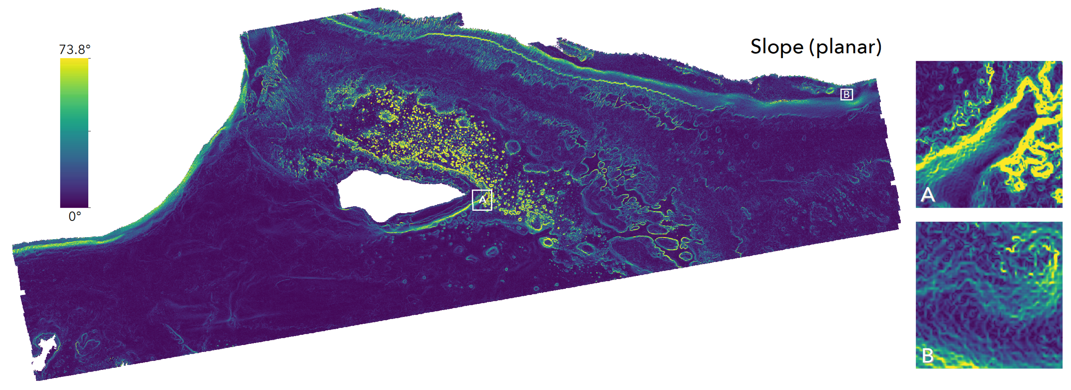

Figure 3.
The tape-chain rugosity measurement is an in-situ method of evaluating terrain heterogeneity. The ratio of the chain length () to profile length () describes the rugosity of the two dimensional profile. Used under Creative Commons Attribution license (CC BY) from Friedman et al. [42].
Figure 3.
The tape-chain rugosity measurement is an in-situ method of evaluating terrain heterogeneity. The ratio of the chain length () to profile length () describes the rugosity of the two dimensional profile. Used under Creative Commons Attribution license (CC BY) from Friedman et al. [42].

Figure 4.
Components required to calculate Arc-Chord Ratio (ACR) (a) for a bathymetric surface using a moving window, and (b) for an area of interest using a triangulated irregular network. Reprinted by permission from Cherisse Du Preez: Springer Nature Landscape Ecology, 2015 [24].
Figure 4.
Components required to calculate Arc-Chord Ratio (ACR) (a) for a bathymetric surface using a moving window, and (b) for an area of interest using a triangulated irregular network. Reprinted by permission from Cherisse Du Preez: Springer Nature Landscape Ecology, 2015 [24].

Figure 5.
Output from Compare Scales of Analysis tool, with Median calculated for focal neighborhoods ranging from to . Fine scale detail is lost by the neighborhood, and only broad trends remain at the scale.
Figure 5.
Output from Compare Scales of Analysis tool, with Median calculated for focal neighborhoods ranging from to . Fine scale detail is lost by the neighborhood, and only broad trends remain at the scale.
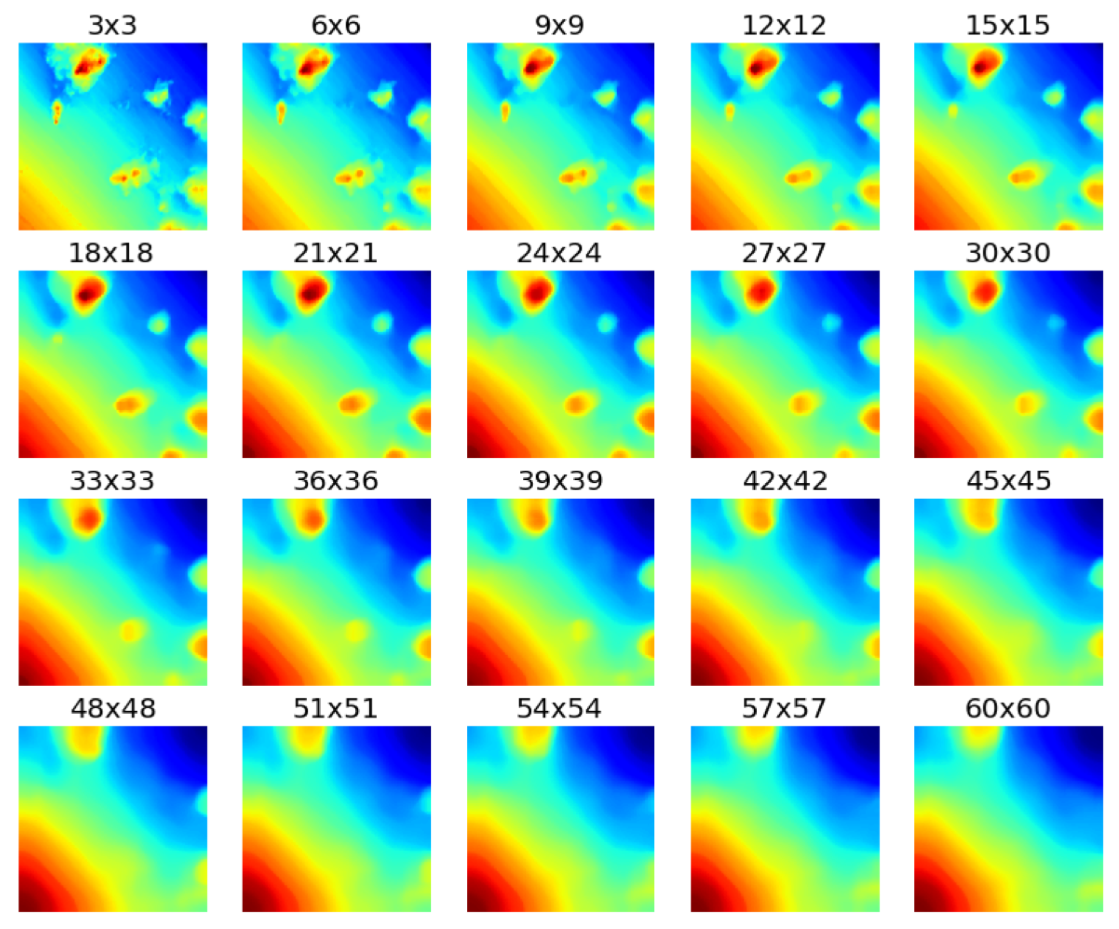
Figure 6.
The BTM Python Add-in, which provides a simple graphical interface for accessing the analytical tools provided.
Figure 6.
The BTM Python Add-in, which provides a simple graphical interface for accessing the analytical tools provided.

Figure 7.
Buck Island National Marine Reserve LiDAR bathymetry (3 m resolution) coverage.

Figure 8.
A habitat classification map created for a subregion of Buck Island National Marine Reserve using the Run All Model Steps tool. The white zone represents terrain above sea level.
Figure 8.
A habitat classification map created for a subregion of Buck Island National Marine Reserve using the Run All Model Steps tool. The white zone represents terrain above sea level.
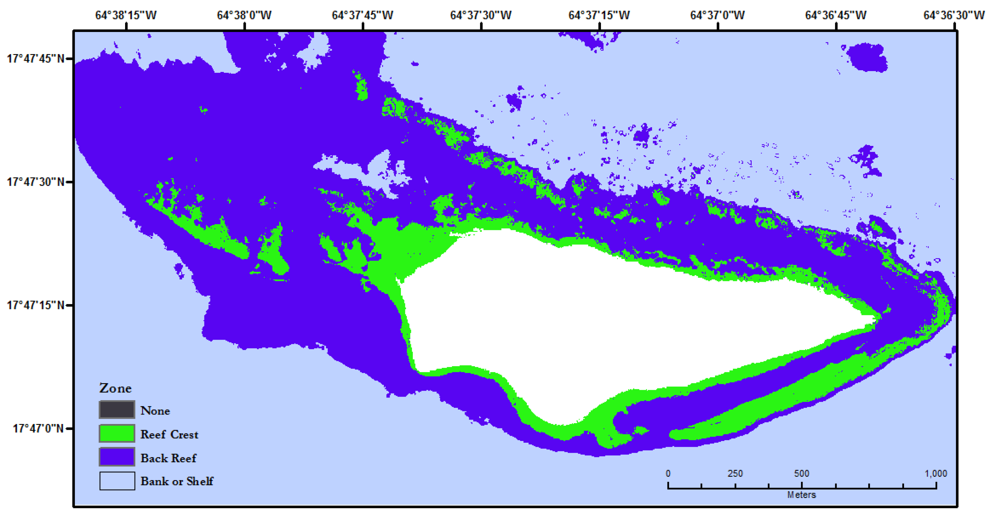
Figure 9.
Output from the summary() function on the results from the principal component analysis to explain the proportion of variance explained by each selected covariate.
Figure 9.
Output from the summary() function on the results from the principal component analysis to explain the proportion of variance explained by each selected covariate.
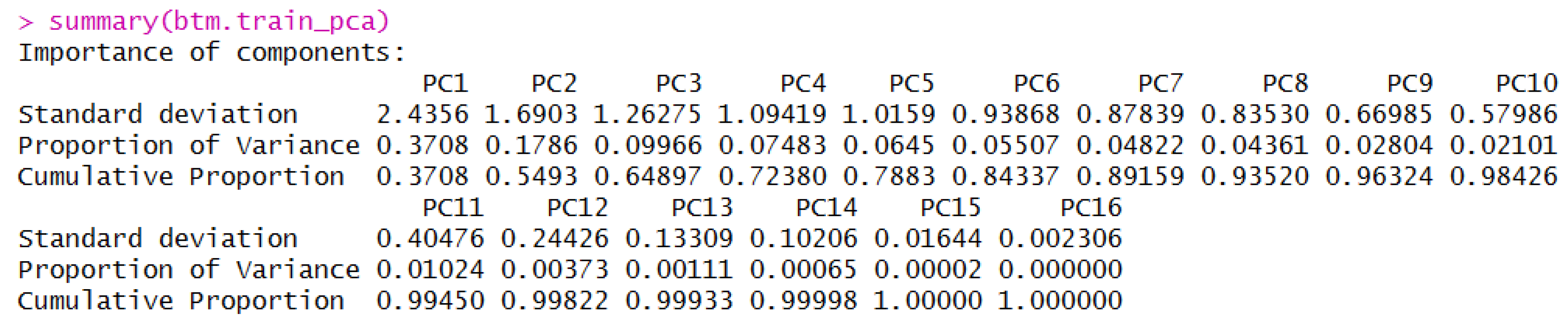
Figure 10.
Output from the plot() function on the results from the principal component analysis which show the components that explain 95 percent of the variance.
Figure 10.
Output from the plot() function on the results from the principal component analysis which show the components that explain 95 percent of the variance.

Figure 11.
Left: planar slope, , in degrees. Center: geodesic slope, , in degrees. Right: Slope differences, (), with the displayed range of (1 to -1). Most areas show very small changes in the values, but locations with high rugosity, and steep slopes show localized larger differences. Same inset locations described in Figure 2.

Table 1.
Terrain attributes computed by Benthic Terrain Modeler.
| Name | Algorithm | Notes | References |
|---|---|---|---|
| Slope | Computed over a neighborhood | [18] | |
| Statistical Aspect | Generates Easterness and Northerness | [19,20] | |
| Mean Depth | n is the size of a square neighborhood of cells | ||
| Standard Deviation | is the mean elevation of cells within the analysis neighborhood | ||
| Variance | is the standard deviation of a neighborhood of cells | ||
| Interquartile Range | is the cumulative distribution function of all cells in the analysis neighborhood | [21] | |
| Kurtosis | is the fourth central moment and is the standard deviation of all cells in the analysis neighborhood | [21] | |
| BPI | is the mean elevation value of all cells within an annulus-shaped neighborhood | [12] | |
| VRM | see Section 2.1.3 | [22] | |
| SAPA | see Section 2.1.3 | [23] | |
| SAPA (Slope-corrected) | see Section 2.1.3 | Decoupled from slope as per ACR | [24] |
| ACR | see Section 2.1.3 | [24] |
Table 2.
Benthic Terrain Modeler Interfaces.
| Interface | Role |
|---|---|
| Graphical menu | Direct interaction (see Figure 6) |
| Python toolbox | Direct and scripted interaction |
| Command-line | Reproducible, scalable, programmatic |
| Jupyter Notebooks | Teaching and exploration |
Table 3.
Classification table used for creation of Figure 8. Missing values indicate that the bound is not applicable to the benthic zone.
Table 3.
Classification table used for creation of Figure 8. Missing values indicate that the bound is not applicable to the benthic zone.
| Class | Zone | Broad BPI (Lower) | Broad BPI (Upper) | Fine BPI (Lower) | Fine BPI (Upper) | Slope (Lower) | Slope (Upper) | Depth (Lower) | Depth (Upper) |
|---|---|---|---|---|---|---|---|---|---|
| 1 | Reef Crest | −87 | 541 | −907 | 2229 | 11 | −2 | ||
| 2 | Back Reef | −87 | 541 | −459 | 885 | 52 | −6 | ||
| 3 | Bank or Shelf | −402 | 699 | −1355 | 4469 | 74 | −18 | ||
| 4 | Reef Flat | −9 | 541 | −459 | 1333 | 67 | −8 | ||
| 5 | Channel | −323 | 384 | −907 | 1333 | 53 | −12 | −1 | |
| 6 | Fore Reef | −323 | 541 | −1355 | 2229 | 61 | −14 | ||
| 7 | Lagoon | −166 | 463 | −459 | 1333 | 49 | −7 | ||
| 8 | Salt Pond | −9 | −9 | −11 | −11 | 53 | −7 | ||
| 9 | Shoreline Intertidal | −9 | 384 | −11 | 436 | 19 | −2 |
Table 4.
Parameters used for benthic classification in Run All Model Steps tool.
| Parameter | Value |
|---|---|
| Bathymetry Raster: | LiDAR bathymetry (clipped) |
| Broad-scale BPI Inner Radius: | 25 |
| Broad-scale BPI Outer Radius: | 250 |
| Fine-scale BPI Inner Radius: | 5 |
| Fine-scale BPI Outer Radius: | 25 |
| Classification Dictionary: | See Table 3 |
© 2018 by the authors. Licensee MDPI, Basel, Switzerland. This article is an open access article distributed under the terms and conditions of the Creative Commons Attribution (CC BY) license (http://creativecommons.org/licenses/by/4.0/).
Share and Cite
MDPI and ACS Style
Walbridge, S.; Slocum, N.; Pobuda, M.; Wright, D.J. Unified Geomorphological Analysis Workflows with Benthic Terrain Modeler. Geosciences 2018, 8, 94. https://doi.org/10.3390/geosciences8030094
AMA Style
Walbridge S, Slocum N, Pobuda M, Wright DJ. Unified Geomorphological Analysis Workflows with Benthic Terrain Modeler. Geosciences. 2018; 8(3):94. https://doi.org/10.3390/geosciences8030094
Chicago/Turabian StyleWalbridge, Shaun, Noah Slocum, Marjean Pobuda, and Dawn J. Wright. 2018. "Unified Geomorphological Analysis Workflows with Benthic Terrain Modeler" Geosciences 8, no. 3: 94. https://doi.org/10.3390/geosciences8030094
Note that from the first issue of 2016, this journal uses article numbers instead of page numbers. See further details here.