Bathymetry and Canyons of the Eastern Bering Sea Slope


1
National Marine Fisheries Service, NOAA, Alaska Fisheries Science Center, 7600 Sand Point Way NE, Bldg. 4, Seattle, WA 98115-6349, USA
2
Lynker Technologies, Under contract to Alaska Fisheries Science Center, 7600 Sand Point Way NE, Bldg. 4, Seattle, WA 98115-6349, USA
*
Author to whom correspondence should be addressed.
Geosciences 2018, 8(5), 184; https://doi.org/10.3390/geosciences8050184
Submission received: 28 February 2018
/
Revised: 9 May 2018
/
Accepted: 15 May 2018
/
Published: 21 May 2018
(This article belongs to the Special Issue Marine Geomorphometry)
Abstract
:We created a new, 100 m horizontal resolution bathymetry raster and used it to define 29 canyons of the eastern Bering Sea (EBS) slope area off of Alaska, USA. To create this bathymetry surface we proofed, edited, and digitized 18 million soundings from over 200 individual sources. Despite the vast size (~1250 km long by ~3000 m high) and ecological significance of the EBS slope, there have been few hydrographic-quality charting cruises conducted in this area, so we relied mostly on uncalibrated underway files from cruises of convenience. The lack of hydrographic quality surveys, anecdotal reports of features such as pinnacles, and reliance on satellite altimetry data has created confusion in previous bathymetric compilations about the details along the slope, such as the shape and location of canyons along the edge of the slope, and hills and valleys on the adjacent shelf area. A better model of the EBS slope will be useful for geologists, oceanographers, and biologists studying the seafloor geomorphology and the unusually high productivity along this poorly understood seafloor feature.

1. Introduction
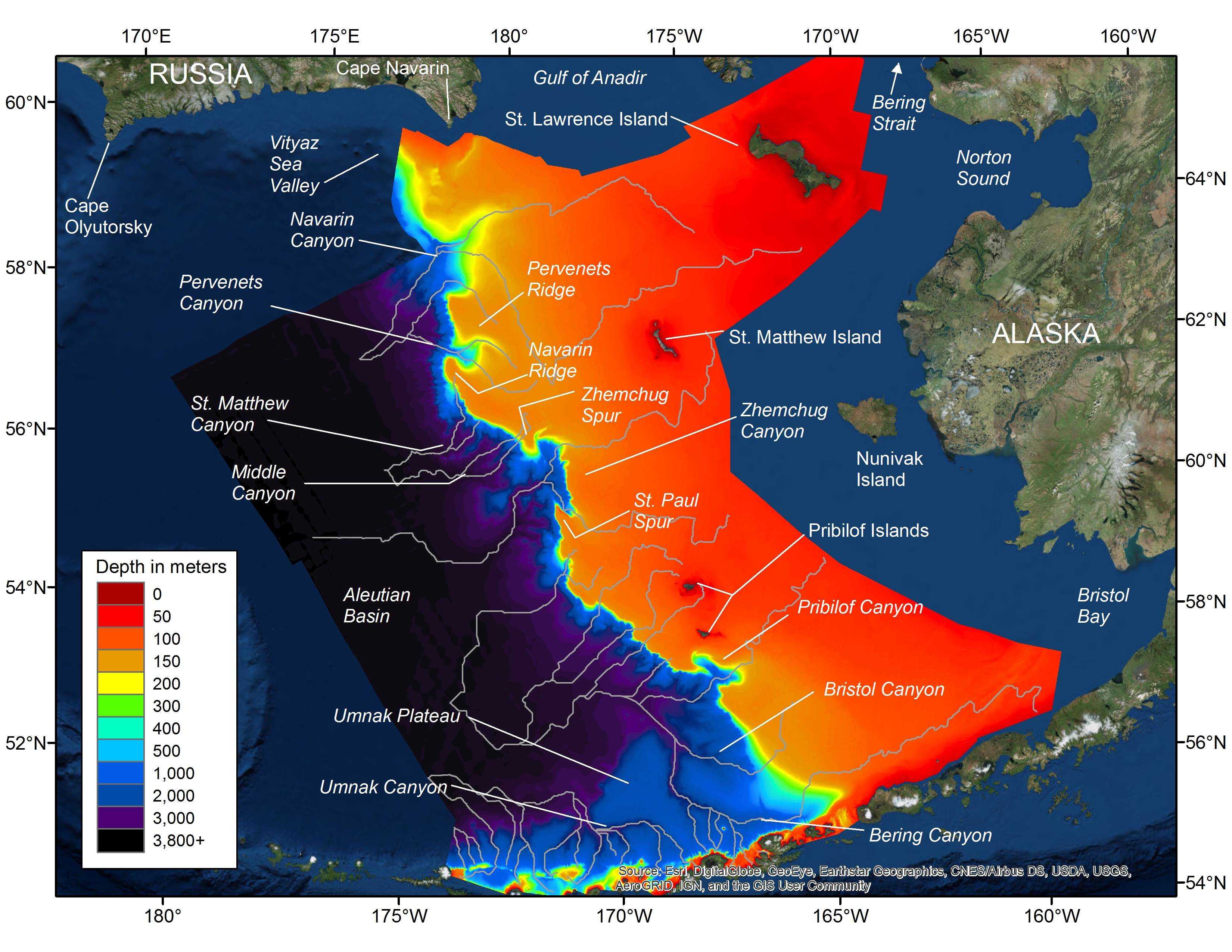
The eastern Bering Sea (EBS) slope is an abrupt, sinuous seafloor feature, ranging approximately 1250 km in length from Bering Canyon in US waters to the Vityaz Sea Valley in Russian waters (Figure 1). Depths to the east of the slope on the Bering Sea shelf are shallow (~130 m), depths to the west of the slope in the Aleutian Basin are deep (>3000 m), and numerous canyons, some of which are the largest in the world [1], scallop the edge of the shelf. This vast vertical and horizontal expanse of seafloor has been only partially explored and charted. The only land along the EBS slope is the Pribilof Islands, so navigating with visual fixes to triangulation shore stations, the traditional and primary method used by the National Ocean Service (NOS, Silver Spring, MD, USA) for producing smooth sheets [2] was not well-suited to this area. The absence of high quality smooth sheets, which are the detailed records of the original charting surveys, is a major detriment to understanding the bathymetry in this area. While the Aleutian Islands (AI) portion of this area was well-charted with smooth sheets mostly in the late 1930’s [3], the waters surrounding islands in the Bering Sea such as St. Matthew Island (1951), the Pribilof Islands (1951–53), and St. Lawrence Island (1951–54, 1968–70) were charted much later, incompletely, and often at small scales. The Aleutian Basin (1952) and portions of the EBS slope (1951–53) were only charted at a coarse scale of 1:500,000.
1.1. Early Charting of the Eastern Bering Sea Slope and Canyons
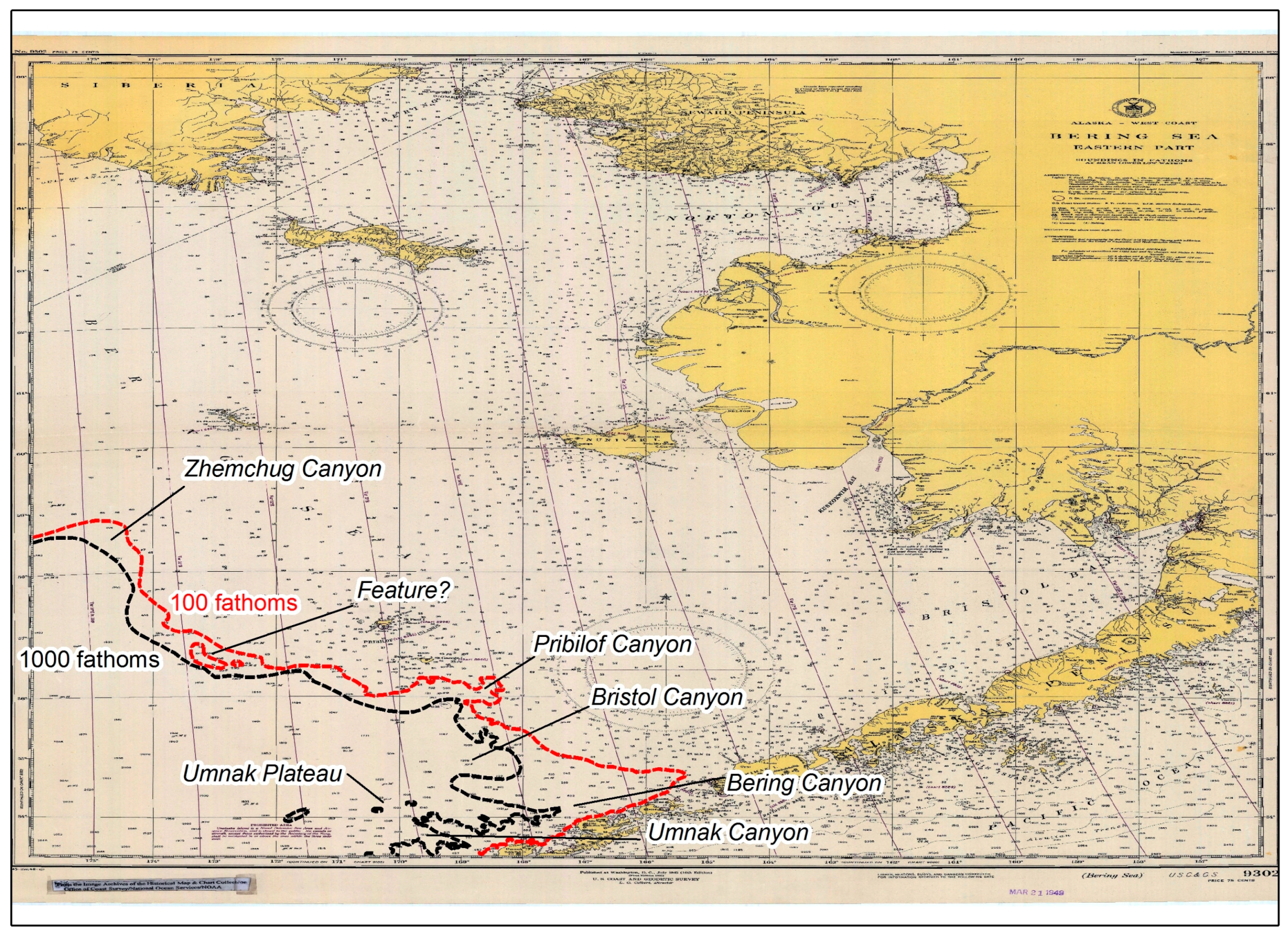
Prior to 1950, the EBS slope and a few canyons were only partially depicted with 100 and 1000 fathom contours on the most detailed US chart (9302) of this area (Figure 2). While Bering Canyon was clearly placed at the intersection between the slope and the Aleutian Islands, and portions of adjoining Umnak Canyon were depicted, Pribilof Canyon was only vaguely outlined, and none of the northern canyons (Zhemchug, Middle, St. Matthew, Pervenets, and Navarin) were known. Many of the soundings depicted on Chart 9302 are from Albatross cruises conducted in the late 1800s.
In the early 1950s, the NOS coarsely charted the US portion of the slope from the Aleutian Islands up to 59°30′ N. Pervenets and Zhemchug Canyons were clearly depicted on smooth sheet H08103 (1953, Scale 1:500,000) but only assigned the generic name of “Marine Canyon” in the descriptive report (https://data.ngdc.noaa.gov/platforms/ocean/nos/coast/H08001-H10000/H08103/DR/H08103.pdf). Zhemchug Spur (945 fathoms or 1728 m) and two ridges on St. Paul Spur (northern ridge as shallow as 47 fathoms or 86 m, southern ridge as shallow as 51 fathoms or 93 m) were also charted by H08103 but only identified as notable shallow soundings. Smooth sheet H07949 (1951–53, Scale 1:500,000) covered the southern half of the US portion of the slope, but a digital version of the smooth sheet is not available for analysis, and no seafloor features were named in the descriptive report (https://data.ngdc.noaa.gov/platforms/ocean/nos/coast/H06001-H08000/H07949/DR/H07949.pdf).
The Russian fishery research vessel Zhemchug explored and named four large canyons in the mid- to late-1950s: Navarin Canyon (1955), Pervenets Canyon (1958, along with the R/V Pervenets), Pribilof Canyon (1958), and Zhemchug Spur and Canyon (1959) (https://www.ngdc.noaa.gov/gazetteer/). The Russians were probably unaware of the earlier US mapping effort, as smooth sheets H07949 and H08103 were routinely classified as confidential by the US government. Following the new knowledge gained in the 1950s, the 1967 version of NOS chart 8802 (Scale 1:1,023,188) shows a much more definitive Pribilof Canyon and the 1968 version of chart 9302 (Scale 1:1,534,076) shows Zhemchug Canyon, a few soundings from Zhemchug Spur, and a single, shallow sounding representing the two St. Paul Spur ridges.
St. Matthew and Middle Canyons [4] were discovered in the northern slope area by the USGS (US Geological Survey) in the early 1980s [5,6,7]. Some northern canyon metrics, such as areas and volumes, were described [7]. In 1986, an early version of sidescan sonar (GLORIA: Geological LOng-Range Inclined Asdic) was used to map the backscatter of the Aleutian Basin and eastern Bering Sea shelf edge, including the major canyons (see https://pubs.usgs.gov/of/2010/1332/), and the towing vessel Farnella provided a path of singlebeam depths, which was a significant mapping contribution to the Aleutian Basin.
Multibeam surveys are rare in the EBS slope. In 2003, a 210 km section of the Beringian Margin near Pervenets Canyon was mapped from depths of ~1000 to 3700 m (http://ccom.unh.edu/theme/law-sea/beringian-margin-bering-sea). The NOS has been multibeam mapping in the Unimak Pass area since the mid-2000s (https://maps.ngdc.noaa.gov/viewers/bathymetry/). Pribilof Canyon was mapped with multibeam in 2009, making it the only EBS slope canyon with accurate bathymetry (https://data.ngdc.noaa.gov/platforms/ocean/nos/coast/H12001-H14000/H12115/DR/H12115.pdf).
1.2. Chart 16006 and the Zhemchug Canyon Pinnacles
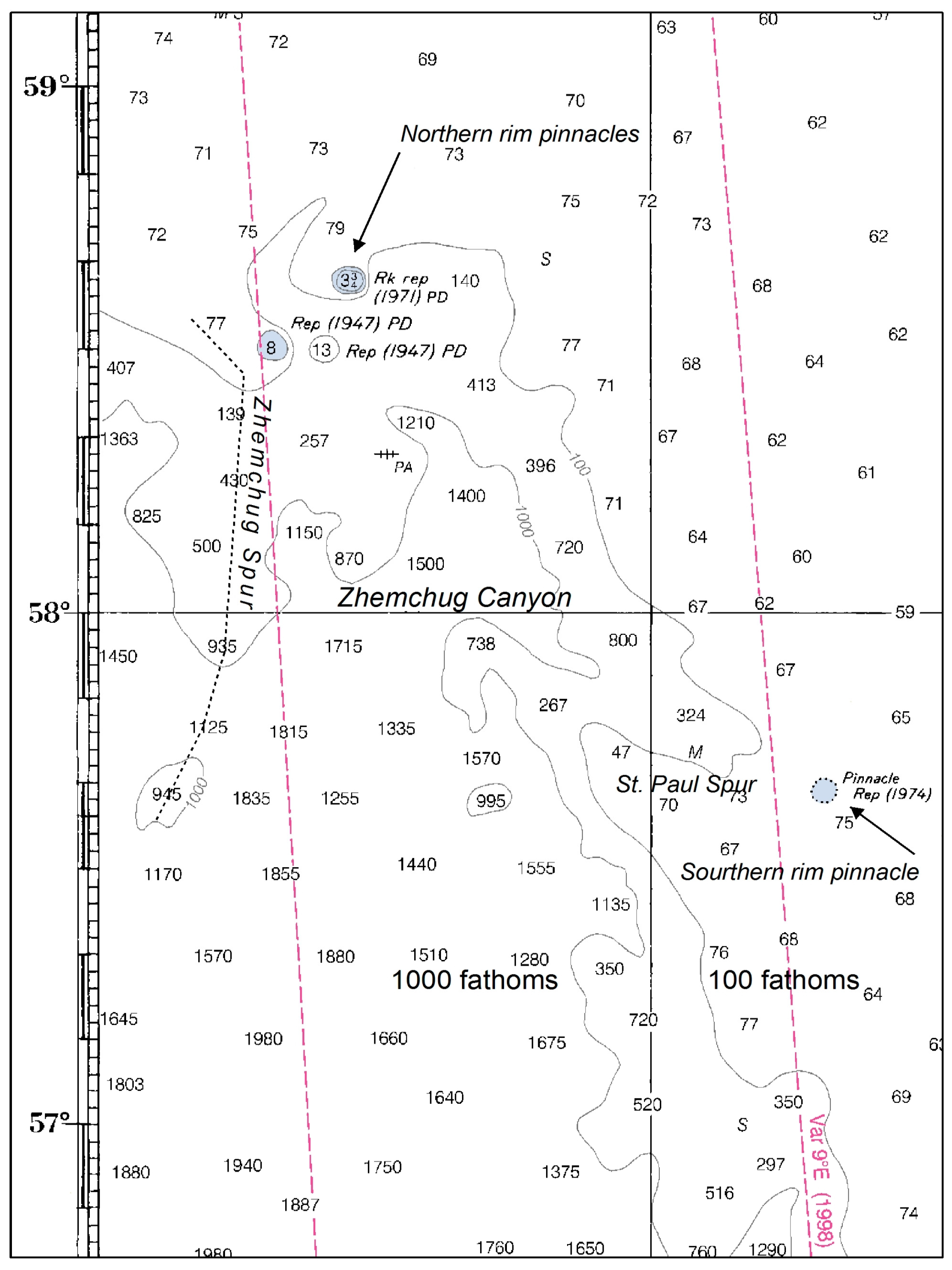
There are four pinnacles reported to be in the Zhemchug Canyon area (Figure 3). Discoveries of previously unknown and dangerous pinnacles, such as the 650 ft (198.1 m) tall “Washington Monument” pinnacle in South East Alaska, rising to a depth of just 2.75 fathoms (5.0 m), have been a very real reminder of the danger for navigation in Alaska’s uncharted waters for over a century [8]. The Zhemchug Canyon pinnacles are legendary and members of the research, environmental, and commercial fishing communities are all familiar with their vague and inconvenient location in relatively deep water along the edge of the Bering Sea self.
The Zhemchug Canyon pinnacles originated with the US submarine Bergall, which surfaced during its first training patrol in the northern portion of Zhemchug Canyon and reported a day time sounding of 8 fathoms (14.6 m) on 19 April, 1947 and a nearby sounding of 13 fathoms (23.8 m) on the following day (https://data.ngdc.noaa.gov/platforms/ocean/nos/coast/H06001-H08000/H07951/DR/H07951.pdf). In response to this US Navy report of pinnacles, survey H07951 (smooth sheet not available) was conducted in 1951; the USS Bergall pinnacles were disproved, and no pinnacles were reported on the most detailed NOS chart of this area (NOS Chart 9302, Scale 1:1,600,000) through the 1971 edition (22nd edition). The third pinnacle (3.75 fathoms or 6.9 m) was reported, potentially by Russia, in 1971 through the Notice to Mariners (http://msi.nga.mil/NGAPortal/MSI.portal?_nfpb=true&_pageLabel=msi_portal_page_61), and the next edition of NOS Chart 9302 (1973) had the first depiction on a US navigational chart of this new pinnacle, as well as the two previously disproven USS Bergall pinnacles. Chart 9302 was replaced by Chart 16006 in 1975, and that edition adds the fourth and final pinnacle, this one—of unknown depth, near the southern edge of Zhemchug Canyon—was reported to the Notice to Mariners by the US Coast Guard Cutter Jarvis on 10 May, 1974.
1.3. Bathymetry Compilations, Oceanographic and Biological Research
Global and regional bathymetry compilations of various bathymetric sources have advanced our knowledge of the Alaska seafloor. Global bathymetry surfaces of 2 arc-minute resolution (~3704 m) [9], 1 arc-minute resolution (~1852 m) (ETOPO1: [10]), and 30 arc-second resolution (~926 m) (General Bathymetric Chart of the Oceans, GEBCO: [11]) were published using a mixture of soundings and calibrated remote sensing data. Regional bathymetry compilations include those of the AKRO (National Marine Fisheries Service, Alaska Regional Office (Anchorage, AK, USA): https://alaskafisheries.noaa.gov/, variable resolution, 2005; updated to 40 m resolution in 2017, https://inport.nmfs.noaa.gov/inport/item/27377), the International Bathymetric Chart of the Arctic Ocean (IBCAO 3.0, 500 m resolution, [12]), and the Alaska Regional Digital Elevation Model, which is a compilation that includes US and Russian chart soundings (ARDEM, ~1 km resolution, [13]).
A global analysis of canyons was conducted using the ETOPO1 data set [14], producing 26 thalwegs within our study area. Additional seafloor features in the EBS slope area were defined from Shuttle Radar Topography Mapping (SRTM30_PLUS) in another global analysis [15]. Locations and names of seafloor features—mostly canyons—were available from GEBCO (https://www.gebco.net/data_and_products/undersea_feature_names/) and the National Geospatial Intelligence Agency (NGA, Springfield, VA, USA: https://www.ngdc.noaa.gov/gazetteer/).
Marine researchers have benefitted greatly from these bathymetry compilations and subsequent geomorphological analyses, but still there has been an unmet need for more detailed and more accurate depth data for fisheries habitat studies at the Alaska Fisheries Science Center (AFSC, Seattle, WA, USA). To meet this need, we have been publishing 100 m resolution bathymetry compilations in recent years: AI [3], Cook Inlet (50 m resolution: [16]), Norton Sound [17], and central Gulf of Alaska (GOA, AK, USA) [18]. These bathymetry compilations have been utilized for a variety of fishery research purposes including fish vertical migration [19]; coral and sponge distribution modeling in the AI [20] and GOA [21]; quantifying inshore study sites in the central GOA [22], eastern GOA [23], and bathymetry groundtruthing [24]; bathymetric steering of seafloor current flow [25]; inshore habitat loss [26]; Essential Fish Habitat modeling in the EBS [27], GOA [28,29], and AI [30]; juvenile groundfish habitat suitability models [31]; and capelin (Mallotus villosus) distribution modeling [32].
The EBS slope area is important for several commercial fisheries, and the impact of these fisheries has been the focus of significant research. The majority of the commercial fishery for walleye pollock (Gadus chalcogrammus)—the largest fishery in the world [33]—takes place on the slope and adjoining shelf. The biological importance of the canyons versus the inter-canyon areas was examined (https://www.npfmc.org/bering-sea-canyons/; [34,35,36]), and there has been interest in documenting the ecosystem function of pinnacles in the Zhemchug canyon area [pers. comm. John Hocevar 2017]. Skate egg case nurseries for three species of Bathyraja are found in the canyons [37], and biannual stock assessment bottom trawl surveys for several commercially important species are conducted at depths of 200 to 1200 m along the slope [38].
The EBS slope is an area of particular oceanographic and biological importance beyond just fish, corals, and sponges. For example, the slope plays an important role in limiting the extent of winter ice formation on the EBS shelf [39] (see Figure 3). Researchers coined the term “Bering Sea Green Belt” to describe the productivity of the EBS slope (see Figure 2) [40], summarized the flow of ocean currents; and plotted the peak abundances of phytoplankton, zooplankton, squids, fishes, sea birds, and mammals along this shelf edge. Wong et al. [41] demonstrated that it was an important habitat for marine birds such as red-legged (Rissa brevirostris) and black-legged kittiwakes (R. tridactyla); northern fulmars (Fulmarus glacialis); sooty, great, and short-tailed shearwaters (Puffinus griseus, P. gravis, P. tenuirostris, respectively); fork-tailed, Leach’s, and Wilson’s storm-petrels (Oceanodroma furcata, O. leucorhoa, and Oceanites oceanicus, respectively); surface and diving piscivores; and surface and diving planktivores. The North Pacific Pelagic Seabird Database also shows that this area is important for the endangered short-tailed albatross (Phoebastria albatrus) (https://alaska.usgs.gov/science/biology/nppsd/index.php), one of the rarest marine birds in the world. A better depiction of the slope and canyons should improve our understanding of how this undersea feature affects so many physical and biological aspects of the EBS.
2. Materials and Methods
2.1. Bathymetry Data Sources and Typical Errors
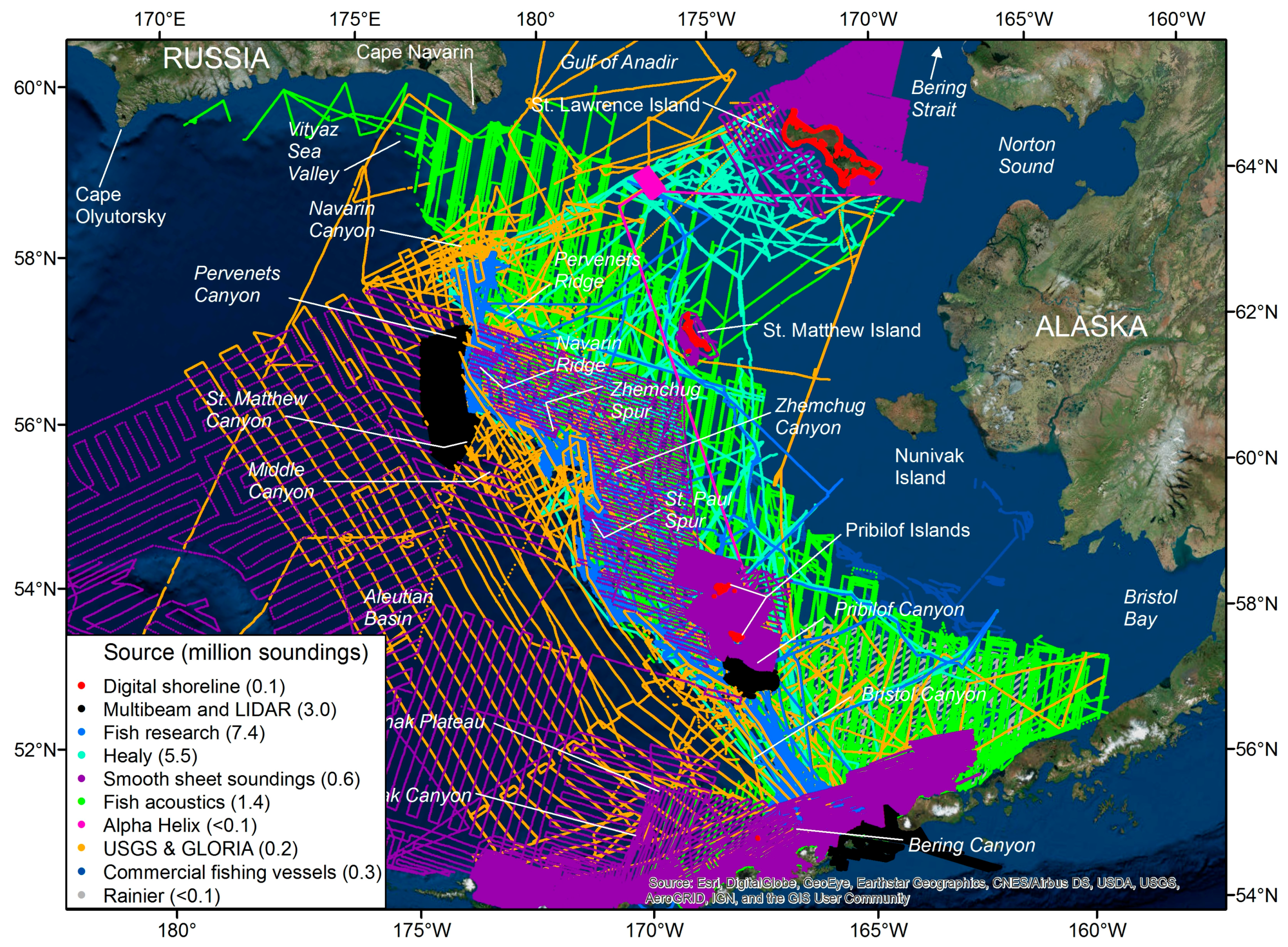
We utilized 18 million soundings from over 200 individual sources that can be grouped into ten general categories, each of which came with its own advantages and disadvantages (Figure 4). Initially, we edited each file by searching for outliers (e.g., depths of zero) or incorrect positions. When possible, we corrected or deleted errors by comparing depth values to original sources (e.g., smooth sheets and echosounder files). We also rejected soundings that overlapped with a data set we judged to be superior. Reducing overlaps of data sets from the 10 different sources helped to minimize disagreements and avoid conflicts such as differing vertical datums, as nearshore surveys were generally corrected to a vertical tidal datum, while offshore surveys generally were not corrected. NOS smooth sheets and multibeam surveys covered only a small amount of the study area and, therefore, we had to rely heavily on other bathymetric sources. Unpublished underway files, either collected from navigational software or extracted from the raw echosounder files, covered the vast majority of this project area.
2.1.1. Smooth Sheets and Multibeam
Most smooth sheet and all multibeam data were collected at a vertical datum of Mean Lower Low Water (MLLW). In general, offshore smooth sheets, such as those soundings depicted northwest of the Pribilof Islands and those covering the Aleutian Basin, are not corrected to any vertical datum and thus are considered to approximate Mean Sea Level (MSL). For example, the Aleutian Basin soundings were collected at depth intervals of 5 to 10 fathoms (9.1 to 18.3 m) in recognition of the fact that inaccuracies in speed of sound estimates, poor navigation (due to vast distance from shore stations), heave, and errors in distinguishing the exact start of the seafloor reflection far exceeded tidal differences. Smooth sheet soundings (digital files available at https://www.ngdc.noaa.gov/) [42] for this compilation had errors that were familiar to us [43] from previous compilations, including improper horizontal datum shifting, random digitization errors, and undigitized soundings—for example, smooth sheets H08103 and H08001B needed to be digitized entirely.
We downloaded the National Geodetic Survey shorelines (NOAA Shoreline Explorer web site: http://www.ngs.noaa.gov/NSDE/) for the Pribilof Islands and St. Lawrence Island, and annotated them with MHW (mean high water) from corresponding NOS smooth sheets. The MLLW and MHW vertical datums are compatible with each other and utilized on every navigational chart of Alaska. This useful resource provides shoreline very similar to that of the smooth sheets, but derived from a different survey product, sometimes contradicting findings from the smooth sheet inshore work. We also digitized the shoreline from the smooth sheets for Bogoslof Island and St. Matthew Island, again annotating them with MHW from the corresponding smooth sheets.
All multibeam data sets were subsampled to a resolution of 100 m. The UNCLOS (United Nations Convention of the Law of the Sea) multibeam from the Bering Margin (http://ccom.unh.edu/theme/law-sea/law-of-the-sea-data/bering-sea) reported positions in decimal latitudes and longitudes, rather than in projected meters, resulting in off-center raster cells.
The 1970 cruise of the Rainier, a NOS hydrographic vessel, provided an underway file that was similar in resolution to that of the smaller scale NOS smooth sheets, although it was a USGS research cruise (https://walrus.wr.usgs.gov/infobank/r/r170bs/html/r-1-70-bs.meta.html). This cruise was collected without tidal correction and thus is at a vertical datum of MSL.
2.1.2. Underway Files
Underway files, collected without tidal correction and without heave correction, are similar to the 1970 Rainier cruise. Thus, the underway files approximate a vertical datum of MSL. These underway files typically had random depth errors but were most significantly plagued with the echosounder losing track of the seafloor and either repeating a depth for long distances or creating false depths by incorrectly recording reflections from a mid-water scattering layer. Both of these “lost seafloor” sources of error were difficult to detect, as repeated depths on the EBS shelf were common because the shelf is extremely flat, while depths along the slope were often unknown in areas of rapid depth change.
The Alpha Helix mooring recovery cruise of 2004 (http://www.rvdata.us/catalog/HX291) provided an unusually thorough, gridded search pattern of underway soundings between Navarin Canyon and St. Lawrence Island due to the unfortunate loss of a mooring [Pers. comm. Cal Mordy, 2015].
AFSC EBS slope bottom trawl biennial cruises (e.g., [38]) provided underway files from Seaplot software, Globe software, or bottom picks from EchoView analysis of raw echosounder files. Random and “lost seafloor” errors were also common in this source, but each cruise was different and had to be proofed and edited carefully. For example, one cruise collected soundings in fathoms for over one hundred km before switching to meters—the standard for all other cruises. Additional AFSC fish research cruises on the Zhemchug ridges (SCS Miller Freeman 2007 and Globe 2008 F/V Vesteraalen) provided detailed parallel transects [44]. These appear to be the only AFSC cruises conducted for seafloor mapping purposes on the EBS slope.
AFSC walleye pollock acoustic cruises covering the Bogoslof Island area (e.g., [45]) or the outer EBS shelf and slope area (e.g., [46]) occur on an almost annual basis. Older Miller Freeman data were in the format of depth averaged across distance along transects; no raw acoustic files or individual soundings are available (1991–1996). Underway files of raw soundings, typically collected at 30 second intervals, were recorded in more recent years with Scientific Collection System software (https://www.unols.org/sites/default/files/200110rvtap16.pdf) on the Miller Freeman (1997–2006) and the Oscar Dyson (2007–2016). These more recent pollock surveys accounted for hull depth but had the same types of errors as in other underway sources (random and “lost seafloor” errors), but much less frequently. We attempted to incorporate data from the F/T Continuity cruise of 1991 and the Miller Freeman cruise of 1992, but depths from these cruises disagreed with all other cruises—we also had to delete data from legs 1 and 2 of the 1994 Miller Freeman cruise but were able to utilize data from leg 3.
BEST (Bering Sea Ecosystem Study: https://www.eol.ucar.edu/projects/best/) cruises on the US Coast Guard Cutter Healy (2006–2009) seemed to have higher incidences of random errors, and we screened sections of transects by examining for continuous distribution of depths, deleting soundings outside of a central range of values. Northern portions of transects, which appear to have been conducted in the sea ice, had too many random depth errors to use in this project.
Commercial fishery vessel depth data were all from Globe files, and these typically only had random errors. A benefit of this source was that vessels tended to conduct new tracks adjacent to previous tracks, which provided depth data over new areas, rather than consistently on top of old tracks, as in research cruises.
USGS explorations (https://cmgds.marine.usgs.gov/) utilized various vessels (Discoverer 1980–81; Sam Phillips Lee 1975–1983; Sea Sounder 1976–77; and Maurice Ewing 1994). These cruises seemed to suffer from navigational errors, similar to the smooth sheets, but were able to produce reliable depths in deep water. GLORIA cruises conducted on the Farnella (1986) produced depths in the Aleutian Basin (>3000 m), which were generally deeper than overlapping smooth sheet depths. With two-way travel time sometimes exceeding five seconds for a sounding, we suspected that the difference in depth between the two data sets is due to differences in speed-of-sound utilized for estimating depth. However, the GLORIA data utilized speed-of-sound estimates [pers. comm. Jim Gardner, 2017] derived from Carter [47] or field observations, and these were generally slower than used by the smooth sheets (1500 m/s). Thus, attempts to correct one data set to the other by correcting for speed-of-sound differences resulted in greater differences; therefore, we did not perform this correction.
2.2. Bathymetry Raster Creation
Smooth sheet bathymetry formed the foundation of this compilation, as in all of our previous compilations, but smooth sheets covered a smaller area than in our previous compilations. We reused smooth sheet bathymetry from our AI compilation [3] for the southern portion of this compilation to provide a more complete spatial extent of the EBS slope. Most of the effort on this project was devoted to proofing and editing the underway files, which, along with covering the majority of the area also seemed to have the bulk of the errors. For the first time in our bathymetry compilations, we encountered the problem that the edited underway files from vessels with GPS navigation, but with completely uncalibrated echosounders, often exceeded the quality of the smooth sheets, which were small scale (1:500,000). Therefore we eventually had to delete large areas of smooth sheet soundings to construct this bathymetric surface. Multibeam data only covered about two percent of our study area. All data sets (smooth sheets, multibeam, and underway files) were combined to create TINs (Triangulated Irregular Networks). In an iterative process, TINs were plotted with color ramps for slope (see Figure 30 in reference [43]) and depth to reveal sounding outliers to target for editing. After numerous rounds of editing, the TIN was converted to a raster of 100 m horizontal resolution by using local area weighting (termed natural neighbors in ArcMap), a method and resolution that has worked well in our previous compilations [2], refs. [16,17,18] for depicting seafloor features as detailed as earthquake faults with low resolution data [18]. Our final raster surface is a mix of onshore MLLW and offshore MSL data sets, as NOAA’s vertical datum tidal correction software is not available for Alaskan waters (https://vdatum.noaa.gov/about.html).
2.3. Thalweg Creation
We determined the location, size, and number of canyons within our compilation by utilizing the Hydrology toolbox in ArcMap (v.10.2.2, ESRI: Environmental Systems Research Institute, Redlands, CA, USA). In this method, raster cells are examined to determine how water would flow downhill based on depth, slope, and aspect; sinks are filled; and then the few cells that receive the most calculated runoff (we set our lower limit as >1000 cells) are labeled as rivers. Runoff may only travel in the eight cardinal or inter-cardinal compass directions, so straight river sections are common, and parallel river sections are allowed. In our submerged environment we treat these “rivers” as thalwegs to define the center-lines of canyons. We conducted this analysis with both positive and negative depth surfaces to create thalwegs and ridgelines, both of which helped identify cruises that were slightly (~1 m) shallower or deeper than other cruises. Underway cruises with the largest depth errors were compared to multibeam depths by using the Ordinary Least Squares function in ArcMap:
in which y are the underway soundings and x are the multibeam depths. To make the depth correction, we subtracted the y-intercept (b) from the underway depths and divided by the slope (m):
y = m × x + b,
(y − b)/m = x,
As thalweg creation was still highly sensitive to cruises with depth errors that were too small to correct with multibeam comparisons, we smoothed the bathymetry raster with a low pass filter using a rectangular neighborhood of 20 cells. Thalwegs were then created from the smoothed surface, but canyon metrics were derived by comparing the thalweg paths to the unsmoothed 100 m resolution bathymetry and slope surfaces. A shape file of the thalwegs is provided as Supplementary Material with this manuscript (Thalwegs.zip).
2.4. Zhemchug Canyon Pinnacles
We digitized the warning circles drawn on NOS Chart 16006 around each of these pinnacles and extracted the corresponding soundings from our compilation. We examined these soundings for any indication of the pinnacles.
3. Results
3.1. Eastern Bering Sea Slope Bathymetry
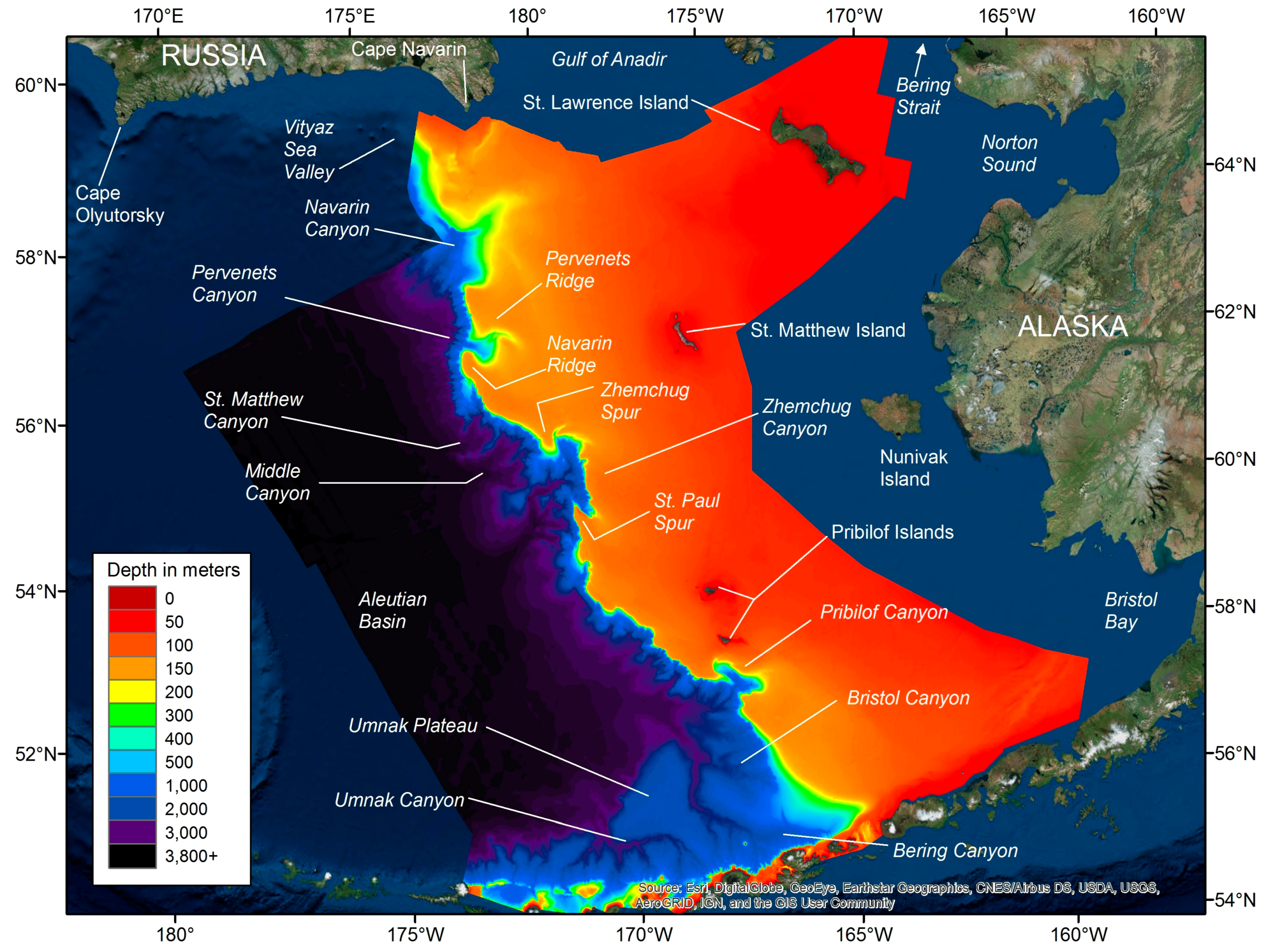
Our bathymetry compilation (Figure 5) covered almost one million km2, spanning 1400 km from west to east and 1300 km from north to south, joining our Norton Sound compilation [17] in the north and overlapping with our AI compilation in the south [3]. Imagery of the bathymetry is provided as Supplementary Material with this manuscript (EBS Slope Bathymetry.zip). We compared our bathymetry surface to previously published cartographic information of the area: seafloor gazetteers from GEBCO and NGA, NOS navigation Chart 16006 (as the source for the Zhemchug Canyon pinnacles), published geomorphic features, and other bathymetry compilations. We attempted to reconcile differences between our bathymetry compilation results and the seafloor interpretations of others in order to minimize cartographic confusion. NOS Chart 16006 is still the most detailed US navigational chart of the area, and still only uses the 100 and 1000 fathom depth contours to describe the EBS slope. Previously published canyon shape parameters and thalwegs [14], and geomorphology polygons [15], were also used for comparisons. Global and regional bathymetry compilations utilize a wide variety of input data sets and publish at several different resolutions.
3.2. Eastern Bering Sea Slope Canyon Thalwegs
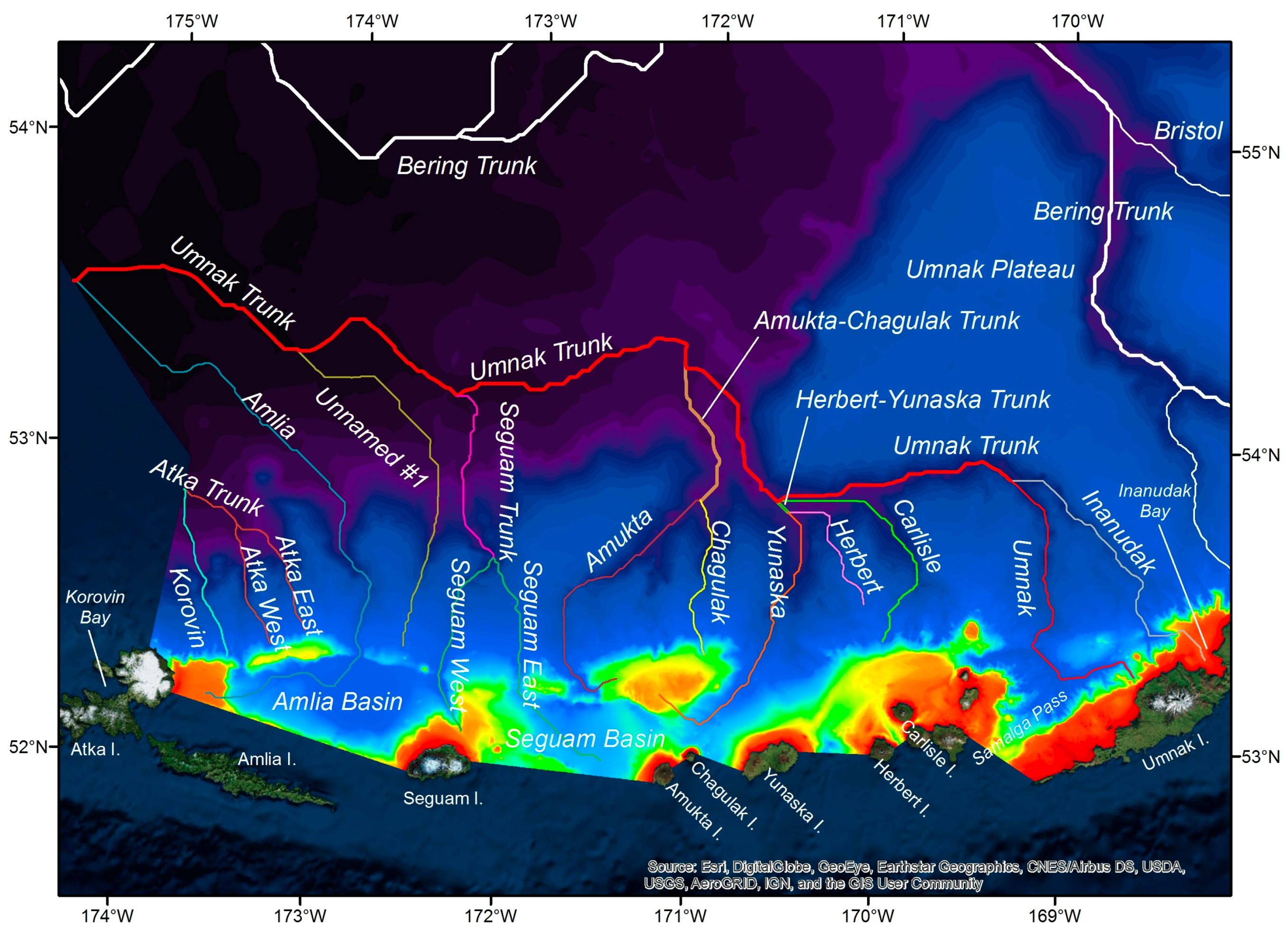
Umnak Canyon occupied the southern portion of our compilation, running roughly parallel to the Aleutian Islands, with several smaller canyons running perpendicular to the main Umnak Trunk. The southeastern area was dominated by Bering Canyon and several other connected or nearby canyons, including Bristol and Pribilof Canyons. Navarin and Zhemchug Canyons occupied most of the northern slope. The thalwegs north of Navarin Canyon and around St. Lawrence Island did not connect with the EBS slope canyons, indicating that the bathymetry compilation extended sufficiently far north in extent, but the Bering, Pribilof, Zhemchug, and Navarin Canyon thalwegs reached near the eastern edge of our bathymetry compilation, suggesting that this portion of the compilation could be expanded. The interior section of Bristol Bay and adjoining shallow areas were not included in this project but may be the subject of a future compilation.
3.2.1. Umnak Canyon Thalwegs
The GEBCO gazetteer only names 5 canyons (plus a canyon basin) in the Umnak area, while the NGA gazetteer repeats these same features and adds 7 more canyons, all extending northward from the Aleutian Islands into deeper water, to a large and deep canyon (Figure 6, Table 1). Starting on the western side, our thalwegs agree with NGA’s placement of Korovin Canyon. To the east of Korovin is Atka Canyon, and the NGA label is on a western thalweg (1015–3303 m) that joins with a similar, unnamed eastern thalweg (935–3304 m) at a depth of 3305 m. Both Atka thalwegs form a trunk that extends down to 3512 m, nearly joining with Korovin Canyon at the western edge of our compilation. Therefore, we suggest changing NGA’s Atka Canyon to include West, East, and Trunk thalwegs. Both GEBCO and NGA recognize Amlia Canyon and Amlia Basin, and our results concur with a long, single thalweg. To the east of Amlia is an unnamed canyon with a single thalweg extending 156 km—it is blocked on the shallow end by the Amlia Basin enclosure, so it begins at a relatively deep depth of 842 m and extends down to 3698 m. NGA’s Seguam Canyon joins a similar, unnamed thalweg on the east at a depth of 2462 m, forming a trunk that extends 56 km to the deep canyon to the north. The Seguam East thalweg extends south into a partially enclosed basin, similar to that of Amlia Basin. Therefore, we suggest changing the designation of Seguam Canyon to include West, East, Basin, and Trunk thalwegs. Our results agree with the next 5 canyon designations of the NGA gazetteer: Amukta, Chagulak, Yunaska, Herbert, and Carlisle (Chagulak and Herbert are not recognized by GEBCO). Amukta and Chagulak merge into a trunk and Yunaska and Herbert also merge into a trunk before joining the large canyon to the north. At the eastern end of the Umnak area, the GEBCO and NGA gazetteers disagree with each other—GEBCO shows Umnak as a canyon curving from deep water south toward Samalga Pass, while NGA shows only the deep portion of the canyon as Umnak, with shallower thalwegs ending in Uliaga, and possibly Okmuk Canyons. Nothing in our analysis corresponds with NGA’s Okmuk Canyon label (it falls on Umnak Plateau), and therefore we suggest deleting this canyon name. Our results show that the next to last canyon of the Umnak area drains an area more than twice as large as the easternmost canyon (4810 vs. 1944 km2), and therefore we suggest that this extension from the deep Umnak Trunk continue the name of Umnak. We suggest naming the easternmost canyon after Inanudak Bay of Umnak Island, where the canyon ends, and, where Inanudak Canyon merges with Umnak, we suggest naming the large canyon Umnak Trunk. Altogether, Umnak Trunk and the canyons directly linked to it in our analysis drains an area of 56,385 km2.
3.2.2. Bering Canyon Thalwegs
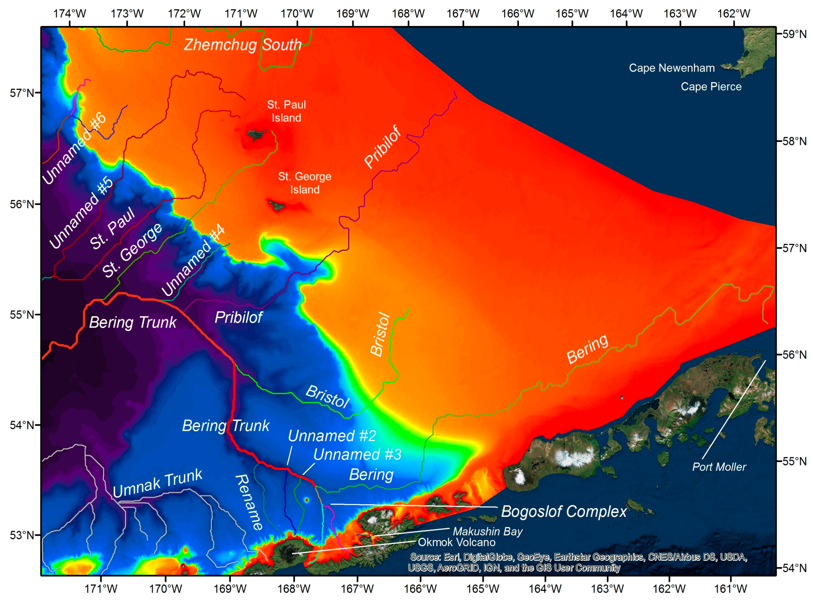
The Bering complex of canyons (Figure 7, Table 2) is to the northeast of the Umnak complex, and both NGA and GEBCO gazetteers place the Bering Canyon name label in a relatively deep area. There are 4 Bering complex canyons arrayed along 74 km of a deeper trunk, near the Bering label, extending south past Bogoslof Island and toward the Aleutian Islands. The NGA gazetteer names the westernmost canyon as Inanudak, and we suggest renaming this as we have shown that a canyon in the Umnak complex extends into Inanudak Bay of Umnak Island. The two middle canyons are unnamed but both end near Okmok volcano on Umnak Island. The fourth and easternmost of this group is labeled as Bogoslof Canyon by NGA at a location where our results show that West, East, and Trunk branches meet. Also, there is a disconnected Basin component in Makushin Bay, Unalaska Island. Therefore, we suggest that the Bogoslof Canyon name recognize these West, East, Trunk, and Basin divisions. The main thalweg of Bering extends for a distance of 771 km east of Bogoslof Canyon, ending just outside of Port Moller at a depth of 40 m. Bristol Canyon, named in both gazetteers, is much shorter (319 km) than Bering, extending onto the shelf only up to a depth 134 m and joining the Bering Trunk at a depth of 2920 m. The tributaries of both Bering Canyon and Pribilof Canyon cover most of the shelf, blocking the eastern reach of Bristol Canyon.
We expected that Pribilof Canyon would resolve into two main thalwegs due to the kidney shape of the canyon, but the southern thalweg is so long and drains such as large area, while the northern thalweg is so short and drains such a small area between the canyon and St. George Island, that we identify only the main thalweg. Several other relatively small canyons, some extending onto the shelf, join the Pribilof thalweg in deeper water (not shown). Since these join the Pribilof thalweg before joining the Bristol Canyon trunk, and none of them were named by GEBCO or NGA, we consider them all to be tributaries of Pribilof.
Just to the north of Pribilof Canyon is an unnamed, relatively short (111 km) canyon that joins the Bristol Trunk separately and is therefore potentially deserving of its own name (Unnamed#4). The next 3 canyons are all about equal in length (311–404 km) and depth range (<100 to >3500 m), also joining the Bering Trunk in deep water. The southern of the three drains the area between the Pribilof Islands, while the two others drain the area north of St Paul Island. The central canyon of the three was named St. George by the NGA gazetteer, and therefore we suggest changing it to St. Paul, and also suggest naming the southern unnamed canyon as St. George. The northern of the three canyons is Unnamed#5, and it merges with St. Paul to form a 150 km long trunk that extends to the Bering Trunk (not shown). Just to the north of Unnamed#5 is another canyon without a name (Unnamed#6), having two thalwegs that extend onto the shelf, and connecting with a trunk of 347 km to the Bering Trunk (not shown). Altogether, Bering Trunk and the canyons directly linked to it in our analysis drain an area of 329,961 km2.
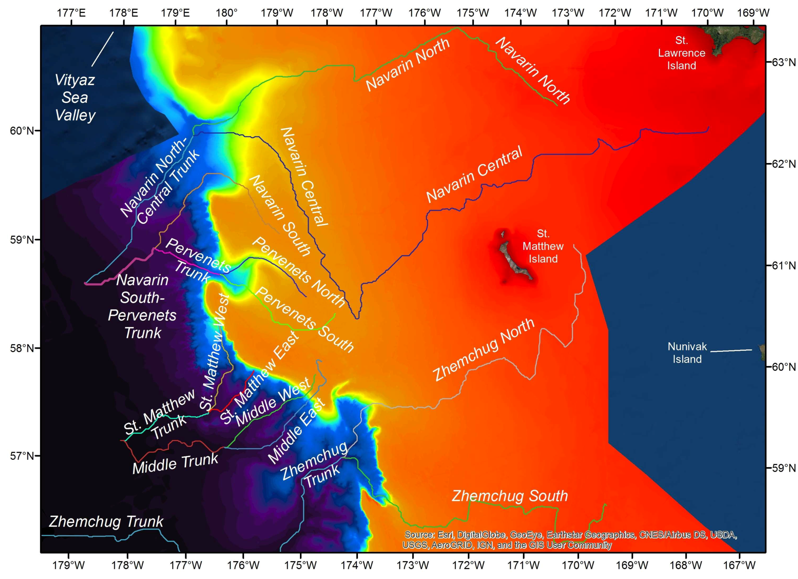
3.2.3. Navarin Canyon Thalwegs
The northern canyons (Figure 8, Table 3), which include Navarin, Pervents, St. Matthew, Middle, and Zhemchug, all have at least two main thalwegs. These canyons all eventually connect together in the deep water of the Aleutian Basin (not shown), but this is very poorly resolved in our compilation due to the disagreement between the GLORIA and smooth sheet depths. We derived three thalwegs from Navarin. The northern (551 km) and central (935 km) thalwegs are the longest, merging at a depth of 1698 m, well within the main body of the canyon, but the short southern (227 km) thalweg merges with the Pervenets Canyon trunk at a deep place (3356 m) between the canyons. This Navarin South-Pervenets Trunk then merges with the Navarin North-Central Trunk at a depth of 3679 m to form the Navarin Trunk. This was the only instance in our analysis where a thalweg from one canyon merged with a thalweg from another canyon rather than first merging with one of its own canyon thalwegs. Thus, it might be possible to consider South Navarin as a separate canyon from the North and Central Navarin thalwegs. Both the GEBCO (179°15′ E) and NGA labels (179°45′ E) for Navarin Canyon are too far to the west, and we suggest shifting them to 179°15′ W.
Pervenets Canyon has two relatively short thalwegs (North = 127 km and South = 172 km), as their reach onto the shelf is blocked by the south thalweg of Navarin Canyon. These Pervenets thalwegs join together at a depth of 821 m, near the edge of the canyon. Middle and St. Matthew Canyons do not have large, distinct incisions onto the shelf due to the South Pervenets and Central Navarin thalwegs. The East and West thalwegs of Middle and St. Matthew Canyons are both relatively short (<200 km), and they both join into trunks in deep water (3400–3600 m), far away from the shelf edge. Zhemchug Canyon has long northern (554 km) and southern (494 km) thalwegs, which join together near the edge of the canyon mouth, at a depth of 3021 m. Altogether, the Navarin area canyons drain an area of 632,670 km2; this value would increase if our deeper bathymetry were of sufficient resolution to connect them all.
3.3. Chart 16006 and the Zhemchug Canyon Pinnacles
There was no evidence in our bathymetry compilation of the Zhemchug pinnacles depicted on NOS Chart 16006. The warning circles (size range 21.0–32.2 km2) on Chart 16006 around each of these pinnacles overlapped nearly 17,000 corresponding soundings from our compilation (Table 4). The 8 fathom (14.6 m) pinnacle had 33 soundings from two cruises with a minimum depth of 147.9 m. The 13 fathom (23.8 m) and the 3.75 fathom (6.9 m) pinnacles occurred in relatively steep and deep places, with 3154 soundings from six cruises having a minimum depth of 463.7 m for the former, and 10,712 soundings from 11 cruises having a minimum depth of 224.0 m for the latter. The fourth pinnacle, of unknown depth, had 2756 soundings from 13 cruises with a minimum depth of 137.2 m.
3.4. Canyon Thalwegs and Other Seafloor Features
Our canyon designations generally agreed with those of [14] but did have some differences worth noting. The main difference was in thalweg length, with those of [14] shorter at both the shallow and deep ends, owing to differences in methods. Harris and Whiteway [14] defined their thalwegs based on significant deflections in 100 m depth contours, while our thalwegs were based on the ArcMap Hydrology function (minimum lower limit needed to drain 1000 upstream cells), and canyon designations were mostly based on those canyons named in the NGA and GEBCO gazetteers. Thus, we have fewer canyons composed of numerous connected thalwegs that extend farther onto the shelf and farther into the Aleutian Basin, while [14] has more numerous, shorter canyons generally restricted just to the slope area. We did identify some canyons that [14] did not, such as Korovin, Unnamed#1, and Herbert in the Umnak complex and Unnamed#3 in the Bering complex.
We did not divide our bathymetry surface into geomorphic provinces, but our surface differed significantly from the geomorphic features of the EBS shelf [15]. Most of the EBS shelf was interrupted by three classes of relief (low, medium, and high) [15], while our compilation did not have much relief on the shelf at all. Nor do we have the shelf valleys or basins perched on the shelf. We hypothesize that these features are all most likely to have come from bathymetry errors. The linear “medium” shelf relief features that extend north from Unimak Pass to Nome are most likely vessel paths. The “basin perched on shelf” and “Moderate size shelf valley” just to the north of Navarin Canyon are most likely derived from errant, shallow depths. Our bathymetry has some discontinuous features in this area and could use more soundings for clarification.
3.5. Other Compilations
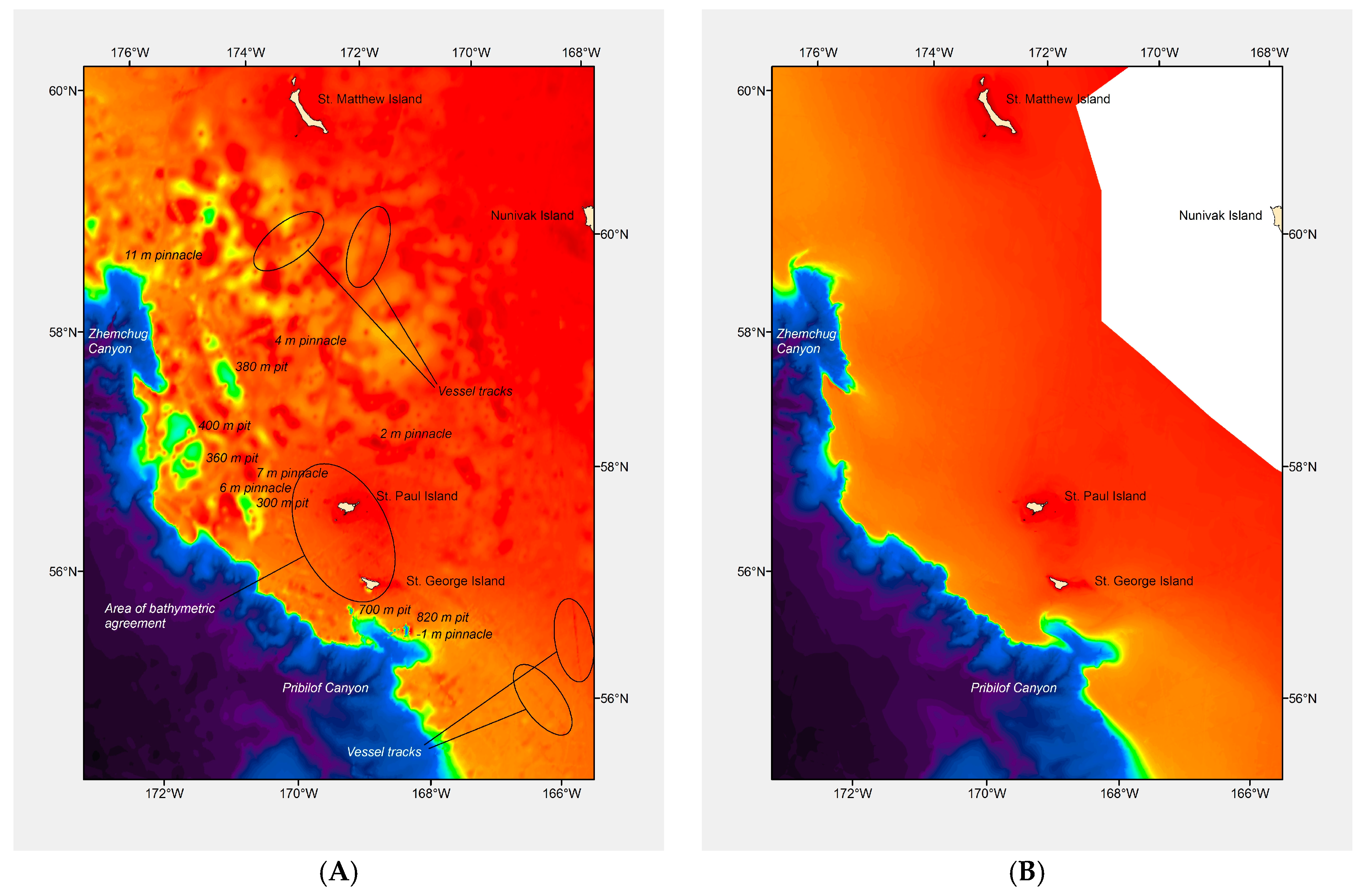
The global [9,10,11] and AKRO 2005 compilations were very similar to each other. These were also generally similar to our compilation in the area around the Pribilof Islands and southern EBS shelf, corresponding to an area covered by smooth sheets and the 1970 Rainier cruise, and they were generally similar to our compilation in the Aleutian Basin and EBS slope canyons. Beyond these areas of agreement, these compilations had numerous hills and pits, especially along the shelf edge near the canyons, where our compilation is relatively flat. For example, in the GEBCO compilation [11], pits just south of Zhemchug Canyon exceeded 400 m in depth (Figure 9A) in areas we characterize as about 120 m deep (Figure 9B). ETOPO1 [10] had a pit almost 700 m deep and about 100 km wide just inshore of Navarin Canyon, an area we estimate to be about 100 to 200 m deep. All also had some smaller pits along the rim of Pribilof Canyon; one in the GEBCO compilation [11] exceeded 800 m and was surrounded by depths equivalent to the sea surface (Figure 9A), all in an area we characterize as about 140 to 160 m deep (Figure 9B). These compilations also had straight lines, presumably from underway files from vessel transects, both shallower and deeper than surrounding areas; these created significant ridges and narrow canyons (Figure 9A). As mentioned previously, the AKRO compilation of 2005 also had several shallow spots, regarded as pinnacles, near the Zhemchug Canyon area.
The AKRO 2017 and ARDEM [13] compilations are the most recent published for this area. The AKRO 2017 compilation has much in common with the previous compilations, such as numerous pinnacles and pits along with numerous visible ship tracks. Within Zhemchug Canyon there is a pit >3000 m in depth in an area we show is about half of that depth. Between Zhemchug Canyon and the Pribilofs there are some large pits extending down to about 300 and 400 m deep—all areas we have as being ~100 to 120 m deep. South of Zhemchug there are two groups of some very small pits; the northern group is as deep as ~3200 m in areas of the shelf that we have as ~200 to 600 m, while the southern group is as deep as ~3400 m in an area we have as ~140 to 150 m deep. The ARDEM compilation greatly reduced the appearance of deep hills and valleys on the EBS shelf that were so visible in the other compilations and in the geomorphic provinces of [15]. We presume that the improvement comes from avoidance of satellite-derived bathymetry. This depiction of the area, specifically the EBS shelf, corresponds to our AFSC cruises in this area: no pinnacles, no pits or hills, and no slender ridges or canyons. Our mid-water acoustic surveys for pollock provide a continuous record of the seafloor and show kilometer after kilometer of flat seafloor on the EBS shelf. Our bottom trawl surveys test the slope and rugosity of the seafloor by dragging nets on it. The EBS shelf bottom trawl survey is our only trawl survey in which the fishing captain of our chartered survey vessels can simply drop the net to the seafloor and drag it in any direction for 30 min without risk of tears or hangs, because the seafloor is so smooth and so well-covered with unconsolidated sediments. The AFSC’s other current bottom trawl surveys, such as in the GOA, AI, the EBS slope, and our historical surveys in the US west coast shelf and slope, all require significant searching and planning for obtaining successful bottom tows without incurring damage to the net. Still, ARDEM [13] has several shallow outliers that appear as pinnacles in Navarin Canyon, and in other places just above and just below the shelf break. We trace some of these features to soundings from very small scale charts that probably could be excluded from the ARDEM compilation [13] without the loss of any information.
4. Discussion
This EBS slope 100 m resolution bathymetry compilation is our latest regional seafloor map of Alaska. Soon, we expect to publish similar compilations for the western Gulf of Alaska and the eastern Gulf of Alaska. Together, these new data sets, along with our previously published data sets, will create a continuous 100 m resolution surface of the Alaska seafloor ranging from Dixon Entrance in the southwest to Stalemate Bank in the west and to the Bering Strait in the north (Figure 1). These data are already being incorporated into the global lower resolution GEBCO map [11] and may also serve as an extension of a new, higher resolution version of IBCAO [12], providing a bridge from the Arctic into the North Pacific for one of Regional Data Assembly and Coordination Centers (RDACCs) of the Nippon Foundation—GEBCO Seabed 2030 Project [48]. Due to the general agreement of the ARDEM [13] regional bathymetry and our EBS slope compilation, we propose that combining data sources, especially with the Russian navigational charts, would result in an improved coverage across the entire Bering Sea. The Interferometric Synthetic Aperture Radar (ifsar) 5 m Digital Elevation Model of Alaska is in progress (http://ifsar.gina.alaska.edu/) and would serve as an excellent source for those areas above sea level.
4.1. Data Quality
With our heavy reliance on non-hydrographic underway files from numerous sources, on older data sets, and on a paucity of multibeam data, there is substantial room for improvement in our compilation. The large area of the Aleutian Basin in our map could simply and easily be improved by developing an appropriate correction between the smooth sheet and GLORIA underway files that are the only information for that area. A Gulf of Mexico bathymetry compilation covering a similar depth range was constructed entirely out of high-quality 3-D seismic data, allowing a 40 ft (12.2 m) pixel size [49], which represents a 67-fold increase in resolution over our 100 m pixel size. We did not have any high-quality 3-D seismic data for our project area, and it was nearly three times the size of the Gulf of Mexico compilation. Any dedicated bathymetry cruises in the EBS slope area, especially those that range across the steepest portion of the slope, would be a valuable addition to future versions. Lack of bathymetry data, or reliance on inaccurate bathymetry data, produces depth maps with large errors or uncertainties. If utilized, these low quality maps perpetuate their errors into plans for research cruises, survey strata boundaries, station placement, physical and biological analyses, and conclusions about management of resources in the area. Many of the bathymetry errors we noted in the regional and global compilations even occur in the global background map provided by our ArcMap software (ESRI), which we used in our figures. Better bathymetry can be a useful guide for better ocean science.
4.2. Data Editing
Visualizing and editing the data were the most important and extensive parts of creating this bathymetry surface and these canyon thalwegs. We rely on extended color ramps and utilizing very narrow color bands for distinguishing differences between neighboring depths. Slope surfaces of TINs emphasize depth differences in the raw point data and lead to most of the outliers that we investigate for correction or deletion. Since we were interested in describing the canyons in this EBS slope regional bathymetry compilation, the processing required additional steps of creating aspect surfaces and thalwegs. This, in turn, led to additional rounds of editing, as we created vertical depth corrections for individual cruises in an attempt to keep the thalwegs from following individual cruise tracks. We have used these methods as a means of working with lower quality data sets and as a substitute for automated outlier detection algorithms.
4.3. Gazetteer Names
We tried to align our canyon thalwegs with previously published canyon names, but our results indicated numerous differences. Six of our canyons are unnamed, and we suggested several name changes due to differences between our thalweg paths and the locations of source names, such as islands. For example, Okmuk Canyon of the NGA gazetteer did not appear to exist in our analysis, but this name might be re-used for one of the other unnamed canyons in the area. The Inanudak Canyon label of the NGA gazetteer was used for a canyon that extends to Okmok Volcano, not Inanudak Bay. We hope to work with GEBCO’s Sub-Committee on Undersea Feature Names (SCUFN: https://www.gebco.net/about_us/committees_and_groups/) to update the canyon names in our study area.
4.4. Pinnacles
Our lack of finding the pinnacles was worrisome, as they pose a significant navigational danger, but not completely unexpected. The four Zhemchug pinnacles do not show up on global compilations such as [9], ETOPO1 [10], and GEBCO [11], nor on regional bathymetry compilations such as the AKRO of 2005, ARDEM [13], and the AKRO of 2017. The 1986 GLORIA cruise also did not reveal any pinnacles within Zhemchug canyon. Despite not confirming the four Zhemchug pinnacles from NOS Chart 16006, the 2005 AKRO bathymetry compilation depicted three new pinnacles to the east of Zhemchug Canyon and five new pinnacles south of the canyon and west of St. Paul Island. While exploring Pribilof and Zhemchug Canyons with a Deep-Worker mini-submersible and an ROV in 2007 [34], researchers on the MV Esperanza led an unsuccessful effort to find and document the four NOS Chart 16006 pinnacles and the eight 2005 AKRO pinnacles [pers. comm. John Hocevar 2017].
A potential source of the pinnacles might be the nearby seafloor feature of St. Paul Spur, which was mapped partially with singlebeam on two AFSC cruises [44]. These AFSC cruises clearly defined two ridges, both of which rise only to a depth of about 85 m [44], which is not much different than the depths reported on smooth sheet H08103, and are too shallow to be candidates for the reports of pinnacles. However, a primary finding of [44] acoustic analysis on the Zhemchug Canyon ridges was that extremely dense schools of juvenile Pacific ocean perch (Sebastes alutus) and northern rockfish (S. polyspinus) rise off the seafloor during daylight hours [44] (see Figure 8). We propose that these fish, which are good backscatter targets, are the source of the reports of pinnacles in this area. An additional cruise on the MV Esperanza exploring Zhemchug and Pribilof canyons was conducted in 2012 [35]: once again, no pinnacles were found, but no time was devoted to the search [pers. comm. John Hocevar, 2017].
Since dozens of AFSC cruises have passed through this Zhemchug area and none of them have encountered the pinnacles, we suggest that the status of the pinnacles be changed from legendary to mythical.
Supplementary Materials
The following are available online at https://zenodo.org/record/3247187#.XQicNaIRVPZ, Thalwegs.zip: a zipped ArcMap shape file of the thalweg polylines, and EBS Slope Bathymetry.zip, a zipped file of bathymetry image and world file for plotting as a backdrop to the thalwegs.
Author Contributions
M.Z. was the primary author of this document; M.Z. and M.M.P. both extracted, formatted, and edited bathmetry data, M.M.P. mostly extracted the comparative data and did the digitizing, and both participated in the thalweg creation.
Acknowledgments
Thanks to Wayne Palsson, Jodi Pirtle, Jennifer Jencks, Michael Martin, and H. Gary Greene for helpful reviews of the manuscript. The staff at NGDC (National Geophysical Data Center (Boulder, CO, USA): http://www.ngdc.noaa.gov) provided frequent assistance with smooth sheets and multibeam data sets. Doug Graham and Maryellen Sault helped with National Geodetic Survey shoreline products (NOAA Shoreline Explorer web site: http://www.ngs.noaa.gov/NSDE/). The staff at Pacific Hydrographic Branch, Office of Coast Survey, National Ocean Service, assisted with multibeam survey products. Abigail McCarthy and Scott R. Furnish assisted with accessing and understanding the MACE acoustic data (https://data.noaa.gov/dataset). Frank Parker and Tara Wallace helped with Notice to Mariner reports about the Zhemchug pinnacles and Robert Akro (Lamont-Doherty Earth Observatory, Columbia University, New York, NY, USA) supplied Alpha Helix data. Jerry Hoff helped with EBS slope bottom trawl cruises and Miller Freeman 200712. David Doyle (Base 9 Geodetic Consulting Services, formerly NGS) and David Grosh (NOS) provided key assistance with St. Matthew Island smooth sheet georegistration. Underway data from the BEST cruises were provided by NCAR/EOL (http://data.eol.ucar.edu/) under sponsorship of the National Science Foundation. The GEBCO bathymetry data were supplied by data request through the British Oceanographic Data Center (Liverpool, UK) (https://www.bodc.ac.uk). Funding for much of the work was provided by NOAA’s Essential Fish Habitat (EFH), Habitat and Ecological Processes Research (HEPR) through the NMFS Alaska Regional Office. The findings and conclusions in the paper are those of the authors and do not necessarily represent the views of the National Marine Fisheries Service, NOAA. Reference to trade names does not imply endorsement by the National Marine Fisheries Service, NOAA. Otherwise we received no funds for covering the costs to publish in open access.
Conflicts of Interest
The authors declare no conflict of interest. The founding sponsors had no role in the design of the study; in the collection, analyses, or interpretation of data; in the writing of the manuscript; or in the decision to publish the results.
References
- Normark, W.R.; Carlson, P.R. Giant submarine canyons: Is size any clue to their importance in the rock record. In Extreme Depositional Environments; Chan, M.A., Archer, A.W., Eds.; Geological Society of America: Boulder, CO, USA, 2003. [Google Scholar]
- Hawley, J.H. Hydrographic Manual; U.S. Department of Commerce, U.S. Coast and Geodetic Survey, Special Publication No. 143; U.S. Government Printing Office: Washington, DC, USA, 1931.
- Zimmermann, M.; Prescott, M.M.; Rooper, C.N. Smooth Sheet Bathymetry of the Aleutian Islands; U.S. Department Commerce: Washington, DC, USA, 2013.
- Carlson, P.R.; Karl, H.A. Discovery of two new large submarine canyons in the Bering Sea. Mar. Geol. 1984, 56, 159–179. [Google Scholar] [CrossRef]
- Carlson, P.R.; Karl, H.A. High-Resolution Seismic Reflection Profiles: Navarin Basin Province, Northern Bering Sea; U.S. Geological Survey: Washington, DC, USA, 1981.
- Carlson, P.R.; Karl, H.A. High-Resolution Seismic Reflection Profiles Collected in 1981 in Navarin Basin Province, Bering Sea; U.S. Geological Survey: Washington, DC, USA, 1982.
- Fischer, J.M.; Carlson, P.R.; Karl, H.A. Bathymetric Map of Navarin Basin Province, Northern Bering Sea; U.S. Geological Survey: Washington, DC, USA, 1982.
- Jones, E.L. Safeguard the Gateways of Alaska: Her Waterways; U.S. Department of Commerce, U.S. Coast and Geodetic Survey, Special Publication No. 50; U.S. Government Printing Office: Washington, DC, USA, 1918.
- Smith, W.H.F.; Sandwell, D.T. Global seafloor topography from satellite altimetry and ship depth soundings. Science 1997, 277, 1957–1962. [Google Scholar] [CrossRef]
- Amante, C.; Eakins, B.W. ETOPO1 1 Arc-Minute Global Relief Model: Procedures, Data Sources and Analysis. In NOAA Technical Memorandum ESDIS NGDC-24; NOAA: Silver Spring, MD, USA, 2009. [Google Scholar]
- Weatherall, P.; Marks, K.M.; Jakobsson, M.; Schmitt, T.; Tani, S.; Arndt, J.E.; Rovere, M.; Chayes, D.; Ferrini, V.; Wigley, R. A new digital bathymetric model of the world’s oceans. Earth Space Sci. 2015, 2, 331–345. [Google Scholar] [CrossRef]
- Jakobsson, M.; Mayer, L.; Coakley, B.; Dowdeswell, J.A.; Forbes, S.; Fridman, B.; Hodnesdal, H.; Noormets, R.; Pedersen, R.; Rebesco, M.; et al. The International Bathymetric Chart of the Arctic Ocean (IBCAO); Version 3.0; John Wiley & Sons, Inc.: Hoboken, NJ, USA, 2012. [Google Scholar]
- Danielson, S.L.; Dobbins, E.L.; Jakobsson, M.; Johnson, M.A.; Weingartner, T.J.; Williams, W.J.; Zarayskaya, Y. Sounding the northern seas. Eos 2015, 96. [Google Scholar] [CrossRef]
- Harris, P.T.; Whiteway, T. Global distribution of large submarine canyons: Geomorphic differences between active and passive continental margins. Mar. Geol. 2011, 285, 69–86. [Google Scholar] [CrossRef]
- Harris, P.T.; Macmillan-Lawler, M.; Rupp, J.; Baker, E.K. Geomorphology of the oceans. Mar. Geol. 2014, 352, 4–24. [Google Scholar] [CrossRef]
- Zimmermann, M.; Prescott, M.M. Smooth Sheet Bathymetry of Cook Inlet, Alaska; U.S. Department Commerce: Washington, DC, USA, 2014.
- Prescott, M.M.; Zimmermann, M. Smooth Sheet Bathymetry of Norton Sound; U.S. Department Commerce: Washington, DC, USA, 2015.
- Zimmermann, M.; Prescott, M.M. Smooth Sheet Bathymetry of the Central Gulf of Alaska; U.S. Department Commerce: Washington, DC, USA, 2015.
- Nichol, D.G.; Kotwicki, S.; Zimmermann, M. Diel vertical migration of adult Pacific cod Gadus macrocephalus in Alaska. J. Fish Biol. 2013, 83, 170–189. [Google Scholar] [CrossRef] [PubMed]
- Rooper, C.N.; Zimmermann, M.; Prescott, M.M.; Hermann, A.J. Predictive models of coral and sponge distribution, abundance and diversity in bottom trawl surveys of the Aleutian Islands, Alaska. Mar. Ecol. Prog. Ser. 2014, 503, 157–176. [Google Scholar] [CrossRef]
- Rooper, C.N.; Zimmermann, M.; Prescott, M.M. Comparison of modeling methods to predict the spatial distribution of deep-sea coral and sponge in the Gulf of Alaska. Deep Sea Res. Part I Oceanogr. Res. Pap. 2017, 126, 148–161. [Google Scholar] [CrossRef]
- Zimmermann, M.; Reid, J.A.; Golden, N. Using smooth sheets to describe groundfish habitat in Alaskan waters. Deep Sea Res. II Top. Stud. Oceanogr. 2016, 132, 210–226. [Google Scholar] [CrossRef]
- Zimmermann, M. Comparison of the physical attributes of the central and eastern Gulf of Alaska IERP inshore study sites. Deep Sea Res. II Top. Stud. Oceanogr. 2018, in press. [Google Scholar]
- Zimmermann, M.; De Robertis, A.; Ormseth, O. Verification of historical smooth sheet bathymetry. Deep Sea Res. II Top. Stud. Oceanogr. 2018. submitted for publication. [Google Scholar]
- Mordy, C.W.; Stabeno, P.J.; Kachel, N.B.; Kachel, D.; Ladd, C.; Zimmermann, M.; Doyle, M. Importance of canyons to the northern gulf of Alaska ecosystem. Deep Sea Res. II Top. Stud. Oceanogr. 2018. submitted for publication. [Google Scholar]
- Zimmermann, M.; Ruggerone, G.T.; Freymueller, J.T.; Kinsman, N.; Ward, D.H.; Hogrefe, K. Volcanic ash deposition, eelgrass beds, and inshore habitat loss from the 1920s to the 1990s at Chignik, Alaska. Estuar. Coast. Shelf. Sci. 2018, 202, 69–86. [Google Scholar] [CrossRef]
- Laman, E.A.; Rooper, C.N.; Rooney, S.C.; Turner, K.A.; Cooper, D.W.; Zimmermann, M. Model-Based Essential Fish Habitat Definitions for Bering Sea Groundfish Species; U.S. Department Commerce: Washington, DC, USA, 2017.
- Rooney, S.; Rooper, C.N.; Laman, E.A.; Turner, K.; Cooper, D.; Zimmermann, M. Model-Based Essential Fish Habitat Definitions for Gulf of Alaska Groundfish Species; U.S. Department Commerce: Washington, DC, USA, 2018.
- Laman, E.A.; Rooper, C.N.; Turner, K.; Rooney, S.; Cooper, D.; Zimmermann, M. Using species distribution models to define essential fish habitat in Alaska. Can. J. Fish. Aquat. Sci. 2017. [Google Scholar] [CrossRef]
- Turner, K.; Rooper, C.N.; Laman, E.A.; Rooney, S.C.; Cooper, D.W.; Zimmermann, M. Model-Based Essential Fish Habitat Definitions for Aleutian Island Groundfish Species; U.S. Department Commerce: Washington, DC, USA, 2017.
- Pirtle, J.; Shotwell, S.K.; Zimmermann, M.; Reid, J.A.; Golden, N. Habitat Suitability Models for Groundfish in the Gulf of Alaska. Deep Sea Res. II Top. Stud. Oceanogr. 2017, in press. [Google Scholar] [CrossRef]
- McGowan, D.W.; Horne, J.K.; Thorson, J.T.; Zimmermann, M. Influence of environmental factors on capelin distributions in the Gulf of Alaska. Deep Sea Res. II Top. Stud Oceanogr. 2017, in press. [Google Scholar] [CrossRef]
- Food and Agriculture Organization. The state of world fisheries and aquaculture 2016. In Contributing to Food Security and Nutrition for All; FAO: Rome, Italy, 2016. [Google Scholar]
- Miller, R.J.; Hocevar, J.; Stone, R.P.; Fedorov, D.V. Structure-forming corals and sponges and their use as fish habitat in Bering Sea submarine canyons. PLoS ONE 2012, 7. [Google Scholar] [CrossRef] [PubMed]
- Miller, R.J.; Juska, C.; Hocevar, J. Submarine canyons as coral and sponge habitat on the eastern Bering Sea. Glob. Ecol. Conserv. 2015, 4, 85–90. [Google Scholar] [CrossRef]
- Sigler, M.F.; Rooper, C.N.; Hoff, G.R.; Stone, R.P.; McConnaughey, R.A.; Wilderbuer, T.K. Faunal features of submarine canyons on the eastern Bering Sea slope. Mar. Ecol. Prog. Ser. 2015, 526, 21–40. [Google Scholar] [CrossRef]
- Hoff, G.R. Identification of skate nursery habitat in the eastern Bering Sea. Mar. Ecol. Prog. Ser. 2010, 403, 243–254. [Google Scholar] [CrossRef]
- Hoff, G.R. Results of the 2012 Eastern Bering Sea Upper Continental Slope Survey of Groundfish and Invertebrate Resources; U.S. Department of Commerce: Washington, DC, USA, 2013.
- Nghiem, S.V.; Clemete-Colon, P.; Rigor, I.G.; Hall, D.K.; Neumann, G. Seafloor control on sea ice. Deep Sea Res. Part II Top. Stud. Oceanogr. 2012, 77–80, 52–61. [Google Scholar] [CrossRef]
- Springer, A.M.; McRoy, C.P.; Flint, M.V. The Bering Sea green belt: Shelf-edge processes and ecosystem production. Fish. Oceanogr. 1996, 5, 205–223. [Google Scholar] [CrossRef]
- Wong, S.N.P.; Gjerdrum, C.; Morgan, K.H.; Mallory, M.L. Hotspots in cold seas: The composition, distribution, and abundance of marine birds in the North American Arctic. J. Geophys. Res. Oceans 2014, 119, 1691–1705. [Google Scholar] [CrossRef]
- Wong, A.M.; Campagnoli, J.G.; Cole, M.A. Assessing 155 years of hydrographic survey data for high resolution bathymetry grids. In Proceedings of the Oceans 2007, Vancouver, BC, Canada, 29 September–4 October 2007. [Google Scholar]
- Zimmermann, M.; Benson, J. Smooth Sheets: How to Work with Them in a GIS to Derive Bathymetry, Features and Substrates; U.S. Department Commerce: Washington, DC, USA, 2013.
- Rooper, C.N.; Hoff, G.R.; De Robertis, A. Assessing habitat utilization and rockfish (Sebastes spp.) biomass on an isolated rocky ridge using acoustics and stereo image analysis. Can. J. Fish. Aquat. Sci. 2010, 67, 1658–1670. [Google Scholar] [CrossRef]
- McKelvey, D.; Steinessen, S. Results of the March 2014 Acoustic-Trawl Survey of Walleye Pollock (Gadus chalcogrammus) Conducted in the Southeastern Aleutian Basin Near Bogoslof Island, Cruise DY2014–02; NOAA: Silver Spring, MD, USA, 2015.
- Honkalehto, T.; McCarthy, A. Results of the Acoustic-Trawl Survey of Walleye Pollock (Gadus Chalcogrammus) on the U.S. and Russian Bering Sea Shelf in June–August 2014 (DY1407); NOAA: Silver Spring, MD, USA, 2015.
- Carter, D.J.T. Echo-Sounding Correction Tables, 3rd ed.; Hydrographic Department Ministry of Defence: Taunton, UK, 1980.
- Mayer, L.; Jakobsson, M.; Allen, G.; Dorschel, B.; Falconer, R.; Ferrini, V.; Lamarche, G.; Snaith, H.; Weatherall, P. The Nippon Foundation—GEBCO seabed 2030 project: The quest to see the world’s oceans completely mapped by 2030. Geosciences 2018, 8. [Google Scholar] [CrossRef]
- Kramer, K.V.; Shedd, W.W. A 1.4-billion-pixel map of the Gulf of Mexico seafloor. Eos 2017, 98. [Google Scholar] [CrossRef]
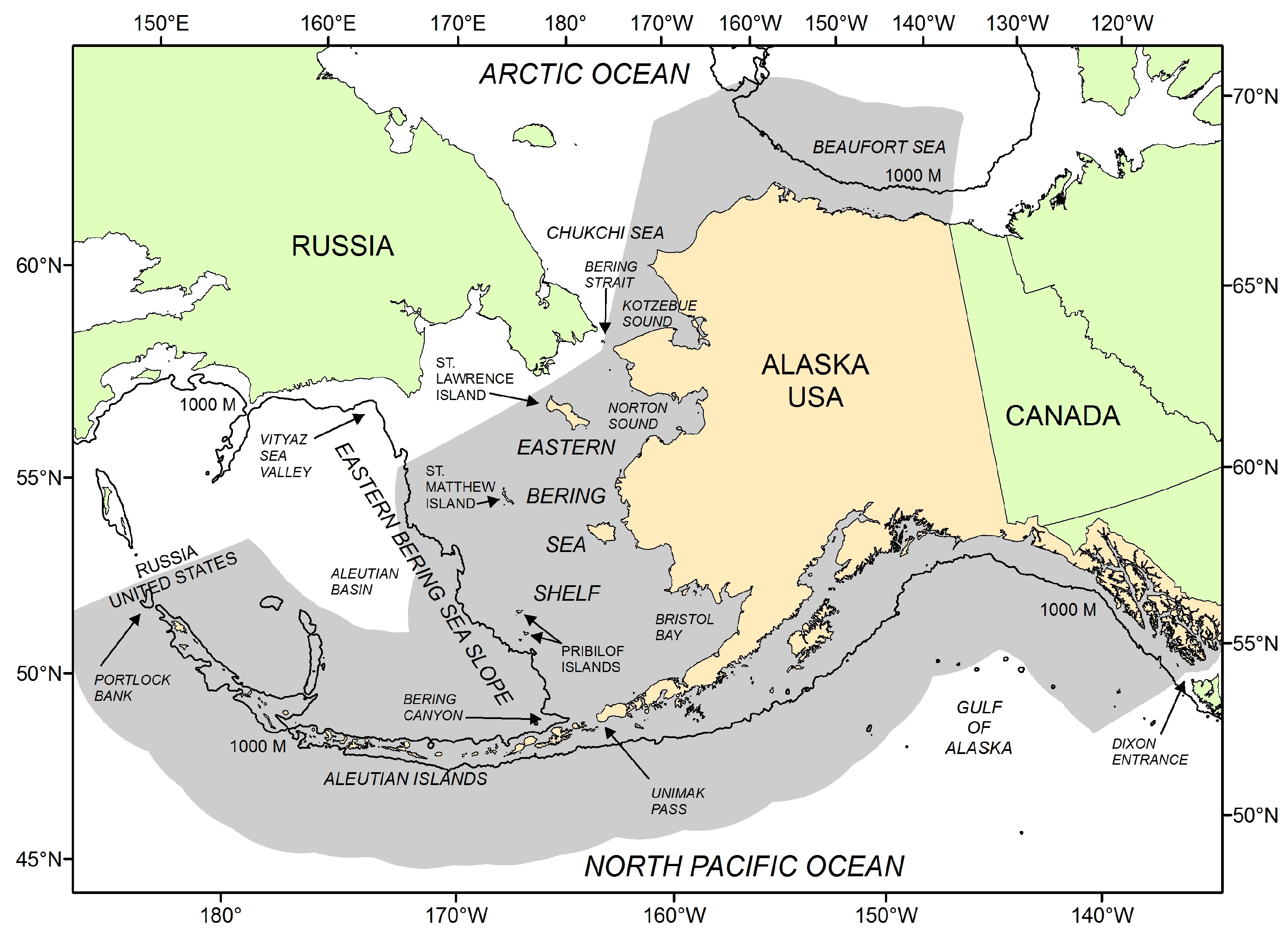
Figure 1.
Overview map of the study area, with the US Exclusive Economic Zone in gray.

Figure 2.
NOS navigational Chart 9302 from 1948. Eastern Bering Sea slope canyons are poorly defined by dashed lines for the 100 (traced in red) and 1000 (traced in black) fathom depth contours. This chart was replaced by Chart 16006 in 1975.
Figure 2.
NOS navigational Chart 9302 from 1948. Eastern Bering Sea slope canyons are poorly defined by dashed lines for the 100 (traced in red) and 1000 (traced in black) fathom depth contours. This chart was replaced by Chart 16006 in 1975.

Figure 3.
Detail of NOS navigational chart 16006 (Edition 37, 2015, Scale 1:1,534,076), showing reported pinnacles in the Zhemchug Canyon area.
Figure 3.
Detail of NOS navigational chart 16006 (Edition 37, 2015, Scale 1:1,534,076), showing reported pinnacles in the Zhemchug Canyon area.

Figure 4.
Sources of bathymetry data used in this EBS slope compilation.

Figure 5.
Bathymetry of the eastern Bering Sea slope.

Figure 6.
Thalwegs of the Umnak Canyon area of the eastern Bering Sea slope.

Figure 7.
Thalwegs of the Bering Canyon area of the eastern Bering Sea slope.

Figure 8.
Thalwegs of the Navarin Canyon area of the eastern Bering Sea slope.

Figure 9.
Comparison of eastern Bering Sea bathymetry between (A) the global GEBCO compilation [11] with numerous artifacts in the area between Zhemchug and Pribilof canyons and (B) our bathymetry which depicts a much smoother surface.
Figure 9.
Comparison of eastern Bering Sea bathymetry between (A) the global GEBCO compilation [11] with numerous artifacts in the area between Zhemchug and Pribilof canyons and (B) our bathymetry which depicts a much smoother surface.


Table 1.
Umnak Canyon names and metrics described from west to east.
| Canyon | Area Drained km2 | Start Depth m | End Depth m | Mean Slope Degrees | Thalweg Length km |
|---|---|---|---|---|---|
| Korovin | 611 | 686 | 3511 | 3.8 | 71 |
| Atka Complex | 2418 | 935 | 3512 | 3.4 | 132 |
| Trunk | 543 | 3305 | 3512 | 0.7 | 26 |
| West | 737 | 1015 | 3303 | 4.2 | 51 |
| East | 1138 | 935 | 3304 | 3.8 | 55 |
| Amlia Complex | 7102 | 112 | 3714 | 1.9 | 281 |
| Thalweg | 4549 | 1064 | 3714 | 2.1 | 210 |
| Basin Thalweg | 2553 | 112 | 1034 | 1.6 | 72 |
| Unnamed#1 | 3700 | 842 | 3698 | 1.6 | 156 |
| Seguam Complex | 5597 | 170 | 3555 | 2.6 | 235 |
| Trunk | 1563 | 2462 | 3555 | 1.6 | 56 |
| West | 1496 | 170 | 2460 | 3.4 | 79 |
| East | 674 | 558 | 2462 | 3.0 | 56 |
| Basin Thalweg | 1864 | 565 | 558 | 1.2 | 43 |
| Amukta | 3570 | 270 | 2945 | 3.6 | 119 |
| Chagulak | 1222 | 376 | 2936 | 3.8 | 67 |
| Amuk.-Chag. Trunk (includes drainage of both canyons) | 5871 | 2942 | 3295 | 1.8 | 60 |
| Yunaska | 4124 | 163 | 2789 | 2.4 | 121 |
| Herbert | 374 | 1563 | 2789 | 4.6 | 57 |
| Herb.-Yun. Trunk (includes drainage of both canyons) | 4821 | 2789 | 2712 | 0.9 | 6 |
| Carlisle | 1944 | 892 | 2713 | 4.1 | 101 |
| Umnak | 4810 | 422 | 2444 | 4.4 | 126 |
| Umnak Trunk (includes all drainage except Korovin and Atka) | 56,385 | 2445 | 3713 | 1.8 | 453 |
| Inanudak | 2352 | 71 | 2453 | 4.2 | 121 |
Table 2.
Bering Canyon names and metrics described from south to north.
| Canyon | Area Drained km2 | Start Depth m | End Depth m | Mean Slope Degrees | Thalweg Length km |
|---|---|---|---|---|---|
| Rename | 2536 | 560 | 2601 | 2.7 | 98 |
| Unnamed#2 | 1117 | 558 | 2460 | 2.4 | 77 |
| Unnamed#3 | 806 | 893 | 2312 | 2.0 | 67 |
| Bogoslof Complex | 3192 | 34 | 2194 | 3.0 | 183 |
| Trunk | 669 | 1899 | 2194 | 1.6 | 21 |
| West | 1053 | 106 | 1897 | 3.2 | 73 |
| East | 1471 | 56 | 1897 | 2.8 | 71 |
| Basin Thalweg | 208 | 34 | 215 | 4.3 | 18 |
| Bering Thalweg | 97,547 | 40 | 2193 | 0.4 | 771 |
| Bering Trunk (includes all drainage) | 329,961 | 2192 | 3694 | 0.9 | 696 |
| Bristol | 20,019 | 134 | 2920 | 1.0 | 319 |
| Pribilof | 74,422 | 61 | 3334 | 0.7 | 529 |
| Unnamed#4 | 2375 | 128 | 3352 | 2.4 | 111 |
| St George | 9971 | 46 | 3468 | 1.0 | 311 |
| St Paul | 15,025 | 70 | 3522 | 0.8 | 360 |
| Unnamed#5 | 11,634 | 73 | 3522 | 0.9 | 404 |
| St P.-Un.#5 Trunk (includes drainage from both canyons) | 33,485 | 3522 | 3629 | 0.3 | 150 |
| Unnamed#6 Complex | 9712 | 115 | 3694 | 1.5 | 511 |
| Trunk | 6325 | 1533 | 3694 | 0.8 | 347 |
| North | 1454 | 124 | 1524 | 3.7 | 58 |
| South | 1932 | 115 | 1541 | 1.5 | 106 |
Table 3.
Navarin Canyon names and metrics described from south to north.
| Canyon | Area Drained km2 | Start Depth m | End Depth m | Mean Slope Degrees | Thalweg Length km |
|---|---|---|---|---|---|
| Zhemchug Complex | 428,642 | 64 | 3810 | 0.9 | 1548 |
| Trunk | 345,451 | 3021 | 3810 | 0.6 | 500 |
| North | 50,833 | 64 | 3013 | 0.9 | 554 |
| South | 32,359 | 68 | 3022 | 1.1 | 494 |
| Middle Complex | 23,242 | 131 | 3743 | 1.3 | 498 |
| Trunk | 12,028 | 3589 | 3743 | 0.2 | 162 |
| West | 5544 | 133 | 3589 | 2.1 | 146 |
| East | 5670 | 131 | 3589 | 1.6 | 190 |
| St Matthew Complex | 10,340 | 138 | 3743 | 2.3 | 346 |
| Trunk | 5232 | 3465 | 3743 | 0.4 | 124 |
| West | 3414 | 138 | 3464 | 3.0 | 142 |
| East | 1693 | 645 | 3464 | 3.7 | 81 |
| Pervenets Complex | 17,507 | 136 | 3365 | 0.7 | 387 |
| Trunk | 5945 | 821 | 3365 | 2.2 | 88 |
| North | 4442 | 136 | 819 | 0.4 | 127 |
| South | 7121 | 137 | 819 | 0.3 | 172 |
| Navarin Complex | 152,940 | 38 | 3680 | 0.4 | 2054 |
| North | 37,638 | 56 | 1691 | 0.3 | 551 |
| Central | 97,765 | 38 | 1695 | 0.2 | 935 |
| Nav. N.-Cent. Trunk | 5652 | 1698 | 3680 | 0.9 | 227 |
| South | 7483 | 138 | 3363 | 1.5 | 241 |
| Nav. S.-Perv. Trunk (not including Pervenets drainage) | 4401 | 3356 | 3679 | 0.2 | 99 |
Table 4.
We summarized the soundings from numerous different cruises used for our compilation at four sites near Zhemchug Canyon where pinnacles are reported as potential navigational hazards on NOS navigational Chart 16006.
Table 4.
We summarized the soundings from numerous different cruises used for our compilation at four sites near Zhemchug Canyon where pinnacles are reported as potential navigational hazards on NOS navigational Chart 16006.
| Pinnacle | Reported by | Year Reported | Depth in Meters | Number of Cruises | Depth Mean (m) | Depth Range (m) | Soundings (n) |
|---|---|---|---|---|---|---|---|
| 8 fathoms | USS Bergall | 1947 | 14.6 | 2 | 169.0 | 147.9 to 197.0 | 33 |
| 13 fathoms | USS Bergall | 1947 | 23.8 | 6 | 940.4 | 463.7 to 1106.1 | 3154 |
| 3.75 fathoms | Russian source | 1971 | 6.9 | 11 | 409.1 | 224.0 to 570.8 | 10,712 |
| Unknown | USCGC Jarvis | 1974 | N/A | 13 | 139.9 | 137.2 to 149.3 | 2756 |
© 2018 by the authors. Licensee MDPI, Basel, Switzerland. This article is an open access article distributed under the terms and conditions of the Creative Commons Attribution (CC BY) license (http://creativecommons.org/licenses/by/4.0/).
Share and Cite
MDPI and ACS Style
Zimmermann, M.; Prescott, M.M. Bathymetry and Canyons of the Eastern Bering Sea Slope. Geosciences 2018, 8, 184. https://doi.org/10.3390/geosciences8050184
AMA Style
Zimmermann M, Prescott MM. Bathymetry and Canyons of the Eastern Bering Sea Slope. Geosciences. 2018; 8(5):184. https://doi.org/10.3390/geosciences8050184
Chicago/Turabian StyleZimmermann, Mark, and Megan M. Prescott. 2018. "Bathymetry and Canyons of the Eastern Bering Sea Slope" Geosciences 8, no. 5: 184. https://doi.org/10.3390/geosciences8050184
Note that from the first issue of 2016, this journal uses article numbers instead of page numbers. See further details here.