Joint and Lineament Patterns across the Midcontinent Indicate Repeated Reactivation of Basement-Involved Faults


Abstract
:1. Introduction
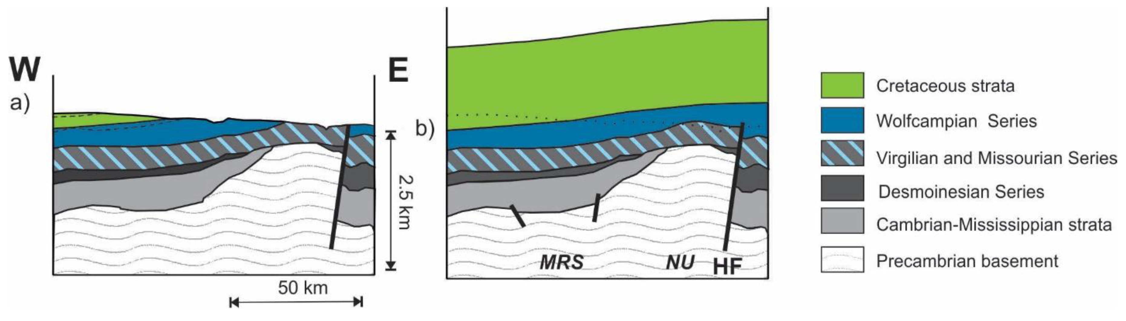
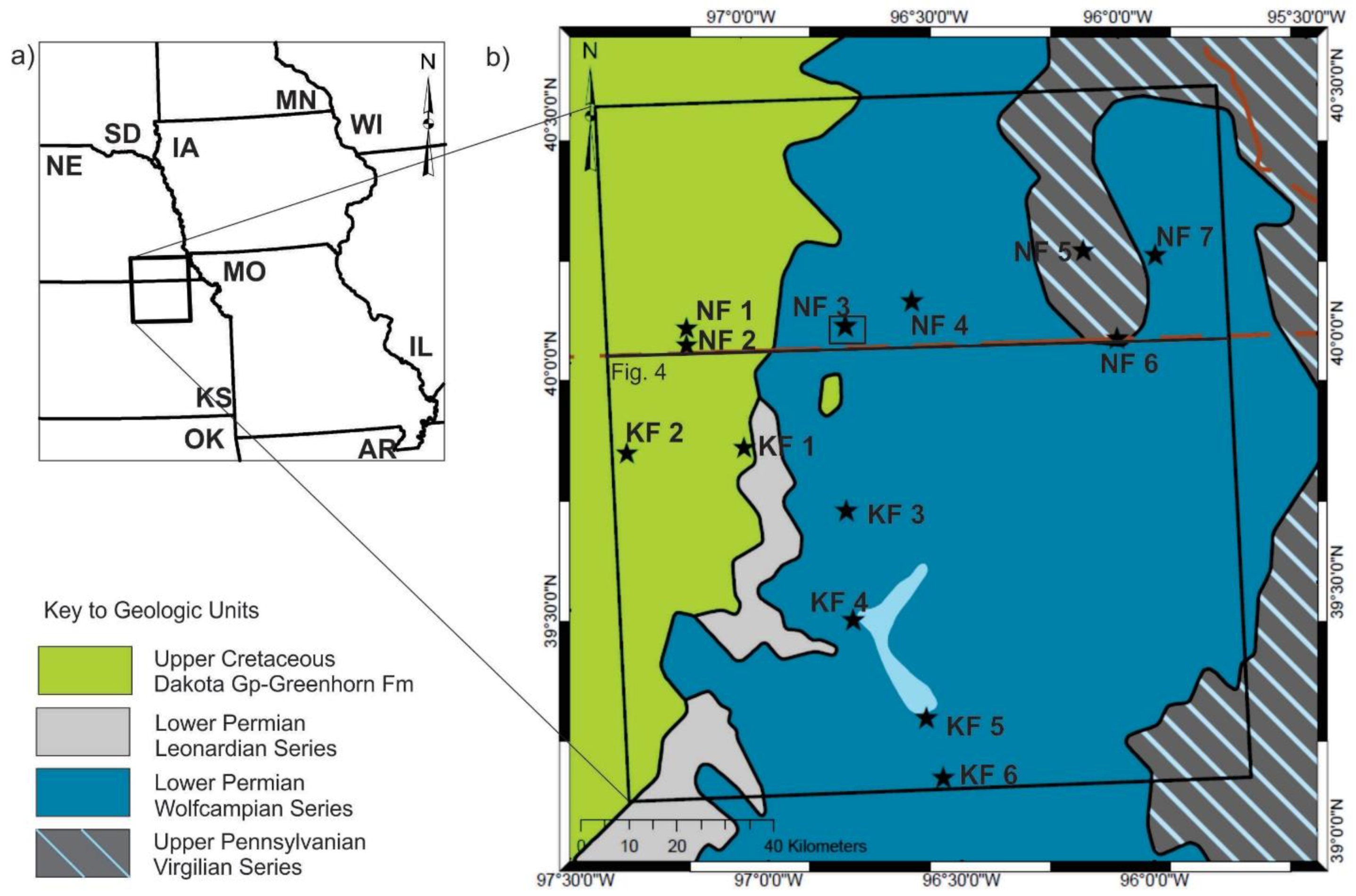
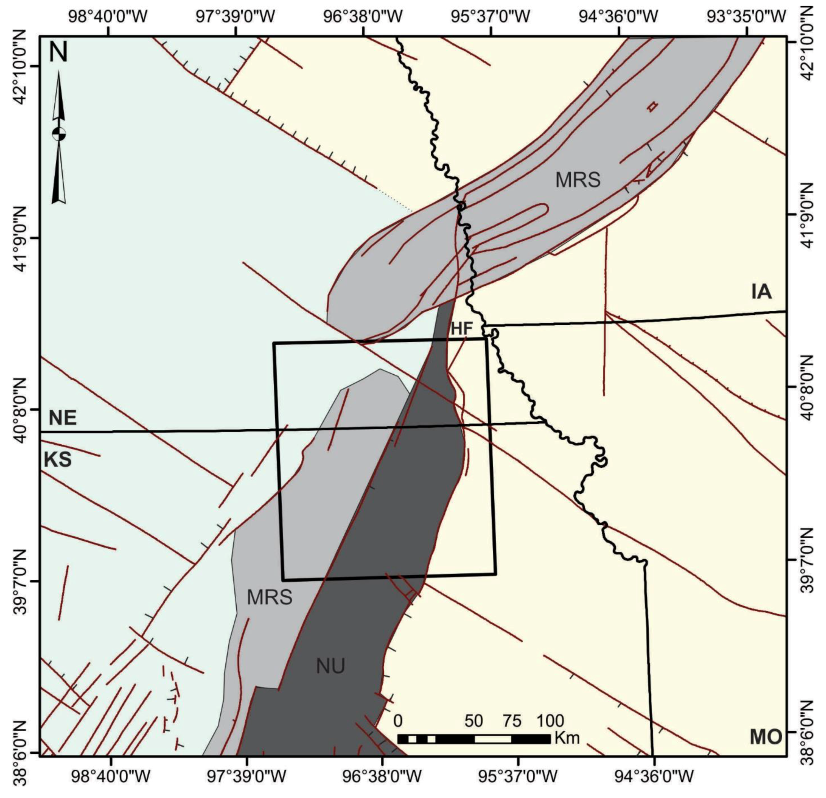
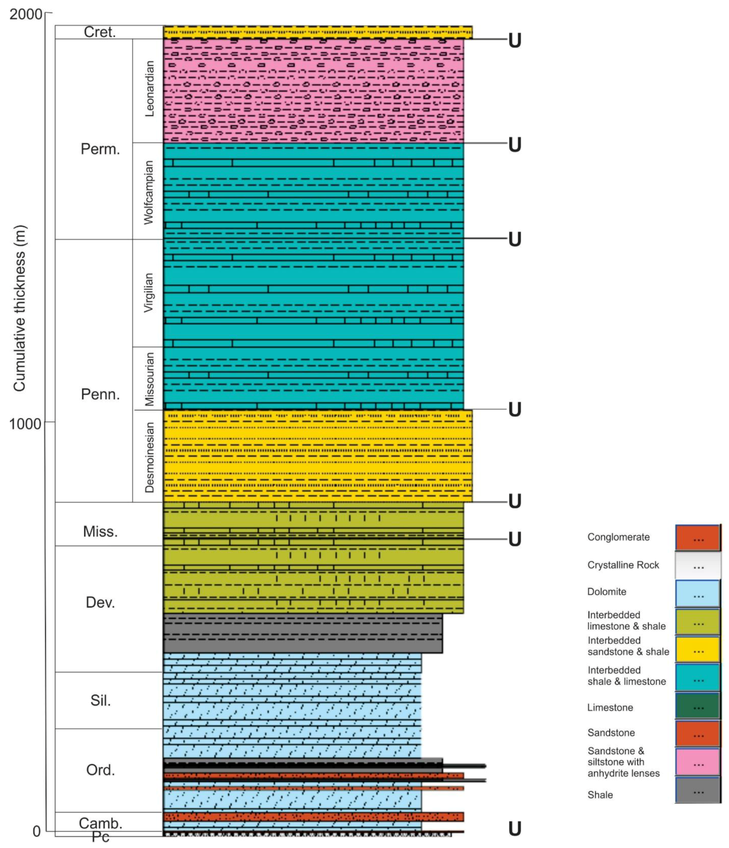
2. Geologic Setting
3. Methods
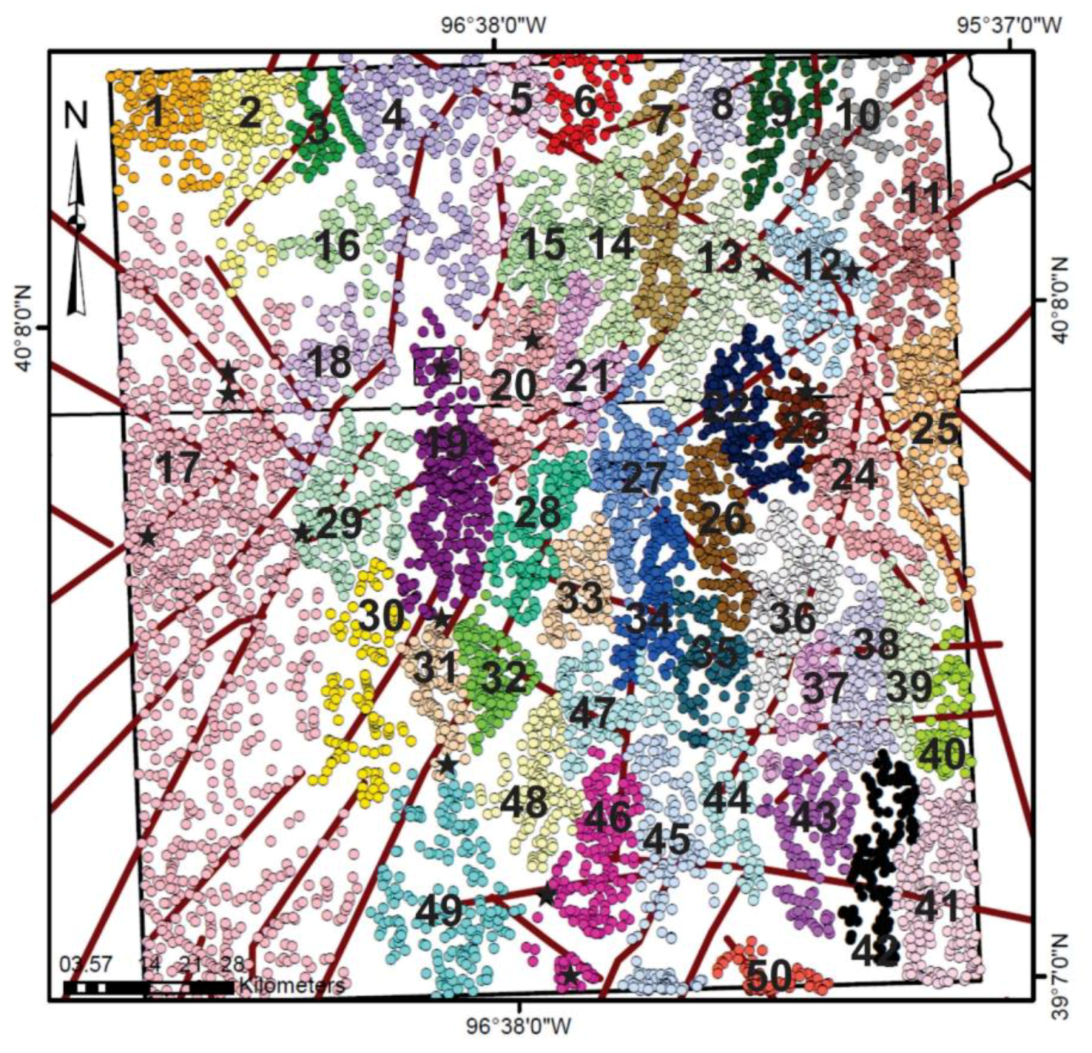
4. Results: Surface Lineament/Joint Data
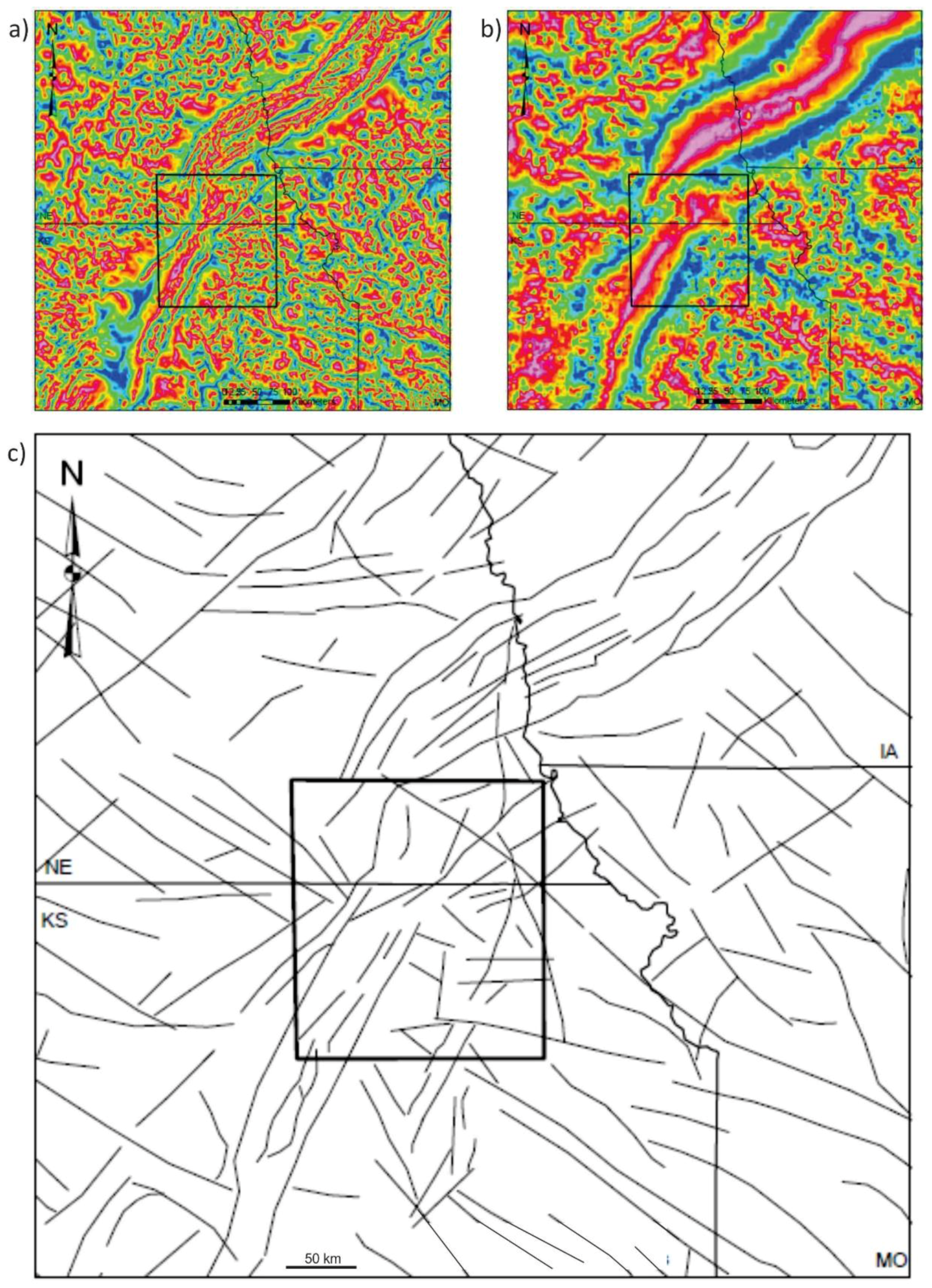
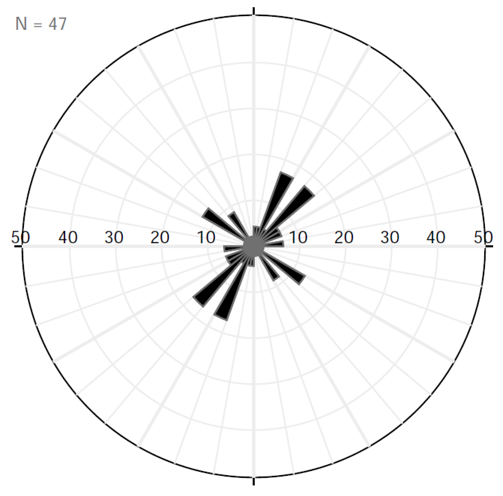
5. Results: Basement Lineaments from Potential Fields Data
6. Comparison and Interpretation of Surface and Basement Datasets
7. Discussion
8. Conclusions
Author Contributions
Acknowledgments
Conflicts of Interest
References
- Berberian, M. Master “blind” thrust faults hidden under the Zagros folds: Active basement tectonics and surface morphotectonics. Tectonophysics 1995, 241, 193–224. [Google Scholar] [CrossRef]
- Cinque, A.; Patacca, E.; Scandone, P.; Tozzi, M. Quaternary kinematic evolution of the Southern Appennines. Relationships between surface geological features and deep lithospheric structures. Ann. Geophys. 1993, 36, 249–260. [Google Scholar]
- Shephard-Thorn, E.R.; Lake, R.D.; Atitullah, M.E.; Gray, D.A. Basement control of structures in the Mesozoic rocks in the Strait of Dover region, and its reflexion in certain features of the present land and submarine topography. Phil. Trans. R. Soc. Lond. A 1972, 272, 99–110. [Google Scholar] [CrossRef]
- Butler, R.W.H.; Holdsworth, R.E.; Lloyd, G.E. The role of basement reactivation in continental deformation. J. Geol. Soc. 1997, 154, 69–71. [Google Scholar] [CrossRef]
- Thomas, W.A. Genetic relationship of rift-stage crustal structure, terrane accretion, and foreland tectonics along the southern Appalachian-Ouachita orogen. J. Geodyn. 2004, 37, 549–563. [Google Scholar] [CrossRef]
- Audet, P.; Burgmann, R. Dominant role of tectonic inheritance in supercontinent cycles. Nat. Geosci. 2011, 4, 184–187. [Google Scholar] [CrossRef]
- Huerta, A.D.; Harry, D.L. Wilson cycles, tectonic inheritance, and rifting of the North American Gulf of Mexico continental margin. Geosphere 2012, 8, 374–385. [Google Scholar] [CrossRef]
- Macedo, J.; Marshak, S. Controls on the geometry of fold-thrust belt salients. GSA Bull. 1999, 111, 1808–1822. [Google Scholar] [CrossRef]
- Gates, A.E.; Costa, R.E. Multiple Reactivation of Rigid Basement block margins, examples in the northern Reading Prong, USA. In Basement Tectonics 12; Proceedings of the International Conferences on Basement Tectonics; Hogan, J.P., Gilbert, M.C., Eds.; Springer: Dordrecht, The Netherlands, 1998; pp. 123–153. [Google Scholar]
- Molliex, S.; Bellier, O.; Terrier, M.; Lamarche, J.; Martelet, G.; Espurta, N. Tectonic and sedimentary inheritance on the structural framework of Provence (SE France): Importance of the Salon-Cavaillon fault. Tectonophysics 2010, 501, 1–16. [Google Scholar] [CrossRef] [Green Version]
- Said, A.; Baby, P.; Chardon, D.; Ouali, J. Structure, paleogeographic inheritance, and deformation history of the southern Atlas foreland fold and thrust belt of Tunisia. Tectonics 2011, 30. [Google Scholar] [CrossRef] [Green Version]
- McMechan, M.E. Deep transverse basement structural control of mineral systems in the southeastern Canadian Cordillera. Can. J. Earth Sci. 2012, 49, 693–708. [Google Scholar] [CrossRef]
- Burberry, C.M. The effect of basement fault reactivation on the Triassic-Recent geology of Kurdistan, N Iraq. J. Pet. Geol. 2015, 38, 37–58. [Google Scholar] [CrossRef]
- Sibson, R.H. A note on fault reactivation. J. Struct. Geol. 1985, 7, 751–754. [Google Scholar] [CrossRef]
- Letouzey, J. Fault reactivation, inversion and fold-thrust belt. In Proceedings of the 4th IFP Exploration and Production Research Conference, Bordeaux, France, 14–18 November 1988. [Google Scholar]
- Morris, A.; Ferrill, D.A.; Henderson, D.B. Slip-tendency analysis and fault reactivation. Geology 1996, 24, 275–278. [Google Scholar] [CrossRef]
- Dewey, J.F. Kinematics and Dynamics of Basin Inversion; Cooper, M.A., Williams, W.D., Eds.; Geological Society of London Special Publication: London, UK, 1989; Volume 44, p. 352. [Google Scholar]
- Williams, G.D.; Powell, C.M.; Cooper, M.A. Geometry and kinematics of inversion tectonics. In Inversion Tectonics; Cooper, M.A., Williams, G.D., Eds.; Geological Society of London Special Publication: London, UK, 1989; Volume 44, pp. 3–15. [Google Scholar]
- Ranalli, G. Rheology of the crust and its role in tectonic reactivation. J. Geodyn. 2000, 30, 3–15. [Google Scholar] [CrossRef]
- Del Ventisette, C.; Montanari, D.; Sani, F.; Bonini, M. Basin inversion and fault reactivation in laboratory experiments. J. Struct. Geol. 2006, 28, 2067–2083. [Google Scholar] [CrossRef]
- Handin, J. On the Coulomb-Mohr Failure Criterion. J. Geophys. Res. 1969, 74, 5343–5348. [Google Scholar] [CrossRef]
- Butler, R.W.H.; Tavarnelli, E.; Grasso, M. Structural inheritance in mountain belts: An Alpine Apennine perspective. J. Struct. Geol. 2006, 28, 1893–1908. [Google Scholar] [CrossRef]
- Dubois, A.; Odonne, F.; Massonnat, G.; Lebourg, T.; Fabre, R. Analogue modelling of fault reactivation: Tectonic inversion and oblique remobilisation of grabens. J. Struct. Geol. 2002, 24, 1741–1752. [Google Scholar] [CrossRef]
- Bahroudi, A.; Koyi, H.A. Effect of spatial distribution of Hormuz salt on deformation style in the Zagros fold and thrust belt: An analogue modelling approach. J. Geol. Soc. 2003, 160, 719–733. [Google Scholar] [CrossRef]
- Viola, G.; Odonne, F.; Mancktelow, N. Analogue modelling of reverse fault reactivation in strike–slip and transpressive regimes: Application to the Giudicarie fault system, Italian Eastern Alps. J. Struct. Geol. 2004, 26, 401–418. [Google Scholar] [CrossRef]
- Lisle, R.J.; Srivastava, D.C. Test of the frictional reactivation theory for faults and validity of fault-slip analysis. Geology 2004, 32, 569–572. [Google Scholar] [CrossRef]
- Burberry, C.M.; Joeckel, R.M.; Korus, J.T. Post-Mississippian Tectonic Evolution of the Nemaha Tectonic Zone and Midcontinent Rift System, SE Nebraska and N Kansas. Available online: https://digitalcommons.unl.edu/cgi/viewcontent.cgi?article=1471&context=geosciencefacpub (accessed on 10 April 2018).
- Neff, A.W. A Study of the Fracture Patterns of Riley County, Kansas. Master’s Thesis, Kansas State College of Agriculture and Applied Science, Manhattan, KS, USA, 1949. [Google Scholar]
- Ward, J.R. A Study of the Joint Patterns in Gently Dipping Sedimentary Rocks of South-Central Kansas; Kansas Geological Survey Bulletin: Lawrence, KS, USA, 1986. [Google Scholar]
- Baehr, W.M. An Investigation of the Relationship between Rock Structure and Drainage in the Southern Half of the Junction City, Kansas, Quadrangle. Master’s Thesis, Kansas State College of Agriculture and Applied Science, New York, NY, USA, 1954. [Google Scholar]
- Smith, J.W.; Kuntz, C.S.; Williams, A.L.; Scheper, R.J. Structural and Photographic Lineaments, Gravity, Magnetics and Seismicity of Central USA. In Proceedings of the First International Conference on the New Basement Tectonics, Salt Lake City, UT, USA, 3–7 June 1974; pp. 163–168. [Google Scholar]
- White, D.C. Lineament Study of Stream Patterns in a Portion of East-Central Kansas. Master’s Thesis, Emporia State University, Emporia, KS, USA, 1990. [Google Scholar]
- Nelson, P.D. The Reflection of the Basement Complex in the Surface Structures of the Marshall-Riley County area of Kansas. Master’s Thesis, Kansas State College of Agriculture and Applied Science, Manhattan, KS, USA, 1952. [Google Scholar]
- Garrity, C.P.; Soller, D.R. Database of the Geologic Map of North America; Adapted from the Map by J.C. Reed, Jr. and Others (2005): U.S. Geological Survey Data Series 424. 2009. Available online: https://pubs.usgs.gov/ds/424/ (accessed on 10 April 2018).
- Carlson, M. Tectonic implications and influence of the midcontinent rift system in Nebraska and adjoining areas. In Basement Tectonics 10, Proceedings of the International Conferences on Basement Tectonics; Ojakangas, R.W., Dickas, A.B., Green, J.C., Eds.; Springer: Dordrecht, The Netherlands, 1995; Volume 4, pp. 61–64. [Google Scholar]
- Jewett, J.M.; Merriam, D.F. Geologic framework of Kansas; a review for geophysicists. Bull.-Kansas Geol. Surv. 1959, 137, 9–52. [Google Scholar]
- Anderson, K.H.; Wells, J.S. Forest City Basin of Missouri, Kansas Nebraska and Iowa. AAPG Bull. 1968, 52, 264–281. [Google Scholar] [CrossRef]
- Condra, G.E.; Reed, E.C. The Geological Section of Nebraska. Neb. Geol. Surv. Bull. 1959, 14A, 82. Available online: http://www.nogcc.ne.gov/ResearchDocuments/Number14.pdf (accessed on 10 April 2018).
- Baars, D.L. Conjugate basement rift zones in Kansas, Midcontinent, USA. In Basement Tectonics 9, Proceedings of the International Conferences on Basement Tectonics, Canberra, Australia, 2–6 July 1990; Rickard, M.J., Harrington, H.J., Williams, P.R., Eds.; Springer: Dordrecht, The Netherlands, 1992; Volume 3, pp. 201–210. [Google Scholar]
- Carlson, M.P.; Treves, S. The Elk Creek carbonatite, southeast Nebraska—An overview. Nat. Resour. Res. 2005, 14, 39–45. [Google Scholar] [CrossRef]
- Carlson, M.P. Tectonic Implications and Influence of the Midcontinent Rift System in Nebraska and Adjoining Areas; GSA Special Paper: Washington, DC, USA, 1997; Volume 312, pp. 231–234. [Google Scholar]
- Berendsen, P. Tectonic Evolution of the Midcontinent Rift System in Kansas; GSA Special Paper; Geological Society of America: Boulder, CO, USA, 1997; Volume 312, pp. 235–241. [Google Scholar]
- Atekwana, E. Precambrian Basement Beneath the Central Midcontinent United States as Interpreted from Potential Field Imagery; GSA Special Paper; Geological Society of America: Boulder, CO, USA, 1996; Volume 308, pp. 33–44. [Google Scholar]
- Carlson, M.P. Precambrian accretionary history and Phanerozoic structures—A unified explanation for the tectonic architecture of the Nebraska region, USA. GSA Mem. 2007, 200, 321–326. [Google Scholar]
- Whitmeyer, S.J.; Karlstrom, K.E. Tectonic model for the Proterozoic growth of North America. Geosphere 2007, 3, 220–259. [Google Scholar] [CrossRef]
- Carlson, M.P.; Treves, S.B.; Goble, R.J.; Xu, A. New Data and Interpretations for the Precambrian, Midcontinent USA. In Basement Tectonics; Springer: Dordrecht, The Netherlands, 1999; pp. 49–63. [Google Scholar]
- Carlson, M. Evidence from the stratigraphic record for basement deformation in southeastern Nebraska, Midcontinent USA. In Basement Tectonics 12, Central North America and Other Regions, Proceedings of the International Conferences on Basement Tectonics, Norman, Oklahoma, 21–26 May 1995; Hogan, J.P., Gilbert, M.C., Eds.; Springer: Dordrecht, The Netherlands, 1998; Volume 6, p. 227. [Google Scholar]
- Scotese, C.R.; Golonka, J. PALEOMAP Paleogeographic Atlas: Arlington; Department of Geology, University of Texas: Austin, TX, USA, 1992. [Google Scholar]
- Goebel, E.D. Mississippian rocks of western Kansas. AAPG Bull. 1968, 52, 1732–1778. [Google Scholar]
- Craddock, J.P.; Pearson, A.; McGovern, M.; Kropf, E.; Moshoian, A.; Donnelly, K. Post-Extension Shortening Strains Preserved in Calcites of the Midcontinent Rift; GSA Special paper: Washington, DC, USA, 1997; Volume 312, pp. 115–126. [Google Scholar]
- Hauser, E.C. Midcontinent Rifting in a Grenville Embrace; GSA Special Publication: Washington, DC, USA, 1996; Volume 308, pp. 67–75. [Google Scholar]
- Eardley, A.J. Structural Geology of North America; Harper Row: New York, NY, USA, 1962; 743p. [Google Scholar]
- Berendsen, P.; Speczik, S. Sedimentary environment of Middle Ordovician iron oolites in northeastern Kansas, USA. Acta Geol. Pol. 1991, 41, 215–226. [Google Scholar]
- Berendsen, P.; Doveton, J.H.; Speczik, S. Distribution and characteristics of a Middle Ordovician oolitic ironstone in northeastern Kansas based on petrographic and petrophysical properties: A Laurasian ironstone case study. Sediment. Geol. 1992, 76, 207–219. [Google Scholar] [CrossRef]
- Mendenhall, R.A. Surface Geology of Bala, Riley County, Kansas. Master’s Thesis, Kansas State College of Agriculture and Applied Science, Manhattan, KS, USA, 1958. [Google Scholar]
- Wilson, F.W.; Berendsen, P. The role of recurrent tectonics in the formation of the Nemaha uplift and Cherokee-forest city basins and adjacent structures in eastern Kansas and contiguous states, USA. In Basement Tectonics 12, Central North America and Other Regions, Proceedings of the International Conferences on Basement Tectonics, Norman, Oklahoma, 21–26 May 1995; Hogan, J.P., Gilbert, M.C., Eds.; Springer: Dordrecht, The Netherlands, 1998; Volume 6, pp. 301–302. [Google Scholar]
- Brown, L.; Serpa, L.; Setzer, T.; Oliver, J.; Kaufman, S.; Lillie, R.; Steiner, D.; Steeples, D.W. Intracrustal complexity in the United States midcontinent: Preliminary results from COCORP surveys in northeastern Kansas. Geology 1983, 11, 25–30. [Google Scholar] [CrossRef]
- Serpa, L.; Setzer, T.; Brown, L. COCORP Seismic-Reflection Profiling in Northeastern Kansas, In Geophysics in Kansas; Steeples, D.W., Ed.; Kansas Geological Survey: Lawrence, KS, USA, 1989; Volume 226, pp. 165–176. [Google Scholar]
- Gay, S.P., Jr. Strike-slip compressional thrust-fold nature of the Nemaha System in Eastern Kansas and Oklahoma. In Proceedings of the Transactions of the 1999 AAPG Midcontinent Section Meeting, Wichita, KS, USA, 29–31 August 1999; pp. 39–50. [Google Scholar]
- Moore, R.C. Early Pennsylvanian deposits west of the Nemaha Granite Ridge, Kansas. AAPG Bull. 1926, 10, 205–216. [Google Scholar]
- Heckel, P.H. Pennsylvanian cyclothems in Midcontinent North America as far-field effects of waxing and waning of Gondwana ice sheets. In Resolving the Late Paleozoic Ice Age in Time and Space; Fielding, C.R., Frank, T.D., Isbell, J.L., Eds.; Geological Society of America: Boulder, CO, USA, 2008. [Google Scholar]
- Heckel, P.H. Pennsylvanian stratigraphy of Northern Midcontinent Shelf and biostratigraphic correlation of cyclothems. Stratigraphy 2013, 10, 3–39. [Google Scholar]
- Moore, R.C. Paleoecological aspects of Kansas Pennsylvanian and Permian cyclothems. In Symposium on Cyclic Sedimentation; Kansas Geological Survey Bulletin: Lawrence, KS, USA, 1964; pp. 287–380. [Google Scholar]
- West, R.R.; Miller, K.B.; Watney, W.L. The Permian System in Kansas; Kansas Geological Survey Bulletin: Lawrence, KS, USA, 2010. [Google Scholar]
- Kluth, C.F.; Koney, P.J. Plate tectonics of the Ancestral Rocky Mountains. Geology 1981, 9, 10–15. [Google Scholar] [CrossRef]
- Joeckel, R.M.; Nicklen, B.L.; Carlson, M.P. Low-accommodation detrital apron alongside a basement uplift, Pennsylvanian of Midcontinent North America. Sediment. Geol. 2007, 197, 165–187. [Google Scholar] [CrossRef]
- Leary, R.J.; Umhoefer, P.; Smith, M.E.; Riggs, N. A three-sided orogen: A new tectonic model for Ancestral Rocky Mountain uplift and basin development. Geology 2017, 45, 735–738. [Google Scholar] [CrossRef]
- Merriam, D.F.; Forster, A. Stratigraphic and Sedimentological Evidence for Late Paleozoic Earthquakes and Recurrent Structural Movement in the US Midcontinent; Geological Society of America: Boulder, CA, USA, 2002. [Google Scholar]
- Underwood, J.R.; Polson, A. Spillway Fault System, Tuttle Creek Reservoir, Pottawatomie County, Northeastern Kansas; Geological Society of America: Boulder, CA, USA, 1988. [Google Scholar]
- Yonkee, W.A.; Weil, A.B. Tectonic evolution of the Sevier and Laramide belts within the North American Cordillera orogenic system. Earth-Sci. Rev 2015, 150, 531–593. [Google Scholar] [CrossRef] [Green Version]
- Tikoff, B.; Maxson, J. Lithopsheric buckling of the Laramide Foreland during Late Cretaceous and Paleogene, Western United States. Rocky Mt. Geol. 2001, 36, 13–35. [Google Scholar] [CrossRef]
- Ohlmacher, G.C.; Berendsen, P. Kinematics, mechanics, and potential earthquake hazards for faults in Pottawatomie County, Kansas. USA. Tectonophysics 2005, 396, 227–244. [Google Scholar] [CrossRef]
- Steeples, D.W.; DuBois, S.M.; Wilson, F.W. Seismicity, faulting, and geophysical anomalies in Nemaha County, Kansas: Relationship to regional structures. Geology 1979, 7, 134–138. [Google Scholar] [CrossRef]
- Burchett, R.R. Earthquakes in Nebraska: Educational Circular; Conservation and Survey Division, University of Nebraska: Lincoln, NE, USA, 1990. [Google Scholar]
- Tucker, C.J.; Grant, D.M.; Dykstra, J.D. NASA’s global orthorectified Landsat data set. Photogramm. Eng. Remote Sens. 2004, 70, 313–322. [Google Scholar] [CrossRef]
- Bankey, V.; Cuevas, A.; Daniels, D.; Finn, C.A.; Hernandez, I.; Hill, P.; Kucks, R.; Miles, W.; Pilkington, M.; Roberts, C.; et al. Digital Data Grids for the Magnetic Anomaly Map of North America: U.S. Geological Survey Open-File Report 02-414; U.S. Geological Survey: Denver, CO, USA, 2002. Available online: https://mrdata.usgs.gov/magnetic/ (accessed on 10 April 2018).
- Kucks, R.P. Bouguer Gravity Anomaly Data Grid for the Conterminous US; U.S. Geological Survey: Denver, CO, USA, 1999. Available online: https://mrdata.usgs.gov/gravity/ (accessed on 10 April 2018).
- Verduzco, B.; Fairhead, J.D.; Green, C.M.; MacKenzie, C. New insights into magnetic derivatives for structural mapping. Lead. Edge 2004, 23, 116–119. [Google Scholar] [CrossRef]
- Ladeira, F.L.; Price, N.J. Relationship between fracture spacing and bed thickness. J. Struct. Geol. 1981, 3, 179–183. [Google Scholar] [CrossRef]
- Stearns, D.W. Faulting and forced folding in the Rocky Mountains foreland. In Laramide Folding Associated with Basement Block Faulting in the Western United States; Memoir; Geological Society of America: Boulder, CO, USA, 1978; Volume 151, pp. 1–37. [Google Scholar]
- Cosgrove, J.W.; Ameen, M.S. A comparison of the geometry, spatial organization and fracture patterns associated with forced folds and buckle folds. In Forced Folds and Fractures; Cosgrove, J.W., Ameen, M.S., Eds.; Geological Society Special Publication: London, UK, 2000; pp. 7–21. [Google Scholar]
- Luneburg, C.; Ratliff, B.; Page, A. Structural Analysis for Fracture Optimization; AAPG Search and Discovery Article: Tulsa, OK, USA, 2015. [Google Scholar]
- Gutierrez, I. Application of Trishear and Elastic Dislocation Models to the Teapot Anticline, Wyoming. Master’s Thesis, University of Stavanger, Stavanger, Norway, 2017. [Google Scholar]
- Erslev, E.A. Trishear fault-propagation folding. Geology 1991, 19, 617–620. [Google Scholar] [CrossRef]
- Bellahsen, N.; Fiore, P.; Pollard, D.D. The role of fractures in the structural interpretation of Sheep Mountain Anticline, Wyoming. J. Struct. Geol. 2006, 28, 850–867. [Google Scholar] [CrossRef]
- Erslev, E.A.; Koenig, N.V. Three-dimensional kinematics of Laramide, basement-involved Rocky Mountain deformation, USA: Insights from minor faults and GIS-enhanced structure maps. Geol. Soc. Am. Mem. 2009, 204, 125–150. [Google Scholar] [CrossRef]
- Fischer, M.P.; Wilkerson, M.S. Predicting the orientation of joints from fold shape: Results of pseudo–three-dimensional modeling and curvature analysis. Geology 2000, 28, 15–18. [Google Scholar] [CrossRef]
- Ahmadhadi, F.; Lacombe, O.; Daniel, J.M. Early reactivation of basement faults in Central Zagros (SW Iran): Evidence from pre-folding fracture populations in Asmari Formation and lower Tertiary paleogeography. In Thrust Belts and Foreland Basins; Springer: Berlin/Heidelberg, Germany, 2007; pp. 205–228. [Google Scholar]
- Wicks, J.L.; Dean, S.L.; Kulander, B.R. Regional tectonics and fracture patterns in the Fall River Formation (Lower Cretaceous) around the Black Hills foreland uplift, western South Dakota and northeastern Wyoming. In Forced Folds and Fractures; Cosgrove, J.W., Ameen, M.S., Eds.; Geological Society Special Publication: London, UK, 2000; pp. 145–165. [Google Scholar]
- Engelder, T. Joints and shear fractures in rock. In Fracture Mechanics of Rock; Atkinson, B.K., Ed.; Academic Press Inc.: London, UK, 1987; pp. 27–69. [Google Scholar]
- Pollard, D.D.; Aydin, A. Progress in Understanding Jointing Over the Past Century. Geol. Soc. Am. Bull. 1988, 100, 1181–1204. [Google Scholar] [CrossRef]
- Davis, G.H.; Reynolds, S.J.; Kluth, C. Structural Geology of Rocks and Regions, 3rd ed.; John Wiley and Sons, Inc.: New York, NY, USA, 2012; 884p. [Google Scholar]
- Odling, N.E.; Gillespie, P.; Bourgine, B.; Castaing, C.; Chiles, J.P.; Christensen, N.P.; Fillion, E.; Genter, A.; Olsen, C.; Thrane, L.; et al. Variations in fracture system geometry and their implications for fluid flow in fractures hydrocarbon reservoirs. Pet. Geosci. 1999, 5, 373–384. [Google Scholar] [CrossRef]
- Burberry, C.M.; Peppers, M.H. Fracture Characterization in Tight Carbonates: An example from the Ozark Plateau, AR. AAPG Bull. 2017, 101, 1675–1696. [Google Scholar] [CrossRef]
- Burberry, C.M.; Cannon, D.L.; Cosgrove, J.W.; Engelder, T. Fracture patterns associated with the evolution of the Teton anticline, Sawtooth Range, Montana. Rev. Geol. Soc. Lond. Spec. Publ. 2018. [Google Scholar] [CrossRef]
- McQuillan, H. Fracture Patterns on Kuh-e Asmari Anticline, SW Iran. AAPG Bull. 1974, 58, 236–245. [Google Scholar]
- Siddoway, C. Potential Sources of Crustal Anistotropy in the Wyoming Province: Insights from Basement Structures of the Bighorn Mountains, Wyoming; Geological Society of America Abstracts with Programs; Geological Society of America: Boulder, CO, USA, 2011; Volume 42, p. 435. [Google Scholar]


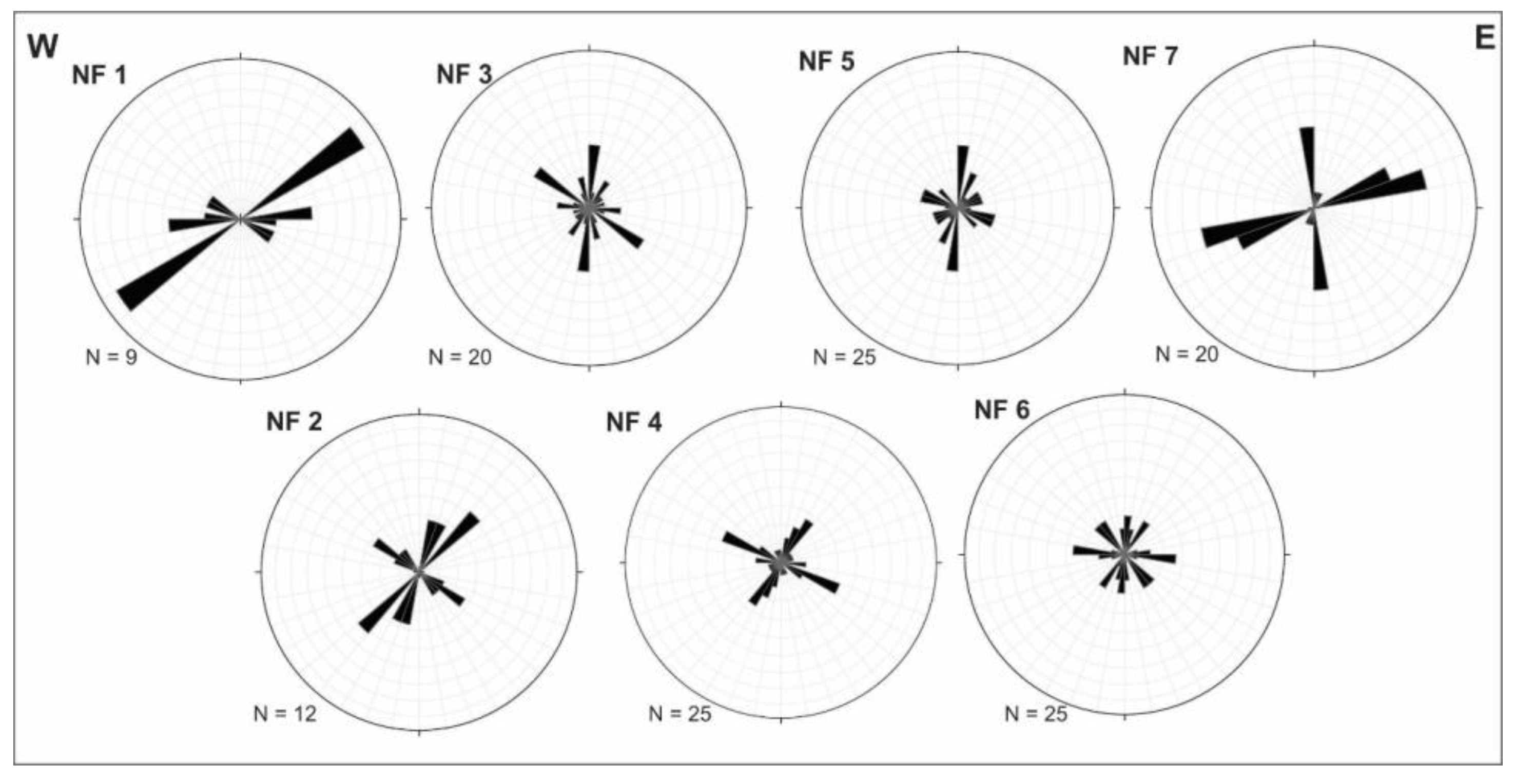
| Location | Prominent Joint Orientations Based on Rose Diagram Bins | |||||||||||
|---|---|---|---|---|---|---|---|---|---|---|---|---|
| NF 1 | 057 | 088 | 110 | |||||||||
| NF 2 | 016 | 040 | 053 | 125 | ||||||||
| NF 3 | 002 | 031 | 047 | 090 | 122 | |||||||
| NF 4 | 029 | 072 | 117 | |||||||||
| NF 5 | 004 | 026 | 049 | 068 | 096 | 115 | ||||||
| NF 6 | 353 | 034 | 090 | 105 | 135 | |||||||
| NF 7 | 353 | 019 | 062 | 073 | ||||||||
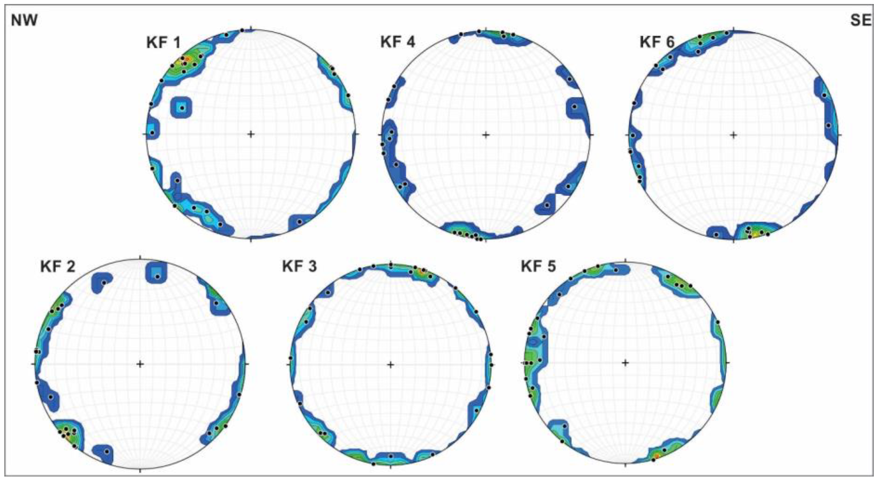
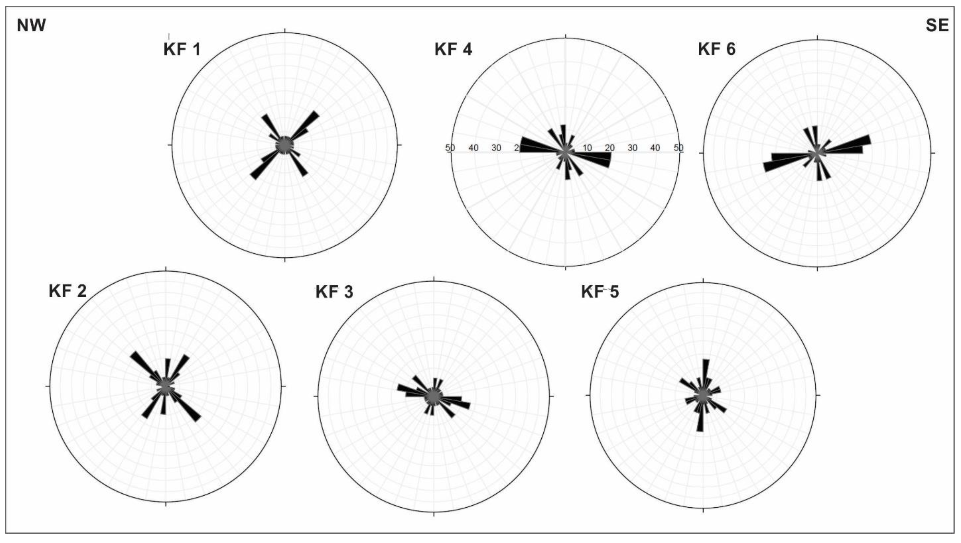
| KF 1 | 003 | 022 | 060 | 084 | 117 | 139 | ||||||
| KF 2 | 008 | 037 | 111 | 136 | 165 | |||||||
| KF 3 | 359 | 029 | 068 | 090 | 110 | 137 | ||||||
| KF 4 | 357 | 029 | 049 | 072 | 106 | 148 | ||||||
| KF 5 | 003 | 021 | 060 | 072 | 137 | 162 | ||||||
| KF 6 | 359 | 020 | 045 | 078 | 100 | 161 | ||||||
| Representative | 001 | 020 | 031 | 046 | 059 | 072 | 090 | 110 | 124 | 137 | 148 | 163 |
| ETM | 005 | 055 | 085 | 115 | 145 | |||||||
| Age of Host Fm | Prominent Joint Orientations Based on Rose Diagram Bins | |||||||||||
|---|---|---|---|---|---|---|---|---|---|---|---|---|
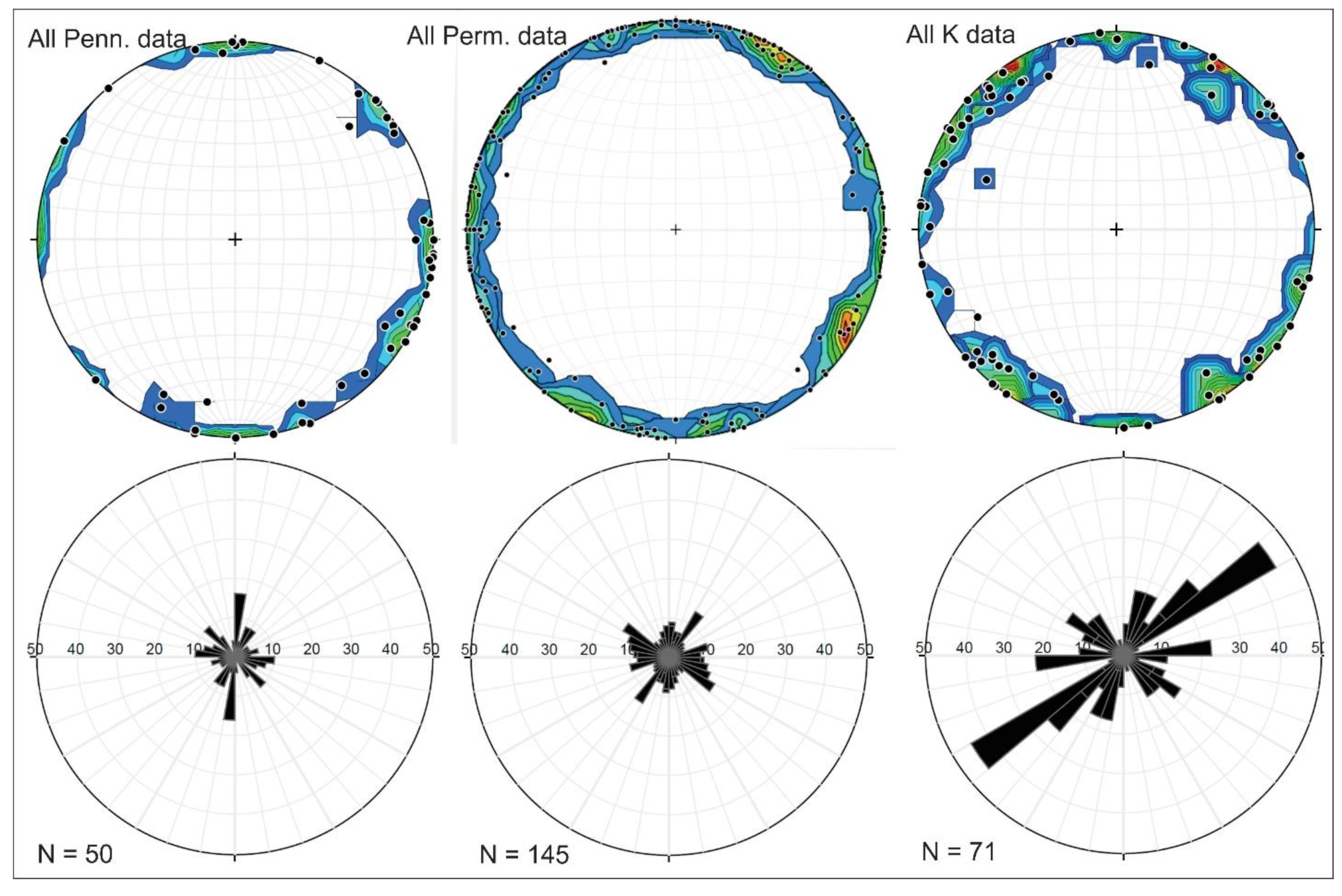
| All Penn | 003 | 028 | 069 | 091 | 113 | 135 | ||||||
| All Perm | 003 | 029 | 074 | 098 | 118 | 159 | ||||||
| All K | 004 | 015 | 040 | 050 | 089 | 110 | 122 | 161 | ||||
| Representative (Table 1) | 001 | 020 | 031 | 046 | 059 | 072 | 090 | 110 | 124 | 137 | 148 | 163 |
| ETM | 005 | 055 | 085 | 115 | 145 | |||||||
| Dataset | Prominent Joint Orientations (Peaks on Rose Diagrams) | |||||||||||
|---|---|---|---|---|---|---|---|---|---|---|---|---|
| Potential Fields | 025 | 045 | 125 | 135 | ||||||||
| Representative (Table 1) | 001 | 020 | 031 | 046 | 059 | 072 | 090 | 110 | 124 | 137 | 148 | 163 |
| ETM | 005 | 055 | 085 | 115 | 145 | |||||||
© 2018 by the authors. Licensee MDPI, Basel, Switzerland. This article is an open access article distributed under the terms and conditions of the Creative Commons Attribution (CC BY) license (http://creativecommons.org/licenses/by/4.0/).
Share and Cite
Burberry, C.M.; Swiatlowski, J.L.; Searls, M.L.; Filina, I. Joint and Lineament Patterns across the Midcontinent Indicate Repeated Reactivation of Basement-Involved Faults. Geosciences 2018, 8, 215. https://doi.org/10.3390/geosciences8060215
Burberry CM, Swiatlowski JL, Searls ML, Filina I. Joint and Lineament Patterns across the Midcontinent Indicate Repeated Reactivation of Basement-Involved Faults. Geosciences. 2018; 8(6):215. https://doi.org/10.3390/geosciences8060215
Chicago/Turabian StyleBurberry, Caroline M., Jerlyn L. Swiatlowski, Mindi L. Searls, and Irina Filina. 2018. "Joint and Lineament Patterns across the Midcontinent Indicate Repeated Reactivation of Basement-Involved Faults" Geosciences 8, no. 6: 215. https://doi.org/10.3390/geosciences8060215