A Numerical 1.5D Method for the Rapid Simulation of Geophysical Resistivity Measurements

Abstract

In some geological formations, borehole resistivity measurements can be simulated using a sequence of 1D models. By considering a 1D layered media, we can reduce the dimensionality of the problem from 3D to 1.5D via a Hankel transform. The resulting formulation is often solved via a semi-analytic method, mainly due to its high performance. However, semi-analytic methods have important limitations such as, for example, their inability to model piecewise linear variations on the resistivity. Herein, we develop a multi-scale finite element method (FEM) to solve the secondary field formulation. This numerical scheme overcomes the limitations of semi-analytic methods while still delivering high performance. We illustrate the performance of the method with numerical synthetic examples based on two symmetric logging-while-drilling (LWD) induction devices operating at 2 MHz and 500 KHz, respectively.

1. Introduction

There exist a wide variety of geophysical prospection methods. In this work, we focus on resistivity methods. We categorize these resistivity prospection methods according to their acquisition location as (a) on surface, such as the ones obtained using controlled sources electromagnetics (CSEM) [1,2,3] and magnetotelluric [4], and (b) in the borehole, such as the ones obtained using logging-while-drilling (LWD) devices. LWD is a technology that conveys borehole logging tools (e.g., gamma ray, resistivity, density, and sonic) downhole, record measurements, and transmit them to the subsurface for real time interpretation while the hole is being drilled [5,6,7,8,9,10,11,12]. These tools provide two pieces of information: (a) real-time data, which is processed on the field while drilling, and (b) data that is stored in the device to process after pulling it out from the hole. We use real-time data to evaluate the formation for geosteering, which is the act of adjusting inclination and azimuth angles of the borehole to reach a geological target [5,6,7,8,9,10,11].

The first commercial LWD device appeared in the 1970s. They were commercially used for formation evaluation, especially in high-angle wells. Nowadays, LWD devices are used both for reservoir characterization [6,7,8] and geosteering applications [9,10,11]. Modern borehole resistivity instruments can measure all nine couplings of the magnetic field, namely $xx$, $xy$, $xz$, $yx$, $yy$, $yz$, $zx$, $zy$ and $zz$ couplings (the first letter indicates the orientation of the transmitter and the second one indicates the receiver orientation) [13,14].

Since the depth of investigation of LWD resistivity measurements is limited compared to the assumed thickness of the geological layers, it is common to approximate subsurface models in the proximity of the logging instrument with a sequence of 1D models [5]. In a 1D model, we reduce the dimension of the problem via a Hankel or a 2D Fourier transform along the directions over which we assume the material properties to be invariant [15,16,17]. The resulting ordinary differential equations (ODEs) can be solved (a) analytically, leading to a semi-analytic approach after the numerical inversion of a Hankel transform [15,17,18,19,20], or (b) numerically, leading to a numerical approach [16].

Solving the ODEs analytically has some major limitations, for example, (a) the analytical solution can only account for piecewise constant material properties and other resistivity distributions cannot be solved analytically, which prevents to properly model, for example, an oil-to-water transitioning zone when fluids are considered to be immiscible; (b) a specific set of cumbersome formulas has to be derived for each physical process (e.g., electromagnetism, elasticity, etc.) anisotropy type, etc.; (c) analytical derivatives of certain models (e.g., cross-bedded formations, or derivatives with respect to the bed boundary positions) are often difficult to obtain and have not been published to the best of our knowledge [13].

Solving the resulting ODEs numerically is also possible. The resulting method also exhibits a linear cost with respect to the discretization size, since it consists of a sequence of independent 1D problems. An example of this approach can be found in [16], where Davydycheva et al. use a 2D Fourier transform to reduce the dimension of the problem. Then, they employ a highly accurate 1D finite difference method (FDM) to solve the resulting ODEs. This method is relatively simple to code. However, this combined methodology requires a computational cost that is over 1000 times larger than that observed in semi-analytical methods. This occurs due to the elevated number of unknowns required to properly discretize the ODEs. If a common factorization of the system matrix based on a lower and an upper triangular matrix (the so-called LU factorization) would be precomputed for all source positions, the situation would only worsen: one would need a refined grid to properly model all sources, and since the cost of backward substitution is also proportional to the discretization size (as it occurs with the LU factorization), the large computational cost required to perform backward substitution would significantly increase the total cost of the solver. The use of other traditional techniques such as a finite element method (FEM) (see, e.g., [21]) to solve the resulting ODEs would not alleviate those problems. Additionally, in [16], the use of a 2D Fourier transform presents another burden on the performance of the solver, since the number of ODEs (and the total solver cost) increases quadratically with respect to the number of integration points of the 1D Inverse Fourier Transform (IFT), while in the case of a Hankel Transform, the cost only grows linearly with respect to the number of integration points on the 1D Inverse Hankel Transform (IHT).

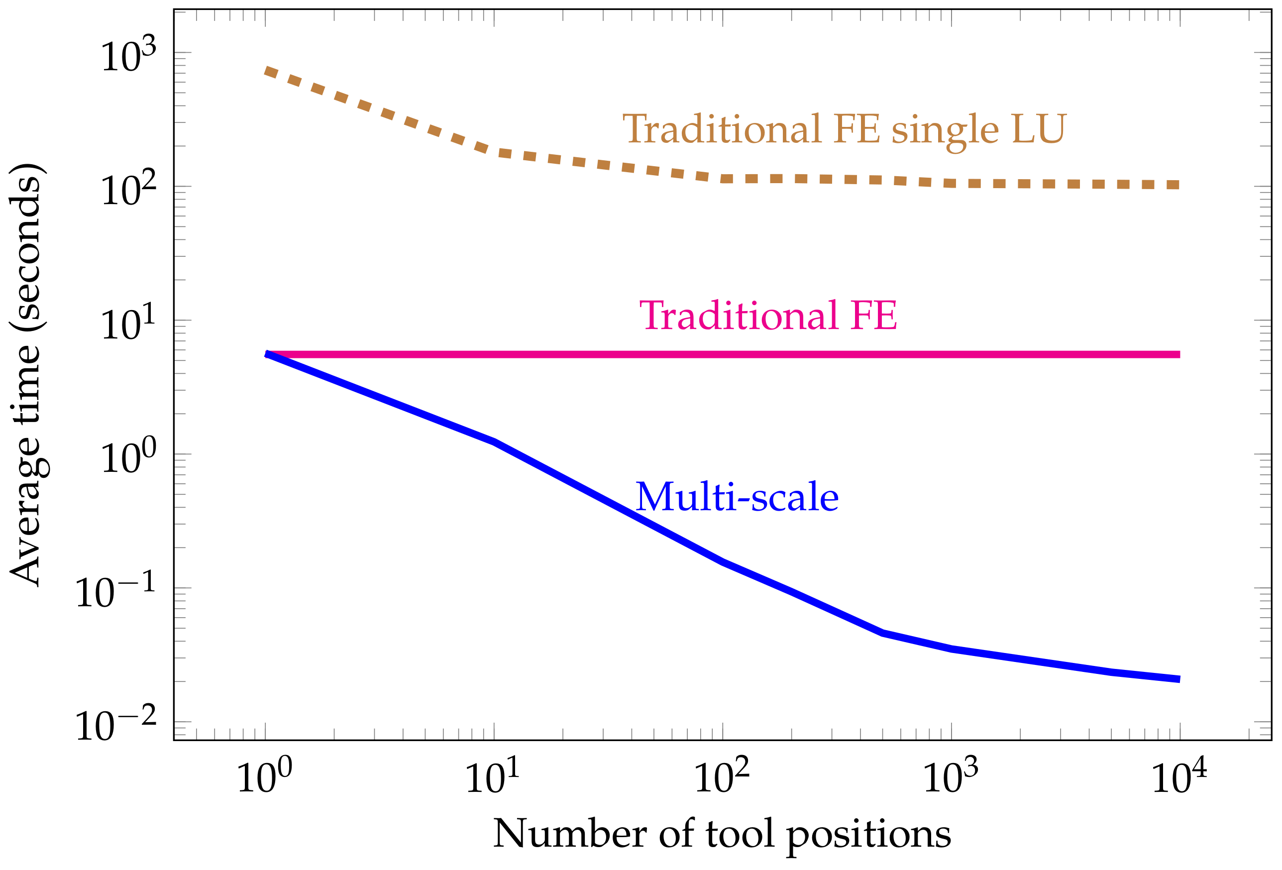
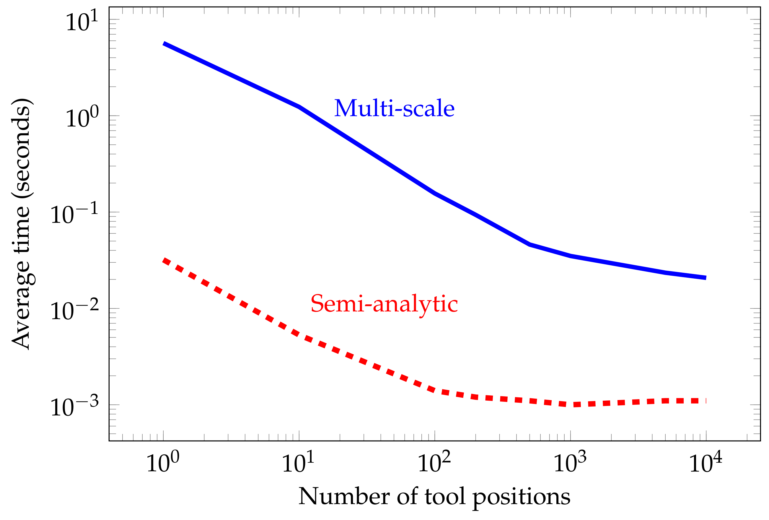
The main objective of this work is to overcome the above limitations of both semi-analytic and existing numerical methods by solving each 1D problem (associated with a Hankel mode) using an efficient multi-scale FEM. Additionally, we seek a method with the following features: (a) we can consider arbitrary resistivity distributions along the 1D direction, and (b) we can easily and rapidly construct derivatives with respect to the material properties and position of the bed boundaries by using an adjoint formulation, which allows us to compute numerically the derivatives forming the Jacobian matrix needed by the Gauss-Newton inversion method at (almost) no additional cost. Despite these advances, presently our proposed multi-scale method is slower than the semi-analytic one. However, it is approximately two orders of magnitude faster than a traditional 1D FEM or a 1D FDM, like the one presented in [16]. This speedup is essential for practical applications since one often needs to simulate thousands of logging positions and estimate millions of derivatives to solve a real-time inversion problems in the field for geosteering operations. Additionally, we employ a 1D Hankel transform rather than a 2D Fourier transform. This leads to a more complex mathematical formulation, but the resulting method exhibits a superior performance due to the lower number of ODEs that need to be solved.

In this work, we consider two traditional symmetric LWD tools available from oil service companies. Each of them contains two transmitters and two receivers. The receivers are symmetrically located at different sides of the transmitters [22].

2. 3D Formulation

In this section, we describe the strong and weak formulations for our three dimensional (3D) electromagnetic (EM) problem.

2.1. Strong Formulation

Let $\mathbf{\sigma }(x,y,z)$ be the real-valued conductivity tensor with positive determinant. Let $\mathbf{J}$ be a volumetric current source density and $\mathbf{M}$ a magnetic volumetric current source. Then, the EM fields satisfy Maxwell’s equations in 3D space [23]:

$$\begin{array}{cc}\hfill \nabla \times \mathcal{H}& =\left(\mathbf{\sigma }-i\omega \mathbf{\epsilon }\right)\mathcal{E}+\mathbf{J},\hfill \end{array}$$

(1)

$$\begin{array}{cc}\hfill \nabla \times \mathcal{E}& =i\omega \mathbf{\mu }\mathcal{H}+i\omega \mathbf{\mu }\mathbf{M},\hfill \end{array}$$

(2)

where $\mathcal{E}$ and $\mathcal{H}$ are the time-harmonic (sinusoidal) complex-valued electric and magnetic fields, respectively, $\omega =2\pi f$ is the angular frequency, where $f>0$ is the frequency of the transmitter, $\mathbf{\epsilon }$ and $\mathbf{\mu }$ are the permittivity and magnetic permeability tensors of the media, respectively, and i is the imaginary unit, $i^2=-1$. The problem domain is $\Omega ={\mathbb{R}}^3$. By pre-multiplying (1) by ${\tilde{\mathbf{\sigma }}}^{-1}={(\mathbf{\sigma }-i\omega \mathbf{\epsilon })}^{-1}$, applying the curl operator, and substituting (2) into the result, we arrive at the following reduced wave equation for the magnetic field:

$$\nabla \times {\tilde{\mathbf{\sigma }}}^{-1}\nabla \times \mathcal{H}-i\omega \mathbf{\mu }\mathcal{H}=\mathbf{R},$$

(3)

where the right-hand-side is:

$$\mathbf{R}=i\omega \mathbf{\mu }\mathbf{M}+\nabla \times {\tilde{\mathbf{\sigma }}}^{-1}\mathbf{J}.$$

In order to ensure the uniqueness of the magnetic field, we use the Silver-Müller radiation condition [21,24,25,26].

2.2. Weak Formulation

Let $\mathcal{F}$ be an arbitrary test function and ${\mathcal{F}}^{*}$ its conjugate transpose. Pre-multiplying Equation (3) by ${\mathcal{F}}^{*}$ and integrating over the domain $\Omega$, we obtain the following equation:

$${\int }_{\Omega }{\mathcal{F}}^{*}(\nabla \times {\tilde{\mathbf{\sigma }}}^{-1}\nabla \times \mathcal{H})d\Omega -i\omega {\int }_{\Omega }{\mathcal{F}}^{*}\mathbf{\mu }\mathcal{H}d\Omega ={\int }_{\Omega }{\mathcal{F}}^{*}\mathbf{R}d\Omega .$$

(4)

In the above, as a sufficient condition to ensure integrability, we select $\mathcal{F}\in H(\mathbf{curl};\Omega )$, where:

$$\begin{array}{c}H(\mathbf{curl};\Omega )=\{\mathcal{F}\in {\left(L^2\left(\Omega \right)\right)}^3:\nabla \times \mathcal{F}\in {\left(L^2\left(\Omega \right)\right)}^3\}.\hfill \end{array}$$

Using integration by parts assuming that the solution and its flux are continuous, and considering the radiation condition, we obtain the following variational formulation:

$${\int }_{\Omega }{(\nabla \times \mathcal{F})}^{*}({\tilde{\mathbf{\sigma }}}^{-1}\nabla \times \mathcal{H})d\Omega -i\omega {\int }_{\Omega }{\mathcal{F}}^{*}\mathbf{\mu }\mathcal{H}d\Omega ={\int }_{\Omega }{\mathcal{F}}^{*}\mathbf{R}d\Omega .$$

(5)

3. 1.5D Formulation

In our model problem, we consider the 3D Maxwell’s equations in a 1D transversely isotropic (TI) layered formation. That is, the formation conductivity is constant along the x and y directions, and the conductivity tensor is defined as:

$$\mathbf{\sigma }\left(z\right)=\left(\begin{array}{ccc}{\sigma }_h\left(z\right)& 0& 0\\ 0& {\sigma }_h\left(z\right)& 0\\ 0& 0& {\sigma }_v\left(z\right)\end{array}\right),$$

(6)

where ${\sigma }_h>0$ is the conductivity of the media along the x and y directions, and ${\sigma }_v>0$ is the conductivity along z direction. Our formulation allows for parameter variations in the parameters along the z-axis. Analogously, $\mathbf{\epsilon }\left(z\right)$ and $\mathbf{\mu }\left(z\right)$ are considered to be transversely isotropic tensors.

Since material properties are uniform in the $xy$-plane, it is convenient to use a Hankel transform to represent the magnetic field along x and y directions.

3.1. Hankel Transform

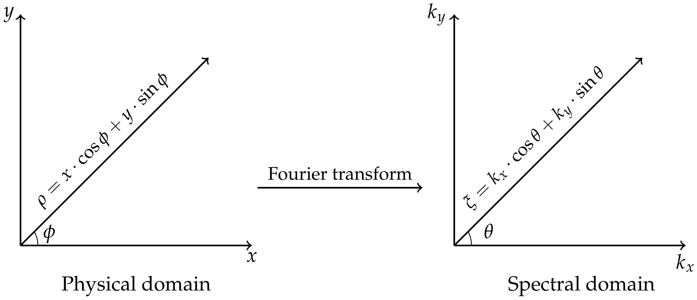
We consider $\widehat{\mathit{H}}$ to be the 2D Fourier transform of $\mathcal{H}$ along x and y directions, where the material properties are homogeneous. We have:

$$\mathcal{H}(\mathit{x},z)=\frac{1}{4{\pi }^2}{\int }_{-\infty }^{+\infty }{\int }_{-\infty }^{+\infty }\widehat{\mathit{H}}(\mathit{k},z)e^{i\mathit{k}·\mathit{x}}d\mathit{k},$$

(7)

where $\mathit{x}=(x,y)$ and $\mathit{k}=(k_x,k_y)$ (see Figure 1). We switch from the Cartesian system of coordinates to a cylindrical one according to the following transformations:

$$\begin{array}{c}x=\rho ·\cos \varphi ,y=\rho ·\sin \varphi ,\hfill \\ k_x=\xi ·\cos \theta ,k_y=\xi ·\sin \theta .\hfill \end{array}$$

(8)

Substituting (8) into (7) and applying the change of coordinates under the integral signs, we obtain:

$$\mathcal{H}\left(\mathbf{\rho }\right)=\frac{1}{4{\pi }^2}{\int }_0^{+\infty }{\int }_0^{2\pi }\widehat{\mathit{H}}(\xi ,\theta ,z)e^{i\xi \rho (\cos \theta \cos \varphi +\sin \theta \sin \varphi )}d\theta \xi d\xi ,$$

(9)

where $\mathbf{\rho }=(\rho ,\varphi ,z)$. Using the trigonometric identity:

$$\cos (\varphi -\theta )=\cos \theta \cos \varphi +\sin \theta \sin \varphi ,$$

(10)

We obtain:

$$\mathcal{H}\left(\rho \right)=\frac{1}{4{\pi }^2}{\int }_0^{+\infty }{\int }_0^{2\pi }\widehat{\mathit{H}}(\xi ,\theta ,z)e^{i\xi \rho \cos (\varphi -\theta )}d\theta \xi d\xi .$$

(11)

We now use the following relation between exponentials and Bessel functions:

$${\displaystyle e^{i\xi \rho \cos (\varphi -\theta )}=\sum _{m=-\infty }^{\infty }{i}^m{J}_m\left(\xi \rho \right)e^{-im(\varphi -\theta )}}$$

(12)

to obtain

$${\displaystyle \mathcal{H}\left(\mathbf{\rho }\right)=\frac{1}{2\pi }\sum _{m=-\infty }^{\infty }{\int }_0^{+\infty }{\mathit{H}}^m(\xi ,z)J_m\left(\xi \rho \right)e^{-im\varphi }\xi d\xi ,}$$

(13)

where

$${\mathit{H}}^m(\xi ,z)=\frac{1}{2\pi }{\int }_0^{2\pi }\widehat{\mathit{H}}(\xi ,\theta ,z)i^m{e}^{im\theta }d\theta .$$

(14)

We compute the cylindrical components of the magnetic field as follows:

$$\begin{array}{cc}\hfill H_{\rho }^m& =\cos \varphi ·H_x^m+\sin \varphi ·H_y^m\hfill \\ & =e^{i\varphi }\left(\frac{H_x^m-i{H}_y^m}{2}\right)+e^{-i\varphi }\left(\frac{H_x^m+i{H}_y^m}{2}\right)\hfill \\ & =e^{i\varphi }{H}_{+}^m+e^{-i\varphi }{H}_{-}^m,\hfill \end{array}$$

(15)

where

$$\begin{array}{cc}\hfill H_{+}^m& =\frac{H_x^m-i{H}_y^m}{2},\hfill \\ \hfill H_{-}^m& =\frac{H_x^m+i{H}_y^m}{2}.\hfill \end{array}$$

(16)

Similarly for ${\mathcal{H}}_{\varphi }$, we have:

$$\begin{array}{c}\hfill H_{\varphi }^m=-\sin \varphi ·H_x^m+\cos \varphi ·H_y^m=i\left(e^{i\varphi }{H}_{+}^m-e^{-i\varphi }{H}_{-}^m\right).\end{array}$$

(17)

By substituting (15) and (17) into (13), the Hankel representation of the magnetic field becomes:

$$\begin{array}{c}{\mathcal{H}}_{\rho }\left(\rho \right)=\frac{1}{2\pi }\sum _{m=-\infty }^{+\infty }{e}^{-im\varphi }{\int }_0^{+\infty }\left(H_{+}^m(\xi ,z)J_{m+1}\left(\xi \rho \right)+H_{-}^m(\xi ,z)J_{m-1}\left(\xi \rho \right)\right)\xi d\xi ,\hfill \\ {\mathcal{H}}_{\varphi }\left(\rho \right)=\frac{i}{2\pi }\sum _{m=-\infty }^{+\infty }{e}^{-im\varphi }{\int }_0^{+\infty }\left(H_{+}^m(\xi ,z)J_{m+1}\left(\xi \rho \right)-H_{-}^m(\xi ,z)J_{m-1}\left(\xi \rho \right)\right)\xi d\xi ,\hfill \\ {\mathcal{H}}_z\left(\rho \right)=\frac{1}{2\pi }\sum _{m=-\infty }^{+\infty }{e}^{-im\varphi }{\int }_0^{+\infty }{H}_z^m(\xi ,z)J_m\left(\xi \rho \right)\xi d\xi .\hfill \end{array}$$

(18)

The curl of the magnetic field in cylindrical coordinates is:

$$\begin{array}{cc}\hfill \nabla \times \mathcal{H}=& \left(\frac{1}{\rho }\frac{\partial {\mathcal{H}}_z}{\partial \varphi }-\frac{\partial {\mathcal{H}}_{\varphi }}{\partial z}\right)\widehat{\mathbf{\rho }}+\left(\frac{\partial {\mathcal{H}}_{\rho }}{\partial z}-\frac{\partial {\mathcal{H}}_z}{\partial \rho }\right)\widehat{\mathbf{\varphi }}+\frac{1}{\rho }\left({\mathcal{H}}_{\varphi }+\rho \frac{\partial {\mathcal{H}}_{\varphi }}{\partial \rho }-\frac{\partial {\mathcal{H}}_{\rho }}{\partial \varphi }\right)\widehat{\mathit{z}}.\hfill \end{array}$$

(19)

By substituting (18) into (19), the first component of the curl becomes:

$$\begin{array}{cc}\hfill {\left(\nabla \times \mathcal{H}\right)}_{\rho }=\frac{-i}{2\pi }\sum _{m=-\infty }^{+\infty }& e^{-im\varphi }{\int }_{\xi }(\frac{m}{\rho }{H}_z^m(\xi ,z)J_m\left(\xi \rho \right)\hfill \\ & +\frac{\partial H_{+}^m(\xi ,z)}{\partial z}{J}_{m+1}\left(\xi \rho \right)-\frac{\partial H_{-}^m(\xi ,z)}{\partial z}{J}_{m-1}\left(\xi \rho \right))\xi d\xi .\hfill \end{array}$$

(20)

By using the property of Bessel functions given by Equation (A6) of Appendix A, we obtain:

$$\begin{array}{cc}\hfill {\left(\nabla \times \mathcal{H}\right)}_{\rho }=\frac{-i}{2\pi }\sum _{m=-\infty }^{+\infty }{e}^{-im\varphi }{\int }_{\xi }[& H_z^m(\xi ,z)\left(\xi J_{m-1}\left(\xi \rho \right)-\xi \frac{\partial J_m\left(\xi \rho \right)}{\partial \left(\xi \rho \right)}\right)\hfill \\ \hfill +\frac{\partial H_{+}^m(\xi ,z)}{\partial z}& J_{m+1}\left(\xi \rho \right)-\frac{\partial H_{-}^m(\xi ,z)}{\partial z}{J}_{m-1}\left(\xi \rho \right)]\xi d\xi .\hfill \end{array}$$

(21)

Using the formula of the derivative of the Bessel function given by Equation (A4) of Appendix A, we have:

$$\begin{array}{cc}\hfill {\left(\nabla \times \mathcal{H}\right)}_{\rho }=\frac{-i}{2\pi }\sum _{m=-\infty }^{+\infty }{e}^{-im\varphi }{\int }_{\xi }\left[H_z^m(\xi ,z)\right(& \xi J_{m-1}\left(\xi \rho \right)-\frac{\xi }{2}{J}_{m-1}\left(\xi \rho \right)+\frac{\xi }{2}{J}_{m+1}\left(\xi \rho \right))\hfill \\ \hfill +\frac{\partial H_{+}^m(\xi ,z)}{\partial z}{J}_{m+1}\left(\xi \rho \right)-& \frac{\partial H_{-}^m(\xi ,z)}{\partial z}{J}_{m-1}\left(\xi \rho \right)]\xi d\xi .\hfill \end{array}$$

(22)

For an arbitrary function $\mathbf{g}(\xi ,z)=(g_{-}(\xi ,z),g_{+}(\xi ,z),g_z(\xi ,z))$ in the spectral domain, we introduce the following notation to simplify computations:

$$\begin{array}{c}{\Pi }_{+}^{\xi }\left(\mathbf{g}(\xi ,z)\right)=\frac{\partial g_{+}(\xi ,z)}{\partial z}+\frac{\xi }{2}{g}_z(\xi ,z),\hfill \\ {\Pi }_{-}^{\xi }\left(\mathbf{g}(\xi ,z)\right)=\frac{\partial g_{-}(\xi ,z)}{\partial z}-\frac{\xi }{2}{g}_z(\xi ,z),\hfill \\ {\Pi }_z^{\xi }\left(\mathbf{g}(\xi ,z)\right)=\xi \left(g_{-}(\xi ,z)+g_{+}(\xi ,z)\right).\hfill \end{array}$$

(23)

Using (23), we obtain:

$$\begin{array}{cc}\hfill {\left(\nabla \times \mathcal{H}\right)}_{\rho }=-\frac{i}{2\pi }\sum _{m=-\infty }^{+\infty }{e}^{-im\varphi }{\int }_{\xi }(& {\Pi }_{+}^{\xi }\left({\mathbf{H}}^m(\xi ,z)\right)J_{m+1}\left(\xi \rho \right)-{\Pi }_{-}^{\xi }\left({\mathbf{H}}^m(\xi ,z)\right)J_{m-1}\left(\xi \rho \right))\xi d\xi .\hfill \end{array}$$

(24)

For the second component of (19), using (18), we have:

$$\begin{array}{cc}\hfill {\left(\nabla \times \mathcal{H}\right)}_{\varphi }=\frac{1}{2\pi }\sum _{m=-\infty }^{+\infty }{e}^{-im\varphi }{\int }_{\xi }[& (\frac{\partial H_{+}^m(\xi ,z)}{\partial z}{J}_{m+1}\left(\xi \rho \right)\hfill \\ \hfill +\frac{\partial H_{-}^m(\xi ,z)}{\partial z}& J_{m-1}\left(\xi \rho \right))-H_z^m(\xi ,z)\frac{\partial J_{m+1}\left(\xi \rho \right)}{\partial \left(\xi \rho \right)}\xi ]\xi d\xi .\hfill \end{array}$$

(25)

Using the property of the Bessel functions given by Equation (A4) of Appendix A and (23), we obtain:

$$\begin{array}{cc}\hfill {\displaystyle {\left(\nabla \times \mathcal{H}\right)}_{\varphi }=\frac{1}{2\pi }\sum _{m=-\infty }^{+\infty }{e}^{-im\varphi }{\int }_{\xi }(}& {\Pi }_{+}^{\xi }\left({\mathbf{H}}^m(\xi ,z)\right)J_{m+1}\left(\xi \rho \right)+{\Pi }_{-}^{\xi }\left({\mathbf{H}}^m(\xi ,z)\right)J_{m-1}\left(\xi \rho \right))\xi d\xi .\hfill \end{array}$$

(26)

The third component of (19), becomes after using (18):

$$\begin{array}{cc}\hfill {\left(\nabla \times \mathcal{H}\right)}_z=\frac{i}{2\pi }\sum _{m=-\infty }^{+\infty }{e}^{-im\varphi }·{\int }_{\xi }& [\left(\frac{J_{m+1}\left(\xi \rho \right)}{\rho }+\xi \frac{\partial J_{m+1}\left(\xi \rho \right)}{\partial \left(\xi \rho \right)}+\frac{m}{\rho }{J}_{m+1}\left(\xi \rho \right)\right)H_{+}^m(\xi ,z)\hfill \\ & -\left(\frac{J_{m-1}\left(\xi \rho \right)}{\rho }+\xi \frac{\partial J_{m-1}\left(\xi \rho \right)}{\partial \left(\xi \rho \right)}-\frac{m}{\rho }{J}_{m-1}\left(\xi \rho \right)\right)H_{-}^m(\xi ,z)]\xi d\xi .\hfill \end{array}$$

(27)

For the derivative of $J_{m+1}$, we use Equation (A6) of Appendix A, and for the derivative of $J_{m-1}$, we use Equation (A4) of the same appendix. Then,

$$\begin{array}{cc}\hfill {\left(\nabla \times \mathcal{H}\right)}_z=\frac{i}{2\pi }\sum _{m=-\infty }^{+\infty }{e}^{-im\varphi }{\int }_{\xi }[& \left(\frac{J_{m+1}\left(\xi \rho \right)}{\rho }+\xi J_m\left(\xi \rho \right)-\frac{m+1}{\rho }{J}_{m+1}\left(\xi \rho \right)+\frac{m}{\rho }{J}_{m+1}\left(\xi \rho \right)\right)H_{+}^m(\xi ,z)\hfill \\ & -\left(\frac{J_{m-1}\left(\xi \rho \right)}{\rho }+\frac{\xi }{2}{J}_{m-2}\left(\xi \rho \right)-\frac{\xi }{2}{J}_m\left(\xi \rho \right)-\frac{m}{\rho }{J}_{m-1}\left(\xi \rho \right)\right)H_{-}^m(\xi ,z)]\xi d\xi .\hfill \end{array}$$

(28)

We use Equation (A1) of Appendix A to simplify $J_{m-2}$. As a result, we obtain:

$$\begin{array}{c}\hfill {\left(\nabla \times \mathcal{H}\right)}_z=\frac{i}{2\pi }\sum _{m=-\infty }^{+\infty }{e}^{-im\varphi }{\int }_{\xi }{\Pi }_z^{\xi }\left({\mathbf{H}}^m(\xi ,z)\right)J_m\left(\xi \rho \right)\xi d\xi .\end{array}$$

(29)

3.2. Hankel Finite Element (HFE) Full Field Formulation

$L^2$-orthogonality holds for Bessel functions of with the same order (see Equation (A3) of Appendix A). Hence, in order to simplify the terms of the variational formulation containing Bessel functions, we introduce the following matrix:

$${\displaystyle Q=\frac{1}{\sqrt{2}}\left(\begin{array}{ccc}1& i& 0\\ i& 1& 0\\ 0& 0& \sqrt{2}\end{array}\right).}$$

(30)

Q is a unitary matrix, since:

$$Q{Q}^{*}=Q^{*}Q=I.$$

Hence, the change of coordinates implied by Q preserves the inner product. In particular, for arbitrary vector-valued functions $\mathbf{U}$ and $\mathbf{V}$, we have:

$${\mathbf{V}}^{*}\mathbf{U}={\left(Q\mathbf{V}\right)}^{*}\left(Q\mathbf{U}\right).$$

By using the above matrix, we obtain the following equalities:

$$\begin{array}{cc}\hfill {\displaystyle {\left(Q{\tilde{\sigma }}^{-1}\left(z\right)\nabla \times \mathcal{H}\right)}_{\rho }=\frac{i}{\sqrt{2}\pi }\sum _{m=-\infty }^{+\infty }}& e^{-im\varphi }{\int }_0^{+\infty }{\tilde{\sigma }}_h^{-1}\left(z\right)·{\Pi }_{-}^{\xi }\left({\mathbf{H}}^m(\xi ,z)\right)J_{m-1}\left(\xi \rho \right)\xi d\xi ,\hfill \\ \hfill {\left(Q{\tilde{\sigma }}^{-1}\left(z\right)\nabla \times \mathcal{H}\right)}_{\varphi }=\frac{1}{\sqrt{2}\pi }\sum _{m=-\infty }^{+\infty }& e^{-im\varphi }{\int }_0^{+\infty }{\tilde{\sigma }}_h^{-1}\left(z\right)·{\Pi }_{+}^{\xi }\left({\mathbf{H}}^m(\xi ,z)\right)J_{m+1}\left(\xi \rho \right)\xi d\xi ,\hfill \\ \hfill {\left(Q{\tilde{\sigma }}^{-1}\left(z\right)\nabla \times \mathcal{H}\right)}_z=\frac{i}{2\pi }\sum _{m=-\infty }^{+\infty }& e^{-im\varphi }{\int }_0^{+\infty }{\tilde{\sigma }}_v^{-1}\left(z\right)·{\Pi }_z^{\xi }\left({\mathbf{H}}^m(\xi ,z)\right)J_m\left(\xi \rho \right)\xi d\xi ,\hfill \end{array}$$

(31)

where ${\tilde{\sigma }}_h={\sigma }_h-i\omega {\epsilon }_h$ and ${\tilde{\sigma }}_v={\sigma }_v-i\omega {\epsilon }_v$. For the $L^2$ terms, we obtain:

$$\begin{array}{cc}\hfill {\left(Q\mathcal{H}\right)}_{\rho }& =\frac{1}{\sqrt{2}\pi }\sum _{m=-\infty }^{+\infty }{e}^{-im\varphi }{\int }_0^{+\infty }{H}_{-}^m(\xi ,z)J_{m-1}\left(\xi \rho \right)\xi d\xi ,\hfill \\ \hfill {\left(Q\mathcal{H}\right)}_{\varphi }& =\frac{i}{\sqrt{2}\pi }\sum _{m=-\infty }^{+\infty }{e}^{-im\varphi }{\int }_0^{+\infty }{H}_{+}^m(\xi ,z)J_{m+1}\left(\xi \rho \right)\xi d\xi ,\hfill \\ \hfill {\left(Q\mathcal{H}\right)}_z& =\frac{1}{2\pi }\sum _{m=-\infty }^{+\infty }{e}^{-im\varphi }{\int }_0^{+\infty }{H}_z^m(\xi ,z)J_m\left(\xi \rho \right)\xi d\xi .\hfill \end{array}$$

(32)

For a specific Hankel mode ${\xi }_q>0$ and an exponential order t, we select a mono-modal test function of the form:

$${\mathcal{F}}^{q,t}\left(\mathbf{\rho }\right)={\mathcal{F}}_{\rho }^{q,t}\left(\mathbf{\rho }\right)\widehat{\mathbf{\rho }}+{\mathcal{F}}_{\varphi }^{q,t}\left(\mathbf{\rho }\right)\widehat{\mathbf{\varphi }}+{{F}}_z^{q,t}\left(\mathbf{\rho }\right)\widehat{\mathbf{z}},$$

(33)

where:

$$\begin{array}{c}{\mathcal{F}}_{\rho }^{q,t}\left(\mathbf{\rho }\right)=e^{-it\varphi }\left(F_{+}^t({\xi }_q,z)J_{t+1}\left({\xi }_q\rho \right)+F_{-}^t({\xi }_q,z)J_{t-1}\left({\xi }_q\rho \right)\right),\hfill \\ {{F}}_{\varphi }^{q,t}\left(\mathbf{\rho }\right)=i{e}^{-it\varphi }\left(F_{+}^t({\xi }_q,z)J_{t+1}\left({\xi }_q\rho \right)-F_{-}^t({\xi }_q,z)J_{t-1}\left({\xi }_q\rho \right)\right),\hfill \\ {\mathcal{F}}_z^{q,t}\left(\mathbf{\rho }\right)=e^{-it\varphi }{F}_z^t({\xi }_q,z)J_t\left({\xi }_q\rho \right).\hfill \end{array}$$

(34)

Using (31) and the test functions defined in (34), we have:

$$\begin{array}{cc}\hfill {\int }_{z,\varphi ,\rho }& {\left(Q\nabla \times {\mathcal{F}}^{q,t}\right)}_{\rho }^{*}{\left(Q{\tilde{\sigma }}^{-1}\left(z\right)\nabla \times \mathcal{H}\right)}_{\rho }\rho d\rho d\varphi dz=\frac{1}{\pi }{\int }_z(\sum _{m=-\infty }^{+\infty }{\int }_{\xi ,\varphi ,\rho }{e}^{i(t-m)\varphi }\hfill \\ & ·{\left({\Pi }_{-}^{{\xi }_q}\left({\mathbf{F}}^t\right)\right)}^{*}{\tilde{\sigma }}_h^{-1}\left(z\right){\Pi }_{-}^{\xi }\left({\mathbf{H}}^m\right)·J_{t-1}\left({\xi }_q\rho \right)J_{m-1}\left(\xi \rho \right)\rho d\rho d\varphi \xi d\xi )dz,\hfill \end{array}$$

(35)

where ${\mathbf{F}}^t=(F_{+}^t,F_{-}^t,F_z^t)$. Separating the integrals according to each variable and using the $L^2$-orthogonality property of exponential functions, we have:

$$\begin{array}{cc}\hfill {\int }_{z,\varphi ,\rho }{\left(Q\nabla \times {\mathcal{F}}^{q,t}\right)}_{\rho }^{*}& {\left(Q{\tilde{\sigma }}^{-1}\left(z\right)\nabla \times \mathcal{H}\right)}_{\rho }\rho d\rho d\varphi dz\hfill \\ \hfill =2{\int }_z\left[{\int }_{\xi }\right(& {\left({\Pi }_{-}^{{\xi }_q}\left({\mathbf{F}}^t\right)\right)}^{*}{\tilde{\sigma }}_h^{-1}\left(z\right){\Pi }_{-}^{\xi }\left({\mathbf{H}}^t\right)·{\int }_{\rho }{J}_{t-1}\left({\xi }_q\rho \right)J_{t-1}\left(\xi \rho \right)\rho d\rho \left)\xi d\xi \right]dz.\hfill \end{array}$$

(36)

By the orthogonality property of the Bessel functions given by Equation (A3) of Appendix A, we obtain:

$$\begin{array}{cc}\hfill {\int }_{z,\varphi ,\rho }{\left(Q\nabla \times {\mathcal{F}}^{q,t}\right)}_{\rho }^{*}& {\left(Q{\tilde{\sigma }}^{-1}\left(z\right)\nabla \times \mathcal{H}\right)}_{\rho }\rho d\rho d\varphi dz=2{\int }_z{\left({\Pi }_{-}^{{\xi }_q}\left({\mathbf{F}}^t\right)\right)}^{*}{\tilde{\sigma }}_h^{-1}\left(z\right){\Pi }_{-}^{{\xi }_q}\left({\mathbf{H}}^t\right)dz.\hfill \end{array}$$

(37)

Similarly, for the other components of the curl, we have:

$$\begin{array}{cc}\hfill {\int }_{z,\varphi ,\rho }{\left(Q\nabla \times {\mathcal{F}}^{q,t}\right)}_{\varphi }^{*}& {\left(Q{\tilde{\sigma }}^{-1}\left(z\right)\nabla \times \mathcal{H}\right)}_{\varphi }\rho d\rho d\varphi dz=2{\int }_z{\left({\Pi }_{+}^{{\xi }_q}\left({\mathbf{F}}^t\right)\right)}^{*}{\tilde{\sigma }}_h^{-1}\left(z\right){\Pi }_{+}^{{\xi }_q}\left({\mathbf{H}}^t\right)dz,\hfill \end{array}$$

(38)

$$\begin{array}{cc}\hfill {\int }_{z,\varphi ,\rho }{\left(Q\nabla \times {\mathcal{F}}^{q,t}\right)}_z^{*}& {\left(Q{\tilde{\sigma }}^{-1}\left(z\right)\nabla \times \mathcal{H}\right)}_z\rho d\rho d\varphi dz={\int }_z{\left({\Pi }_z^{{\xi }_q}\left({\mathbf{F}}^t\right)\right)}^{*}{\tilde{\sigma }}_v^{-1}\left(z\right){\Pi }_z^{{\xi }_q}\left({\mathbf{H}}^t\right)dz.\hfill \end{array}$$

(39)

For the $L^2$ terms, using (32) and the test functions defined in (34), and using $L^2$-orthogonality property of exponentials and orthogonality property of the Bessel functions given by (A3) of Appendix A, we obtain:

$$\begin{array}{c}{\int }_{z,\varphi ,\rho }{\left(Q{\mathcal{F}}^{q,t}\right)}_{\rho }^{*}{\left(Q\mathbf{\mu }\mathcal{H}\right)}_{\rho }\rho d\rho d\varphi dz=2{\int }_z{\left(F_{-}^t({\xi }_q,z)\right)}^{*}{\mu }_h\left(z\right)H_{-}^t({\xi }_q,z)dz,\hfill \\ {\int }_{z,\varphi ,\rho }{\left(Q{\mathcal{F}}^{q,t}\right)}_{\varphi }^{*}{\left(Q\mathbf{\mu }\mathcal{H}\right)}_{\varphi }\rho d\rho d\varphi dz=2{\int }_z{\left(F_{+}^t({\xi }_q,z)\right)}^{*}{\mu }_h\left(z\right)H_{+}^t({\xi }_q,z)dz,\hfill \\ {\int }_{z,\varphi ,\rho }{\left(Q{\mathcal{F}}^{q,t}\right)}_z^{*}{\left(Q\mathbf{\mu }\mathcal{H}\right)}_z\rho d\rho d\varphi dz={\int }_z{\left(F_z^t({\xi }_q,z)\right)}^{*}{\mu }_v\left(z\right)H_z^t({\xi }_q,z)dz.\hfill \end{array}$$

(40)

Using (37)–(40), for each Hankel mode ${\xi }_q>0$ and exponential order t, the stiffness matrix becomes:

$$b({\mathcal{F}}^{q,t},\mathcal{H})=b({\mathbf{F}}^t,{\mathbf{H}}^t)=b_1({\mathbf{F}}^t,{\mathbf{H}}^t)-b_2({\mathbf{F}}^t,{\mathbf{H}}^t),$$

(41)

where

$$\begin{array}{cc}\hfill b_1({\mathbf{F}}^t,{\mathbf{H}}^t)=& 2{\langle {\Pi }_{-}^{{\xi }_q}\left({\mathbf{F}}^t\right),{\tilde{\sigma }}_h^{-1}{\Pi }_{-}^{{\xi }_q}\left({\mathbf{H}}^t\right)\rangle }_{L^2}+2{\langle {\Pi }_{+}^{{\xi }_q}\left({\mathbf{F}}^t\right),{\tilde{\sigma }}_h^{-1}{\Pi }_{+}^{{\xi }_q}\left({\mathbf{H}}^t\right)\rangle }_{L^2}+{\langle {\Pi }_z^{{\xi }_q}\left({\mathbf{F}}^t\right),{\tilde{\sigma }}_v^{-1}{\Pi }_z^{{\xi }_q}\left({\mathbf{H}}^t\right)\rangle }_{L^2},\hfill \\ \hfill b_2({\mathbf{F}}^t,{\mathbf{H}}^t)=& i\omega \left(2{\langle F_{-}^t,{\mu }_h{H}_{-}^t\rangle }_{L^2}+2{\langle F_{+}^t,{\mu }_h{H}_{+}^t\rangle }_{L^2}+{\langle F_z^t,{\mu }_v{H}_z^t\rangle }_{L^2}\right).\hfill \end{array}$$

(42)

Symbol $<.,.{>}_{L^2}$ represents the $L^2$ inner product given by:

$${\langle f,g\rangle }_{L^2}={\int }_z{f}^{*}gdz.$$

A sufficient condition to guarantee that the above integrals are finite is to require ${\mathbf{H}}^t,{\mathbf{F}}^t\in V\left(\mathbb{R}\right)$, where $V\left(\mathbb{R}\right)=H^1\left(\mathbb{R}\right)\times H^1\left(\mathbb{R}\right)\times L^2\left(\mathbb{R}\right)$, and

$$H^1\left(\mathbb{R}\right)=\{v\in L^2\left(\mathbb{R}\right):\frac{\partial v}{\partial z}\in L^2\left(\mathbb{R}\right)\}.$$

(43)

In (43), the weak derivative of the function is considered.

Load vector

In 1D layered medium, we consider $(0,0,z_{Tx})$ to be the general representation of a point source location. We use the following identities to describe the right-hand-side vector in cylindrical coordinates:

$$\begin{array}{cc}\hfill \widehat{\mathit{x}}& =\cos \left(\varphi \right)\widehat{\mathbf{\rho }}-\sin \left(\varphi \right)\widehat{\mathbf{\varphi }}=\frac{e^{-i\varphi }}{2}(\widehat{\mathbf{\rho }}-i\widehat{\mathbf{\varphi }})+\frac{e^{i\varphi }}{2}(\widehat{\mathbf{\rho }}+i\widehat{\mathbf{\varphi }}),\hfill \\ \hfill \widehat{\mathit{y}}& =\sin \left(\varphi \right)\widehat{\mathbf{\rho }}+\cos \left(\varphi \right)\widehat{\mathbf{\varphi }}=\frac{e^{-i\varphi }}{2}(i\widehat{\mathbf{\rho }}+\widehat{\mathbf{\varphi }})-\frac{e^{i\varphi }}{2}(i\widehat{\mathbf{\rho }}-\widehat{\mathbf{\varphi }}),\hfill \\ \hfill \widehat{\mathit{z}}& =\widehat{\mathit{z}},\hfill \end{array}$$

(44)

where $\widehat{\mathit{x}}$, $\widehat{\mathit{y}}$ and $\widehat{\mathit{z}}$ are the unitary vectors in Cartesian coordinates. The right-hand-side of (3) in cylindrical coordinates for a z-oriented point source is:

$${\mathbf{R}}_z=i\omega {\mu }_v\left(z\right)\frac{1}{2\pi \rho }\delta (\rho ,0)\delta (z,z_{Tx})\widehat{\mathbf{z}},$$

where $\delta$ is the Dirac delta distribution. We consider l to be the right-hand-side of (5). Using ${\mathcal{F}}^{q,t}$ as our test function and separating the integrals according to each variable, we obtain:

$$\begin{array}{cc}\hfill l\left({\mathbf{F}}^t\right)=& \frac{i\omega }{2\pi }{\int }_{\varphi =0}^{2\pi }{e}^{it\varphi }d\varphi {\int }_{\rho =0}^{+\infty }{J}_t\left({\xi }_q\rho \right)\delta (\rho ,0)\rho d\rho \hfill \\ & ·{\int }_{z=-\infty }^{+\infty }{\mu }_v\left(z\right){\left(F_z^t({\xi }_q,z)\right)}^{*}\delta (z,z_{Tx})dz.\hfill \end{array}$$

(45)

By $L^2$-orthogonality of the exponentials, the load vector is non-zero when $t=0$. Since $J_0\left(0\right)=1$, for a z-oriented point source, the right-hand-side becomes:

$$l\left({\mathbf{F}}^0\right)=i\omega {\mu }_v\left(z_{Tx}\right){\left(F_z^0({\xi }_q,z_{Tx})\right)}^{*}.$$

(46)

Hence, we obtain the field by solving the following variational formulation:

$$\begin{array}{cc}\hfill b& ({\mathbf{F}}^0,{\mathbf{H}}^0)=l\left({\mathbf{F}}^0\right),\mathrm{for}\mathrm{all}{\mathbf{F}}^0\in V\left(\mathbb{R}\right).\hfill \end{array}$$

(47)

Lets consider ${\mathbf{R}}_x$ and ${\mathbf{R}}_y$ to be the right-hand-sides of (3) for x and y-oriented sources, respectively. By using (44), we obtain:

$$\begin{array}{cc}\hfill {\mathbf{R}}_x=\underset{{\rho }_{Tx}\to 0^{+}}{lim}& \frac{i\omega {\mu }_h\left(z\right)}{2\pi \rho }\delta (\rho ,{\rho }_{Tx})\delta (z,z_{Tx})\left(\frac{e^{-i\varphi }}{2}(\widehat{\mathbf{\rho }}-i\widehat{\mathbf{\varphi }})+\frac{e^{i\varphi }}{2}(\widehat{\mathbf{\rho }}+i\widehat{\mathbf{\varphi }})\right),\hfill \\ \hfill {\mathbf{R}}_y=\underset{{\rho }_{Tx}\to 0^{+}}{lim}& \frac{i\omega {\mu }_h\left(z\right)}{2\pi \rho }\delta (\rho ,{\rho }_{Tx})\delta (z,z_{Tx})\left(\frac{e^{-i\varphi }}{2}(i\widehat{\mathbf{\rho }}+\widehat{\mathbf{\varphi }})-\frac{e^{i\varphi }}{2}(i\widehat{\mathbf{\rho }}-\widehat{\mathbf{\varphi }})\right).\hfill \end{array}$$

(48)

Similarly to (46), the right-hand-side of the variational formulation is non-zero only when $t=-1,1$. For those values of t, and for each Hankel mode, we have:

$$b({\mathbf{F}}^t,{\mathbf{H}}^t)=\underset{{\rho }_{Tx}\to 0+}{lim}l\left({\mathbf{F}}^t\right),\mathrm{for}\mathrm{all}{\mathbf{F}}^t\in V\left(\mathbb{R}\right),$$

(49)

where,

$$\begin{array}{cc}\hfill l\left({\mathbf{F}}^t\right)=& i\omega {\mu }_h\left(z_{Tx}\right)[\frac{F_{+}^t({\xi }_q,z_{Tx})}{2}{J}_{t+1}\left({\xi }_q{\rho }_{Tx}\right)+\frac{F_{-}^t({\xi }_q,z_{Tx})}{2}{J}_{t-1}\left({\xi }_q{\rho }_{Tx}\right)\hfill \\ & -t\left(\frac{F_{+}^t({\xi }_q,z_{Tx})}{2}{J}_{t+1}\left({\xi }_q{\rho }_{Tx}\right)-\frac{F_{-}^t({\xi }_q,z_{Tx})}{2}{J}_{t-1}\left({\xi }_q{\rho }_{Tx}\right)\right){]}^{*}\hfill \\ & =i\omega {\mu }_h\left(z_{Tx}\right)J_0\left({\xi }_q{\rho }_{Tx}\right)\left\{\begin{array}{cc}{\left(F_{+}^t({\xi }_q,z_{Tx})\right)}^{*},\hfill & t=-1,\hfill \\ {\left(F_{-}^t({\xi }_q,z_{Tx})\right)}^{*},\hfill & t=1.\hfill \end{array}\right.\hfill \end{array}$$

(50)

Based on (18), we define the following notation:

$$\begin{array}{c}{\mathcal{H}}_{\rho }^t\left(\mathbf{\rho }\right)=\frac{1}{2\pi }{e}^{-it\varphi }{\int }_{\xi =0}^{+\infty }\left(H_{+}^t(\xi ,z)J_{t+1}\left(\xi \rho \right)+H_{-}^t(\xi ,z)J_{t-1}\left(\xi \rho \right)\right)\xi d\xi ,\hfill \\ {\mathcal{H}}_{\varphi }^t\left(\mathbf{\rho }\right)=\frac{i}{2\pi }{e}^{-it\varphi }{\int }_{\xi =0}^{+\infty }\left(H_{+}^t(\xi ,z)J_{t+1}\left(\xi \rho \right)-H_{-}^t(\xi ,z)J_{t-1}\left(\xi \rho \right)\right)\xi d\xi ,\hfill \\ {\mathcal{H}}_z^t\left(\mathbf{\rho }\right)=\frac{1}{2\pi }{e}^{-it\varphi }{\int }_{\xi =0}^{+\infty }{H}_z^t(\xi ,z)J_t\left(\xi \rho \right)\xi d\xi .\hfill \end{array}$$

(51)

We have ${\mathcal{H}}^t=({\mathcal{H}}_{\rho }^t,{\mathcal{H}}_{\varphi }^t,{\mathcal{H}}_z^t)$. Therefore, the magnetic field for the x-oriented source is:

$$\mathcal{H}={\mathcal{H}}^1+{\mathcal{H}}^{-1}.$$

(52)

For a y-oriented source, the field is computed as:

$$\mathcal{H}=i{\mathcal{H}}^1-i{\mathcal{H}}^{-1}.$$

(53)

4. Multi-Scale Hankel Finite Element Method (Ms-HFEM)

We now describe our multi-scale FE method in the Hankel domain. In order to make the computational problem tractable, we truncate our domain along the z direction. We consider ${\Omega }_z=(z_0,z_N)$ to be our problem domain along z direction and we have $-\infty <z_0$ and $z_N<\infty$. Moreover, we consider our solution to satisfy a zero Dirichlet boundary condition at both ends, since the waves amplitude rapidly decreases as we move away from the source. Thus, we have ${\mathbf{H}}^m,{\mathbf{F}}^m\in V_0\left({\Omega }_z\right)$, where $V_0\left({\Omega }_z\right)=H_0^1\left({\Omega }_z\right)\times H_0^1\left({\Omega }_z\right)\times L^2\left({\Omega }_z\right)$, with:

$$H_0^1\left({\Omega }_z\right)=\{v\in H^1\left({\Omega }_z\right),v\left(z_i\right)=0\mathrm{for}{z}_i\in \partial {\Omega }_z\}.$$

(54)

In the following, for simplicity, we shall remove symbols ${\xi }_q$ and t from the notation. For each Hankel mode, we need to solve three problems associated with $t=-1,0,1$. The curl operator is the one defined in (24), (26) and (29). Similarly, ${\Pi }_{+}$, ${\Pi }_{-}$, and ${\Pi }_z$ are the symbols defined in Equation (23), and l is the right-hand-side of the variational formulation described in Equations (46) and (50) for $t=-1,0,1$. Our multi-scale approach consists of the following steps for each Hankel mode:

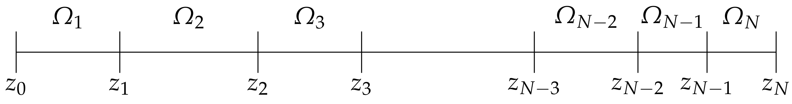
• Divide the domain into a finite number of sub-domains. We consider $z_0,z_1,z_2,\cdots ,z_{N-1},z_N$, where $z_1,z_2,\cdots ,z_{N-1}$ are arbitrary real numbers and $z_0<z_1<\cdots <z_N$ (see Figure 2). We call them decomposition points. We define each sub-domain as ${\Omega }_i=(z_{i-1},z_i)$, and we have:

  $$\overline{{\Omega }_z}=\bigcup _{i=1}^N\overline{{\Omega }_i}.$$

  (55)
• Decompose the magnetic field into primary and secondary fields. For each Hankel mode, we decompose our magnetic field as follows:

  $$\mathbf{H}\left(z\right)={\mathbf{H}}^P\left(z\right)+{\mathbf{H}}^S\left(z\right),$$

  (56)

  where ${\mathbf{H}}^P$ and ${\mathbf{H}}^S$ are primary and secondary fields, respectively.
• Find a local primary field. Lets assume that $z_{Tx}\in {\Omega }_p$ (see Figure 3). We define our local primary field ${\mathbf{H}}^P\in V_0\left({\Omega }_p\right)$ as the one that satisfies:

  $$b(\mathbf{F},{\mathbf{H}}^P)=l\left(\mathbf{F}\right),\mathbf{F}\in V_0\left({\Omega }_p\right).$$

  (57)
  Extending the local primary field to the entire domain with zero, we have ${\mathbf{H}}^P\in V_0\left({\Omega }_z\right)$. The local primary field has a discontinuous flux at $z_{p-1}$ and $z_p$. For the special case when the source is located at one decomposition point, we consider $z_{Tx}=z_p^{\prime }$, where

  $$z_p^{\prime }=\left\{\begin{array}{cc}{z}_{Tx}+{10}^{-5}\mathrm{meters}\hfill & z_{Tx}=z_{p-1},\hfill \\ z_{Tx}-{10}^{-5}\mathrm{meters}\hfill & z_{Tx}=z_p.\hfill \end{array}\right.$$

  (58)
  The ${10}^{-5}$ displacement is an arbitrary choice. We use a small number compatible with our grid size, but other values are also valid.
• Solve $(N-1)$ pairs of local problems. We consider ${\Omega }_i^M={\Omega }_i\cup {\Omega }_{i+1}\cup \left\{z_i\right\}$, $i=1,\cdots ,(N-1)$. For each sub-domain ${\Omega }_i^M$, we solve a pair of local problems which correspond to a discontinuous flux at the node $z=z_i$. Specifically, the flux of the first local problem has a jump equal to ${\mathbf{1}}_1=(1,0,0)$, and the flux of the second local problem has a jump equal to ${\mathbf{1}}_2=(0,1,0)$. The local functions ${\mathbf{\psi }}^{i,k}\in V_0\left({\Omega }_i^M\right)$ solve the following variational problems:

  $$b(\mathbf{F},{\mathbf{\psi }}^{i,k})=l^{M,k}\left(\mathbf{F}\right),\mathbf{F}\in V_0\left({\Omega }_i^M\right),i=1,\cdots ,(N-1),k=1,2,$$

  (59)

  where ${\mathbf{\psi }}^{i,k}\left(z\right)=({\psi }_{-}^{i,k}\left(z\right),{\psi }_{+}^{i,k}\left(z\right),{\psi }_z^{i,k}\left(z\right))$, and $l^{M,k}$ corresponds to the jump of the flux of the solutions at $z=z_i$. Specifically:

  $$\begin{array}{c}{l}^{M,1}\left(\mathbf{F}\right)=2{\left(F_{-}\left(z_i\right)\right)}^{*},\hfill \\ l^{M,2}\left(\mathbf{F}\right)=2{\left(F_{+}\left(z_i\right)\right)}^{*},\hfill \\ \mathrm{for}i=1,\cdots ,(N-1).\hfill \end{array}$$

  (60)
  Similarly to the local primary field, we consider the extension by zero of the local solutions on ${\Omega }_z$, and we have ${\mathbf{\psi }}^{i,k}\in V_0\left({\Omega }_z\right)$. We denote the solutions of these local problems as multi-scale basis functions. We define the following space of multi-scale basis functions:

  $$V_M=\mathrm{span}{\left\{{\left\{{\mathbf{\psi }}^{i,k}\left(z\right)=\left({\psi }_{-}^{i,k}\left(z\right),{\psi }_{+}^{i,k}\left(z\right),{\psi }_z^{i,k}\left(z\right)\right)\right\}}_{i=1}^{N-1}\right\}}_{k=1}^2.$$

  (61)
• Solve the secondary field formulation using the multi-scale basis functions. Since the flux components of the local primary field are discontinuous, we need our secondary field to balance these artificial discontinuities. Thus, by combining the primary and secondary fields, we recover a continuous flux for the full field. From (56), we obtain:

  $$b(\mathbf{F},{\mathbf{H}}^S)=b(\mathbf{F},\mathbf{H})-b(\mathbf{F},{\mathbf{H}}^P)=l\left(\mathbf{F}\right)-b(\mathbf{F},{\mathbf{H}}^P),\mathbf{F}\in V_0\left({\Omega }_z\right).$$

  (62)
  We describe our secondary field as follows:

  $${\mathbf{H}}^S\left(z\right)=\sum _{i=1}^{N-1}\sum _{k=1}^2{\mathbf{\alpha }}_{i,k}{\psi }^{i,k}\left(z\right),$$

  (63)

  where ${\mathbf{H}}^S=(H_{-}^S,H_{+}^S,H_z^S)$, and ${\mathbf{\psi }}^{i,k}\in V_M$. By the definition of the multi-scale basis functions, (63) satisfies the reduced wave equation. Moreover, we consider $\mathbf{F}\in V_M$. Therefore, by substituting (63) into (62), we have:

  $$\begin{array}{cc}\hfill \sum _{i=1}^{N-1}\sum _{k=1}^2{\alpha }_{i,k}b({\mathbf{\psi }}^{m,n},{\mathbf{\psi }}^{i,k})& =l\left({\mathbf{\psi }}^{m,n}\right)-b({\mathbf{\psi }}^{m,n},{\mathbf{H}}^P),m=1,\cdots ,(N-1),n=1,2.\hfill \end{array}$$

  (64)
  Finally, we add the local primary field and the secondary field to evaluate the full field.

In the next sections, we further describe the formulation for each step.

4.1. Local Primary Field

We consider the local primary field defined in Equation (57). We further decompose our primary field as follows:

$${\mathbf{H}}^P={\mathbf{H}}^F{|}_{{\Omega }_p}+{\mathbf{H}}^C,$$

(65)

where ${\mathbf{H}}^F$ is the fundamental solution of the electromagnetic reduced wave equation, and ${\mathbf{H}}^C$ is a correction field.

Since the fundamental field has no boundary condition at the boundaries of ${\Omega }_p$, the correction field is intended to enforce the zero Dirichlet (tangential) boundary condition on ${\mathbf{H}}^P$ (see Figure 4). We define our correction field as follows:

$${\mathbf{H}}^C=\sum _{i=p-1}^p\sum _{k=1}^2{\beta }_{i,k}{\mathbf{H}}^{C,i,k},$$

(66)

where ${\mathbf{H}}^{C,i,k}$ ($i=p-1,p$ and $k=1,2$) are the correction basis functions. To define them, we perform the following decomposition:

$${\mathbf{H}}^{C,i,k}={\mathbf{H}}_0^{C,i,k}+{\mathbf{H}}_1^{C,i,k},i=p-1,p,k=1,2,$$

(67)

where ${\mathbf{H}}_0^{C,i,k}\in V_0\left({\Omega }_p\right)$, and ${\mathbf{H}}_1^{C,i,k}\in V^j\left({\Omega }_p\right)$, for $j\ne i$, is a lift of the correction field at $z_i$ to impose the non-zero Dirichlet boundary condition. $V^i\left({\Omega }_p\right)\subset V\left({\Omega }_p\right)$, for $i=p-1,p$, is the space of all vector-valued functions $\mathbf{F}\in V\left({\Omega }_p\right)$ satisfying a zero Dirichlet (tangential) boundary condition at $z=z_i$. By substituting (67) into variational formulation (41), we arrive at:

$$b(\mathbf{F},{\mathbf{H}}_0^{C,i,k})=-b(\mathbf{F},{\mathbf{H}}_1^{C,i,k}),{\mathbf{H}}_0^{C,i,k},\mathbf{F}\in V_0\left({\Omega }_p\right),i=p-1,p,k=1,2.$$

(68)

In order to impose a zero Dirichlet (tangential) boundary condition for our local primary field, we enforce the following conditions:

$${\mathbf{n}}_j\times {\mathbf{H}}^C\left(z_j\right)=-{\mathbf{n}}_j\times {\mathbf{H}}^F\left(z_j\right),j=p-1,p,$$

(69)

where ${\mathbf{n}}_{p-1}=-\widehat{\mathbf{z}}$ and ${\mathbf{n}}_p=\widehat{\mathbf{z}}$ are the outward unit normal vectors at $z_{p-1}$ and $z_p$, respectively. Using (66), we obtain:

$$\sum _{i=p-1}^p\sum _{k=1}^2{\beta }_{i,k}{\mathbf{n}}_j\times {\mathbf{H}}^{C,i,k}\left(z_j\right)=-{\mathbf{n}}_j\times {\mathbf{H}}^F\left(z_j\right),j=p-1,p.$$

(70)

4.2. Secondary Field Formulation

We define the secondary field to be the difference between the full field and the local primary field. Therefore, we have:

$${\mathbf{H}}^S=\mathbf{H}-{\mathbf{H}}^P.$$

(71)

Since the flux of the local primary field may be discontinuous on the boundaries of its domain, the flux of the secondary field should be discontinuous on the boundaries of the primary field’s domain as follows:

$${[{\mathbf{n}}_i\times \nabla \times {\mathbf{H}}^S]}_{z_i}=-{[{\mathbf{n}}_i\times \nabla \times {\mathbf{H}}^P]}_{z_i},i=p-1,p,$$

(72)

where ${\mathbf{n}}_{p-1}=-\widehat{\mathbf{z}}$ and ${\mathbf{n}}_p=\widehat{\mathbf{z}}$. Thus, the full field has a continuous flux on ${\Omega }_z$, since the secondary field satisfies (72). Hence, the secondary field formulation is:

$$\begin{array}{cc}\hfill b(\mathbf{F},{\mathbf{H}}^S)=& -{\left(Q·\mathbf{F}\left(z_{p-1}\right)\right)}^{*}Q·{[{\mathbf{n}}_{p-1}\times {\tilde{\sigma }}^{-1}\left(z\right)\nabla \times {\mathbf{H}}^P]}_{z_{p-1}}\hfill \\ & -{\left(Q·\mathbf{F}\left(z_p\right)\right)}^{*}Q·{[{\mathbf{n}}_p\times {\tilde{\sigma }}^{-1}\left(z\right)\nabla \times {\mathbf{H}}^P]}_{z_p}.\hfill \end{array}$$

(73)

We have:

$$\widehat{\mathbf{z}}\times \nabla \times {\mathbf{H}}^P=-{\left(\nabla \times {\mathbf{H}}^P\right)}_{\varphi }\widehat{\rho }+{\left(\nabla \times {\mathbf{H}}^P\right)}_{\rho }\widehat{\varphi }.$$

(74)

Using the fact that ${\mathbf{H}}^P\left(z_{p-1}^{-}\right)=\mathbf{0}$, and considering (74), we obtain:

$$\begin{array}{cc}\hfill -(Q\times [\widehat{\mathbf{z}}& \times {\tilde{\sigma }}^{-1}\left(z\right)\nabla \times {\mathbf{H}}^P{]}_{z_{p-1}}{)}_{\rho }=\hfill \\ & \frac{-1}{\sqrt{2}\pi }{\tilde{\sigma }}_h^{-1}\left(z_{p-1}^{+}\right)·\sum _{m=-\infty }^{+\infty }{e}^{-im\varphi }{\int }_0^{+\infty }{\Pi }_{-}\left({\mathbf{H}}^P\right)\left(z_{p-1}^{+}\right)J_{m-1}\left(\xi \rho \right)\xi d\xi .\hfill \end{array}$$

(75)

Using the first component of the curl (24), we have:

$$\begin{array}{cc}\hfill -\left(Q\right[\widehat{\mathbf{z}}& \times {\tilde{\sigma }}^{-1}\left(z\right)\nabla \times {\mathbf{H}}^P{]}_{z_{p-1}}{)}_{\varphi }=\hfill \\ & \frac{-i}{\sqrt{2}\pi }{\tilde{\sigma }}_h^{-1}\left(z_{p-1}^{+}\right)·\sum _{m=-\infty }^{+\infty }{e}^{-im\varphi }{\int }_0^{+\infty }{\Pi }_{+}\left({\mathbf{H}}^P\right)\left(z_{p-1}^{+}\right)J_{m+1}\left(\xi \rho \right)\xi d\xi .\hfill \end{array}$$

(76)

Similarly, since ${\mathbf{H}}^P\left(z_p^{+}\right)=\mathbf{0}$, the jump on the right boundary of primary field’s domain is equal to:

$$\begin{array}{cc}\hfill \left(Q\right[\widehat{\mathbf{z}}& \times {\tilde{\sigma }}^{-1}\left(z\right)\nabla \times {\mathbf{H}}^P{]}_{z_p}{)}_{\rho }=\frac{1}{\sqrt{2}\pi }{\tilde{\sigma }}_h^{-1}\left(z_p^{-}\right)·\sum _{m=-\infty }^{+\infty }{e}^{-im\varphi }{\int }_0^{+\infty }{\Pi }_{-}\left({\mathbf{H}}^P\right)\left(z_p^{-}\right)J_{m-1}\left(\xi \rho \right)\xi d\xi ,\hfill \end{array}$$

(77)

$$\begin{array}{cc}\hfill \left(Q\right[\widehat{\mathbf{z}}& \times {\tilde{\sigma }}^{-1}\left(z\right)\nabla \times {\mathbf{H}}^P{]}_{z_p}{)}_{\varphi }=\frac{i}{\sqrt{2}\pi }{\tilde{\sigma }}_h^{-1}\left(z_p^{-}\right)·\sum _{m=-\infty }^{+\infty }{e}^{-im\varphi }{\int }_0^{+\infty }{\Pi }_{+}\left({\mathbf{H}}^P\right)\left(z_p^{-}\right)J_{m+1}\left(\xi \rho \right)\xi d\xi .\hfill \end{array}$$

(78)

By using the orthogonality of the Bessel functions and the exponentials, similar to the computations for (41), we obtain:

$$\begin{array}{c}\hfill b(\mathbf{F},{\mathbf{H}}^S)=l_p^{S,-}(\mathbf{F},{\mathbf{H}}^P)+l_p^{S,+}(\mathbf{F},{\mathbf{H}}^P),\mathrm{for}\mathrm{all}\mathbf{F}\in V_0\left({\Omega }_z\right),\end{array}$$

(79)

where

$$\begin{array}{cc}\hfill l_p^{S,+}(\mathbf{F},{\mathbf{H}}^P)=& 2{\tilde{\sigma }}_h^{-1}\left(z_p^{-}\right)\left(F_{-}^{*}{\Pi }_{-}\left({\mathbf{H}}^P\right)+F_{+}^{*}{\Pi }_{+}\left({\mathbf{H}}^P\right)\right)\left(z_p^{-}\right),\hfill \\ \hfill l_p^{S,-}(\mathbf{F},{\mathbf{H}}^P)=& -2{\tilde{\sigma }}_h^{-1}\left(z_{p-1}^{+}\right)\left(F_{-}^{*}{\Pi }_{-}\left({\mathbf{H}}^P\right)+F_{+}^{*}{\Pi }_{+}\left({\mathbf{H}}^P\right)\right)\left(z_{p-1}^{+}\right).\hfill \end{array}$$

(80)

Similarly, by considering the jump condition of the flux of multi-scale basis functions, they are computed using (60).

4.3. Global Problem

Using (63), (79), and the definition of the multi-scale basis functions, we obtain:

$${\displaystyle b(\mathbf{F},{\mathbf{H}}^S)=\sum _{i=1}^{N-1}\sum _{k=1}^2{\alpha }_{i,k}\mathbf{m}(\mathbf{F},{\psi }^{i,k}),}$$

(81)

where, for an arbitrary test function $\mathbf{F}$ and a multi-scale basis function ${\mathbf{\psi }}^{i,k}$:

$${\displaystyle \mathbf{m}(\mathbf{F},{\mathbf{\psi }}^{i,k})=2\sum _{l=i-1}^{i+1}{\left(Q·\mathbf{F}\right)}^{*}{\left[Q·{\mathbf{n}}_l\times {\tilde{\sigma }}^{-1}\left(z\right)\nabla \times {\mathbf{\psi }}^{i,k}\right]}_{z_l}.}$$

(82)

We consider test functions $\mathbf{F}\in V_M$. Hence, by using (80), we have:

$$\begin{array}{cc}\hfill {\displaystyle \sum _{i=1}^{N-1}\sum _{k=1}^2{\alpha }_{i,k}\mathbf{m}({\mathbf{\psi }}^{m,n},{\mathbf{\psi }}^{i,k})}& =l_p^{S,-}({\mathbf{\psi }}^{m,n},{\mathbf{H}}^P)+l_p^{S,+}({\mathbf{\psi }}^{m,n},{\mathbf{H}}^P),m=1,\cdots ,(N-1),n=1,2.\hfill \end{array}$$

(83)

By using (23), we can further simplify $\mathbf{m}(.,.)$ to:

$${\displaystyle \mathbf{m}({\mathbf{\psi }}^{m,n},{\mathbf{\psi }}^{i,k})=\sum _{l=1}^{N-1}\sum _{s=-,+}{\left({\psi }_s^{m,n}\left(z_l\right)\right)}^{*}{\left[{\tilde{\sigma }}_h^{-1}\left(z\right){\Pi }_s\left({\psi }^{i,k}\right)\right]}_{z_l}.}$$

(84)

5. Implementation

For simplicity and to compare our numerical method directly with the state-of-the-art analytic implementations [15], we assume $\mathbf{\mu }={\mu }_0{\mathbf{I}}_3$ and $\mathbf{\epsilon }={\epsilon }_0{\mathbf{I}}_3$ (${\mathbf{I}}_3$ is the 3D identity matrix) to be constant in each layer. ${\epsilon }_0$ is set to $8.85\times {10}^{-12}(F/m)$, which corresponds to the free-space permittivity, while ${\mu }_0$ is set to $4\pi \times {10}^{-7}(H/m)$, i.e., the magnetic permeability constant.

We consider each layer as a sub-domain. Therefore, the decomposition points are the boundaries of our layers. By doing so, we can evaluate the local primary fields in sub-domains which have smoothly varying materials. In particular, if we assume that the layer properties are homogeneous, the fundamental solution in (65) is independent of the tool position. Moreover, the correction basis functions are independent of the tool position. Consequently, instead of solving one primary field for each tool position, we find one fundamental field and four correction basis functions per layer. This simplification allows us to increase the speed of the method almost by a factor equal to the number of tool positions.

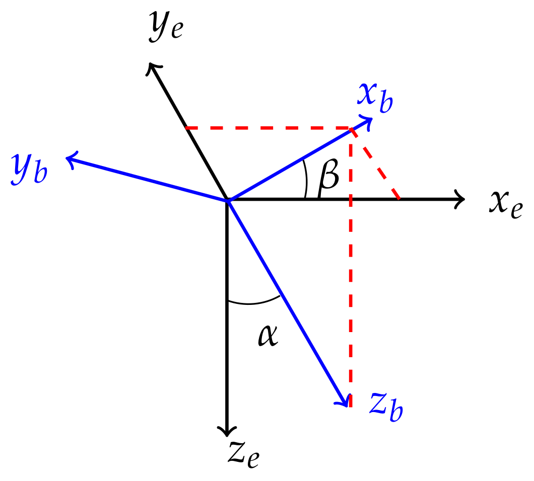
In our model problem, we consider two different Cartesian coordinate systems: (a) a system of coordinates related to the Earth, and (b) a system of coordinates related to the logging device, which consists of a rotation of the Earth system of coordinates in a way that the logging device extends along the z direction. We denote the angle between the logging instrument and the z direction of the Earth system of coordinates as $\alpha$ (relative dip angle). $\beta$ is the azimuthal angle (see Figure 5). Therefore, the transformation between the systems of coordinates of the Earth and the tool is given by the following rotation matrix:

$${\mathcal{H}}_b={\mathbf{R}}^{-1}{\mathcal{H}}_e\mathbf{R},$$

(85)

where rotation $\mathbf{R}$ is defined by the following composition of rotations:

$$\mathbf{R}=\left[\begin{array}{ccc}\cos \beta & -\sin \beta & 0\\ \sin \beta & \cos \beta & 0\\ 0& 0& 1\end{array}\right]·\left[\begin{array}{ccc}\cos \alpha & 0& \sin \alpha \\ 0& 1& 0\\ -\sin \alpha & 0& \cos \alpha \end{array}\right].$$

In this notation, subscripts e and b denote the Earth system of coordinates and the logging instrument system of coordinates, respectively. If the logging instrument is perpendicular to the layering of the medium, we have $\alpha =0$.

In this work, for simplicity, we consider $\beta =0$. Hence, the possibly non-zero couplings of the magnetic field can only be $xx$, $xz$, $yy$, $zx$ and $zz$, where the first and the second letters in the subscript indicate the transmitter and receiver directions, respectively.

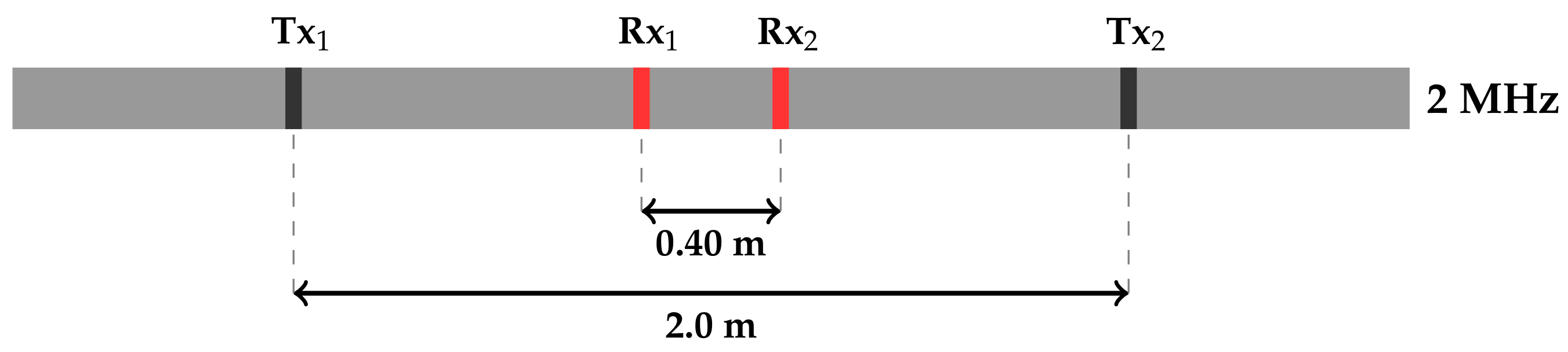
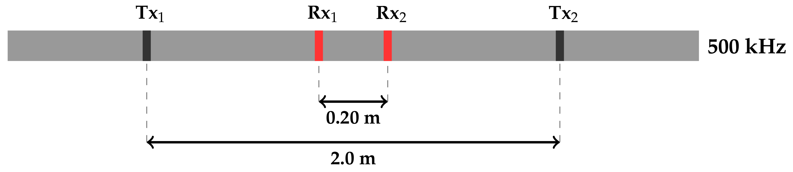
In this work, we consider LWD tools equipped with magnetic dipoles sources. We consider a traditional symmetric LWD instrument, which is a standard tool similar to those offered by oil service companies containing two transmitters and two receivers. In the aforementioned instrument, the receivers are located symmetrically around the transmitters (see Figure 6 and Figure 10) [22].

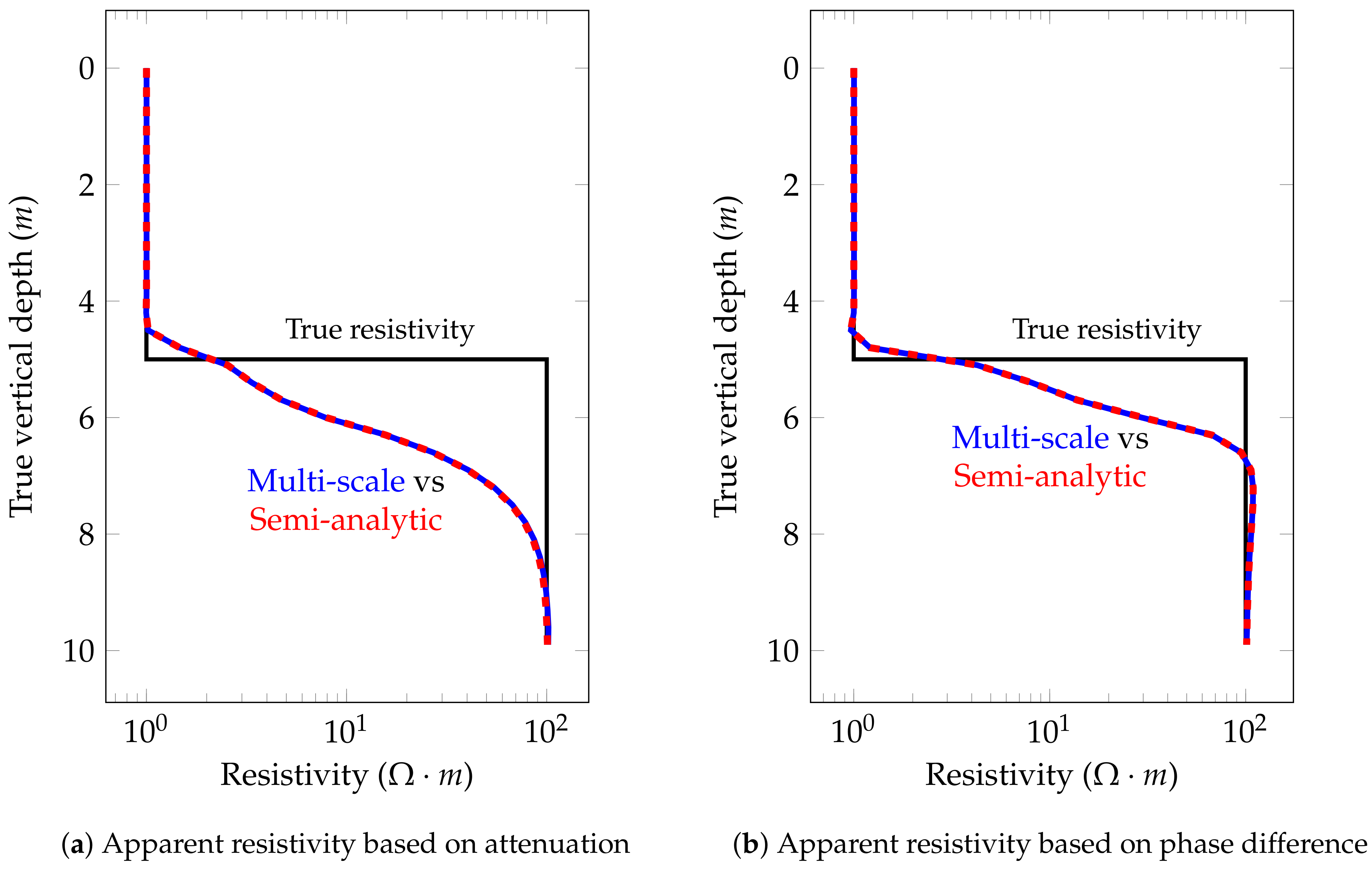
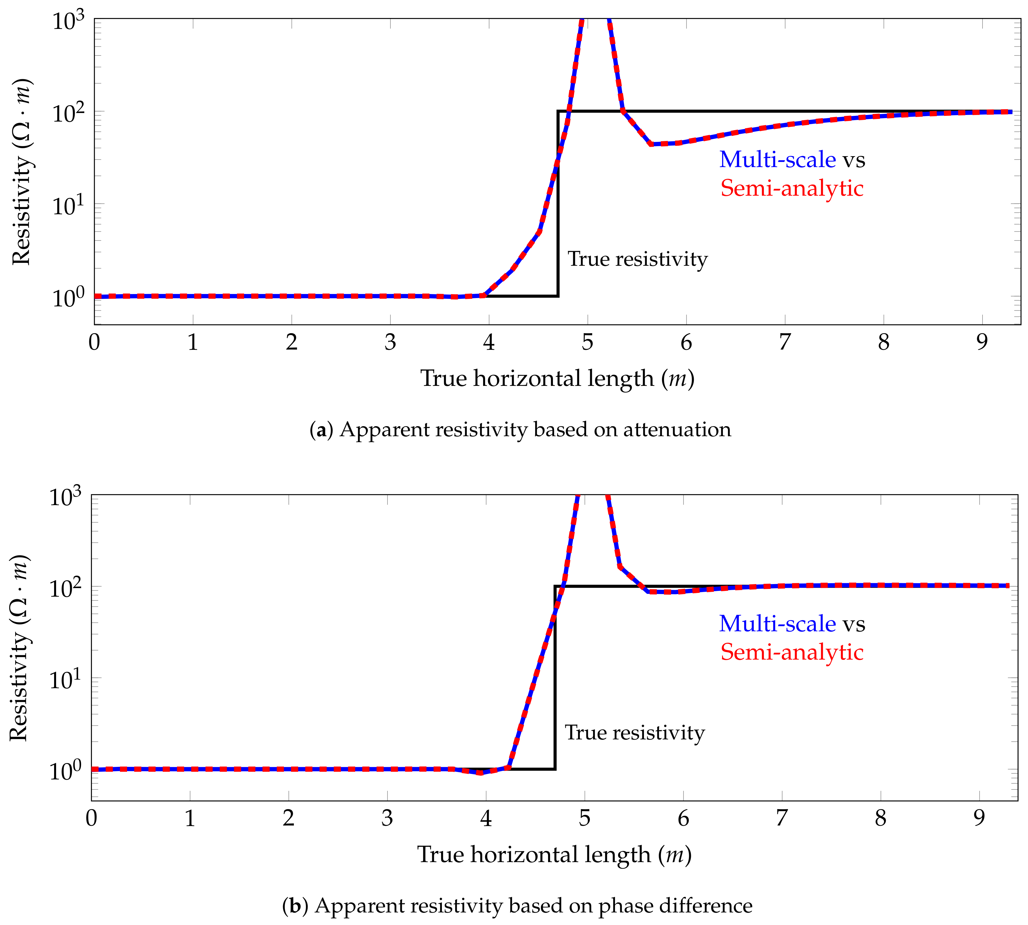
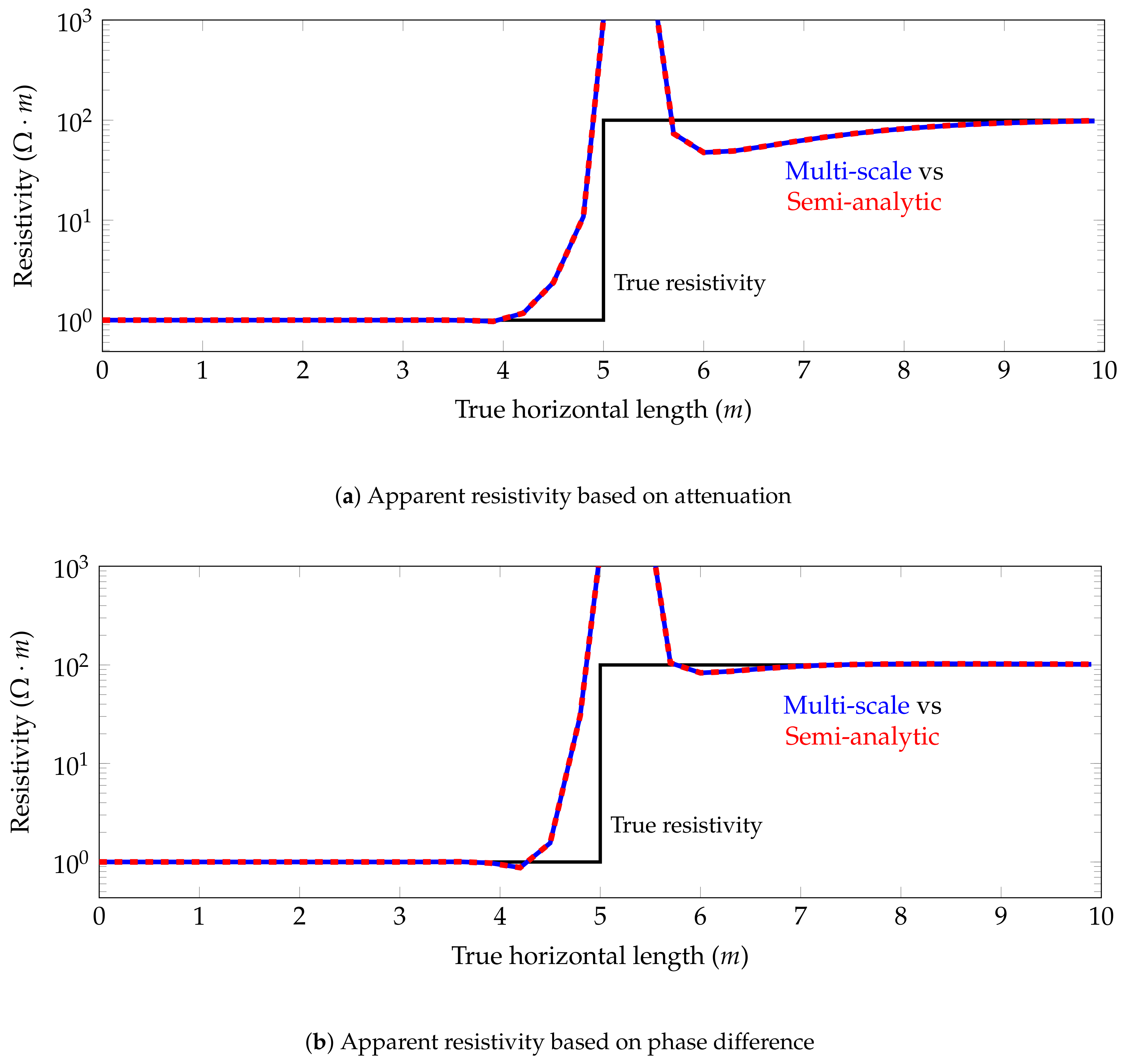
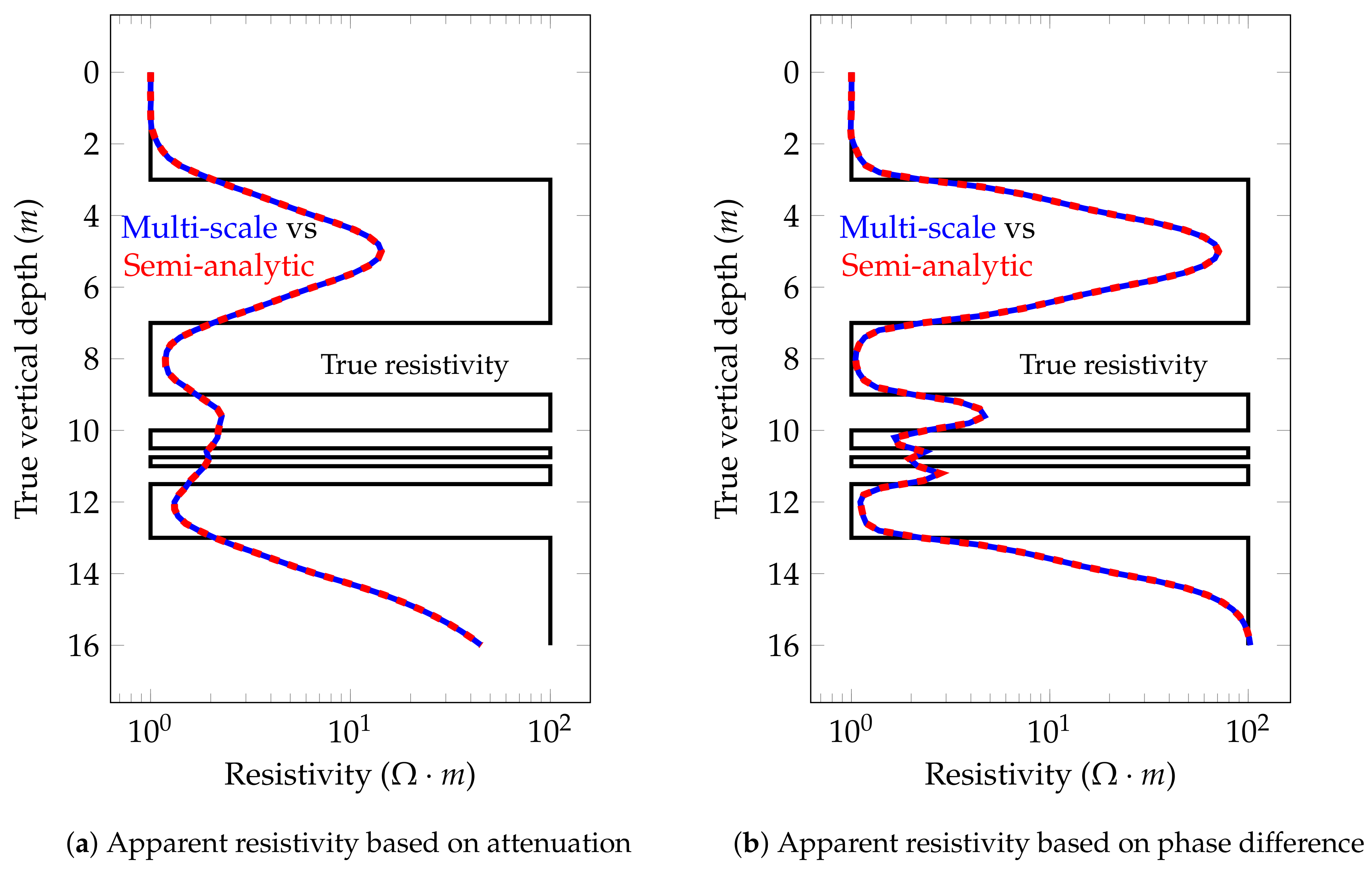
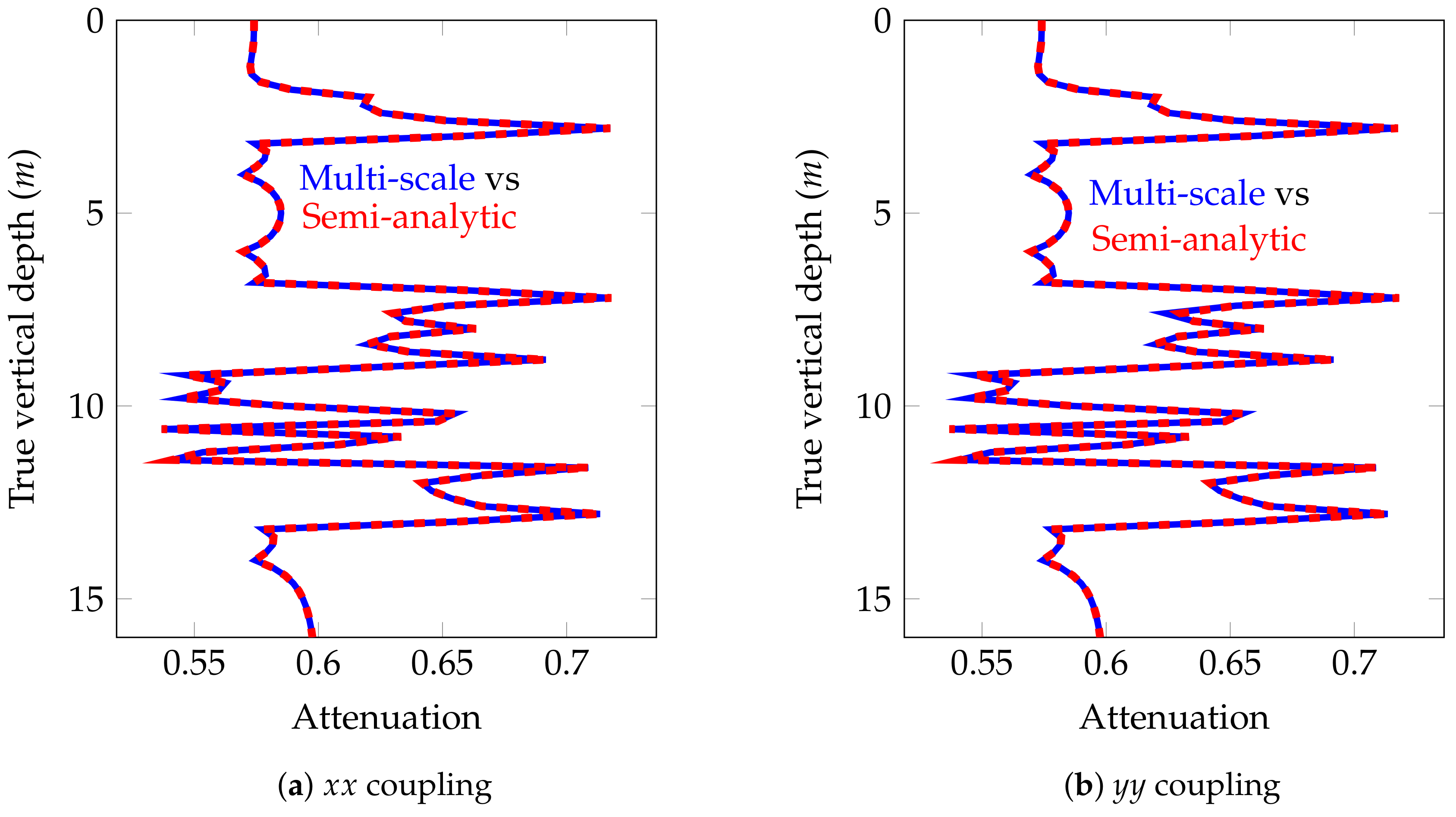
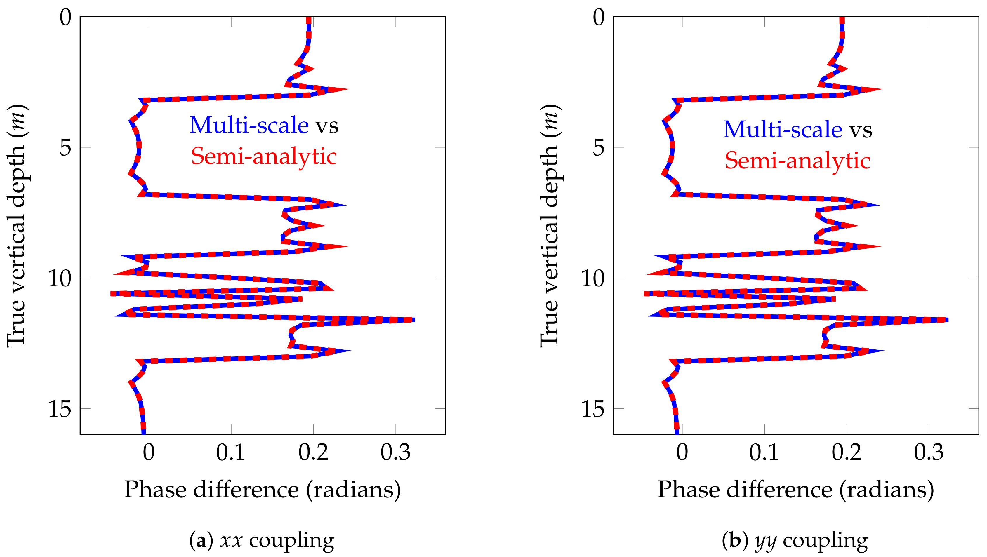
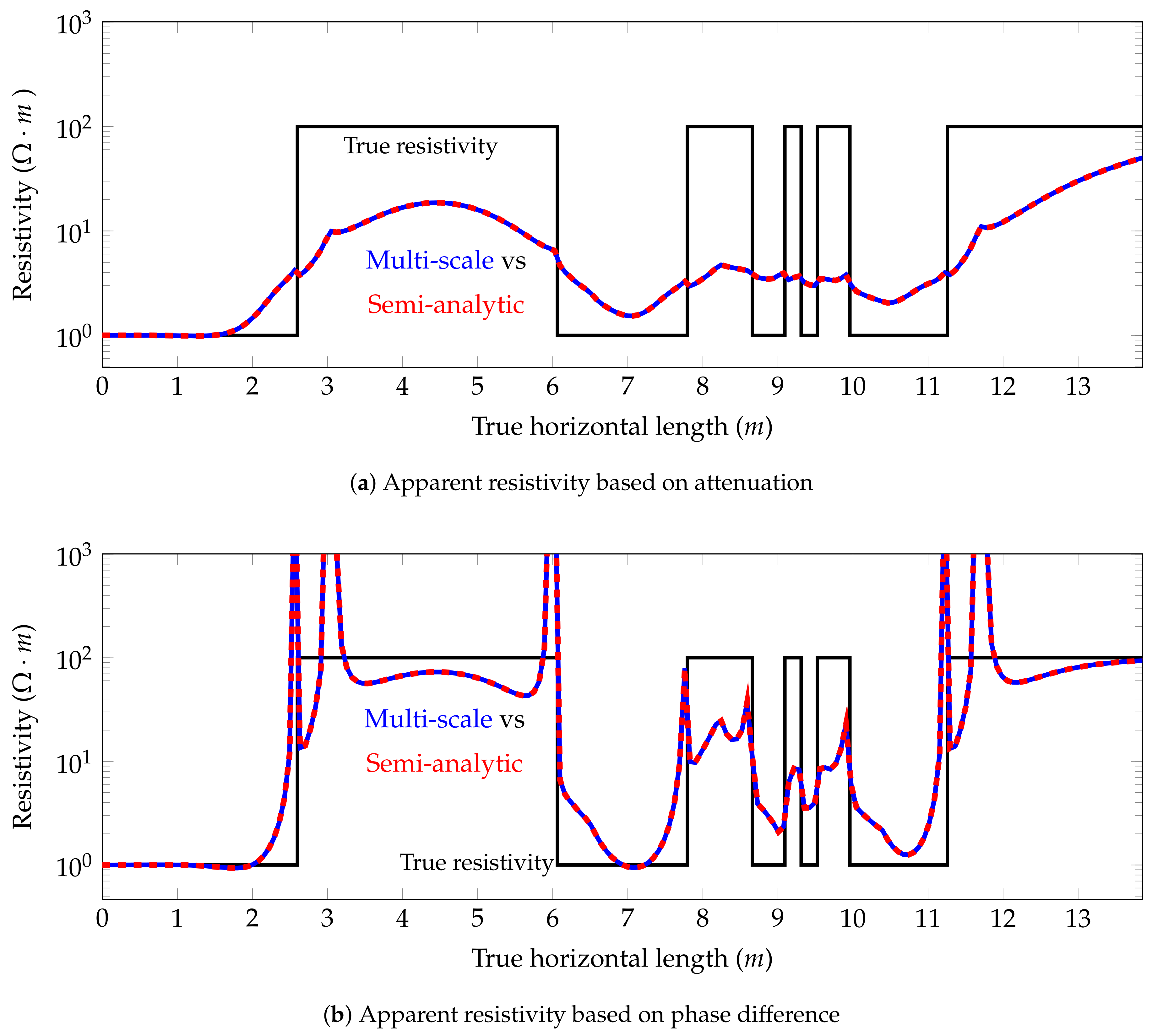
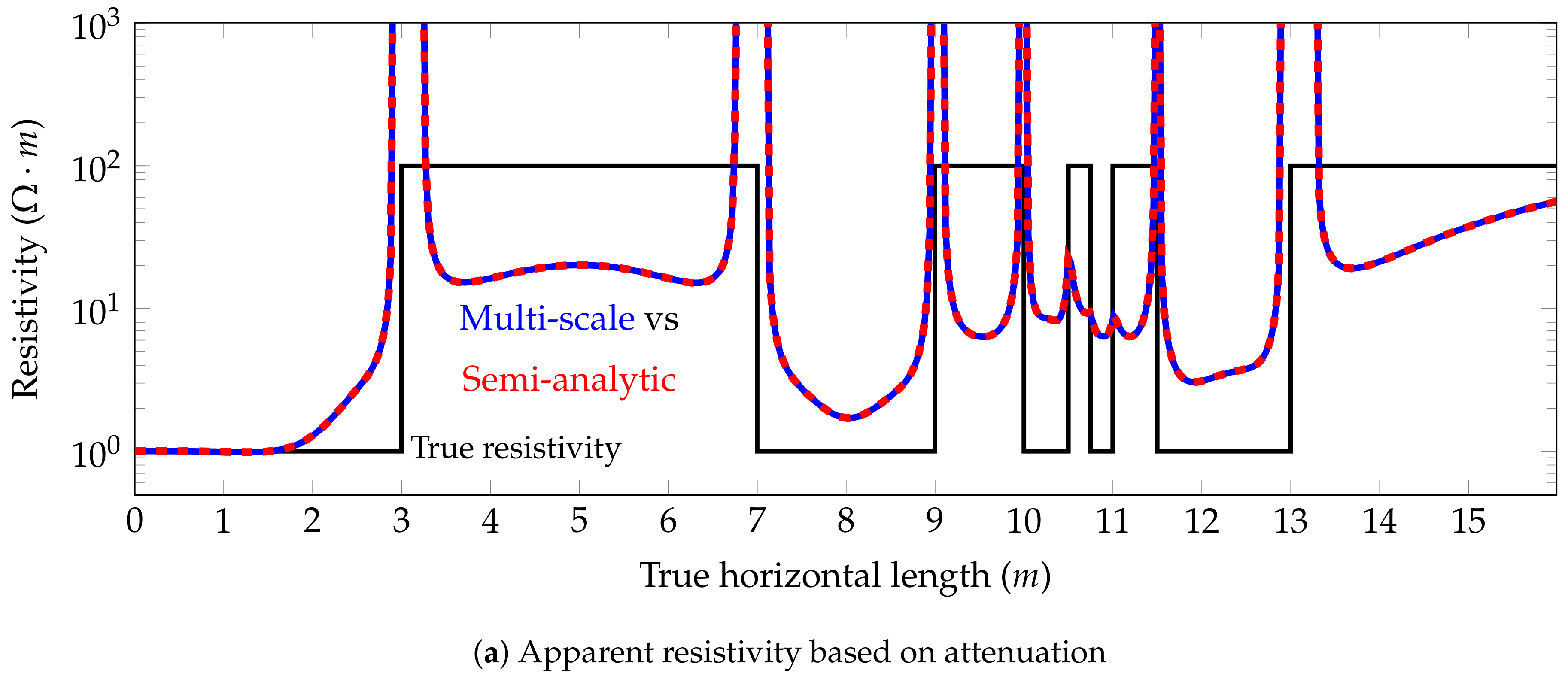
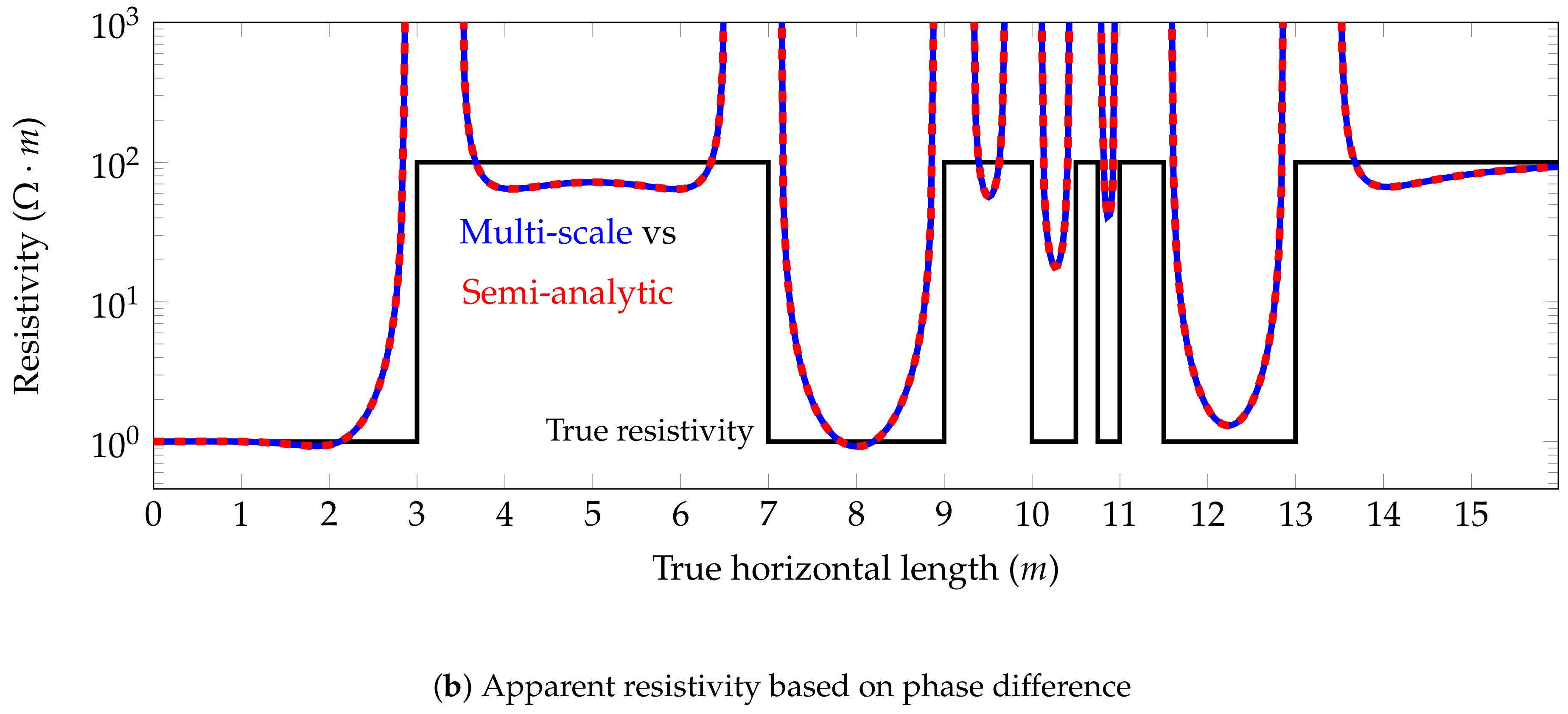
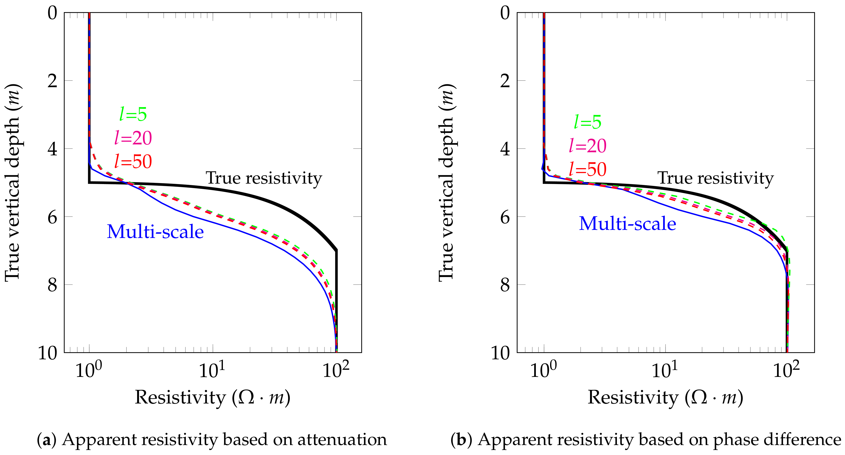
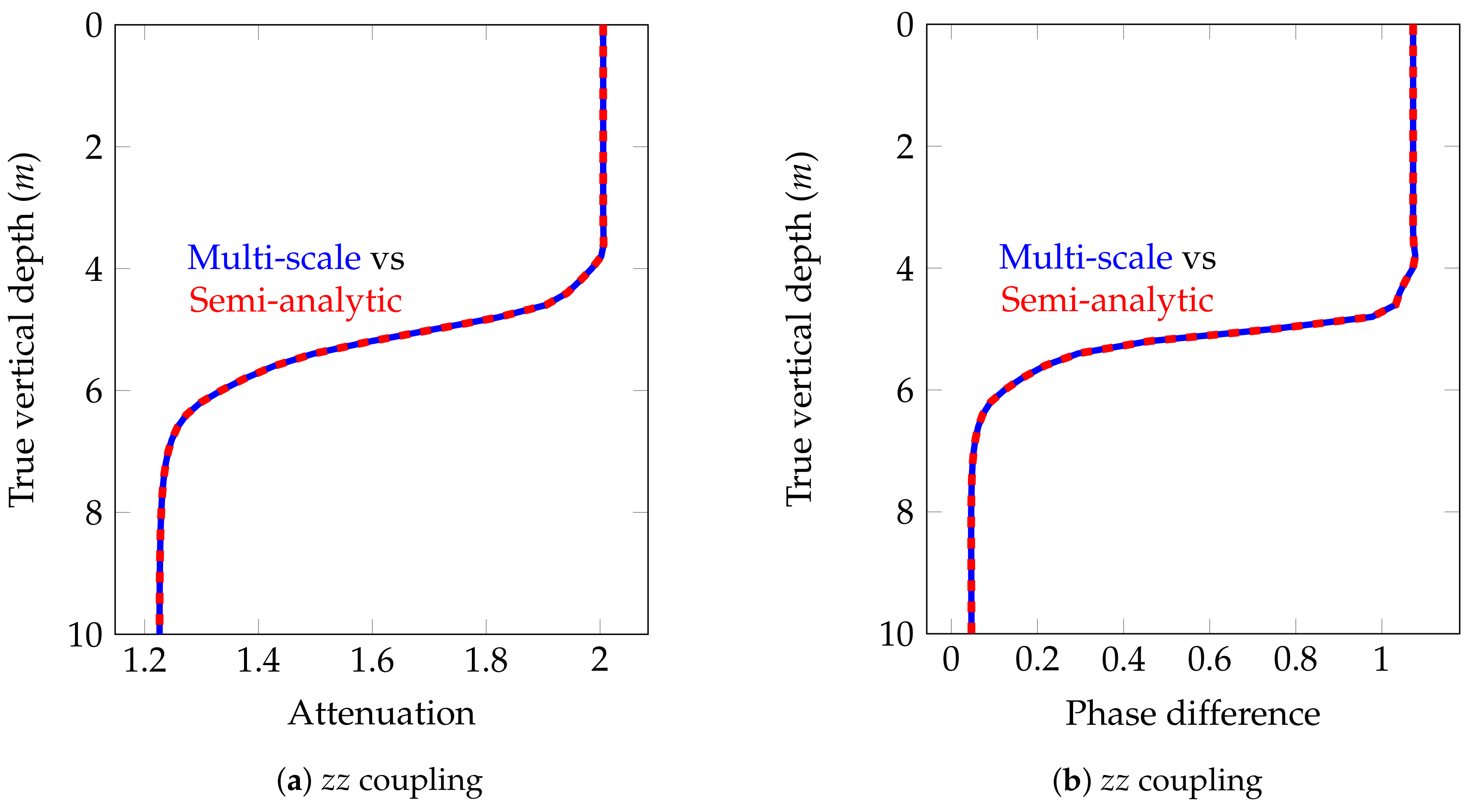
To analyze the result of our experiments and compare them against those typically obtained in borehole resistivity applications, we further postprocess the values of the magnetic field. First, we evaluate the $zz$ coupling (${\mathcal{H}}_{zz}$) of the magnetic field at two different receivers. We denote these values as ${\mathcal{H}}_{zz}\left(R{x}_1\right)$ and ${\mathcal{H}}_{zz}\left(R{x}_2\right)$, which correspond to the first and the second receiver, respectively. Then, we compute:

$$\ln \frac{{\mathcal{H}}_{zz}\left(R{x}_1\right)}{{\mathcal{H}}_{zz}\left(R{x}_2\right)}=\underset{\mathrm{attenuation}}{\underbrace{\ln \frac{\mid {\mathcal{H}}_{zz}\left(R{x}_1\right)\mid }{\mid {\mathcal{H}}_{zz}\left(R{x}_2\right)\mid }}}+i\underset{\mathrm{phase}\mathrm{difference}}{\underbrace{\left(ph\left({\mathcal{H}}_{zz}\left(R{x}_1\right)\right)-ph\left({\mathcal{H}}_{zz}\left(R{x}_2\right)\right)\right)}},$$

(86)

where $ph$ denotes the phase of a complex number. Often, the attenuation is defined in the decibel scale (which corresponds to the above number multiplied by 20). Subsequently, we compute the relation between attenuation and resistivity in a homogeneous media. This transformation, when applied to a heterogeneous media, delivers the apparent resistivity based on attenuation (see [5]). We similarly define the apparent resistivity based on the phase difference.

For the inverse Hankel transform, we use a fast Hankel transform algorithm based on digital filters (see [19] for details).

The entire Hankel Finite Element method has been implemented using FORTRAN 90.

6. Numerical Examples

6.1. Model Problem 1: Two Layers with 1 $\Omega ·m$ and 100 $\Omega ·m$

We consider the logging instrument described in Figure 6. Figure 7 through Figure 9 show the apparent resistivities (logs) for different dip angles. The distance between two consecutive logging points is half a foot (0.1524 m), as this is the resolution provided by most commercial logging-while-drilling (LWD) devices. In all cases, our simulation framework delivers a perfect agreement with the semi-analytic solutions. The large apparent resistivity values observed in Figure 8 and Figure 9 form the so-called horns. They are a typical artifact that appears due to the employed post-processing method [10,16]. Moreover, they do not affect significantly to the interpretation of the results.

6.2. Model Problem 2: Multilayered Formation

Figure 10 describes the logging instrument employed for this example. As in our previous examples, the distance between two consecutive logging points is half a foot (0.1524 m). The main result in terms of apparent resistivities for this model problem for a vertical well is shown in Figure 11. The attenuations and phase differences for this case are shown in Figure 12 and Figure 13, respectively. As before, the numerical solutions coincide with the semi-analytic ones.

Figure 14 compares the average computational time needed to solve one tool position using: (a) a traditional FE method, (b) a traditional FE method when we reuse the LU factorization, and (c) our proposed multi-scale method. As shown in the figure, reusing the LU factorization worsens the situation since we need a more refined grid to model for all source positions accurately.

Table 1. A time comparison (in seconds) for a vertical well using a semi-analytic method and the proposed multi-scale FEM as a function of the number of tool positions.

Positions	Semi-Analytic	Numerical	Ratio
1	$3.2\times {10}^{-2}$	5.67	177.19
10	$5.3\times {10}^{-2}$	12.34	232.83
100	$1.4\times {10}^{-1}$	15.60	111.43
200	$2.4\times {10}^{-1}$	18.73	76.54
500	$4.1\times {10}^{-1}$	23.10	56.34
1000	$1.01$	35.52	35.16
5000	$5.68$	115.47	20.65
10,000	$11.57$	207.61	17.94

shows a time comparison between a semi-analytic method and the proposed numerical method. For one tool position, computing the local primary field and pre-computing the multi-scale basis functions is computationally expensive and we observe a significant discrepancy between numerical and semi-analytic solutions. However, as expected, by increasing the number of tool positions, the ratio between the time of the proposed numerical method and the semi-analytic one is decreasing. Figure 15 shows the average time used to solve one tool position. Using a multi-scale method, the average time per position rapidly decreases as we augment the total number of tool positions. This occurs because the pre-computed multi-scale basis functions, fundamental fields, and correction basis functions only need to be computed once for any number of tool positions.

The results in terms of apparent resistivities for this model problem for ${60}^{\circ }$ and ${89}^{\circ }$ deviated wells are shown in Figure 16 and Figure 17, respectively. Again, the numerical and semi-analytic solutions coincide.

6.3. Model Problem 3: Non-Piecewise-Constant Resistivity Distribution

We consider the logging instrument described in Figure 6 and a model problem that exhibits a sub-domain with a linearly varying resistivity, which is the case of an oil-to-water saturated transitioning (OWT) zone corresponding to a two phase-flow of immiscible fluids. To compare our solution to the semi-analytic one in the later case, we approximate our linearly varying resistivity distribution using multiple piecewise constant resistivity distributions. Figure 18 shows that the apparent resistivity of the semi-analytic solution is converging to the multi-scale solution as the number of layers with piecewise constant resistivity distribution increases. With our numerical method, we can model those arbitrarily varying conductivities without the need of approximating them. Figure 19 compares the attenuation and phase difference of the ultimate semi-analytic solution and the multi-scale one for the $zz$ coupling.

7. Discussion and Conclusions

We propose a multi-scale Hankel FEM for solving Maxwell’s equations in a 1D Transversely Isotropic media excited by a 3D arbitrarily oriented point dipole. The multi-scale FEM pre-computes the fundamental fields, and correction and multi-scale basis functions. As a result, this computation is expensive if only a single logging position is studied, but it becomes competitive as the number of logging position grows.

The numerical method produces highly accurate solutions, as our numerical validations experiments show. Additionally, computation of the parametrization derivatives is straightforward by simply considering the adjoint formulation. By using this method, it is possible to consider arbitrary resistivity distributions along the z direction, while semi-analytic methods only allow for piecewise constant material coefficients.

The method we propose is still slower than the semi-analytic one. The most time consuming part of our method is to compute the primary field. However, in the case of piecewise constant resistivity distribution, we can obtain the fundamental field analytically, which decreases the cost of computing the primary field considerably. Nonetheless, this work employs a full FEM implementation to preserve the generality of the method. This enables us to consider arbitrary resistivity distributions (other than just piecewise constant ones). Because of the lack of existence of a semi-analytic method that can model the aforementioned case, our methodology is a viable alternative. In order to use a semi-analytic method, we can approximate the non-constant resistivity distribution using multiple constant resistivity distributions. However, this piecewise-constant representation leads to an extensive error and a bothersome implementation when computing the derivatives to form the Jacobian matrix to perform the inversion.

As future work, we plan to extend our method to other multi-physics problems e.g. elasto-acoustic problems and to account for other material parameter distributions, such as, cross-bedded formations. Also, we will investigate the optimal selection of the primary field. Moreover, we shall also integrate this simulator on an inversion software platform. A trivial parallelization of this software through operating frequencies and transmitters of a logging device and logging positions is straightforward. Additionally, the parallelization of the method through multi-scale basis functions, fundamental fields, and correction basis functions is under development, which will boost the speed of the method.

References

1. Bakr, S.A.; Pardo, D.; Mannseth, T. Domain decomposition Fourier FE method for the simulation of 3D marine CSEM measurements. J. Comput. Phys. 2013, 255, 456–470. [Google Scholar] [CrossRef]
2. Bakr, S.A.; Pardo, D. A multi-domain decomposition-based Fourier finite element method for the simulation of 3D marine CSEM measurements. Comput. Geosci. 2017, 21, 345–357. [Google Scholar] [CrossRef] [Green Version]
3. Puzyrev, V.; Koldan, J.; de la Puente, J.; Houzeaux, G.; V<i>a</i>´zquez, M.; Cela, J.M. A parallel finite-element method for three-dimensional controlled-source electromagnetic forward modelling. Geophys. J. Int. 2013, 193, 678–693. [Google Scholar] [CrossRef] [Green Version]
4. Alvarez-Aramberri, J.; Pardo, D. Dimensionally adaptive hp-finite element simulation and inversion of 2D magnetotelluric measurements. J. Comput. Sci. 2017, 18, 95–105. [Google Scholar] [CrossRef]
5. Pardo, D.; Torres-Verdin, C. Fast 1D inversion of logging-while-drilling resistivity measurements for the improved estimation of formation resistivity in high-angle and horizontal wells. Geophysics 2014, 80, E111–E124. [Google Scholar] [CrossRef]
6. Omeragic, D.; Habashy, T.; Chen, Y.H.; Polyakov, V.; Kuo, C.; Altman, R.; Hupp, D.; Maeso, C. Reservoir characterization and well placement in complex scenarios using LWD directional EM measurements. Petrophysics 2009, 50, 396–415. [Google Scholar]
7. Al-Musharfi, N.M.; Bansal, R.; Ahmed, M.S.; Kanj, M.Y.; Morys, M.; Conrad, C.; Parker, T.J. Real time reservoir characterization and geosteering using advanced high-resolution LWD resistivity imaging. In Proceedings of the SPE Annual Technical Conference and Exhibition, Florence, Italy, 19–22 September 2010; Society of Petroleum Engineers: Richardson, TX, USA, 2010; pp. 1–11. [Google Scholar]
8. Beer, R.; Dias, L.C.T.; da Cunha, A.M.V.; Coutinho, M.R.; Schmitt, G.H.; Seydoux, J.; Guedes, A.B.F. Geosteering and/or reservoir characterization the prowess of new-generation LWD tools. In Proceedings of the SPWLA 51st Annual Logging Symposium, Perth, Australia, 19–23 June 2010; Society of Petrophysicists and Well-Log Analysts: Houston, TX, USA, 2010; pp. 1–14. [Google Scholar]
9. Li, H.; Shen, Y.; Zhu, X. Numerical simulation of resistivity LWD tool based on higher-order vector finite element. J. Pet. Explor. Prod. Technol. 2016, 6, 533–543. [Google Scholar]
10. Zhang, C.; Wu, Q.; Wang, X.; Lu, N. Application of rotary geosteering drilling in deep and thin reservoirs of Tarim Basin, NW China. Pet. Explor. Dev. 2013, 40, 801–805. [Google Scholar] [CrossRef]
11. Kok, J.C.L.; DeJarnett, J.; Geary, D.; Vauter, E. Successful geosteering in low resistivity contrast reservoirs of the Permian Basin. In Proceedings of the SPE Eastern Regional Meeting, Columbus, OH, USA, 17–19 August 2011; Society of Petroleum Engineers: Richardson, TX, USA, 2011; pp. 1–4. [Google Scholar]
12. Erdozain, A.; Barucq, H.; Pardo, D.; Péron, V. Fast Inversion of 3D Borehole Resistivity Measurements Using Model Reduction Techniques Based on 1D Semi-Analytical Solutions. Ph.D. Thesis, Université de Pau et des Pays de l’Adour, Universidad del País Vasco-Euskal Herriko Unibertsitatea, Leioa, Spain, 2016. [Google Scholar]
13. Wang, G.L.; Barber, T.; Wu, P.; Allen, D.; Abubakar, A. Triaxial induction tool response in dipping and crossbedded formations. In SEG Technical Program Expanded Abstracts 2014; Society of Exploration Geophysicists: Tulsa, OK, USA, 2014; pp. 585–590. [Google Scholar]
14. Davydycheva, S.; Homan, D.; Minerbo, G. Triaxial induction tool with electrode sleeve: FD modeling in 3D geometries. J. Appl. Geophys. 2004, 67, 98–108. [Google Scholar] [CrossRef]
15. Loseth, L.O.; Ursin, B. Electromagnetic fields in planarly layered anisotropic media. Geophys. J. Int. 2007, 170, F44–F80. [Google Scholar] [CrossRef]
16. Davydycheva, S.; Wang, T. A fast modelling method to solve Maxwell’s equations in 1D layered biaxial anisotropic medium. Geophysics 2011, 76, F293–F302. [Google Scholar] [CrossRef]
17. Rojas, S.; Muga, I.; Pardo, D. A quadrature-free method for simulation and inversion of 1.5D direct current (DC) borehole measurements. Comput. Geosci. 2016, 20, 1301–1318. [Google Scholar] [CrossRef]
18. Lehe, R.; Kirchen, M.; Andriyash, I.A.; Godfrey, B.B.; Vay, J.L. Quasi-cylindrical and dispersion-free particle- In-Cell algorithm. Comput. Phys. Commun. 2013, 203, 66–82. [Google Scholar] [CrossRef]
19. Key, K. Is the fast Hankel transform faster than quadrature? Comput. Phys. Commun. 2012, 77, F21–F30. [Google Scholar] [CrossRef]
20. Muga, I.; Ossandón, S. A method to compute the surface Green’s function of piezoelectric half-space. Scientia 2006, 13, 84–91. [Google Scholar]
21. Demkowicz, L. Encyclopedia of Computational Mechanics. In Finite Element Methods for Maxwell’s Equations; Oxford University Press: Oxford, UK, 2004; pp. 1–26. [Google Scholar]
22. Liu, H. Principles and Applications of Well Logging; Springer: Berlin, Germany, 2017. [Google Scholar]
23. Nédélec, J.-C. Acoustic and Electromagnetic Equations; Springer: Berlin, Germany, 2001. [Google Scholar]
24. Ward, S.H.; Hohmann, G.W. Electromagnetic Methods in Applied Geophysics: Volume 1, Theory; Society of Exploration Geophysicists: Tulsa, OK, USA, 1987. [Google Scholar]
25. Kong, J.A. Electromagnetic Wave Theory; Wiley-Interscience: Hoboken, NJ, USA, 1986. [Google Scholar]
26. Kirscha, A.; Hettlich, F. The Mathematical Theory of Time-harmonic Maxwell’s Equations; Springer: Berlin, Germany, 2015. [Google Scholar]
27. Abramowitz, M.; Stegun, I.A. Handbook of Mathematical Functions with Formulas, Graphs and Mathematical Tables; National Bureau of Standard: Washington, DC, USA, 1964. [Google Scholar]
Figure 1. Cartesian and cylindrical systems of coordinates.
Geosciences 08 00225 g001
Figure 2. Selected decomposition points z 1 , , z N - 1 in the domain ( z 0 , z N ) . Ω 1 , Ω 2 , , Ω N are the sub-domains associated to the decomposition points.
Geosciences 08 00225 g002
Figure 3. Multi-scale basis functions ψ 1 , 1 , ψ 2 , 1 , , ψ N - 1 , 1 and local primary field H P . Ω p is the domain of the local primary field.
Geosciences 08 00225 g003
Figure 4. Fundamental, correction and local primary fields.
Geosciences 08 00225 g004
Figure 5. x e , y e and z e are the axes of the Cartesian coordinates. x b , y b and z b are the axes of the borehole coordinates. α and β are the dip and azimuthal angles, respectively.
Geosciences 08 00225 g005
Figure 6. Logging instrument for model problem 1. Tx 1 and Tx 2 are the induction transmitters, and Rx 1 and Rx 2 are the receivers.
Geosciences 08 00225 g006
Figure 7. Model problem 1. Apparent resistivities for the z z coupling for a vertical well (dip angle = 0 ).
Geosciences 08 00225 g007
Figure 8. Model problem 1. Apparent resistivity for the z z coupling for a 70 deviated well.
Geosciences 08 00225 g008
Figure 9. Model problem 1. Apparent resistivity for the z z coupling for a 89 deviated well.
Geosciences 08 00225 g009
Figure 10. Logging instrument for model problem 2. Tx 1 and Tx 2 are the induction transmitters, and Rx 1 and Rx 2 are the receivers.
Geosciences 08 00225 g010
Figure 11. Model problem 2. Apparent resistivity for the z z coupling for a vertical well (dip angle = 0 ).
Geosciences 08 00225 g011
Figure 12. Model problem 2. Attenuations for the non-zero couplings ( x x and y y couplings) of the magnetic field for a vertical well (dip angle = 0 ).
Geosciences 08 00225 g012
Figure 13. Model problem 2. Phase differences for the non-zero couplings ( x x and y y couplings) of the magnetic field for a vertical well (dip angle = 0 ).
Geosciences 08 00225 g013
Figure 14. Model problem 2. Average time (in seconds) to solve for one tool position as the number of logging positions varies using (a) a traditional FE approach, (b) a FE approach where we reuse the LU factorization, and (c) our proposed multi-scale method ( time ( seconds ) number of tool positions ).
Geosciences 08 00225 g014
Figure 15. Model problem 2. Average time (in seconds) to solve for one tool position as the number of tool positions varies ( time ( seconds ) number of tool positions ).
Geosciences 08 00225 g015
Figure 16. Model problem 2. Apparent resistivity for the z z coupling for a 60 deviated well.
Geosciences 08 00225 g016
Figure 17. Model problem 2. Apparent resistivity for the z z coupling for a 89 deviated well.
Geosciences 08 00225 g017aGeosciences 08 00225 g017b
Figure 18. Model problem 3. Convergence of the z z coupling apparent resistivity of the semi-analytic solution to the multi-scale one for a vertical well (dip angle = 0 ). l is the number of piecewise constant resistivity distributions that we select to approximate the linearly varying resistivity.
Geosciences 08 00225 g018
Figure 19. Model problem 3. Attenuation and Phase difference of the magnetic field for a vertical well (dip angle = 0 ).
Geosciences 08 00225 g019