Article

Geophysical Input to Improve the Conceptual Model of the Hydrogeological Framework of a Coastal Karstic Aquifer: Uley South Basin, South Australia

1
South Australian Water Corporation, 250 Victoria Square, Adelaide, SA 5000, Australia
2
Zonge Engineering and Research Organization (Australia) Pty Ltd., 39 Raglan Avenue, Edwardstown, SA 5039, Australia
*
Author to whom correspondence should be addressed.
Geosciences 2018, 8(7), 226; https://doi.org/10.3390/geosciences8070226
Submission received: 17 May 2018 / Revised: 19 June 2018 / Accepted: 19 June 2018 / Published: 21 June 2018

Abstract

:
A lack of closely spaced datasets on layer elevations, aquifer parameters, identification of areas with high recharge potential, dominant conduit porosity zones, and well defined boundary conditions hampers the ability of groundwater models to produce a reliable water balance. Typically, geological structure, aquifer properties, and groundwater heads are obtained from point measurements which are sparse. The drillhole information in aquifers is usually available at locations far apart, distances ranging from hundreds to thousands of meters. Furthermore, pump tests are usually conducted at limited locations and generalized to the aquifer. This limited knowledge leads to errors in the conceptual understanding of the aquifer. In this study, Airborne Electromagnetic Survey (AEM) was used to define base elevations of the aquifers where drillhole information was lacking. Surface Nuclear Magnetic Resonance (sNMR), borehole NMR, Transient Electromagnetic (TEM), and downhole geophysical surveys have given new insight to the conceptualization of hydrogeological framework. These methods are relatively low in cost compared to traditional well drilling and provide information on layer elevations, aquifer parameters, point and diffuse recharge zones, and conduit porosity zones in the profile, which improves our definition of the boundary conditions. From a practical point of view, combining drillhole information with a variety of geophysical techniques provides sound datasets to develop a comprehensive conceptual model. This in turn can be used to build a robust groundwater model.

1. Introduction

For effective groundwater management, reliable estimation of the water balance is a pre-requisite. Groundwater models are commonly developed to understand regional groundwater systems and guide the decisions on water resources management [1]. Groundwater models provide a scientific and predictive tool for determining appropriate solutions to water allocation, surface water–groundwater interaction, landscape management, or impact of new development scenarios. However, if modelling studies are not well designed from the outset, or the model doesn’t adequately represent the natural system being modelled, the modelling effort may be largely wasted, or decisions may be based on flawed model results, and long term adverse consequences may result [2]. In this context, it is considered that uncertainty in model results arise from errors in model structure, inputs, and parameters [3]. Rojas et al. [3] discussed this aspect further illustrating the fact that, typically, the geological structure is only partially known and point measurements of subsurface properties or groundwater heads are sparse and prone to error. Consequently, incomplete or biased process representation, errors in the specification of initial and boundary conditions, as well as errors in the model parameters, render the predictions of groundwater dynamics useless [3]. The importance of minimizing uncertainty in conceptual model has been widely recognized [4,5]. According to Ye et al. [6], uncertainties in geological interpretations can have larger effects on numerical model predictions than uncertainties in recharge estimates.
Thus, a critical step in the investigation of a groundwater flow system is the development of a conceptual model [7], where the hydrogeological framework is the most important. Typically, model parameter calibration methods are widely used in the hope for reducing uncertainty. Rojas et al. [3] highlight that despite its extensive application; the major weakness of parameter-calibration approaches is that all sources of uncertainty are attributed to parameter errors. This can result in biased parameter estimates that compensate for errors in model structure, input data, and measurement errors [3]. In groundwater systems, the conceptual model often includes: recharge sources, mechanism, and flux; groundwater flow direction, mechanism and paths; discharge locations, mechanism, and flux; hydrostratigraphy; vertical and horizontal aquifer boundary conditions; solute and isotopic evolution, and; steady or transient state conditions [7].
Karst aquifers are especially difficult to exploit, manage, and protect due to the extreme variability in their hydraulic properties, and presence of both diffuse and point recharge [8]. Karst aquifers possess both diffuse and conduit flow and varying degrees of connectivity between surface and groundwater over spatial scales [9]. Zhu et al. [10] state that locating conduit flow paths from the surface however, is one of the most challenging tasks in karst research. Geophysical methods are often used to help locate voids, by mapping variations of physical properties of the subsurface [10], as the conduits can cause significant contrasts in some physical properties that can be detected. Electrical resistivity is one of the commonly used geophysical methods for subsurface void detection, as a water-filled underground void has lower resistivity than most surrounding rocks; whereas an air filled void has higher resistivity than most geologic material [10]. An added advantage of using geophysical techniques is that they allow large areas to be covered in a short period of time and represent an efficient way of detecting subsurface heterogeneities including voids [11].
Several geophysical methods have been tested in the past to detect sinkholes and conduit flowpaths. They include conductivity mapping with the EM-31 and EM-34 methods [12] and electrical resistivity tomography using multi-array electrodes [13,14,15,16]. A study by Wedekind et al. [17] shows that surface geophysical data can be combined with downhole measurements to locate sinkholes more accurately. An important study was conducted by Jardani et al. [18], where the self-potential and electromagnetic (EM-34) method was used to reconstruct the geometry of the subsurface and to locate sinkholes. According to Jardani et al. [18], the self-potential method is the only geophysical method that is sensitive to the flow of groundwater, while the inversion of the EM data provides the distribution of electrical conductivity, which is sensitive to the water and clay contents of the subsurface. Sinkholes correspond to marked high conductivity depressions in the profile where the infiltrated water is channeled from unsaturated zone and percolates to the aquifer [18].
The primary objective of this study is to improve the existing conceptual model of the hydrogeological framework of the Uley South Basin, a coastal karstic aquifer. Previous conceptual understandings based on limited drillhole information of the Uley South Basin include: inter-aquifer leakage occurs only through two small reaches in northern boundary; the role of sinkholes and presence of point recharge has been considered as minor; presence of conduit flow zones in the basin has not been identified; aquifer parameters were known only at pump tested production wells and no knowledge about the range of parameter values in other parts of the basin; and the role of basement high areas on groundwater flow and boundary conditions not well defined. In recent years, 2015, 2016, and 2017, the basin has received low annual recharge of 49 mm, 84 mm, and 75 mm, respectively; well below the long term average annual recharge of 122 mm. In response to low recharge, groundwater levels have declined by 0.4–0.6 m over the three year periods. Currently, Uley South groundwater extraction is about 5 × 10⁶ m3 per year; however, concern has arisen regarding how long the current extraction could continue, and what is the optimum extraction rate under prolonged drought conditions. The need to improve existing knowledge is recognized, and to build a robust groundwater model for Uley South for testing a variety of management scenarios and ascertain the capacity of the basin under drought conditions.
The approach we followed was to utilize geophysical investigations with previous well drilling and pump testing over the 1940–2017 period, considered the major hydrogeological knowledge base. Of particular significance previous geophysical investigations were; the use of an Airborne Electromagnetic Survey (AEM) to map the extent and depth of aquifers [19]; and Nuclear Magnetic Resonance (NMR) survey to determine whether there is additional water in inaccessible sites for drilling, conductivity and drainable porosity of the aquifer [20]. In addition, Transient Electromagnetic (TEM) survey along selected transects across the basin, and downhole geophysical surveys of all monitoring wells were conducted in May, September–October 2017. Data were combined to produce the conceptual model of hydrogeological framework of the basin that provides the basis for constructing improved numerical models.

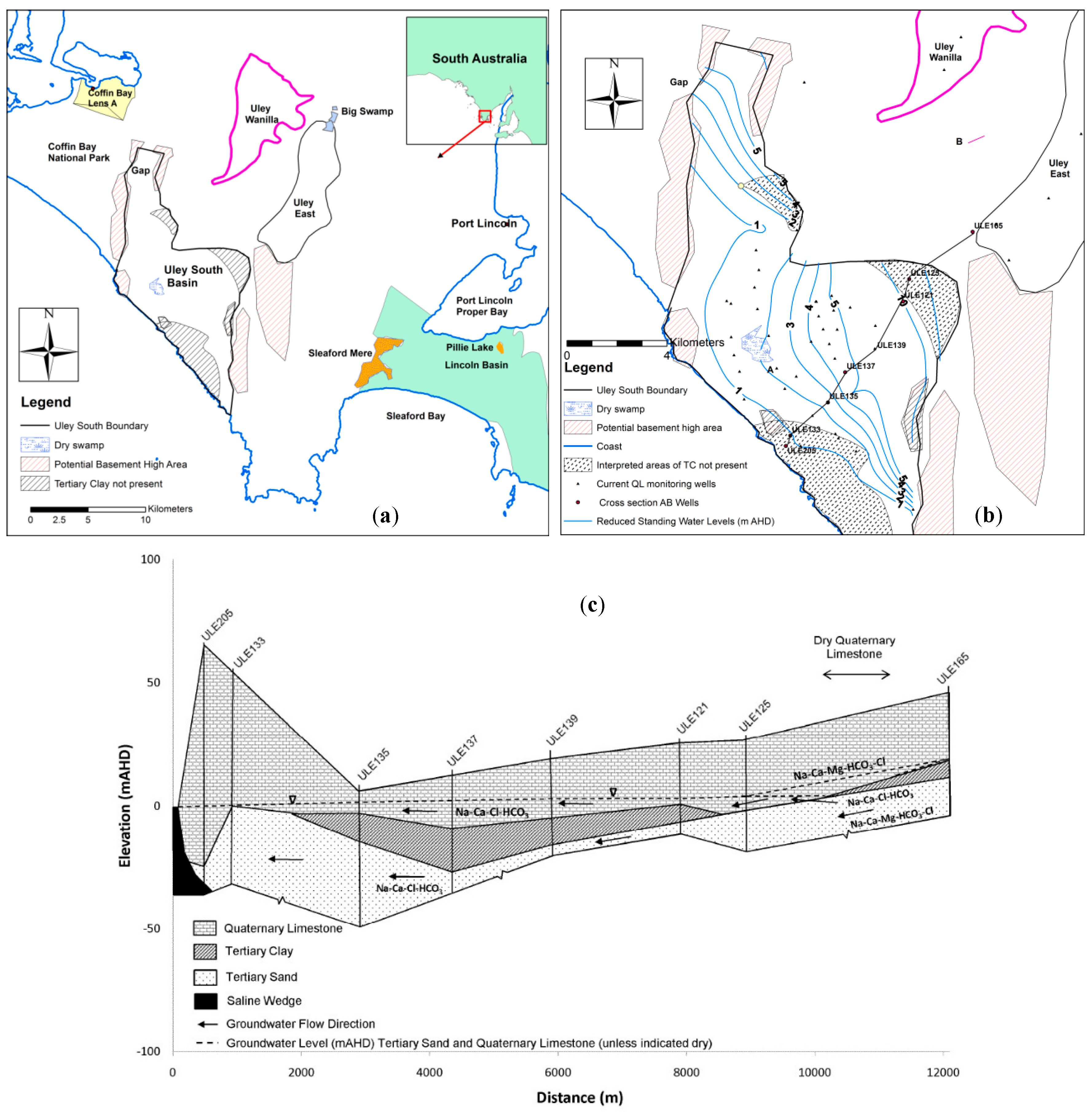
2. Geology and Hydrogeology of the Study Site

Groundwater provides 77% of the Eyre Peninsula (EP) water supply system from Southern basins (Uley South, Coffin Bay, Uley Wanilla, Uley East and Lincoln Basin) (Figure 1a). Of these groundwater supplies, the Uley South Basin is the largest and most strategic. The basin is located 22 km west of the city of Port Lincoln. The Uley South basin is approximately 113 km2 in area and is located on the Southern EP of South Australia (Figure 1a). The region has a semi-arid climate, which is characterized by winter-dominant (June–August) rainfall and hot, dry summer (December–February) [21]. Long-term average annual rainfall is 550 mm and average annual pan evaporation is 1550 mm. There is no well-developed soil horizon and the surface is composed mainly of skeletal soils: sandy or clayey loam, overlying calcrete [22]. The low lying central part of the basin contains numerous sinkholes. Runoff is highly ephemeral, occurring only after moderate to high intensity rainfall and persisting only tens to hundreds of meters before entering a vast array of epikarsts and sinkholes. A survey of a 4 km2 area found a density of about one sinkhole per 0.07 km2 with approximate size ranging from 0.4 to 2.5 m diameter [23].
The morphology of the basin is associated with ancient dune systems overlying basement ridges and troughs, with distinct dunal landforms and subtle undulations defining local surface drainage systems [21]. The hydrogeology of Uley South basin comprises Quaternary Limestone (QL) of an average thickness of 15–30 m, underlain by a Tertiary Clay (TC) unit of 5–25 m thickness, and a Tertiary Sand (TS) aquifer. The QL aquifer is highly heterogeneous, a typical feature of karstic aquifers. From pump testing carried out on production wells at 22 locations, hydraulic conductivity of the QL aquifer is found in the range of 131–2196 m·d−1, and specific yield ranges from 0.03–0.72. The TC is discontinuous and forms an aquitard between the TS and the QL aquifer systems. Uley South basin may be linked to the adjacent Coffin Bay aquifer through the basement low area (Gap in Figure 1a) in the north-western boundary. Groundwater flow direction is from north-east to south-west towards the coast (Figure 1b). The basement high area between Coffin Bay National Park and Uley South restricts groundwater movement to the west, except potential basement low area of 700 m (Gap in Figure 1a) [24]. Uley South QL aquifer receives recharge from three sources; diffuse recharge, point recharge from sinkholes and continuous leakage of TS water from the northern boundary where TC is absent [24] (Figure 1c). During intense rain events, runoff from neighboring limestone dry areas and basement high areas drains to karstic features in Uley South that recharge the aquifer (ibid). The basin is topographically closed and bounded by coastline and sand dunes to the west; and inland to the north and east by topographic rises of dry limestone.
The basin has been used for reticulated town water supply since 1976 and currently about 5 × 10⁶ m3 per year of groundwater is extracted from the Quaternary Limestone (QL) aquifer. Since 1977, the basin had received 532 × 106 m3 of rainfall recharge and the total groundwater extraction is about 306 × 106 m3 (57.5%) for the same period.

3. Materials and Methods

The traditional approach to define the hydrogeological framework is to use available drillhole information. In an area covering Uley South, Uley Wanilla, and Uley East groundwater basins (Figure 1a), lithological logs from drillholes were used to define aquifer/aquitard base elevations as the primary data source: having 221 data points for QL; 120 points for TC and 102 points for TS. However, there were large areas in Uley South and Coffin Bay where drillhole information was lacking. Therefore, one of the main aims of using AEM was to map elements of the Quaternary and Tertiary aquifer system in the Coffin Bay and Uley South area and the basement elevations [19]. The method and data analysis procedure is described in detail by Fitzpatrick et al. [19] and a brief summary is provided here. The survey was undertaken using the TEMPEST AEM system. The TEMPEST AEM system has a transmitter loop slung around a fixed wing aircraft and receiver coils in a towed bird. The TEMPEST system operates with a square transmitter waveform and fast sampling of received data combine to give very broad bandwidth, 25 to 37,500 Hz. In this respect, the system was considered particularly suited to the issue of defining the significant elements of the aquifer systems found on the lower EP. Comprehensive calibration procedures and advanced digital signal processing routines also ensure that accurate ground response information can be extracted from the measured TEMPEST data. The flight lines were orientated NW–SE with a nominal line spacing of 400 m [19].
The process of NMR data acquisition is described by Davis et al. [20] and the reader is directed to Davis et al. [20] for detail. Two sets of data acquisition, surface NMR (sNMR) and borehole NMR (bNMR), were used in the study area. The sNMR procedure included; a loop laid out at the site (typical loop side lengths are on the order of tens of metres to about 150 m, depending on the type of measurement wanted and the noise characteristics of the location); a transmitter attached to the loop, and the circuit was tuned to resonate at the Larmor frequency of the hydrogen nuclei at the site; a series of measurements were taken at the site with several different pulse lengths and pulse strengths of pumping current. The Uley South sNMR survey was conducted using the GMR multi-channel surface NMR equipment consists of a power source of two 12 V batteries connected in series to a 4000 V DC/DC converter. The sNMR loop size varied between a 145 m square loop and a 75 m square loop, depending on sounding depth required [20]. At each site, at least one noise cancellation loop was deployed [20]. Topographic information of sNMR sites are given relative to SRTM [26] elevations.
Borehole NMR logging was conducted similar to surface nuclear magnetic soundings, but there were some fundamental differences between them. In both cases, the nuclear magnetic resonance effect relies on a pulsed magnetic field that operates at right angles to the polarizing static magnetic field. In sNMR the static magnetic field is the magnetic field of the earth, while in borehole NMR, the static magnetic field is produced from powerful magnets that are mounted in the sonde and lowered down the borehole. The powerful magnets create a cylindrical shell of uniform field strength that is considered outside the invasion zone caused by the drilling technique [20].
The downhole geophysical logs were obtained using borehole logging unit of the South Australian Department of Environment and Water. The unit consists of data processing unit, winch, cable, and logging tools installed in a van. Gamma and neutron probes were run simultaneously. The surface unit controls the logging and movement of the probe and displays and stores data [15]. The probe is connected to the surface unit with the cable that conveys the electrical signals [27]. Downhole geophysical logging provides additional in-situ information to supplement the direct geological information. This is particularly useful where boreholes intercept small cavities which are unable to identify due to insufficient recovery of core samples or from observed minor lost-circulation [15]. Downhole geophysical logs provide continuous depth record of formation properties [27] such as: caliper logs provide information on drillhole diameter and fractures and are essential in interpreting other logs; gamma logs provide a record of natural radioactivity of the rock penetrated by a drillhole and provides information on lithology and stratigraphic correlation by relating to clays and silt content and permeability; neutron log measures neutrons from an isotopic source at one or several detectors after they migrate through material in, and adjacent to, the borehole.
The method of TEM and data interpretation was previously described by Somaratne and Mann [15]. For completeness, a summary is provided here. Seven high resolution TEM lines of varying orientation with station spacing of 25 m with infill to higher resolution (12.5 m) were used over areas of surface features such as sinkholes. A Zonge International GDP-32ii receiver equipped with NanoTEM cards were used to acquire all data for this study. Data were sensed using a single turn 5 m × 5 m wire loop placed at the centre of each transmitter loop. Data were recorded over two channels, with the second gained up to improve late time decay resolution. Decay data were recorded over 31 time windows to approximately 2 milliseconds after transmitter turnoff. Transmitted fields were generated with a Zonge NT-20 geophysical transmitter energizing a single turn 25 m × 25 m loop. This transmitter provides an output of 3 Amps, at 32 Hertz with a turn-off ramp time of 1.5 μs. Synchronisation was controlled directly using the GDP-32ii receiver. The receiver sampling interval used here is 1.6 μs which allows the system to be sensitive to geoelectric conditions very near surface. The NanoTEM system is battery powered and can be carried by hand which was important for applying this method in areas of thick scrub often encountered across the study area. Data were then used to produce 1D inversion model sections of resistivity using Zonge International’s STEMINV modelling program [15]. Ground elevations at bore locations are from surveyed elevations and in between SRTM [26] data were used. The sedimentary and largely flat lying geology encountered within the survey area offer ideal conditions for 1D modelling to provide accurate results. A true reflection of significant 2D and 3D features may be less well represented with this modelling approach however given the limited size of karst compared to the scale of the station spacing and loop size, these effects are expected to be minimal and not to compromise interpretability of the TEM models.

4. Results and Discussion

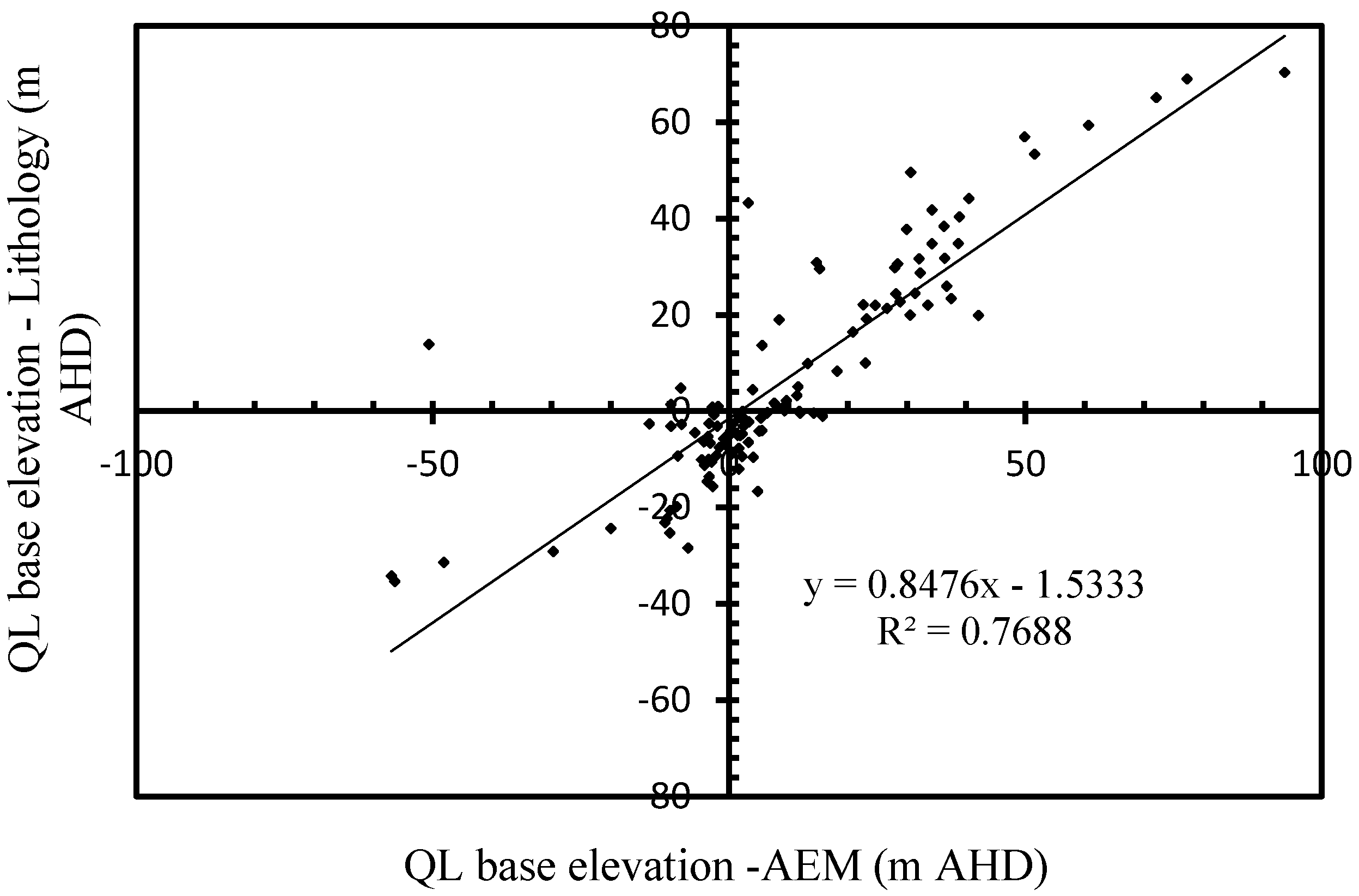
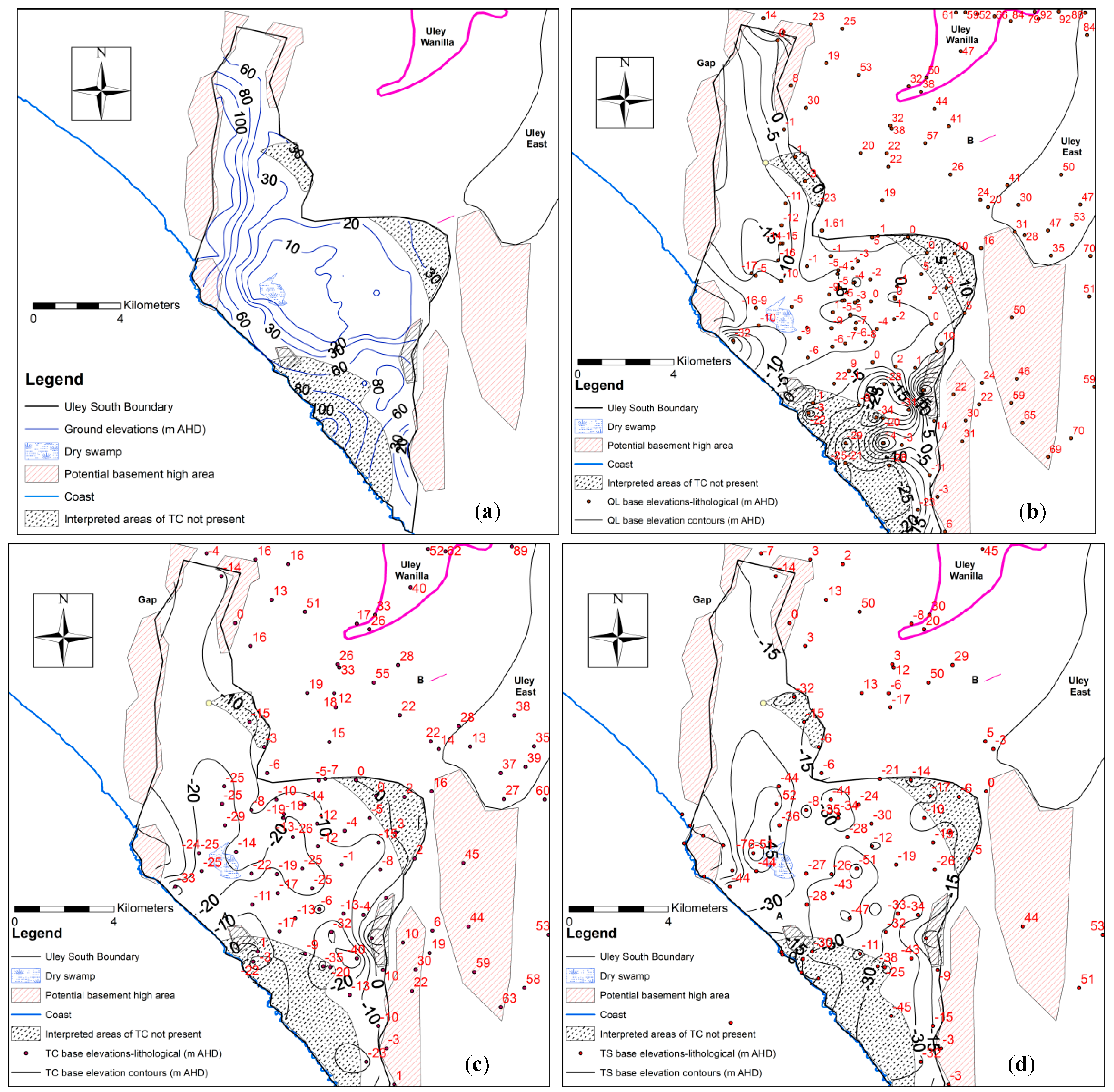
4.1. Uley South Aquifer Elevations: Ground Levels; QL, TC and TS Base Elevations

In north-western part of the Uley South aquifer where much of the area is covered by sand dunes and is inaccessible for drilling, no drillhole data is available. The AEM was used to define base elevations of the QL and TS aquifers and these were correlated with lithology-based layer elevations. A plot of QL-base elevation from lithology versus AEM produced QL-base elevation (Figure 2) was used to assign the layer elevation for the QL aquifer. Overall there is a good agreement between the two data sets, in part because the bore logs were used to constrain the AEM interpretation.
However, the inferred QL base elevations derived from the AEM in areas where limited bore coverage requires a degree of caution. It was difficult to distinguish the base of the TC and TS from the weathered basement [19], as both of these exhibit similar properties, and hence base elevation data was combined with the weathered regolith layer [19]. As it is, AEM produced base elevation data for TC and TS were not overly accurate.
Figure 3 show ground elevations (3a), QL (3b), TC (3c), and TS (3d) base elevations. Ground elevations were derived primarily from surveyed monitoring well elevations supplemented with SRTM [26] elevations in areas where drillholes are not available or very limited.

4.2. Uley South Link to Northern Lenses-QL and TSA aquifers

Since the basins were investigated in the 1960s, the QL in the area between Uley Wanilla and Uley East to the Uley South boundary has been considered a dry area, based on borehole information. The correct hydrogeological practice to identify whether a particular Formation is dry or wet, is to check where the water strike is with respect to the base elevation of the Formation. The watertable is a surface that represents the top of the zone of saturation, which is the area where all available pore spaces are full of groundwater. Once a bore is drilled and completed, water levels may rise and appear even in dry Formations. For this reason, the water strike and not water level elevations are used for determining dry or wet condition of the Formation. Current and historical monitoring well locations are given in Figure 4.
In this study, QL dry area was re-assessed using depths to first-water-strike and depth to QL base. The locations of QL dry bores are shown in Figure 5. Apart from those bores found at the edge of the basin boundary, the depth to first water strike are below the QL base, indicating the presence of dry limestone. The only exceptions are ULE166 and ULE167 (Figure 4a), that are located in the Uley East lens. One interesting feature is that wells located in southern Uley East, ULE173 (TC and basement), ULE166, and ULE167 have not intercepted the TS aquifer; but the basement rock below the TC layer is intercepted. This implies that the Uley South basin is not connected to Uley East lens either through QL (due to dry limestone) or TS aquifers (due to TS not present). This important finding means that south of ULE089, there is no-flow boundary for both QL and TS aquifers.

4.3. Uley South Link to Coffin Bay

Combined lithology and AEM survey produced basement elevations that were contoured to produce a QL base elevation map (Figure 3b). The point measurements presented in Figure 3b were obtained from boreholes that penetrate the QL layer. From the AEM produced QL elevations, a previously unknown basement low area in QL aquifer was identified next to the Coffin Bay—Uley South boundary at the north-western edge of the basin (Gap in Figure 1a) [19]. The basement low area is an indication of potential link to the adjacent Coffin Bay lens. The wells located adjacent to the Uley South north-eastern boundary (Figure 4a,b), LKW029, LKW010, LKW013, and LKW028, were dry wells at the time of drilling, indicating a dry QL layer. Only saturated QL was present in LKW009 and LKW011. Groundwater elevation at LKW011 is about 1.5 m lower than the LKW009 water level and therefore, it is possible that groundwater flow from northern area of the basin could flow into Coffin Bay as well as Uley South coast in the south.

4.4. Uley South Landward Boundary and Inter-Aquifer Leakage

Studies by Harrington et al. [21] and; Somaratne and Frizenschaf [25] show that there is a hydraulic connection of the Uley South unconfined QL aquifer and the Uley Wanilla and Big Swamp areas through the TS aquifer. An important surface feature in the area is the Big Swamp (Figure 1a); with an underlying TC layer making the primary mechanism of discharge through evaporation. In wetter years, Big Swamp overflows and infiltrates into the QL aquifer and leaks into the TS aquifer raising salinity up to 5200 mg·L−1 near Big Swamp [25]. As the brackish water plume moves down gradient along its main flow path, the western edge of the Uley East basin, it has diluted from 5200 mg·L−1 to 960 mg·L−1. The area where aquitard is absent in Uley South landward boundary, the TS aquifer water discharge into the QL aquifer (Figure 1c) results in higher salinity water in the QL [25].
The area of inter-aquifer leakage can be identified from the TEM sections LO1 and LO2. The interpretation of TEM lines are described in previous work of Somaratne and Mann [15] and Somaratne [16] with the following limitations. The variation in resistivity of particular minerals can be enormous, for example limestone: 50–107 Ωm; Marls 3–70 Ωm; Clays: 1–100 Ωm [28]. Other factors such as dissolved minerals in groundwater, fracture zone filled with air or water, and consolidation of geologic materials influence the local changes to resistivity. In most cases, a small change in the percentage of water affects the resistivity [28]. The variation in resistivity of particular minerals can be enormous, for example, limestone: 50–107 Ωm; marls 3–70 Ωm; clays: 1–100 Ωm [28].
The resistivity of fresh water is about 10–100 Ωm [29], overlapping of resistivity values in the saturated zone requires known features for interpretation of TEM sections. In the shallow substructures, presence of water controls much of the resistivity variations. The relationship between the measured resistivity of a geology unit and the resistivity and quantity of contained water has been long established by Archie [30] and others and shows that resistivity in general, is a measure of water saturation and connectivity of pore spaces [31]. Therefore, increasing the number of fractures or porosity tends to decrease the resistivity [31].
The survey was conducted in May 2017 with the onset of winter (June–August) rainfall, and end of the winter in September–October 2017. The rain was intermittent and hence the most active flow paths, such as; epikarst at and near the ground surface, and sinkholes, received some local surface runoff. Figure 6 shows the inverted resistivity sections for survey lines LO1A and LO1B. Resistivity contrast areas were categorized in to four distinct zones. The upper low resistivity zones of up to 5–8 m depth represent the surface and near surface epikarst zone, which temporary hold water in storage, and either directly infiltrated to the watertable via fissures or was lost to the atmosphere through evaporation. Lower resistivity zones at sinkhole locations are the major recharge points either through sinkholes or from surrounding area. This observation is similar to that observed by Jardani et al. [18] in their study on preferential infiltration pathways through sinkholes. Some of the sinkholes may be filled with debris and silt and some may be buried sinkholes as this is a common feature in the basin. Above the watertable in the QL aquifer, a higher resistivity zone may represent the areas of diffuse recharge through the unsaturated zone as the dry or partially dry limestone is a poor electrical conductor. Resistivity varies with the degree of cementation within the calcarenite as indicated by relative difference of resistivity; where >600 Ωm may be strongly cemented calcarenite than 400–600 Ωm range. Below the watertable, resistivity is typically low as indicated by zones of <150 Ωm, but higher resistivity is also found at some locations due to the presence of strongly cemented limestone. For example, at ULE126 (Figure 6a), the driller’s log indicated that the interval from 15.9 m AHD to—3.9 m AHD, as “Sandstone, hard bars” which are of low porosity and therefore show higher resistivity, even under the watertable. At the time of drilling in 1976, the water level of the well ULE126 was at 12 m AHD.
Due to the associated high cost, in general, investigations/monitoring wells are drilled far apart in groundwater basins. Aquifer stratigraphy, particularly the base elevations of aquifers are known only at fully penetrating drillhole locations. For the groundwater model setup, layer elevations are assigned to model cells by either interpolating or extrapolating data between drillhole locations (model grids are usually smaller than the distance between drillholes). However, additional data points can be used from TEM sections where base elevations are changed. For example, between ULE125 and ULE124; and ULE124 and ULE089, the QL aquifer is uplifted and detected from the TEM section. This information can be incorporated to refine hydrogeological frame work of the aquifer. Similarly, combining available lithology data, limestone dry area can be confirmed using TEM sections as it is shown in TS well, ULE089 where QL is dry and the well is located outside the basin boundary.
As a result of QL and TS aquifers depth-coincident in the TC absent area, higher salinity water from TS enters to QL aquifer resulting in pronounced salinity stratification [25]. Evidence of this is found in the QL aquifer monitoring well, ULE197, down-gradient to TC absent area (Figure 4a) where salinity of the QL base is the same as TS aquifer monitoring well, ULE109, located at the same site. In contrast, the southern half of the QL aquifer has no link to the Big Swamp area or to the Uley East, through either QL or TS aquifers due to high basement at the Uley South Boundary (Figure 4a). Therefore, QL water in the southern part of the Uley South is primarily derived from direct rainfall recharge within the Uley South. The ULE139 is a QL aquifer monitoring well located in the southern part, having low EC water compared to ULE197, and shows no salinity stratification (Figure 7) [25].
The leakage of TS water into QL forms an important water balance component that is currently unknown to any degree of accuracy. The poor understanding of the landward boundary leakage area is due to limitation of drillhole information. Therefore, the TEM line (LO2) was laid to identify potential reaches of the inter-aquifer leakage as well as other hydraulic factors of the basin such as aquifer elevations and preferential recharge areas along the section. Figure 8 shows the inverted resistivity sections for survey sections from LO2-A to LO2-C.
The resistivity range in LO2 is as in LO1, with saturated upper layer and lower resistivity zones appearing in areas of sinkholes. The lowest resistivity zone (1 to 55 Ωm) may represent the weathered basement/clay zones, including silty sand of TS aquifer as evidenced from ULE141 (LO2-A). In ULE141, the description of lithology showed that from the surface to 4.1 m AHD, the QL (hard medium dense limestone) shows higher resistivity above the water level. From 4.1 to 1.1 m AHD as the TC, (which comprised of clay to sandy clay unit) and show low TEM resistivity reflecting saturated clay property. However, according to the lithological description (Quartz sand/gravel) of TS occurs in small sections from 1.1 to −4.4 m AHD that is not particularly identifiable from TEM resistivity. Below this, TEM resistivity increases as the weathered basement contains abundant of mica (Figure 9).
It is therefore apparent that minor variations in lithology are not represented, particularly at deeper parts of the section where the resistivity contrast of saturated Formation is not dominant, in this case, saturated TC and TS. An interesting feature in LO2-A is, from 1300 to 1750 m, where TC is absent and recharge through sinkholes may directly recharge both QL and TS aquifers.
Along the LO2-B section, the watertable is 3 to 5 m above the QL base. However, preferential recharge through sinkholes occurs from 4875 to 5375 m in an area where basement is uplifted. As TC is absent from 5125 m to 5375 m, the TS aquifer may get direct vertical recharge. The low resistivity values in unsaturated zone indicate the presence of more open limestone that has high recharge potentials. In contrast, from 7325 to 10,075 m along LO2-C, the resistivity values are high (>400 Ωm), indicating dryness or presence of cemented limestone. TS aquifer monitoring wells ULE127 and ULE092 indicate there is no TC presence at these locations.
TEM sections LO2-D and LO2-E (Figure 10a,b) display similar low recharge potential characteristics as high resistivity is an indication of presence of dry/cemented limestone. From the ULE092 well (LO2-D) to the LKW012 well (LO2-E), TC is absent. An important feature of LO2 (LO2-A, LO2-B, LO2-D, LO2-E where TC is absent) is that TS water flowing from the north-east direction could flow into QL aquifer as an inter-aquifer leakage. This new knowledge is an improvement to previous understanding of the conceptual model.

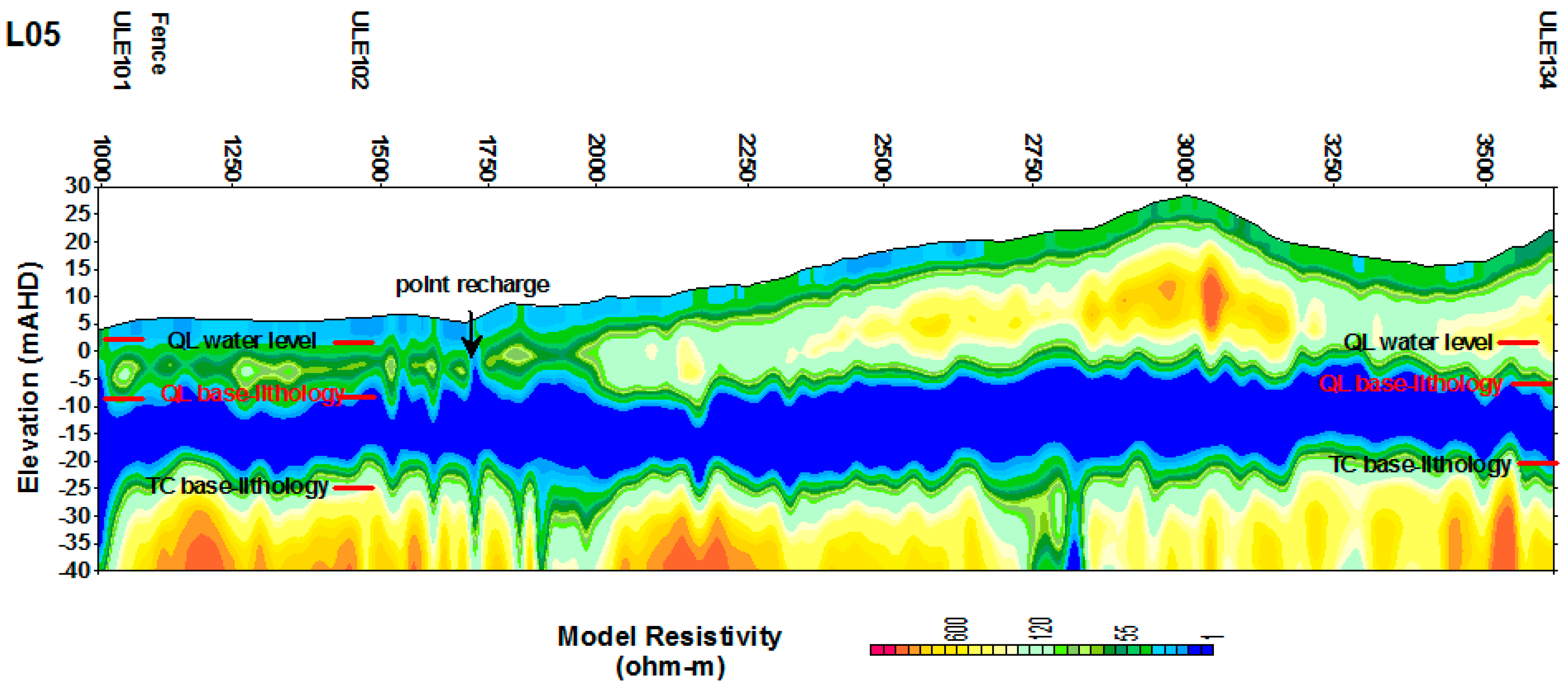
4.5. Recharge and Evidence of Conduit Flow in the Central Basin

Resistivity sections of TEM lines 3 (LO3-A and LO3-B) are given in Figure 11. The line LO3 begins at ULE185 and runs through the centre of the basin. The watertable is found at about 4–5 m AHD. Throughout the sections, TC is present and thickness varies from 7 m at ULE185 to 18 m at ULE137. Point recharge through sinkholes is evidenced throughout the section. As indicated by low resistivity in unsaturated zone, open limestone is present, indicating the central basin is receiving high diffuse recharge. This is in good conformity with recharge estimates using the watertable fluctuations method. Resistivity contrast is dominant in basement and unsaturated zone of LO3-B from 5500 m to 6250 m and beyond where possibly ‘no recharge’ occurs in this part of the aquifer. At ULE145 well, QL base occur at −0.3 m AHD and shallow QL, with saturated thickness of 4 to 5 m, is found in this area, indicating low storage capacity of the QL. As TC is present throughout the LO3-B section, recharge water from sinkholes may distribute within the QL aquifer.
Resistivity section LO5 (Figure 12) runs downgradient to LO3 and across four sinkholes, and QL aquifer monitoring wells ULE101, ULE102, and ULE134. From lithological information, about 15 m thick TC is present in this area. Both point and diffuse recharge is dominant; and the QL aquifer receives high direct recharge. In this regard, TEM sections are particularly useful in identifying aquifer configurations (aquifers, aquitards, and basement), refining layer elevations, and identifying locations of potential point recharge areas. At active or buried sinkhole locations, near vertical low resistivity portions in the profile may be the possible conduits with high recharge. These sinkholes could probably be filled with sediment and become active during recharge events [15]. However, TEM sections provide no direct evidence of the presence of conduit flow paths in the depth-profiles and therefore, gamma and neutron along with EC profiles were taken from all monitoring wells.
Figure 13 displays gamma, neutron, and EC profiles for ULE101, ULE102, and ULE134 wells. The wells were drilled using cable tool method and therefore there are no records of cavity development from lost circulation during drilling. Gamma logs of wells show uniform vertical counts, with 60 (ULE101), 10 (ULE102), and 30 (ULE134) API (American Petroleum Institute) units indicating the presence of possible clayey limestone. Lithological description in the profile varies between “limestone-soft, limestone and clay, limestone-hard or consolidated limestone”. The neutron readings increased indicating higher porosity zone of the profile, with ULE101 at −2.5, −7.5, and −10 m AHD elevations; ULE102 from 0 to −2.5 m AHD and below −5 m AHD, and ULE134 below 0 m AHD. The higher counts of neutron logs, up to 300 cps (cycles per second) indicate more open limestone and presence of conduit porosities. During drilling, it is noticeable when intersecting a large cavity, but not so noticeable if intersecting a small conduit, unless core samples are collected [24]. As no core samples were collected, it may be difficult to identify conduit porosity zones, particularly small-pipe conduits [24], unless neutron logs are used. This aspect is further elaborated in Section 4.6.

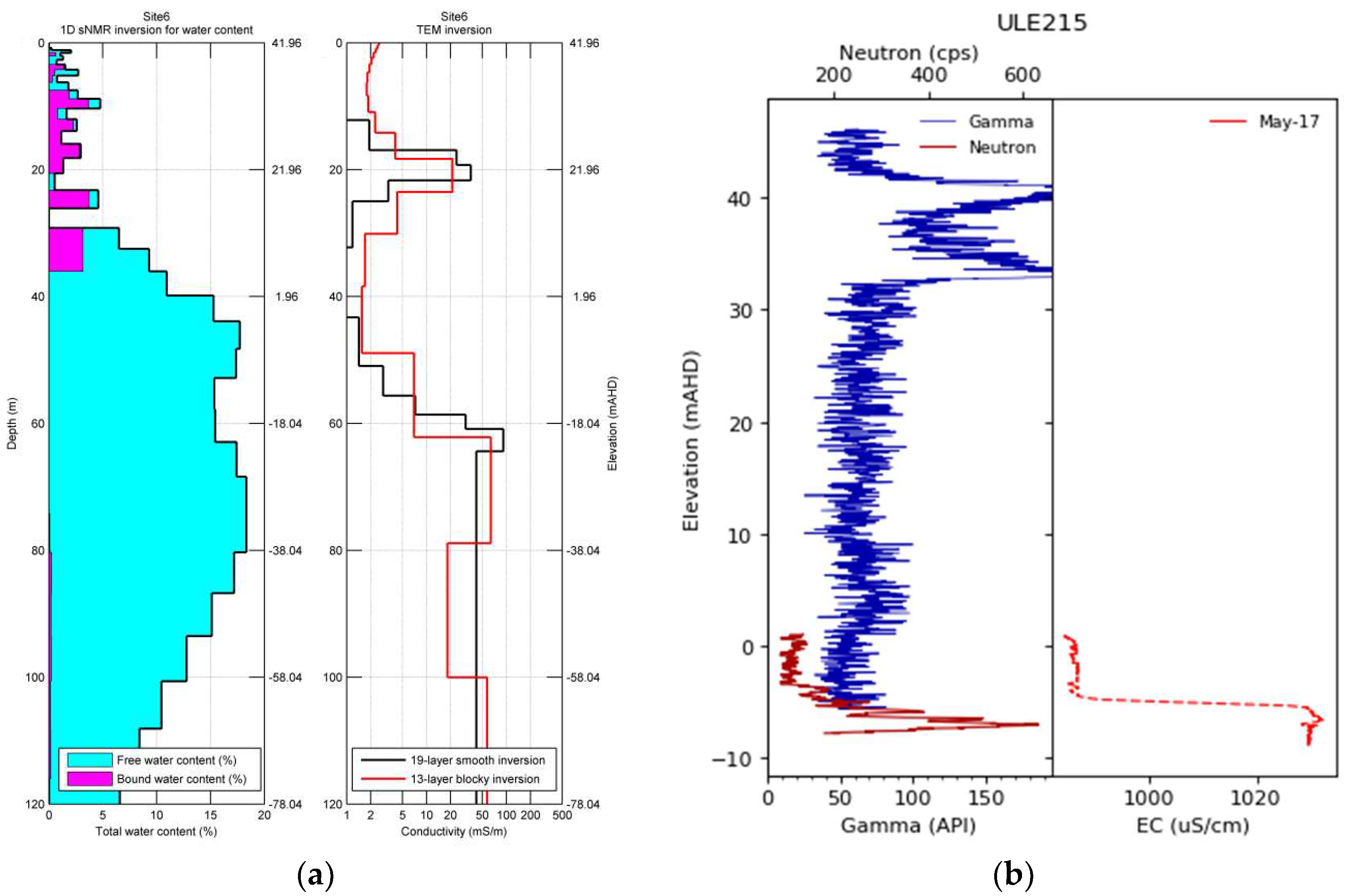
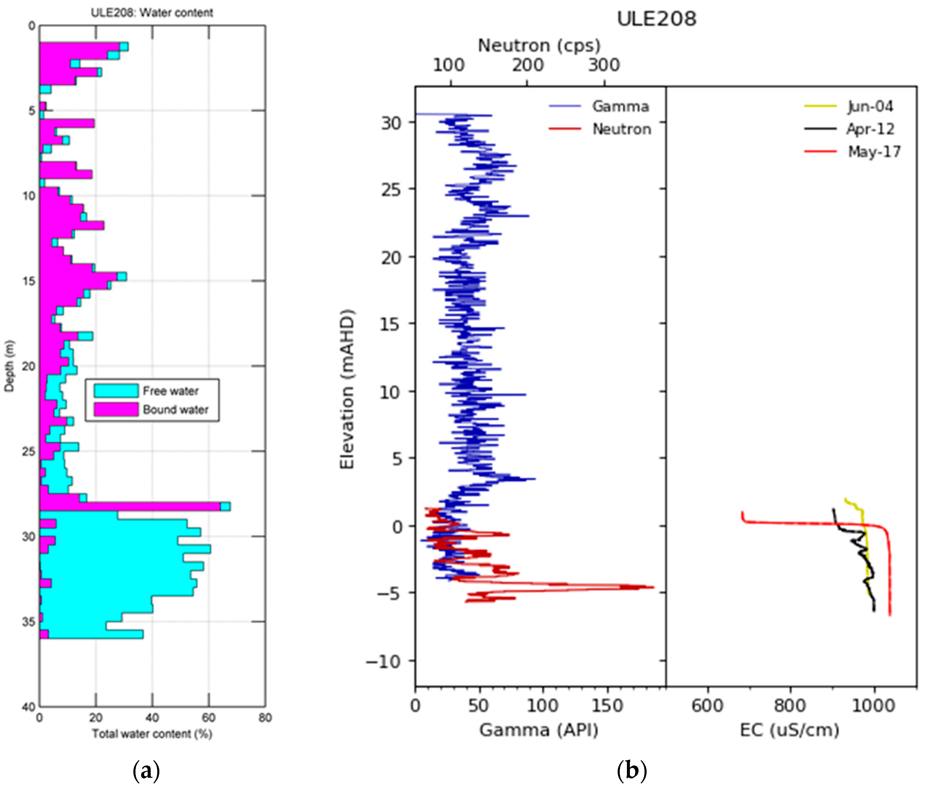
4.6. Nuclear Magnetic Resonance Soundings

Within the Uley South basin, sNMR sounding was carried out at eight sites; and bNMR was carried out at seven selected wells (Figure 5). We provide results for sNMR site 6 where a 250 mm diameter production well (ULE216) and a monitoring well (ULE215) were drilled for testing sNMR findings. At Site 6, a 72.5 m loop was laid for the sNMR sounding [20]. The loop location is about 240 m NW of monitoring well, ULE208, at about 15 m higher ground elevation. The inversion results, displayed in Figure 14 show very little water content (free and bound) in the near surface [20], with a similar pattern continuing to about 25 m depth.
Bound water content increases to about 8% at 30 m depth in this sounding, which matches well with the calcarenite and gravelly layers found at 15 m AHD in the lithology of bore ULE215 located at Site 6. Free water and a very resistive band occur between 30 and 40 m depth, followed by a progressive increase in free water and conductivity below 50 m. At the 53.5 m to 55 m (from −7.8 to −10 m AHD) depth interval, ‘circulation was lost’ during rotary drilling indicating the presence of a cavity. The drilling was terminated at a depth of 60 m (−14.25 m AHD). The presence of a cavity is later confirmed by neutron log obtained in 2017 (Figure 14b). The ULE208 well (Figure 15) was drilled in 2003. At 24−42 m (6.5 m AHD to −11.5 m AHD) depth interval, “lost circulation, no returns, no samples, hard bar at 38 m” was reported in the drillers log and lithological descriptions [16].
Depth to water of ULE208 is about 28 m and drilling logs show ‘lost circulation’ begins in the unsaturated zone indicating the presence of conduit porosity in both saturated and unsaturated zones [23]. The presence of free water up to 60% in ULE208 (Figure 15a) and the deflection of neutron log from 100 to 550 cps (Figure 15b) is an indication of the presence of large cavities, as suggested by lithological description of ‘lost circulation zone’. The occurrence of conduit porosity at about the same elevation in the ULE215 well and ULE208 is an indication of possible inter-linking of conduit porosity in both unsaturated and saturated zones [23]. The lithological description of the ULE215 well shows the occurrence of calcarenite with varying degrees of cementation. The pumping test conducted at the production well near ULE215 at 30 L·s−1 for 600 min produced only 0.061 m drawdown at the test well and no measurable drawdown in a nearby monitoring well (ULE215). This indicates the presence of conduit flows in aquifers and can be detected by sNMR, bNMR, and downhole geophysical logging. In groundwater model setup, Saller et al. [32] discuss the benefits of coupling conduit flow with matrix flow in modelling, but cautioned that uncertainty in locating conduits make it extremely difficult in model calibration. Scanlon et al. [33] applied both lump parameter and distributed parameter models to karst aquifers and showed the ability of using the equivalent porous media model to simulate regional groundwater flow in karstic settings. Nevertheless, even for the application of the equivalent porous media concept, boundaries of higher conductivity zones in the aquifer can be demarcated based on sNMR, bNMR, and downhole geophysics.

5. Conclusions

The use of sNMR, bNMR, TEM, and downhole geophysical surveys have given new insight to the conceptualization of hydrogeological framework of the Uley South Basin. These methods are relatively low cost compared to traditional well drilling; and sNMR and TEM can be applied at sites inaccessible for drilling. Whilst AEM surveys are typically expensive, if data is available, it can be used to inform on layer elevations and conductivities. The use of TEM survey for developing the conceptual model has provided an advantage over relying on drillhole information alone. These include; setting layer elevations where drillhole information are not available; identifying potential reaches of inter-aquifer leakage, and setting the northern boundary condition more accurately; based on resistivity values, identifying areas of diffuse recharge (high resistivity) and the presence of more open limestone or preferential flow paths (low resistivity) zones during recharge period. The use of gamma and neutron logs provides additional information on the presence of conduit porosity zones in the profile that were not detectable with well drilling.
Both sNMR and bNMR techniques are useful for the detection of water and obtaining aquifer porosity and conductivity. This is an important use of geophysical methods for developing conceptual models as obtaining parameters by pump tests are expensive, and yet these parameters are extremely important for numerical model calibration. From bNMR, aquifer saturated hydraulic conductivity is estimated to be in the range of 1–800 m·d−1. The mobile water porosity (which is drainable porosity) can be approximated to a specific yield of the aquifer and is estimated to be in the range of 0.1–0.3 from sNMR; and 0.25 to 0.6 from bNMR. Thus both sNMR and bNMR produced comparable results to pump tested parameters. However, the values of free and bound water content differ in the bNMR and sNMR logs by factors of about 3–4 at each site. This is because bNMR log measures water content within a cylinder 300 mm in diameter, 500 mm in length, and about 2 mm thick [20]. It is possible that at times the volume of investigation from the borehole NMR field partially overlaps the invasion zone caused by drilling [20], leading to over estimation of the porosity. In contrast, sNMR soundings operate with loops on the order of 100 m per side [20] and hence porosity measure is an average over the loop area, leading to an under estimate. In the context of groundwater modelling, upper and lower bounds for aquifer porosity (total water content) and specific yield (mobile water content) can be set up from bNMR and sNMR as initial values for areas where pump tested data is not available. TEM sections are particularly useful in identifying aquifer configurations (aquifers, aquitards, and basement), refining layer elevations, and identifying locations of potential point recharge areas as indicated by low resistivity in unsaturated zone and recharge pathways.

Author Contributions

N.S. conceived the project, provided data interpretation, and written the first draft of the manuscript. G.A. and M.I. added additional interpretation and S.M. executed the TEM survey and analyzed the data. All authors contributed to revision of the article.

Funding

AEM survey was jointly funded by South Australian Water Corporation, Department of Water Land and Biodiversity Conservation and EP Natural Resource Management Board.

Acknowledgments

This study was funded by the South Australian Water Corporation under resource assessment and water security planning in Southern Eyre Peninsula. The helpful comments of three anonymous reviewers are gratefully acknowledged.

Conflicts of Interest

The authors declare no conflict of interest.

References

  1. Yao, Y.; Zheng, C.; Liu, J.; Cao, G.; Xiao, H.; Li, H.; Li, W. Conceptual and numerical models for groundwater flow in an arid inland river basin. Hydrol. Process. 2015, 29, 1480–1492. [Google Scholar] [CrossRef]
  2. Middlemis, H. Groundwater Flow Modelling Guideline; Murray-Darling Basin Commission: Canberra, Australia, 2000.
  3. Rojas, R.; Feyen, L.; Dassargues, A. Conceptual model uncertainty in groundwater modelling: Combining generalized likelihood uncertainty estimation and Bayesian model averaging. Water Resour. Res. 2008, 44. [Google Scholar] [CrossRef]
  4. Neuman, S.; Wierenga, P. A Comprehensive Strategy of Hydrogeologic Modelling and Uncertainty Analysis for Nuclear Facilities and Sites; Rep. NUREG/CR-6805; US Nuclear Regulatory Commission: Washington, DC, USA, 2003.
  5. Refsgaard, J.; van der Sluijs, J.; Brown, J.; van de Keur, P. A framework for dealing with uncertainty due to model structure error. Adv. Water Resour. 2006, 29, 1586–1597. [Google Scholar] [CrossRef] [Green Version]
  6. Ye, M.; Pohlmann, K.F.; Chapman, J.B.; Pholl, G.M.; Reeves, D.M. A model-averaging method for assessing groundwater conceptual model uncertainty. Groundwater 2010, 48, 716–728. [Google Scholar] [CrossRef] [PubMed]
  7. Gillespie, J.; Nelson, S.T.; Mayo, A.L.; Tingey, D.G. Why conceptual groundwater flow models matter: A transboundary example from the Great basin, western USA. Hydrogeol. J. 2012, 20, 1133–1147. [Google Scholar] [CrossRef]
  8. Bakalowicz, M. Chapter 12: Management of karst groundwater resources. In Karst Management; Springer: Berlin, Germany, 2011; pp. S262–S282. [Google Scholar]
  9. Edwards, A.E.; Amatiya, D.M.; Williams, T.M.; Hitchcock, D.R.; James, A.L. Flow characterization in the Santee Cave System in the Chapel Branch Creek watershed, upper coastal plain of South Carolina, USA. J. Cave Karst Stud. 2013, 75, 136–145. [Google Scholar] [CrossRef]
  10. Zhu, J.; Current, J.C.; Dinger, J.S. Challenges of using electrical resistivity method to locate karst conduits—A field case in the Inner Bluegrass Region, Kentucky. J. Appl. Geophys. 2011, 75, 523–530. [Google Scholar] [CrossRef]
  11. Farooq, M.; Park, S.; Song, Y.S.; Kim, J.H.; Tariq, M.; Abraham, A.A. Subsurface cavity detection in a karst environment using electrical resistivity: A case study from Yongweol-ri, South Korea. Earth Sci. Res. J. 2012, 16, 75–82. [Google Scholar]
  12. Ahmed, S.; Carpenter, P.J. Geophysical response of filled sinkholes, soil pipes and associated bedrock fractures in thin mantled karst, east central Illinois. Environ. Geol. 2003, 44, 705–716. [Google Scholar] [CrossRef]
  13. Van Schoor, M. Detection of sinkholes using 2D electrical resistivity imaging. J. Appl. Geophys. 2002, 50, 393–399. [Google Scholar] [CrossRef] [Green Version]
  14. Zhou, W.; Beck, B.F.; Adams, A.L. Effective electrode array in mapping karst hazards in electrical resistivity tomography. Environ. Geol. 2002, 42, 922–928. [Google Scholar] [CrossRef]
  15. Somaratne, N.; Mann, S. Integrated use of geological, geophysical, radiocarbon and stable isotopes data for tracing the conduit flow paths in a small karstic aquifer: Poocher Swamp freshwater lens, South Australia. Environ. Nat. Resour. Res. 2016, 6, 119. [Google Scholar] [CrossRef]
  16. Somaratne, N. Karst conduit networks, connectivity and recharge dynamics of a sinkhole. Environ. Nat. Resour. Res. 2017, 7, 70. [Google Scholar] [CrossRef]
  17. Wedekind, J.E.; Osten, M.A.; Kitt, E.; Herridge, B. Combining surface and downhole geophysical methods to identify karst conditions in North-central Iowa. In Sinkholes and the Engineering and Environmental Impacts of Karst; American Society of Civil Engineers: Reston, VA, USA, 2005; Volume 144, pp. 616–625. [Google Scholar]
  18. Jardani, A.; Revil, A.; Santos, F.; Fauchard, C.; Dupont, J.P. Detection of preferential infiltration pathways in sinkholes using joint inversion of self-potential and EM-34 conductivity data. Geophys. Prospect. 2007, 55, 1–12. [Google Scholar] [CrossRef]
  19. Fitzpatrick, A.; Cahill, K.; Munday, T.; Beren, V. Informing the Hydrogeology of Coffin Bay, South Australia, through the Constrained Inversion of TEMPEST AEM Data; CSIRO: Water for a Healthy Country National Research Flagship; CSIRO Report No. P2009/300; CSIRO: Canberra, Australia, 2009. [Google Scholar]
  20. Davis, A.; Cahill, K.; Hatch, M.; Munday, T. Aquifer Characterization in the Uley South Basin, South Australia, Using NMR: Final Report; CSIRO: Water for a Healthy Country National Research Flagship; Technical Report (EP-31-01-12-14); CSIRO: Canberra, Australia, 2011. [Google Scholar]
  21. Harrington, N.; Zulfic, D.; Wohling, D. Uley Basin Groundwater Modelling Project. Volume 1: Project Overview and Conceptual Model Development; DWLBC Report 2006/01; Government of South Australia: Sydney, Australia, 2006.
  22. Evans, S.L. Estimating Long-Term Recharge to Thin, Unconfined Carbonate Aquifers Using Conventional and Environmental Isotopes Techniques: Eyre Peninsula, South Australia. Master’s Thesis, Flinders University of South Australia, Adelaide, Australia, 1997, unpublished. [Google Scholar]
  23. Somaratne, N. Characteristics of point recharge. Water 2014, 6, 2782–2807. [Google Scholar] [CrossRef]
  24. Somaratne, N. Karst Aquifer Recharge: A case history of over simplification from the Uley South basin, South Australia. Water 2015, 7, 464–479. [Google Scholar] [CrossRef]
  25. Somaratne, N.; Frizenschaf, J. Geological control upon groundwater flow and major ion chemistry with influence on basin management in a coastal aquifer, South Australia. J. Water Resour. Prot. 2013, 5, 1170–1177. [Google Scholar] [CrossRef]
  26. U.S. Geological Survey. Shuttle Radar Topography Mission (SRTM). Available online: https://lta.cr.usgs.gov/srtm (accessed on 21 June 2018).
  27. Wonik, T. Borehole logging. In Environmental Geology: Handbook of Field Methods and Case Studies; Knodel, K., Lange, G., Voigt, H.J., Eds.; Springer Press: Berlin, Germany, 2007; pp. 431–474. [Google Scholar]
  28. Telford, W.M.; Geldart, L.P.; Sheriff, R.E. Applied Geophysics, 2nd ed.; Cambridge University Press: Cambridge, UK, 1990. [Google Scholar]
  29. Palacky, G.V. Resistivity characteristics of geologic targets. In Electromagnetics Methods in Applied Geophysics; Nabighian, M.N., Ed.; Society of Exploration Geophysicists: Tulsa, OK, USA, 1987; Volume 1, pp. 53–129. [Google Scholar]
  30. Archie, G.E. The electrical resistivity log as an aid in determining some reservoir characteristics. Trans. AIME 1942, 146, 54–64. [Google Scholar] [CrossRef]
  31. Cardimona, S. Electrical Resistivity Techniques for Subsurface Investigation; Department of Geology and Geophysics, University of Missouri-Rolla: Rolla, MO, USA, 2002; Available online: https://www.researchgate.net/publication/242692638_ELECTRICAL_RESISTIVITY_TECHNIQUES_FOR_SUBSURFACE_INVESTIGATION (accessed on 21 April 2016).
  32. Saller, S.P.; Ronayne, M.J.; Long, A.J. Comparison of a karst groundwater model with and without discrete conduit flow. Hydrogeol. J. 2013, 21, 1555–1566. [Google Scholar] [CrossRef]
  33. Scanlon, B.R.; Mace, R.E.; Barret, M.E.; Smith, B. Can we simulate regional groundwater flow in a karst system using equivalent porous media models? Case study, baron Springs Edwards Aquifer, U.S.A. J. Hydrol. 2003, 276, 137–158. [Google Scholar] [CrossRef]
Figure 1. (a) Uley South basin with Coffin Bay Lens A, Uley Wanilla, Uley East, and Lincoln Basins; (b) Groundwater elevation contours; (c) Cross section AB [24,25].
Geosciences 08 00226 g001
Figure 2. QL base elevations—Lithology vs. AEM.
Geosciences 08 00226 g002
Figure 3. (a) Ground elevation contours; (b) QL base elevations; (c) TC base elevations; (d) TS base elevations.
Geosciences 08 00226 g003
Figure 4. Monitoring wells; (a) Current; (b) Historic.
Geosciences 08 00226 g004
Figure 5. Dry northern QL bores and TEM lines LO1–LO7.
Geosciences 08 00226 g005
Figure 6. TEM sections for LO1 (a) LO1-A (from ULE126 to ULE124) (b) LO1-B (from ULE124 to ULE089).
Geosciences 08 00226 g006
Figure 7. Gamma, Neutron, and EC profiles for (a) ULE197 (QL), (b) ULE109 (TS), and (c) ULE139 (QL) monitoring wells. The solid line indicates the EC of the production zone.
Geosciences 08 00226 g007
Figure 8. TEM sections for LO2; (a) LO2-A (from ULE141 to ULE121); (b) LO2-B (from ULE121 to ULE127); (c) LO2-C (from ULE127 to ULE092).
Geosciences 08 00226 g008
Figure 9. Resistivity profile at ULE141 site (station 1000 on LO2-A) with lithology.
Geosciences 08 00226 g009
Figure 10. TEM sections for LO2; (a) LO2-D (from ULE092 to LKW034); (b) LO2-E (from LKW034 to LKW012).
Geosciences 08 00226 g010aGeosciences 08 00226 g010b
Figure 11. TEM sections for LO3; (a) LO3-A; (b) LO3-B.
Geosciences 08 00226 g011aGeosciences 08 00226 g011b
Figure 12. TEM section LO5.
Geosciences 08 00226 g012
Figure 13. Gamma, neutron, and EC profiles for (a) ULE101, (b) ULE102, and (c) ULE134.
Geosciences 08 00226 g013
Figure 14. (a) sNMR total water content and conductivity profile at Site 6 [20]; (b) Gamma, neutron, and EC profiles for ULE 215 (surveyed ground elevation 45.7 m AHD. There is a discrepancy in SRTM [26] based elevation used at Site 6 compared to the surveyed elevations).
Geosciences 08 00226 g014
Figure 15. (a) sNMR total water content and conductivity profile at ULE208 [20]; (b) Gamma, neutron, and EC profiles for ULE 208 (surveyed ground elevation 30.5 m AHD).
Geosciences 08 00226 g015

